Charmonium Theory

Aida X. El-Khadra

Physics Department, Ohio State University, 174 W 18th Ave, Columbus, OH 43210, U.S.A.

Abstract. Recent theoretical progress in calculations of the spectrum and decays of charmonium is reviewed. Traditionally, our understanding of charmonium was based on potential models. This is now being replaced by first principles.

INTRODUCTION

The charmonium system is at present among the theoretically best understood hadronic systems. The charm quark mass is large compared to the typical QCD scale, $\Lambda_{QCD}$. The $c\bar{c}$ bound states are therefore governed by non-relativistic dynamics. Historically, while the QCD potential was not known from first principles, relatively simple guesses for phenomenological potentials had proven quite successful in describing the experimentally measured bound state spectrum of charmonium [1]. Likewise, for annihilation decays of charmonium, an intuitive factorization ansatz, involving the wave function at the origin (calculable in potential models) worked quite well, for the most part.

This model-based theoretical understanding is now being replaced by first principles. For charmonium spectroscopy, the progress comes from using lattice QCD. Charmonium decays can be treated rigorously with the help of non-relativistic QCD (or NRQCD).

Lattice field theory offers a systematic first principles approach to solving QCD. It has been argued by Lepage [2] that charmonium is one of the easiest systems to study with lattice QCD, with the potential of complete control over all systematic errors. Finite-volume errors are much easier to control for quarkonia than for light hadrons. Lattice-spacing errors, on the other hand, can be larger for quarkonia and need to be considered. An alternative to reducing the lattice spacing in order to control this systematic error is improving the action (and operators). For quarkonia, the size of lattice-spacing errors in a numerical simulation can be anticipated by calculating expectation values of the corresponding operators using potential model wave functions. They are therefore ideal systems to test and establish improvement techniques. Most of the work of phenomenological relevance is done in what is generally referred to as the “quenched” (and sometimes as the “valence”) approximation. In this approximation gluons are not allowed to split into quark - anti-quark pairs (sea quarks). In the case of charmonium, potential model phenomenology can be used to estimate this systematic error. Control over systematic errors in turn allows the extraction of Standard Model parameters from the quarkonia spectra.

Non-relativistic systems, like charmonium, are best described with an effective field theory, non-relativistic QCD (or NRQCD). It was shown in Ref. [3] that the application of NRQCD to the problem of annihilation decays of quarkonium leads to a general factorization formula. It reproduces the earlier (ad hoc) factorization ansatz for S-wave decays while putting it on a firm theoretical footing. In the case of P-wave decays, the previous ansatz is modified.

Lattice QCD and NRQCD are introduced in the following subsections. The remainder of the talk is organized in two parts. The first part reviews recent progress in calculations of the charmonium spectrum based on lattice QCD. The second part reviews progress in understanding charmonium decays based on NRQCD.

An Introduction to Lattice QCD

Lattice Field theory is formulated using the Feynman path integral in Euclidean space. The quantities that are actually calculated are expectation values of Greens functions (${\cal G}$), which are products of gauge and fermion fields. The physical quantities of interest, hadron masses, matrix elements, etc., are then extracted from these Greens functions.

The discretization of space-time (with lattice spacing $a$) regulates the path integral at short distances or in the ultraviolet. A finite volume (of length $L$) is necessary for numerical techniques and also introduces an infrared cut-off or momentum-space discretization. The vacuum expectation of a Greens function, ${\cal G}$, is defined as:

$$\langle{\cal G}\rangle=\lim_{L\rightarrow\infty}\,\lim_{a\rightarrow 0}\,\langle{\cal G}\rangle_{L,a}\;\;,\;\;\;\langle{\cal G}\rangle_{L,a}=Z^{-1}_{L,a}\int{\cal D}\psi{\cal D}\bar{\psi}{\cal D}U\,{\cal G}\,e^{-S_{\rm lat}}\;\;\;.$$ (1)

$Z_{L,a}$ normalizes the expectation value. I have omitted spin and color indices for compactness. The gauge degrees of freedom are written as (path ordered) exponentials of the gauge field, $A_{\mu}$:

$$U_{\mu}(x)=e^{i\int_{x}^{x+a}dx^{\prime}A_{\mu}(x^{\prime})}\simeq e^{iaA_{\mu}(x)}\;\;\;,$$ (2)

which makes it easy to maintain gauge invariance. The link fields, $U$, are $SU(3)$ matrices. The (Euclidean) QCD action,

$$S=S_{g}+S_{f}\;\;,\;\;\;\;S_{g}=\frac{1}{4g^{2}}\int d^{4}x\,F_{\mu\nu}F^{\mu\nu}\;\;,\;\;\;\;S_{f}=\int d^{4}x\,\bar{\psi}(x)(D\!\!\!\!/+m)\psi(x)\;\;.$$ (3)

is discretized, such that Eq. (3) is recovered in the the continuum ($a\rightarrow 0$) limit:

$$S_{\rm lat}=S+{\cal O}(a^{n})\;\;,\;\;\;n\geq 1\;\;\;.$$ (4)

I will not go into the explicit formulations of $S_{\rm lat}$ here, but instead refer the reader to pedagogical introductions [4]. The most common form for the gauge action is Wilson’s [5], written in terms of plaquettes – products of $U$ fields around the smallest closed loop on a lattice. Wilson’s gauge action has discretization errors of ${\cal O}(a^{2})$.

For fermions the situation is more complicated. The discretization of

$$M\equiv D\!\!\!\!/+m\;\;,$$ (5)

is a sparse, finite dimensional matrix. Two different approaches are in use. In Wilson’s formulation [6] chiral symmetry is explicitly broken, but restored in the continuum limit. The pay-off is a solution of the so-called fermion doubling problem. Staggered fermions [7] keep a $U(1)$ chiral symmetry at the expense of dealing with 4 degenerate flavors of fermions.

Eq. (1) emphasizes that QCD is a limit of lattice QCD. However, in numerical calculations these limits cannot be taken explicitly, only by extrapolation. This is feasible, because theoretical guidance for both limits is available. The zero-lattice-spacing limit is guided by asymptotic freedom, since the lattice spacing is related to the gauge coupling by the renormalization group. Quantum field theories in large but finite volumes have also been analyzed theoretically [8].

In a numerical calculation the limits are taken by considering a series of lattices, as illustrated in Figure 1. While keeping the physical volume (or $L$) fixed, the lattice spacing is successively reduced; then, keeping the lattice spacing fixed the volume is increased. The calculation is in the continuum (infinite volume) limit once the hadron spectrum or matrix elements of interest become independent of the lattice spacing (volume).

Figure 1: Illustration of the continuum and infinite-volume limits.

In practice, however, limitations in computational resources do not permit the ideal lattice QCD calculation just described. In particular, the computational cost of reducing the lattice spacing naively scales like $(L/a)^{4}$. (The computational cost is really higher, because of numerical problems at smaller lattice spacings.) Eq. (4) illustrates an alternative. By improving the discretization errors in the lattice action (and operators), the continuum limit can be reached at coarser lattice spacings than before. Simulations with improved actions can come at only a slightly higher computational price. The ideas underlying improvement were developed some time ago [9, 10, 11], and have since been revitalized [12, 13, 14, 15].

If the quark mass is large compared to the typical QCD scale, $\Lambda_{QCD}$, effective theories (such as NRQCD) are most adequate in describing the physics [16]. In that case, the lattice spacing cannot be taken to zero. Lattice-spacing errors can, however, be systematically reduced by improvement [17].

The problem is now (more or less) set up. I again refer the reader to the literature [4] for more details on the organization of typical lattice QCD calculations.

An Introduction to NRQCD (Non-Relativistic QCD)

In non-relativistic systems, the velocity $v$ of the heavy quark inside the bound state is a small parameter; in charmonium $v^{2}\sim 0.3$. The important momentum scales with regard to the structure of the bound state are the heavy quark momentum ($mv$) and its kinetic energy ($mv^{2}$). Momenta of the order of the heavy quark mass ($m$), or above, are relatively unimportant in the bound state dynamics. If $v$ is small enough, then all the different momentum scales are well separated, in particular:

$$\Lambda_{\rm QCD}\;,\;mv^{2}\;,\;mv\ll m$$ (6)

The most adequate description of such systems is in terms of an effective field theory, non-relativistic QCD (or NRQCD). The theory has a cut-off $\Lambda\sim m$. The effective lagrangian can be written as an expansion in powers of $1/m$. The NRQCD lagrangian is [16]

$${\cal L}_{\rm NRQCD}={\cal L}_{\rm light}+{\cal L}_{\rm heavy}+\delta{\cal L}\;\;.$$ (7)

${\cal L}_{\rm light}$ is the fully relativistic lagrangian for the light quarks and gluons. ${\cal L}_{\rm heavy}$ is the heavy quark (and anti-quark) lagrangian,

$${\cal L}_{\rm heavy}=\psi^{\dagger}\left(iD_{0}+\frac{\mbox{\boldmath${D}$}}{2m}\right)\psi+\chi^{\dagger}\left(iD_{0}-\frac{\mbox{\boldmath${D}$}}{2m}\right)\chi\;\;,$$ (8)

where $\psi$ and $\chi$ are 2-component Pauli spinors describing quark and anti-quark degrees of freedom.

Relativistic effects of full QCD introduce corrections to Eq. (8) which appear in $\delta{\cal L}$ as local, non-renormalizable interactions, with coefficients that are calculable in perturbation theory [16, 17]. In principle, infinitely many terms must be considered to reproduce full QCD. In practice, however, only a finite number is needed, since every operator scales with a certain power of $v$, as shown in Ref. [17]. These power counting rules (e.g., $\psi\sim(mv)^{(3/2)}$, $\mbox{\boldmath${D}$}\sim mv$, etc.) effectively order the terms in the NRQCD lagrangian by powers of $v$.

The annihilation of a $Q\bar{Q}$ pair occurs at momenta of order $m$. This short distance physics cannot be treated directly in NRQCD. However, the annihilation contribution to low-energy $Q\bar{Q}\rightarrow Q\bar{Q}$ scattering can be incorporated in NRQCD by adding local 4-fermion operators to $\delta{\cal L}$ [3],

$$\delta{\cal L}_{\rm 4-fermion}=\sum_{i}\frac{f_{i}}{m^{d_{i}-4}}\,{\cal O}_{i}\;\;.$$ (9)

For example,

$${\cal O}_{1}(^{1}S_{0})=\psi^{\dagger}\chi\chi^{\dagger}\psi\;\;.$$ (10)

The $f_{i}$ are again calculable in perturbation theory as expansions in $\alpha_{s}(m)$.

CHARMONIUM SPECTROSCOPY

Two different formulations for fermions have been used in lattice calculations of these spectra. Lepage and collaborators [2, 17] have adapted the NRQCD formalism to the lattice regulator. Several groups have performed numerical calculations of quarkonia in this approach. In Ref. [18] the NRQCD action is used to calculate the charmonium spectrum, including terms of ${\cal O}(mv^{4})$ and ${\cal O}(a^{2})$. In addition, this group has calculated the $b\bar{b}$ spectrum in the quenched approximation ($n_{f}=0$) [19] and also using gauge configurations that include 2 flavors of sea quarks [20, 21].

The Fermilab group [13] developed a generalization of previous approaches, which encompasses the non-relativistic limit for heavy quarks as well as Wilson’s relativistic action for light quarks. Lattice-spacing artifacts are analyzed for quarks with arbitrary mass. Ref. [22] uses this approach to calculate the $c\bar{c}$ (and $b\bar{b}$) spectra in the quenched approximation. We considered the effect of reducing lattice-spacing errors from ${\cal O}(a)$ to ${\cal O}(a^{2})$.

The two groups mentioned above use gauge configurations generated with the Wilson action, leaving ${\cal O}(a^{2})$ lattice-spacing errors in the results. The lattice spacings, in this case, are in the range $a\simeq 0.05-0.2$ fm. Ref. [15] uses an improved gauge action (to ${\cal O}(a^{4})$) together with a non-relativistic quark action improved to the same order (but without spin-dependent terms) on coarse ($a\simeq 0.4-0.24$ fm) lattices.

The first step in any lattice QCD calculation is the determination of the two free free parameters of the theory, the gauge coupling and quark mass, from experiment. This is discussed in the following subsection. The results for the charmonium spectrum from all groups are summarized in Figure 2.

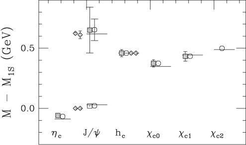
Figure 2: A comparison of lattice QCD results for the $c\bar{c}$ spectrum using the quenched approximation ($n_{f}=0$). The error bars are statistical only. —: Experiment; $\Box$: FNAL [22]; $\circ$: NRQCD [18]; $\Diamond$: ADHLM [15].

The agreement between the experimentally-observed spectrum and lattice QCD calculations is respectable. As indicated in the preceding paragraphs, the lattice artifacts are different for all groups. Figure 2 therefore emphasizes the level of control over systematic errors. I should also note, however, that the theoretical errors (from the Monte Carlo integration alone) are still much larger than the experimental ones. They also grow with every level of excitation considered.

The first quarkonium results with 2 flavors of degenerate sea quarks have appeared [20, 23, 24] with lattice-spacing and finite-volume errors similar to the quenched calculations, significantly reducing this systematic error. In Refs. [23, 24] the 1P-1S splitting in charmonium is calculated, while Ref. [20] considers the $b\bar{b}$ spectrum.

Several systematic effects associated with the inclusion of sea quarks must still be studied. They include the dependence on the quarkonium spectrum of the number of flavors of sea quarks and the sea-quark action (staggered vs. Wilson). The inclusion of sea quarks with realistic light-quark masses is very difficult. However, quarkonia are expected to depend only very mildly on the masses of the light quarks. This systematic error has not been included yet and should be checked numerically.

The first (and second) generation of lattice QCD calculations, as described here, is focused on the simplest physical quantities, like the low lying states or simple (decay) matrix elements, to establish the method. Once first principles calculations have been achieved, this technology can and will (given sufficient motivation) be used to look at more complicated problems, like higher excited states, mixing with glueballs, hybrids, etc.

Standard Model Parameters from Charmonium

The first step, the determination of the lattice gauge coupling and quark mass, follows from comparing appropriate quantities calculated on the lattice with the corresponding experimental measurements. The lattice parameters can then be converted to their counterparts in continuum QCD with perturbation theory.

Precise determinations of Standard Model parameters are an interesting by-product of lattice QCD calculations of charmonium (and bottomonium). However, the theoretical uncertainties must be reduced by an order of magnitude before they become comparable to the present experimental errors. After discussing the determination of the lattice spacing (which sets the scale in Figure 2), I will summarize the results for the strong coupling and the charm quark mass from charmonium.

Determination of the Lattice Spacing, $a$

The input gauge coupling sets the lattice spacing, $a$, which is determined in physical units by comparing a suitable quantity on the lattice with its experimental value. For this purpose, one should identify quantities that are insensitive to lattice errors. In quarkonia, spin-averaged splittings are good candidates. The experimentally observed 1P-1S and 2S-1S splittings depend only mildly on the quark mass (for masses between $m_{b}$ and $m_{c}$), as shown in table 1.

Table 1: Spin-averaged splittings in the $J/\psi$ and $\Upsilon$ systems in comparison.

	$c\bar{c}$ (MeV)	$b\bar{b}$ (MeV)
$m({\rm 1P-1S})$	$456.8$	$452\;\;\;$
$m({\rm 2S-1S})$	$596\;\;\;$	$563\;\;\;$
$m({\rm 2P-1P})$	—	$359.7$

Figure 3 shows the observed mass dependence of the 1P-1S splitting in a lattice QCD calculation. The comparison between results from different lattice actions illustrates that higher-order lattice-spacing errors for these splittings are small[20, 22]. In contrast, Figure 4 shows the hyperfine splitting as an example of a quantity that strongly depends on both the mass and the lattice action. It would therefore be a poor choice for a determination of the lattice spacing.

Figure 3: The 1P-1S splitting as a function of the 1S mass (statistical errors only) from Ref. [22]; $\Box$: ${\cal O}(a^{2})$ errors; $\times$: ${\cal O}(a)$ errors.

Figure 4: The hyperfine splitting as a function of the 1S mass (statistical errors only) from Ref. [22]; $\Box$: ${\cal O}(a^{2})$ errors; $\times$: ${\cal O}(a)$ errors.

The Strong Coupling, $\alpha_{s}$

Within the framework of lattice QCD the conversion from the bare to a renormalized coupling can, in principle, be made non-perturbatively [25]. An alternative is to define a renormalized coupling through short distance lattice quantities [26]. The size of higher-order corrections associated with the above defined coupling constant can be tested by comparing perturbative predictions for short-distance lattice quantities with non-perturbative results [26].

At this point the relation to the $\overline{{\rm MS}}$ coupling is known to 1-loop, leading to a $5\,\%$ uncertainty. It has recently been calculated to 2-loops [27] in the quenched approximation (no sea quarks, $n_{f}=0$). The extension to $n_{f}\neq 0$ will significantly reduce the uncertainty due to the use of perturbation theory.

Sea Quark Effects.  Calculations that properly include all sea-quark effects do not yet exist. If we want to make contact with the “real world”, these effects have to be estimated phenomenologically or extrapolated away.

The phenomenological correction necessary to account for the sea-quark effects omitted in calculations of quarkonia that use the quenched approximation gives rise to the dominant systematic error in these calculations [28, 29]. Similar ideas were used to correct for sea-quark effects in early calculations of quarkonia spectra from the heavy-quark potential calculated in quenched lattice QCD [30].

By demanding that, say, the spin-averaged 1P-1S splitting calculated on the lattice reproduce the experimentally observed one (which sets the lattice spacing, $a^{-1}$, in physical units), the effective coupling of the quenched potential is in effect matched to the coupling of the effective 3 flavor potential at the typical momentum scale of the quarkonium states in question. The difference in the evolution of the zero flavor and 3,4 flavor couplings from the effective low-energy scale to the ultraviolet cut-off, where $\alpha_{s}$ is determined, is the perturbative estimate of the correction.

For comparison with other determinations of $\alpha_{s}$, the $\overline{{\rm MS}}$ coupling can be evolved to the $Z$ mass scale. An average [31] of Refs. [22, 29] yields for $\alpha_{s}$ from calculations in the quenched approximation:

$$\alpha^{(5)}_{\overline{{\rm MS}}}(m_{Z})=0.110\pm 0.006\;\;\;.$$ (11)

The experimental error in this determination from the quarkonium mass splitting is much smaller than the theoretical uncertainty and does not contribute to the total.

The phenomenological correction described in the previous paragraphs has been tested from first principles in Refs. [20, 23, 24]. All groups calculate quarkonium splittings with 0 and 2 flavors of sea quarks. After extrapolating to the physical 3 flavor case and evolving the coupling to $m_{Z}$, Refs. [23, 24] find for the strong coupling from charmonium

$$\alpha^{(5)}_{\overline{{\rm MS}}}(m_{Z})=0.111\pm 0.005$$ (12)

in good agreement with the previous result in Eq. (11). The total error is now dominated by the rather large statistical errors and the perturbative uncertainty.

At present, the result of Ref. [20] has the smallest statistical and systematic errors for the strong coupling (in this case from the $b\bar{b}$ spectrum):

$$\alpha^{(5)}_{\overline{{\rm MS}}}(m_{Z})=0.115\pm 0.002\;\;\;.$$ (13)

Phenomenological corrections are a necessary evil that enter most coupling constant determinations. In contrast, lattice QCD calculations with complete control over systematic errors will yield truly first-principles determinations of $\alpha_{s}$ from the experimentally observed hadron spectrum.

At present, determinations of $\alpha_{s}$ from the experimentally measured quarkonia spectra using lattice QCD are comparable in reliability and accuracy to other determinations based on perturbative QCD from high energy experiments. They are therefore part of the 1994 world average for $\alpha_{s}$ [31]. The phenomenological corrections for the most important sources of systematic errors in lattice QCD calculations of quarkonia are now being replaced by first principles, which will significantly increase the accuracy of $\alpha_{s}$ determinations from quarkonia. In particular, the systematic errors associated with the inclusion of sea quarks into the simulation have to be checked.

The Charm Quark Mass

Because of confinement, the quark masses cannot be measured directly, but have to be inferred from experimental measurements of hadron masses, and depend on the calculational scheme employed. In lattice QCD quark masses are determined non-perturbatively, by tuning the input lattice quark mass ($m^{\rm lat}_{Q}$) so that, for example, the experimentally observed $J/\psi$ mass is reproduced by the calculation.

Phenomenologically useful quark masses are the perturbatively defined pole and $\overline{{\rm MS}}$ masses, which the bare lattice mass can be related to by perturbation theory:

$$m_{Q}^{\rm pole}=Z^{\rm pole}_{m}\,m^{\rm lat}_{Q}\;\;\;,\hskip 56.9055ptm_{Q}^{\overline{{\rm MS}}}(m_{Q})=Z^{\overline{{\rm MS}}}_{m}\,m^{\rm lat}_{Q}\;\;\;.$$ (14)

Of course, as always, all systematic errors arising from the lattice QCD calculation need to be under control for a phenomenologically interesting result; in particular, the systematic error introduced by the (partial) omission of sea quarks has to be removed. The short-distance corrections that introduced the dominant uncertainty to the $\alpha_{s}$ determination from quarkonia are absent for the pole mass determination, because this effective mass does not run for momenta below its mass. An analysis of the $b$-quark mass from the $b\bar{b}$ spectrum with and without sea quarks is consistent with this estimate [21].

Ref. [32] analyzes the the charm quark mass from the charmonium spectrum with the preliminary result, $m_{c}^{\rm pole}=1.5(2)$ GeV.

The $\overline{{\rm MS}}$ mass for the charm quark has also been determined from a compilation of $D$ meson calculations in the quenched approximation [33], with $m_{c}^{\overline{{\rm MS}}}(2\,{\rm GeV})=1.47(28)$ GeV. The error includes statistical errors from the original calculations and the perturbative error. However sea-quark effects cannot, in this case, be estimated phenomenologically, leaving this systematic error uncontrolled.

CHARMONIUM DECAYS

Historically [34, 1], charmonium annihilation decays were treated with a factorization ansatz, which divides the decay rate into a short distance, perturbative part, and a long distance, non-perturbative part, usually parametrized as the wave function at the origin, $R(0)$. This ansatz worked quite well for S-wave decays, even after including radiative corrections at next-to-leading order [35]. For P-wave decays, the long distance piece was identified as the derivative of the wave function at the origin, $R^{\prime}(0)$. However, the radiative corrections were found to have infra-red divergences [36] for $J=1$ P-wave states already at leading order, and for $J=0,2$ P-wave states at next-to-leading order, preventing reliable theoretical predictions. This ansatz also did not allow for a systematic inclusion of higher Fock states, or relativistic corrections.

If the effective field theory framework of NRQCD is used to describe annihilation decays, it was shown [3] that a general factorization formula holds for the decay rates. The annihilation decay rate of a quarkonium state $A$ can be written as

$$\Gamma(A)=2\;{\rm Im}\langle A|\delta{\cal L}_{\rm 4-fermion}|A\rangle\;\;.$$ (15)

Using Eq. (9) this gives

$$\Gamma(A)=\sum_{i}\frac{F_{i}}{m^{d_{i}-4}}\;\langle A|{\cal O}_{i}|A\rangle\;\;\;.$$ (16)

The coefficients $F_{i}$ are the imaginary parts of the $f_{i}$ in Eq. (9). Because of the power counting rules of Ref. [17], the matrix elements scale with some power of the velocity,

$$\langle A|{\cal O}_{i}|A\rangle\sim v^{2n}\;\;,$$ (17)

which usually increases as higher dimensional operators are considered in the sum of Eq. (16). Effectively, this approach expresses the quarkonium decay rates as expansions in the the short distance parameter $\alpha_{s}(m)$ and the long distance parameter $v^{2}$. The desired accuracy of the theoretical prediction thus serves as a truncation criterion for the (infinite) sum in Eq. (16).

The matrix elements in Eq. (16) are calculable from first principles using lattice NRQCD. These calculations are in progress by the ANL group [37]. In the meantime, the matrix elements can also be extracted from experimental measurements of charmonium decay rates.

It was shown in Ref. [3] that heavy-quark spin symmetry and the vacuum-saturation approximation reduces the number of independent matrix elements that have to be determined non-perturbatively or phenomenologically.

The matrix elements of the 4-fermion operators, which contribute to the charmonium decays into light hadrons can be simplified using the vacuum saturation approximation. This approximation is valid in NRQCD up to relative order $v^{4}$. For example,

$$\langle\eta_{c}|\psi^{\dagger}\chi\chi^{\dagger}\psi|\eta_{c}\rangle=|\langle 0|\chi^{\dagger}\psi|\eta_{c}\rangle|^{2}(1+{\cal O}(v^{4}))\;\;.$$ (18)

This relates the matrix elements appearing in electro-magnetic charmonium decays to those in strong decays (into light hadrons).

Heavy-quark spin symmetry relates matrix elements of states in the same radial and orbital levels but different spins. For example,

$$\mbox{\boldmath${\epsilon}$}^{*}\cdot\langle 0|\chi^{\dagger}\mbox{\boldmath${\sigma}$}\psi|J/\psi\rangle=\langle 0|\chi^{\dagger}\psi|\eta_{c}\rangle(1+{\cal O}(v^{2}))\;\;.$$ (19)

The following two subsections discuss the application of this approach to S- and P-wave decays, using specific examples.

S-Wave Decays

I discuss the theoretical knowledge of S-wave decays using $\eta_{c}\rightarrow\gamma\gamma$ as an example. At leading order in $v^{2}$ the rate is

$$\Gamma(\eta_{c}\rightarrow\gamma\gamma)=\frac{F_{\gamma\gamma}(^{1}S_{0})}{m^{2}}|\overline{R_{S}}|^{2}\;\;,$$ (20)

where by spin symmetry (see Eq. (19)) $\overline{R_{S}}$ can be taken as $\overline{R_{\eta_{c}}}$ or the spin-averaged combination of $\overline{R_{\eta_{c}}}$ and $\overline{R_{\psi}}$, with

$$\overline{R_{\eta_{c}}}=\sqrt{\frac{2\pi}{3}}\;\langle 0|\chi^{\dagger}\psi|\eta_{c}\rangle\;\;.$$ (21)

The other $\eta_{c}$ and $J/\psi$ decays differ from Eq. (20) in the short distance coefficient but, using Eqs. (18) and (19), have the same long distance parameter, $\overline{R_{S}}$. Identifying $\overline{R_{S}}$ with the wave function at the origin, $R_{S}(0)$, leads back to the old factorization ansatz. The short distance coefficients, $F_{i}$, are known to next-to-leading order in $\alpha_{s}$.

At next to leading order in $v^{2}$, the decay rate becomes

$$\Gamma(\eta_{c}\rightarrow\gamma\gamma)=\frac{F_{\gamma\gamma}(^{1}S_{0})}{m^{2}}\;|\overline{R_{\eta_{c}}}|^{2}+\frac{G_{\gamma\gamma}(^{1}S_{0})}{m^{4}}\;{\rm Re}(\overline{R_{S}}^{*}\overline{\mbox{\boldmath${\nabla}$}^{2}R_{S}})\;\;.$$ (22)

Now the difference between $\overline{R_{\eta_{c}}}$ and $\overline{R_{S}}$, which is of order $v^{2}$ (see Eq. (19)) has to be taken into account for consistency. $\overline{\mbox{\boldmath${\nabla}$}^{2}R_{S}}$ can be interpreted as the laplacian of the wave function at the origin,

$$\langle 0|\chi^{\dagger}(\mbox{\boldmath${D}$}^{2})\psi|\eta_{c}\rangle=\sqrt{\frac{3}{2\pi}}\;\overline{\mbox{\boldmath${\nabla}$}^{2}R_{S}}\;(1+{\cal O}(v^{2}))\;\;.$$ (23)

The short distance coefficients, $G_{i}$, are known to leading order in $\alpha_{s}$.

The long distance parameters, $\overline{R_{\eta_{c}}}$, $\overline{R_{\psi}}$ and $\overline{\mbox{\boldmath${\nabla}$}^{2}R_{S}}$ can be calculated in lattice NRQCD, estimated using potential models or extracted from a phenomenological analysis of experimental data. The relative errors (from the truncation of the perturbative and non-relativistic series) are $\alpha_{s}(m_{c})^{2}$, $\alpha_{s}(m_{c})v^{2}$ and $v^{4}$, adding up to ${\raise 1.29167pt\hbox{$<$\kern-7.5pt\lower 4.30554pt\hbox{$\sim$}}}15\;\%$.

It is not inconceivable that at least for the electro-magnetic S-wave decays some (or all) of the higher order calculations will be performed, reducing the theoretical error accordingly.

P-Wave Decays

The structure of P-wave decay rates is more complicated than that of S-waves. I shall start with a simple example first, the decay $\chi_{cJ}\rightarrow\gamma\gamma$.

$$\Gamma(\chi_{cJ}\rightarrow\gamma\gamma)=\frac{F_{\gamma\gamma}(^{3}P_{J})}{m^{4}}\;|\overline{R^{\prime}_{P}}|^{2}\;\;,$$ (24)

where again, by spin symmetry $\overline{R^{\prime}_{P}}$ can be taken from the matrix elements of any of the P-wave states (or their spin-averaged combination). For example,

$$\langle 0|\chi^{\dagger}(\frac{1}{2}\mbox{\boldmath${D\cdot\sigma}$})\psi|\chi_{c0}\rangle=\sqrt{\frac{27}{2\pi}}\;\overline{R^{\prime}_{\chi_{c0}}}\;(1+{\cal O}(v^{2}))\;\;.$$ (25)

The obvious interpretation of $\overline{R^{\prime}_{P}}$ as the derivative of the wave function at the origin, $R^{\prime}_{P}(0)$, again connects this formalism to the old factorization ansatz. The coefficients, $F_{\gamma\gamma}$, are known to next-to-leading order in $\alpha_{s}$. The relative error is $v^{2}$ or $\sim 25\,\%$ of the decay rate.

The situation is different for strong decays of P-wave states. Taking as an example $h_{c}\rightarrow LH$ (light hadrons), Eq. (16) gives at leading order in $v^{2}$,

$$\Gamma(h_{c}\rightarrow LH)=\frac{F_{1}(^{1}P_{1})}{m^{4}}\langle{\cal O}_{1}\rangle+\frac{F_{8}(^{1}S_{0})}{m^{4}}\langle{\cal O}_{8}\rangle\;\;,$$ (26)

where

$$\langle{\cal O}_{1}\rangle = \langle h_{c}|\psi^{\dagger}(\frac{1}{2}\mbox{\boldmath${D\cdot\sigma}$})\chi\chi^{\dagger}(\frac{1}{2}\mbox{\boldmath${D\cdot\sigma}$})\psi|h_{c}\rangle$$

$$= \frac{9}{2\pi}\;|\overline{R^{\prime}_{P}}|^{2}\;(1+{\cal O}(v^{2}))$$

and

$$\langle{\cal O}_{8}\rangle=\langle h_{c}|\psi^{\dagger}T^{a}\chi\chi^{\dagger}T^{a}\psi|h_{c}\rangle\;\;.$$ (28)

The two matrix elements $\langle{\cal O}_{1}\rangle$ and $\langle{\cal O}_{8}\rangle$ enter at the same order in $v^{2}$, because they are both suppressed by $v^{2}$ with respect to the leading order S-wave matrix elements. ${\cal O}_{1}$ is a dimension eight operator; the two powers of ${D}$ give the $v^{2}$ suppression. ${\cal O}_{8}$ is of dimension six, but its matrix element picks the $|c\bar{c}g\rangle$ Fock state, where the $c\bar{c}$ pair is in a color-octet ${}^{1}S_{0}$ state. The dominant Fock state of charmonium is the color-singlet $|c\bar{c}\rangle$.

$$|A\rangle=\Psi_{c\bar{c}}|c\bar{c}\rangle+\Psi_{c\bar{c}g}|c\bar{c}g\rangle+\ldots\;\;,$$ (29)

with $\Psi_{c\bar{c}g}\sim{\cal O}(v)$. This gives the $v^{2}$ suppression.

This departure from the old factorization ansatz solves the problem of infrared divergences, and thus leads to a consistent treatment of this case similar to the other charmonium decays.

The short distance coefficients, $F_{1}$, are known to next-to-leading order, while the $F_{8}$’s are only known to leading order in $\alpha_{s}$. At present, the dominant relative error is thus $\alpha_{s}$ and $v^{2}$, adding up to $\sim 40\,\%$.

It should be possible to extend the (perturbative) calculations of P-wave decays in this frame work to the same order as what is presently available for S-wave decays, reducing the theoretical error to ${\raise 1.29167pt\hbox{$<$\kern-7.5pt\lower 4.30554pt\hbox{$\sim$}}}15\,\%$ (assuming knowledge of the relevant matrix elements).

A comparison of theory and experiment for P-wave decays shows fair agreement, albeit with rather large errors from both sides [38].

CONCLUSIONS

Quarkonia were, upon their discovery, called the hydrogen atoms of particle physics. Their non-relativistic nature justified the use of potential models, which gave a nice, phenomenological understanding of these systems. This phenomenology is at present useful to control systematic errors in lattice QCD calculations of the charmonium spectrum. However, we are quickly moving towards truly first-principles calculations of quarkonia using lattice QCD, thereby testing QCD non-perturbatively. In this sense, quarkonia are still the hydrogen atoms of particle physics. Precise determinations of the Standard Model parameters, $\alpha_{s}$, $m_{c}$ (and $m_{b}$), are by-products of this work.

Still lacking for a first-principles result is the proper inclusion of sea quarks. The most difficult problem in this context is the inclusion of sea quarks with physical light quark masses. At present, this can only be achieved by extrapolation (from $m_{q}\simeq 0.3-0.5m_{s}$ to $m_{u,d}$). If the light quark mass dependence of the quarkonia spectra is mild, as anticipated, the associated systematic error can be controlled. First-principles calculations of quarkonia could then be performed with currently available computational resources.

The present theoretical status of charmonium annihilation decays is rather promising. The frame-work developed in Ref. [3] leads to a systematic expansion in $\alpha_{s}(m_{c})$ and $v^{2}$, with controllable uncertainties. Until first-principles calculations of the non-perturbative matrix elements become available, this formalism can still be tested phenomenologically, using experimental data. Theoretical predictions for the decay rates should be available with uncertainties of ${\raise 1.29167pt\hbox{$<$\kern-7.5pt\lower 4.30554pt\hbox{$\sim$}}}10\,\%$, in most cases before the Tau/Charm factory turns on.

It is conceivable, that by the time a Tau/Charm factory turns on, the theory of charmonium will be solidly based upon first principles with accurate predictions for the spectrum and decays of the low-lying states. We will have moved to the next stage in theoretical (first-principles) calculations concerning, for example, the properties of hybrid states or mixing with glueballs. Experimental information gathered at the Tau/Charm factory and earlier experiments [39] will then give us precision tests of perturbative and non-perturbative QCD in the charmonium system.

REFERENCES

REFERENCES

- [1] W. Kwong, J. Rosner and C. Quigg, Annu. Rev. Nucl. Part. Sci. 37 (1987) 325.
- [2] P. Lepage, Nucl. Phys. B (Proc. Suppl.) 26 (1992) 45; B. Thacker and P. Lepage, Phys. Rev. D43 (1991) 196; P. Lepage and B. Thacker, Nucl. Phys. B (Proc. Suppl.) 4 (1988) 199.
- [3] E. Braaten, G. Bodwin and P. Lepage, Phys. Rev. D46 (1992) 1914; Phys. Rev. D51 (1995) 1125; E. Braaten, NUHEP-TH-94-22, hep-ph/9409286.
- [4] For pedagogical introductions to Lattice Field Theory, see, for example: M. Creutz, Quarks, Gluons and Lattices (Cambridge University Press, New York 1985); A. Hasenfratz and P. Hasenfratz, Annu. Rev. Nucl. Part. Sci. 35 (1985) 559; A. Kronfeld, in Perspectives in the Standard Model, R. Ellis, C. Hill and J. Lykken (eds.) (World Scientific, Singapore 1992), p. 421; see also A. Kronfeld and P. Mackenzie, Annu. Rev. Nucl. Part. Sci. 43 (1993) 793; A. El-Khadra, in Physics in Collision 14, S. Keller and H. Wahl (eds.) (Editions Frontieres, Cedex - France 1995), p. 209; for introductory reviews of lattice QCD.
- [5] K. Wilson, Phys. Rev. D10 (1974) 2445.
- [6] K. Wilson, in New Phenomena in Subnuclear Physics, A. Zichichi (ed.) (Plenum, New York 1977).
- [7] L. Susskind, Phys. Rev. D16 (1977) 3031; T. Banks, J. Kogut and L. Susskind, Phys. Rev. D13 (1976) 1043.
- [8] M. Lüscher, Comm. Math. Phys. 104 (1986) 177; Comm. Math. Phys. 105 (1986) 153.
- [9] See for example, T. Bell and K. Wilson, Phys. Rev. B11 (1975) 3431; K. Symanzik, Nucl. Phys. B226 (1983) 187; ibid. 205.
- [10] P. Weisz, Nucl. Phys. B212 (1983) 1; M. Lüscher and P. Weisz, Nucl. Phys. B212 (1984) 349; Comm. Math. Phys. 97 (1985) 59; (E) 98 (1985) 433.
- [11] B. Sheikholeslami and R. Wohlert, Nucl. Phys. B259 (1985) 572.
- [12] C. Heatlie, et al., Nucl. Phys. B352 (1991) 266.
- [13] P. Mackenzie, Nucl. Phys. B (Proc. Suppl.) 30 (1993) 35; A. Kronfeld, Nucl. Phys. B (Proc. Suppl.) 30 (1993) 445; A. El-Khadra, A. Kronfeld and P. Mackenzie, Fermilab PUB-93/195-T.
- [14] P. Hasenfratz, Nucl. Phys. B (Proc. Suppl.) 34 (1994) 3; P. Hasenfratz and F. Niedermayer, Nucl. Phys. B414 (1994) 785; U. Wiese, Phys. Lett. B315 (1993) 417; W. Bietenholz and U. Wiese, Nucl. Phys. B (Proc. Suppl.) 34 (1994) 516.
- [15] P. Lepage, in The Building Blocks of Creation, S. Raby and T. Walker (eds) (World Scientific, Singapore 1994), hep-lat/9403018; M. Alford, et al., Nucl. Phys. B (Proc. Suppl.) 42 (1995) 787; hep-lat/9507010.
- [16] E. Eichten and F. Feinberg, Phys. Rev. D23 (1981) 2724; W. Caswell and P. Lepage, Phys. Lett. B167 (1986) 437.
- [17] P. Lepage, et al., Phys. Rev. D46 (1992) 4052.
- [18] C. Davies, et al., hep-lat/9506026.
- [19] C. Davies, et al., Phys. Rev. D50 (1994) 6963.
- [20] C. Davies, et al., Phys. Lett. B345 (1995) 42.
- [21] C. Davies, et al., Phys. Rev. Lett. 73 (1994) 2654.
- [22] A. El-Khadra, G. Hockney, A. Kronfeld, P. Mackenzie, T. Onogi and J. Simone, Fermilab PUB-94/091-T.
- [23] S. Aoki, et al., Phys. Rev. Lett. 74 (1995) 22.
- [24] M. Wingate, et al., hep-lat/9501034.
- [25] For a review of from the heavy-quark potential, see K. Schilling and G. Bali, Nucl. Phys. B (Proc. Suppl.) 34 (1994) 147; M. Lüscher, R. Sommer, P. Weisz, and U. Wolff, Nucl. Phys. B413 (1994) 481; G. de Divitiis, et al., Nucl. Phys. B433 (1995) 390; Nucl. Phys. B437 (1995) 447; C. Bernard, C. Parrinello and A. Soni, Phys. Rev. D49 (1994) 1585.
- [26] P. Lepage and P. Mackenzie, Phys. Rev. D48 (1992) 2250.
- [27] M. Lüscher and P. Weisz, Phys. Lett. B349 (1995) 165; hep-lat/9505011.
- [28] A. El-Khadra, G. Hockney, A. Kronfeld and P. Mackenzie, Phys. Rev. Lett. 69 (1992) 729; A. El-Khadra, Nucl. Phys. B (Proc. Suppl.) 34 (1994) 141
- [29] The NRQCD Collaboration, Nucl. Phys. B (Proc. Suppl.) 34 (1994) 417.
- [30] D. Barkai, K. Moriarty and C. Rebbi, Phys. Rev. D30 (1984) 2201; M. Campostrini, Phys. Lett. B147 (1984) 343.
- [31] For reviews on the status of determinations, see, for example: B. Webber, ICHEP’94; I. Hinchliffe, DPF’94 and Phys. Rev. D50 (1994) 1173, p.1297.
- [32] A. El-Khadra and B. Mertens, Nucl. Phys. B (Proc. Suppl.) 42 (1995) 406.
- [33] C. Allton, et al., Nucl. Phys. B431 (1994) 667.
- [34] V. Novikov, et al., Phys. Rep. C41 (1978) 1.
- [35] R. Barbieri, G. Curci, E. d’Emilio and E. Remiddi, Nucl. Phys. B154 (1979) 535; K. Hagiwara, C. Kim, T. Yoshino, Nucl. Phys. B177 (1981) 461; P. Mackenzie and P. Lepage, Phys. Rev. Lett. 47 (1981) 1244.
- [36] R. Barbieri, R. Gatto and R. Kögerler, Phys. Lett. B60 (1976) 183; R. Barbieri, R. Gatto and E. Remiddi, Phys. Lett. B61 (1976) 465; R. Barbieri, M. Caffo, R. Gatto and E. Remiddi, Phys. Lett. B95 (1980) 93; Nucl. Phys. B192 (1981) 61.
- [37] G. Bodwin, S. Kim and D. Sinclair, Nucl. Phys. B (Proc. Suppl.) 34 (1994) 434; Nucl. Phys. B (Proc. Suppl.) 42 (1995) 306.
- [38] M. Mangano and A. Petrelli, Phys. Lett. B352 (1995) 445.
- [39] C. Ginsburg (E760 collaboration), these proceedings.