Centre de Physique Théorique - CNRS - Luminy, Case 907

F-13288 Marseille Cedex 9 - France

Lattice-Constrained Unitarity Bounds for $\bar{B}^{0}\to\pi^{+}\ell^{-}\bar{\nu}_{\ell}$ Decays

Laurent Lellouch

Abstract

Lattice results, kinematical constraints and QCD dispersion relations are combined for the first time to derive model-independent bounds for QCD form factors and corresponding rates. To take into account the error bars on the lattice results we develop a general formalism which ascribes well-defined statistical properties to these bounds. We concentrate on $\bar{B}^{0}\to\pi^{+}\ell^{-}\bar{\nu}_{\ell}$ decays because of the relative simplicity of the analytical behavior of the relevant polarization functions and because of their immediate phenomenological relevance. To determine the range of applicability of the dispersive matching required to obtain the bounds, we have evaluated the leading perturbative and non-perturbative QCD corrections to the relevant polarization functions. Despite the lattice results’ large error bars and limited kinematical range, the bounds we obtain appear to favor certain parametrizations for the form factors over others. The bounds also enable the determination of $|V_{ub}|$ from the total experimental rate with a theoretical error ranging from 27% to 37%, depending on the assumptions made. The techniques developed here are, in fact, quite general and are not limited to use with lattice results nor to semileptonic $\bar{B}^{0}\to\pi^{+}\ell^{-}\bar{\nu}_{\ell}$ decays.

PACS Numbers: 13.20.He, 12.15.Hh, 11.55Fv, 12.38.Gc, 12.39.Hg

Key-Words: Semileptonic Decays of $B$ Mesons, Determination of Kobayashi-Maskawa Matrix Elements ($V_{ub}$), Dispersion Relations, Lattice QCD Calculation, Heavy Quark Effective Theory.

Number of figures : 4 (in 6 separate PostScript files)

August 1996 (Revised)

Marseille preprint CPT-95/P.3236; hep-ph/9509358

anonymous ftp or gopher: cpt.univ-mrs.fr

1 Introduction

The CLEO Collaboration has very recently reported preliminary measurements of the total rates for semileptonic $\bar{B}^{0}\to\pi^{+}\ell^{-}\bar{\nu}_{\ell}$ and $\bar{B}^{0}\to\rho^{+}\ell^{-}\bar{\nu}_{\ell}$ decays [1]. The study of these rates is important, for it will eventually lead to accurate determinations of the magnitude of the poorly known Cabibbo-Kobayashi-Maskawa (CKM) matrix element $V_{ub}$. Such determinations, however, require precise calculations of the relevant form factors which are non-perturbative QCD functions of $q^{2}$, where $q$ is the four-momentum transferred to the leptons. These calculations are difficult because they involve understanding the underlying QCD dynamics over a large range of momentum transfers from $q^{2}=q^{2}_{max}=(m_{B}-m_{\pi(\rho)})^{2}=26.4\,\mbox{GeV}^{2}(20.3\,\mbox{GeV}^{2})$, where the final state hadron is at rest in the frame of the $B$ meson, to $q^{2}\simeq 0$, where it recoils very strongly.

There exist several quark model determinations of these form factors. The authors of Ref. [3] (ISGW) determine these form factors around $q^{2}_{max}$ in a non-relativistic model and extrapolate them in a somewhat ad hoc manner to the fully relativistic region around $q^{2}=0$. The WSB model [4] is a first attempt at a relativistic, quark-model treatment of these decays, but only determines the form factors at $q^{2}=0$ and extends them to arbitrary $q^{2}$ by assuming pole behavior. The authors of Ref. [5] follow the WSB method but use pole or dipole behavior according to the power-counting rules of QCD. Since these rules do not modify the WSB results for $\bar{B}^{0}\to\pi^{+}\ell^{-}\bar{\nu}_{\ell}$ decays, we shall not consider the results of Ref. [5] any further. The authors of Ref. [6] also obtain the relevant form factors at $q^{2}=0$, in a light-front quark model. In Ref. [7] these form factors are calculated in the ISGW2 model which is a version of the ISGW model that is more consistent with Heavy Quark Symmetry (HQS) constraints, more consistent with relativity and better behaved at large recoils. None of these quark model calculations, however, determines the full dynamics of the decay process. Only very recently have light-front quark models begun to be used to determine the $q^{2}$-dependence of $\bar{B}\to\pi\ell\bar{\nu}_{\ell}$ decay form factors over a large range of $q^{2}$ [8, 9].

The form factors relevant to $\bar{B}\to\pi\ell\bar{\nu}_{\ell}$ decays have also been calculated using QCD sumrules. Most of these calculations determine the form factors at one or two values of $q^{2}$ and assume a $q^{2}$-dependence to obtain the form factors at arbitrary $q^{2}$ [10]-[13]. In Ref. [13], though, this $q^{2}$-depedence is calculated to leading order in $1/m_{b}$ and in Refs. [14] and [15] over a relatively large range of $q^{2}$ from 0 to about $15-20\,\mbox{GeV}^{2}$. The authors of Ref. [15] even suggest, in Ref. [16], that their result for the form factor $f^{+}(q^{2})$, which dominates the rate for $\bar{B}\to\pi\ell\bar{\nu}_{\ell}$ decays, could be extended to $q^{2}_{max}$ by matching it to a $B^{*}$ dominance model whose normalization is fixed with the same sumrule. However, agreement between the various sumrule results is not very good.

It is interesting to note that HQS, which is so useful for the study of semileptonic $\bar{B}\rightarrow D^{(*)}$  decays, where it provides a normalization condition at zero recoil and applies to the full, physical, kinematical range, is in principle valid for $heavy\to light$ quark decays only around $q^{2}=q^{2}_{max}$ and provides no normalization. One can nevertheless investigate the possibility of using HQS to relate $\bar{B}\to\pi\ell\bar{\nu}_{\ell}$ decays to $D\to\pi\ell\bar{\nu}_{\ell}$ decays, to obtain model-independent information about the former [18]-[22]. This approach is taken one step further in Ref. [23] where the structure of the order $1/m_{b}$ corrections to the HQS limit description of $\bar{B}\to\pi\ell\bar{\nu}_{\ell}$ decays is explored.

Attempts have also been made to account for the short distance effects which become important at large recoils by factorizing $\bar{B}\to\pi\ell\bar{\nu}_{\ell}$ decays into a hard perturbative part and a soft non-perturbative part, but it is unclear whether the $b$ quark is massive enough for this factorization to work [24].

On the lattice one is limited by cutoff effects. Present day lattices have inverse lattice spacings of the order of $3\,\,\mbox{GeV}$ which means that $B$ mesons cannot be simulated directly. One way of preceeding is to perform the calculation for heavy quarks with masses around that of the charm and extrapolate the results to $m_{b}$ using heavy-quark scaling laws. One can also try to circumvent this problem altogether by working with discrectized versions of effective theories such as Non-Relativistic QCD (NRQCD) or Heavy-Quark Effective Theory (HQET) in which the mass of the heavy quark is factored out of the dynamics. But even then the momentum of the final state hadron in semileptonic $\bar{B}\to\pi$ and $\bar{B}\to\rho$ decays is large compared to the cutoff in much of phase space and, furthermore, these theories are only applicable around $q^{2}_{max}$. Thus, either approach will typically yield form factors close to $q^{2}_{max}$ and one must perform extrapolations over a large range of $q^{2}$ to reach small values of $q^{2}$ which contribute significantly to the total rates. The problem is even more accute for $\bar{B}\rightarrow K^{*}\gamma$  decays where one again obtains form factors close to $q^{2}_{max}$, $q$ being the photon momentum, while one needs them at the on-shell point $q^{2}=0$. The results of all these extrapolations will depend very strongly on the assumptions made about the $q^{2}$-dependence of the form factors. Assuming nearest pole dominance, ELC [25] and APE [26] have actually calculated the rate for $\bar{B}^{0}\to\pi^{+}\ell^{-}\bar{\nu}_{\ell}$ decays from the determination of the relevant form factor at a single $q^{2}\sim 18-20\,\mbox{GeV}^{2}$. However, their calculations provide no information concerning the $q^{2}$-dependence of the form factor and therefore have large theoretical uncertainties.

An important step in constraining the $q^{2}$-dependence of form factors in semileptonic $heavy\to light$ quark decays was taken by the UKQCD Collaboration (D. R. Burford et al.) in Ref. [27] who use lattice results for the form factors for semileptonic $\bar{B}\to\pi\ell\bar{\nu}_{\ell}$ and $\bar{B}\rightarrow K^{*}\gamma$  decays around $q^{2}_{max}$, kinematical constraints at $q^{2}=0$ and heavy-quark scaling laws to select amongst different possible functional forms. Though certain forms appear to be favored in their analysis of semileptonic $\bar{B}\to\pi\ell\bar{\nu}_{\ell}$ decays, the situation is less clear for $\bar{B}\rightarrow K^{*}\gamma$  decays. Furthermore, in the case of semileptonic $\bar{B}\to\rho\ell\bar{\nu}_{\ell}$ decays, there are no kinematical constraints at $q^{2}=0$ for the form factors that dominate the rate and their analysis is not possible for these form factors.

In light of all these limitations and discrepancies, a fully model-independent QCD determination of the $q^{2}$-dependence of the form factors for semileptonic $heavy\to light$ decays is very important. To this end we combine, in the present paper, QCD dispersion relations with the lattice results of the UKQCD Collaboration [27] and with a kinematical constraint and derive model-independent bounds on the form factors relevant for $\bar{B}^{0}\to\pi^{+}\ell^{-}\bar{\nu}_{\ell}$ decays. The application to semileptonic $\bar{B}\to\pi\ell\bar{\nu}_{\ell}$ decays of the dispersive constraint techniques developed in Ref. [29] for semileptonic kaon decays was initiated very recently by C. G. Boyd et al. in Ref. [30]. Our analysis extends theirs in many ways. The most notable difference is that we use lattice results instead of model results to constrain the bounds, thereby obtaining model-independent bounds which can be used to test the consistency of experimental results or other theoretical predictions with QCD itself. The difficulty here is that one must develop a formalism to take into account the errors on the lattice results.

We also improve on the results of Ref. [30] by obtaining bounds for the two form factors required to describe $\bar{B}\to\pi\ell\bar{\nu}_{\ell}$ decays–not only the dominant one–which enables us to make use of a kinematical constraint to constrain the form factors even further. This again requires a generalization of the bounding techniques of Ref. [29].

Moreover, we decompose the required polarization function according to a more physical helicity basis. This again enables us to improve on the bounds of Ref. [30]. And unlike the analysis of Ref. [30], ours does not require knowledge of the $B^{*}B\pi$ coupling, $g_{B^{*}B\pi}$. We in fact use our results to put bounds on this coupling. The only physical parameters needed in our approach, then, are particle masses and the leptonic $B^{*}$ decay constant, $f_{B^{*}}$, also available from the lattice [34].

The remainder of the paper is organized as follows. In Section 2 we provide some general background, discuss the requirements of HQS and describe the different parametrizations which we later compare with our bounds. In Section 3 we describe in some detail the methods we use to obtain dispersive bounds on the form factors. In Section 4 we develop a formalism for taking into account kinematical constraints. As a by-product, this formalism enables one to constrain bounds on a form factor with the knowledge that it must lie within an interval of values at one or more values of $q^{2}$. In Section 5 we develop a formalism for taking into account uncertainties in results used to constrain the bounds and obtain a probability which enables us to define bounds with unambiguous statistical properties. In Section 6 we combine all of the techniques of the previous sections with the lattice results of Ref. [27] to obtain lattice constrained bounds for $f^{0}(q^{2})$ and $f^{+}(q^{2})$. In Section 7 we compare these bounds to various parametrizations for the form factors. In Section 8 we derive bounds and results for the $B^{*}B\pi$ coupling. In Section 9 we derive bounds for the total rate for $\bar{B}^{0}\to\pi^{+}\ell^{-}\bar{\nu}_{\ell}$ decays and compare them to predictions of other authors. We also compare some of these other authors’ predictions for $f^{+}(q^{2})$ with our bounds on this form factor. In Section 10 we summarize our main results and discuss how they can be improved.

In Appendix A, we give explicit expressions for the bounds and derive useful results. These can easily be used, in conjunction with the other results in this paper, to obtain model-independent bounds on form factors over all of phase space from results obtained by any means in a limited kinematical regime. In Appendix B we investigate the range of validity of the QCD calculation required to obtain the bounds. We find, for instance, that the choice of $Q^{2}=-q^{2}$ made in Ref. [30], where $q$ is the momentum flowing through the polarization function used to obtain the bounds, leads to uncomfortably large perturbative and non-perturbative corrections. Finally, in Appendix C we present some of the parameters of the lattice calculation and discuss systematic errors at length, including large errors added to cover possible violations of flavor symmetry in the light, active and spectator quarks. In phenomenological applications and in situations where systematic errors dominate over statistical errors–as they do here–we suggest that they be taken into account earlier than they usually are in the analysis of the lattice results, when one controls them better. Though one may loose some information in doing so, this approach can also save one from drawing misleading conclusions. Indeed, information about the $q^{2}$-dependence of the form factors $f^{+}(q^{2})$ and $f^{0}(q^{2})$ may be lost if some of the systematic errors taken into account, before fitting the form factors to different functional forms, are independent of $q^{2}$. However, since the relative proportions of $q^{2}$-independent and $q^{2}$-dependent systematic errors are not known, we believe that it is safer to take into account all errors from the beginning.

2 General Background

To describe semileptonic $\bar{B}^{0}\to\pi^{+}\ell^{-}\bar{\nu}_{\ell}$ decays one must evaluate the matrix element

$$\langle\pi^{+}(p^{\prime})|V^{\mu}|\bar{B}^{0}(p)\rangle=\left(p+p^{\prime}-q\frac{m_{B}^{2}-m_{\pi}^{2}}{q^{2}}\right)^{\mu}f^{+}(q^{2})+q^{\mu}\frac{m_{B}^{2}-m_{\pi}^{2}}{q^{2}}f^{0}(q^{2})\ ,$$ (1)

where $V^{\mu}{=}\bar{u}\gamma^{\mu}b$ and $q=p-p^{\prime}$. Here $q^{2}$ runs from $m^{2}_{lepton}{\simeq}0$ to $q^{2}_{max}{=}(m_{B}-m_{\pi})^{2}$. $f^{+}$ and $f^{0}$ correspond to the exchange of $1^{-}$ and $0^{+}$ particles, respectively, and must satisfy the kinematical constraint at $q^{2}{=}0$,

$$f^{+}(0)=f^{0}(0)\ .$$ (2)

For $q^{2}\simeq q^{2}_{max}$, where HQS holds, there are additional constraints. One can easily show that HQS implies the following scaling of the form factors with $m_{B}$ at fixed $\omega=(m_{B}^{2}+m_{\pi}^{2}-q^{2})/(2m_{B}m_{\pi})$:

$$f^{0}(q^{2}{\simeq}q^{2}_{max})=A^{0}(\omega)\sqrt{\frac{1}{m_{B}}}\left(1+{\cal O}\left(\frac{\Lambda_{QCD}}{m_{B}}\right)\right)$$ (3)

and

$$f^{+}(q^{2}{\simeq}q^{2}_{max})=A^{+}(\omega)\sqrt{m_{B}}\left(1+{\cal O}\left(\frac{\Lambda_{QCD}}{m_{B}}\right)\right)\ ,$$ (4)

where $A^{0}(\omega)$ and $A^{+}(\omega)$ are independent of $m_{B}$.

Eqs. (2), (3) and (4) obviously limit the relative functional forms of the two form factors. If we write

$$f^{0}(q^{2})=g(q^{2})\,f^{+}(q^{2})$$ (5)

then Eq. (2) implies (as long as $f^{+}(0)\neq 0$)

$$g(0)=1$$ (6)

and the heavy-quark scaling relations of Eqs. (3) and (4) imply the following scaling relation for $g$:

$$g(q^{2}{\simeq}q^{2}_{max})=\frac{1}{m_{B}}\,\frac{A^{0}(\omega)}{A^{+}(\omega)}\,\left(1+{\cal O}\left(\frac{\Lambda_{QCD}}{m_{B}}\right)\right)\ .$$ (7)

Thus, in choosing parametrizations for $f^{+}$ and $f^{0}$ to compare with our bounds we must ensure that the corresponding functions $g(q^{2})$ satisfy Eq. (6) and scale like $1/m_{B}$ as required by Eq. (7). One set of parametrizations that is consistent with these requirements, that is simple and physically motivated by pole dominance ideas, is [27]

$$f^{0}(q^{2})=f/(1-q^{2}/m_{o}^{2})^{n}\mbox{\quad and\quad}f^{+}(q^{2})=f/(1-q^{2}/m_{+}^{2})^{(n+1)}\ ,$$ (8)

where $n$ is fixed and $f=f^{0}(0)=f^{+}(0)$. $f$, $m_{+}$ and $m_{o}$ are the parameters to be determined by a simultaneous fit to lattice results for $f^{+}(q^{2})$ and $f^{0}(q^{2})$. For the scaling relation of Eq. (7) to be obeyed, $m_{+}$ and $m_{o}$ must both be equal to $m_{B}$ up to ${\cal O}\left(\Lambda_{QCD}/m_{B}\right)$ corrections. Moreover, because $f^{0}(q^{2})$ depends very weakly on $q^{2}$ in the range covered by the lattice results we need only consider the cases $n{=}0$ and $n{=}1$ which we shall call “constant/pole” and “pole/dipole” fits, respectively.

We will also compare our bounds on $f^{+}$ with the vector dominance form

$$f^{+}(q^{2})=\frac{f^{+}(0)}{1-q^{2}/m_{B^{*}}^{2}}\ ,$$ (9)

which should be an accurate description of the form factor close to zero recoil since the $B^{*}$ pole is so near ($m_{B^{*}}=5.32\,\mbox{GeV}$ [2]). Grinstein and Mende [35] argue, in fact, that this behavior is likely to persist over the full kinematical range, having first shown that it does in a combined heavy-quark, chiral and large $N_{c}$ limit. That this behavior approximately persists is confirmed by Ball [14] who actually calculates the $q^{2}$-dependence of $f^{+}$ using three-point function sumrules and also by Belyaev et al. [15] who obtain this dependence with two-point function light-cone sumrules. In both these calculations, however, the mass of the pole is slighly smaller than $m_{B^{*}}$. To find a $q^{2}$-dependence for $f^{0}(q^{2})$ which is consistent with the $q^{2}$-dependence of Eq. (9) for $f^{+}(q^{2})$ we note that in the heavy quark limit $f^{-}(q^{2})=-f^{+}(q^{2})$, where $q^{2}\,f^{-}(q^{2})=\left(m_{B}^{2}-m_{\pi}^{2}\right)\left(f^{0}(q^{2})-f^{+}(q^{2})\right)$. This suggests that with $f^{+}(q^{2})$ parametrized by Eq. (9), $f^{0}(q^{2})$ may be well described by

$$f^{0}(q^{2})=(1-q^{2}/m_{1}^{2})\frac{f^{+}(0)}{1-q^{2}/m_{2}^{2}}\ ,$$ (10)

where $m_{1}$ and $m_{2}$ are masses on the order of $m_{B}$. Note that Eqs. (9) and (10) are consistent with the kinematical and heavy-quark scaling constraints of Eqs. (2) and (7). In what follows we refer to the combined fit of $f^{+}(q^{2})$ and $f^{0}(q^{2})$ to the forms of Eqs. (9) and (10) as the “fixed-pole” fit.

Finally, we will consider fits to Eqs. (9) and (10) for different values of “$m_{B^{*}}$” to determine the range of pole masses allowed by our bounds.

3 Dispersive Bounds

The bounds on $f^{+}(q^{2})$ and $f^{0}(q^{2})$ are derived from the two-point function

$$\Pi^{\mu\nu}(q) = i\int d^{4}x\ e^{iq\cdot x}\langle 0|T\left(V^{\mu}(x)V^{\nu\dagger}(0)\right)|0\rangle$$ (11)

$$= -(g^{\mu\nu}q^{2}-q^{\mu}q^{\nu})\,\Pi_{T}(q^{2})+q^{\mu}q^{\nu}\,\Pi_{L}(q^{2})\ ,$$

with $V^{\mu}=\bar{u}\gamma^{\mu}b$ and where $\Pi_{T(L)}(q^{2})$ corresponds to the propagation of a $J^{P}=1^{-}\,(0^{+})$ particle. In the deep euclidean region, i.e. $q^{2}=-Q^{2}$ with $Q^{2}\gg\Lambda_{QCD}$, this two-point function can reliably be evaluated with perturbative QCD. The extent to which the condition $Q^{2}\gg\Lambda_{QCD}$ can be relaxed is investigated in Appendix B. The idea, then, is to use dispersion relations to relate this two-point function to the matrix element of Eq. (1). As long as the indices in $\Pi^{\mu\nu}(q)$ are treated symmetrically the absorptive part, which is obtained by inserting a complete set of hadronic states between the two factors of the vector current, will be a sum of positive terms. Thus, the QCD result for this two point function is an upper bound on the contribution from the $B\pi$ intermediate state. This bound enables us to constrain $f^{+}(q^{2})$ and $f^{0}(q^{2})$.

Let us explore how this works in more detail. The polarization functions $\Pi_{T,L}(q^{2})$ have a branch point at $q^{2}=(m_{B}+m_{\pi})^{2}$ which marks the $B\pi$ threshold. Below this threshold only one pole, corresponding to the $B^{*}$ vector meson, is present. Because of its quantum numbers this pole contributes to $\Pi_{T}(q^{2})$ but not to $\Pi_{L}(q^{2})$. Thus, the spectral functions $\mbox{Im}\,\Pi_{T,L}(q^{2})$, which represent the absorptive parts of $\Pi_{T,L}(q^{2})$ and which are defined by

$$-(g^{\mu\nu}q^{2}-q^{\mu}q^{\nu})\ \mbox{Im}\,\Pi_{T}(q^{2})+q^{\mu}q^{\nu}\ \mbox{Im}\,\Pi_{L}(q^{2})$$

$$=\frac{1}{2}\sum_{\Gamma}(2\pi)^{4}\delta^{(4)}\left(q-p_{\Gamma}\right)\langle 0|V^{\mu}|\Gamma\rangle\langle\Gamma|V^{\nu\dagger}|0\rangle\ ,$$ (12)

where the summation extends over all hadron states with the correct quantum numbers, are given by

$$\mbox{Im}\,\Pi_{L}(t)\geq\frac{3}{2}\times\frac{t_{+}t_{-}}{16\pi}\sqrt{(t-t_{+})(t-t_{-})}\frac{|f^{0}(t)|^{2}}{t^{3}}\theta(t-t_{+})$$ (13)

and

$$\mbox{Im}\,\Pi_{T}(t) \geq \pi\left(\frac{m_{B^{*}}}{f_{B^{*}}}\right)^{2}\delta\left(t-m_{B^{*}}^{2}\right)$$ (14)

$$+ \frac{3}{2}\times\frac{1}{48\pi}\frac{\left[(t-t_{+})(t-t_{-})\right]^{3/2}}{t^{3}}|f^{+}(t)|^{2}\,\theta(t-t_{+})\ ,$$

where $t=q^{2}$ and $t_{\pm}=(m_{B}\pm m_{\pi})^{2}$. In Eqs. (13) and (14) we have limited ourselves to the contribution of the $B^{*}$ state with

$$\langle 0|V^{\mu}|B^{*}(r,p)\rangle=\frac{m_{B^{*}}^{2}}{f_{B^{*}}}\epsilon^{\mu}_{r}$$ (15)

and to the contributions of intermediate $B\pi$ pairs. These latter contributions appear with an overall factor of 3/2 because the two states $|\bar{B}^{0}\pi^{-}\rangle$ and $|B^{-}\pi^{0}\rangle$ contribute in a ratio of 2 to 1 to the spectral functions in the limit of exact isospin symmetry. The inclusion of other states would lead to stronger bounds on $f^{+}(q^{2})$ and $f^{0}(q^{2})$ but would require one to make assumptions concerning the size of their contributions to the spectral functions.

Now, in QCD the polarization functions $\Pi_{T,L}(q^{2})$ satisfy the following dispersion relations ($q^{2}=-Q^{2}$):

$$\chi_{L}(Q^{2})=\left(-\frac{\partial}{\partial Q^{2}}\right)\left(-Q^{2}\Pi_{L}(Q^{2})\right)=\frac{1}{\pi}\int_{0}^{\infty}dt\,\frac{t\,\mbox{Im}\,\Pi_{L}(t)}{\left(t+Q^{2}\right)^{2}}\ ,$$ (16)

and

$$\chi_{T}(Q^{2})=\frac{1}{2}\left(-\frac{\partial}{\partial Q^{2}}\right)^{2}\left(-Q^{2}\Pi_{T}(Q^{2})\right)=\frac{1}{\pi}\int_{0}^{\infty}dt\,\frac{t\,\mbox{Im}\,\Pi_{T}(t)}{\left(t+Q^{2}\right)^{3}}\ .$$ (17)

So, combining Eqs. (16) and (17) with Eqs. (13) and (14), we find

$$\chi_{L}(Q^{2})\geq\frac{1}{\pi}\int_{t_{+}}^{\infty}dt\ k^{0}_{L}(t,Q^{2})|f^{0}(t)|^{2}$$ (18)

and

$$\chi_{T}(Q^{2})\geq\left(\frac{m_{B^{*}}^{2}}{f_{B^{*}}}\right)^{2}\frac{1}{\left[m_{B^{*}}^{2}+Q^{2}\right]^{3}}+\frac{1}{\pi}\int_{t_{+}}^{\infty}dt\ k^{+}_{T}(t,Q^{2})|f^{+}(t)|^{2}\ ,$$ (19)

where $k^{0}_{L}(t)$ and $k^{+}_{T}(t)$ can be obtained easily.

To obtain the bounds, we proceed along the lines of Ref. [29]. Both Eqs. (18) and (19) give us an upper bound on the weighted integral from $t=t_{+}$ to $\infty$ of the squared magnitude of a form factor. Generically, we have

$$J(Q^{2})\geq\frac{1}{\pi}\int_{t_{+}}^{\infty}dt\ k(t,Q^{2})|f(t)|^{2}\ .$$ (20)

To translate this information into a bound on the form factor $f(t)$ for $t$ in the range $[0,t_{-}]$, we map the complex $t$-plane into the unit disc with the following conformal transformation:

$$\frac{1+z}{1-z}=\sqrt{\frac{t_{+}-t}{t_{+}-t_{-}}}\ .$$ (21)

Then, the integral around the cut in Eq. (20) becomes an integral around the unit circle and the physical region for semileptonic $\bar{B}\to\pi\ell\bar{\nu}_{\ell}$ decays (i.e. $t:\ 0\to t_{-}$) is mapped onto the segment of the real line $z:\ (1>z_{o}>0)\to 0$, where $z_{o}=z(t{=}0)$. Thus, Eq. (20) becomes

$$J(Q^{2})\geq\int_{|z|=1}\frac{dz}{2\pi i\,z}|\phi(z,Q^{2})\,f(z)|^{2}\ ,$$ (22)

where we have used the fact that $k(t,Q^{2})$ is a positive definite quantity. Here and in what follows we use the freedom we have in defining $\phi(z,Q^{2})$ to make it real and positive.

Then we define an inner product on the unit circle via

$$\langle g|h\rangle=\int_{|z|=1}\frac{dz}{2\pi i\,z}\bar{g}(z)\,h(z)$$ (23)

so that the inequality of Eq. (20) can be written

$$J(Q^{2})\geq\langle\phi f|\phi f\rangle\ .$$ (24)

The value of the form factor at any point $z(t)$ within the unit circle can be obtained by considering the inner product of $|\phi f\rangle$ with the state $|g_{t}\rangle$ such that

$$g_{t}(z)=\frac{1}{1-\bar{z}(t)z}\ .$$ (25)

If $f(t)$ has no poles below the cut, then Cauchy’s theorem yields

$$\langle g_{t}|\phi f\rangle=\phi\left(z(t),Q^{2}\right)\,f\left(z(t)\right)\ .$$ (26)

Now, because of the positivity of the inner product, we know that

$$\mbox{det}\left(\begin{array}[]{cc}\langle\phi f|\phi f\rangle&\langle\phi f|g_{t}\rangle\\ \langle g_{t}|\phi f\rangle&\langle g_{t}|g_{t}\rangle\end{array}\right)\geq 0\ .$$ (27)

One can easily show that this condition on the determinant, together with Eq. (24), implies

$$|f(t)|^{2}\leq J(Q^{2})\frac{1}{1-\left|z(t)\right|^{2}}\frac{1}{\left|\phi\left(z(t),Q^{2}\right)\right|^{2}}\ ,$$ (28)

which is the bound we are after. The beauty of the method of Ref. [29] is that it enables one to incorporate information about the form factor $f(t)$ to make the bounds more constraining. Suppose, for example, that we know the value of $f(t)$ at a discrete set of points $t_{i}$, $i=1\cdots N$. Then, as above, the positivity of the inner product guarantees that the determinant of the $(N+2)\times(N+2)$ matrix

$$M(f(t),\vec{f})=\left(\begin{array}[]{ccccc}\langle\phi f|\phi f\rangle&\langle\phi f|g_{t}\rangle&\langle\phi f|g_{t_{1}}\rangle&\cdots&\langle\phi f|g_{t_{N}}\rangle\\ \langle g_{t}|\phi f\rangle&\langle g_{t}|g_{t}\rangle&\langle g_{t}|g_{t_{1}}\rangle&\cdots&\langle g_{t}|g_{t_{N}}\rangle\\ \langle g_{t_{1}}|\phi f\rangle&\langle g_{t_{1}}|g_{t}\rangle&\langle g_{t_{1}}|g_{t_{1}}\rangle&\cdots&\langle g_{t_{1}}|g_{t_{N}}\rangle\\ \vdots&\vdots&\vdots&\vdots&\vdots\\ \langle g_{t_{N}}|\phi f\rangle&\langle g_{t_{N}}|g_{t}\rangle&\langle g_{t_{N}}|g_{t_{1}}\rangle&\cdots&\langle g_{t_{N}}|g_{t_{N}}\rangle\end{array}\right)$$ (29)

is positive semi-definite:

$$\det{M(f(t),\vec{f})}\geq 0\ ,$$ (30)

where $\vec{f}=\left(f(t_{1}),\cdots,f(t_{N})\right)$. This condition on the determinant, together with Eq. (24), leads to an inequality for a quadratic polynomial in $f(t)$ which in turn leads to the more restrictive bounds

$$F_{lo}(t|\vec{f})\leq f(t)\leq F_{up}(t|\vec{f})\ ,$$ (31)

where the general expressions for $F_{lo}(t|\vec{f})$ and $F_{up}(t|\vec{f})$ are given in Appendix A.

Now, if $f(t)$ has a pole at $t=t_{p}$ away from the cut, Eq. (26) becomes

$$\langle g_{t}|\phi f\rangle=\phi\left(z(t),Q^{2}\right)\,f\left(z(t)\right)+\frac{\mbox{Res}\left(\phi f,z(t_{p})\right)}{z(t_{p})-z(t)}\ ,$$ (32)

since a simple pole in $f(t)$ at $t=t_{p}$ translates into a simple pole in $f(z)$ at $z=z(t_{p})$. The rest of the argument leading to Eq. (31) remains unchanged and we have, instead of Eq. (31),

$$\left(F_{lo}(t|\vec{f})-\frac{1}{\phi\left(z(t),Q^{2}\right)}\frac{\mbox{Res}\left(\phi f,z(t_{p})\right)}{z(t_{p})-z(t)}\right)\leq f(t)\leq\left(F_{up}(t|\vec{f})-\frac{1}{\phi\left(z(t),Q^{2}\right)}\frac{\mbox{Res}\left(\phi f,z(t_{p})\right)}{z(t_{p})-z(t)}\right)\ ,$$ (33)

where one must not forget the pole contributions to $\langle g_{t_{i}}|\phi f\rangle$ in the matrix which determines $F_{lo}(t|\vec{f})$ and $F_{up}(t|\vec{f})$.

If one does not know the residue of $f(t)$’s pole at $t=t_{p}$, one can still obtain bounds on $f(t)$ from the knowledge of the position of the pole alone [36]. All one has to do is perform the replacement

$$\phi(z,Q^{2})\to\phi_{p}(z,Q^{2})\equiv\phi(z,Q^{2})\frac{z-z(t_{p})}{1-\bar{z}(t_{p})\,z}\ ,$$ (34)

where $t_{p}$ is assumed to be in the range $[t_{-},t_{+}]$ so that $\phi_{p}$ is positive for $z=z(t)$ with $t\in[0,t_{-}]$. Then, $\phi_{p}(z)\,f(z)$ does not have a pole at $z=z(t_{p})$ so that $\langle g_{i}|\phi_{p}f\rangle$ is given by Eq. (26) with $\phi(z)$ replaced by $\phi_{p}(z)$. Furthermore, because $(z-z(t_{p}))/(1-\bar{z}(t_{p})\,z)$ has magnitude one on the unit circle, $\langle\phi_{p}f|\phi_{p}f\rangle$ is equal to $\langle\phi f|\phi f\rangle$ and the crucial QCD constraint of Eq. (24) is left unchanged. Thus, the arguments which lead to the bounds of Eq. (31) can be applied here and we find

$$F_{lo}^{p}(t|\vec{f})\leq f(t)\leq F_{up}^{p}(t|\vec{f})\ ,$$ (35)

where $F_{lo}^{p}(t|\vec{f})$ and $F_{up}^{p}(t|\vec{f})$ are the functions $F_{lo}(t|\vec{f})$ and $F_{up}(t|\vec{f})$ of Appendix A obtained by replacing $\phi$ with $\phi_{p}$. Because the bounds obtained with $\phi_{p}$ assume no knowledge of the residue of $f(t)$’s pole at $t=t_{p}$, they will be looser than bounds which do assume some knowledge of this residue.

Finally, the bounds of Eq. (35) can be used to constrain the residue $f_{p}$ of the pole of the form factor $f(t)$ at $t=t_{p}$. All one has to do is multiply the inequalities of Eq. (35) by $1-t/t_{p}$ and take the limit $t\to t_{p}^{-}$ of the resulting functions. With the definition

$$f(t)=\frac{f_{p}}{1-t/t_{p}}+f_{reg}(t)\ ,$$ (36)

where $f_{reg}(t)$ is finite at $t=t_{p}$, we find

$$f^{p}_{lo}\leq f_{p}\leq f^{p}_{up}\ ,$$ (37)

with

$$f_{lo(up)}^{p}=4\frac{t_{+}-t_{-}}{t_{p}}\left(\frac{1+z(t_{p})}{1-z(t_{p})}\right)^{2}F_{lo(up)}^{p}(t_{p}|\vec{f})\ .$$ (38)

4 Implementing the Kinematical Constraint

4.1 The Kinematical Constraint

In Section 3 we describe how to obtain independent bounds on the form factors $f^{+}(t)$ and $f^{0}(t)$ given the values of these form factors at discrete sets of points. The two form factors, however, are not entirely independent since the kinematical constraint of Eq. (2) requires that $f^{+}(0)=f^{0}(0)$. In the present section we describe how to incorporate this constraint into bounds for $f^{+}(t)$ and $f^{0}(t)$.

Without this kinematical constraint but given $f^{+}(t)$ at $t=t_{1}^{+},\cdots,t_{N^{+}}^{+}$ ($\vec{f}^{+}=(f^{+}(t_{1}^{+}),\cdots,f^{+}(t_{N^{+}}^{+}))$) and $f^{0}(t)$ at $t=t_{1}^{0},\ldots,t_{N^{0}}^{0}$ ($\vec{f}^{0}=(f^{0}(t_{1}^{0}),\cdots,f^{0}(t_{N^{0}}^{0}))$), the methods of Section 3 yield:

$$F^{+}_{lo}(t|\vec{f}^{+})\leq f^{+}(t)\leq F^{+}_{up}(t|\vec{f}^{+})$$ (39)

and

$$F^{0}_{lo}(t|\vec{f}^{0})\leq f^{0}(t)\leq F^{0}_{up}(t|\vec{f}^{0})\ .$$ (40)

Combined with the kinematical constraint, these bounds yield the following for $f_{o}\equiv f^{+}(0)=f^{0}(0)$:

$$\phi_{lo}\leq f_{o}\leq\phi_{up}\ ,$$ (41)

with

$$\phi_{lo}\equiv\mbox{Max}\left(F^{+}_{lo}(t|\vec{f}^{+}),F^{0}_{lo}(t|\vec{f}^{0})\right)$$ (42)

and

$$\phi_{up}\equiv\mbox{Min}\left(F^{+}_{up}(t|\vec{f}^{+}),F^{0}_{up}(t|\vec{f}^{0})\right)\ .$$ (43)

This is all that we know since the bounds of Eqs. (39) and (40) carry no indication as to the probability that $f^{+}(t)$ or $f^{0}(t)$ take any particular value within them. Thus, implementing the kinematical constraint reduces to finding the bounds on $f^{+}(t)$ and $f^{0}(t)$ given $\vec{f}^{+}$, $\vec{f}^{0}$ and $f_{o}\in[\phi_{lo},\phi_{up}]$.

4.2 Bounds on a Form Factor Given that It Lies within an Interval at a Discrete Set of Points

To find the bounds on a form factor $f(t)$ given $\vec{f}=(f(t_{1}),\cdots,f(t_{N}))$ and $F_{lo}(t_{N+1}|\vec{f})\leq\phi_{lo}\leq x\equiv f(t_{N+1})\leq\phi_{up}\leq F_{up}(t_{N+1}|\vec{f})$ (for the case at hand, $t_{N+1}=0$), consider the bounds $F_{lo}(t|\vec{f},x)$ and $F_{up}(t|\vec{f},x)$ obtained from the constraint $\mbox{det}M(f(t),\vec{f},x)\geq 0$ using the methods of Section 3.

According to Appendix A, $F_{up}(t|\vec{f},x)$ increases monotically with $x$, for fixed $t$ and $\vec{f}$, from $x=F_{lo}(t_{N+1}|\vec{f})$ to $x=x_{max}$ where it reaches its maximum value $F_{up}(t|\vec{f},x_{max})=F_{up}(t|\vec{f})$ and then decreases monotically until $x=F_{up}(t_{N+1}|\vec{f})$ beyond which it is not defined. Similarly, $F_{lo}(t|\vec{f},x)$ decreases monotically from $x=F_{lo}(t_{N+1}|\vec{f})$ to $x=x_{min}$ where it reaches its minimum value $F_{lo}(t|\vec{f},x_{min})=F_{lo}(t|\vec{f})$ and then increases monotically until $x=F_{up}(t_{N+1}|\vec{f})$ beyond which it is not defined.

Therefore, the upper bound on $f(t)$ given $\vec{f}$ and $x\in[\phi_{lo},\phi_{up}]$ may be defined as the maximum of $F_{up}(t|\vec{f},x)$ w.r.t. $x$ at fixed $t$. Thus,

$$F_{up}(t|\vec{f},x\in[\phi_{lo},\phi_{up}])=\left\{\begin{array}[]{ll}F_{up}(t|\vec{f},\phi_{up})&\mbox{ if $x_{max}>\phi_{up}$}\\ F_{up}(t|\vec{f})&\mbox{ if $x_{max}\in[\phi_{lo},\phi_{up}]$}\\ F_{up}(t|\vec{f},\phi_{lo})&\mbox{ if $x_{max}<\phi_{lo}$}\end{array}\right.\ .$$ (44)

Similarly, the lower bound may be defined as the minimun of $F_{lo}(t|\vec{f},x)$ w.r.t. $x$:

$$F_{lo}(t|\vec{f},x\in[\phi_{lo},\phi_{up}])=\left\{\begin{array}[]{ll}F_{lo}(t|\vec{f},\phi_{up})&\mbox{ if $x_{min}>\phi_{up}$}\\ F_{lo}(t|\vec{f})&\mbox{ if $x_{min}\in[\phi_{lo},\phi_{up}]$}\\ F_{lo}(t|\vec{f},\phi_{lo})&\mbox{ if $x_{min}<\phi_{lo}$}\end{array}\right.\ .$$ (45)

Graphically, these definitions correspond to defining the upper and lower bounds as the upper and lower boundaries of the envelope obtained by considering the set of pairs of bounds $(F_{lo}(t|\vec{f},x),F_{up}(t|\vec{f},x))$ and allowing $x$ to vary freely in the interval $[\phi_{lo},\phi_{up}]$.

Furthermore, the behavior in $x$ of the bounds $F_{lo}(t|\vec{f},x)$ and $F_{up}(t|\vec{f},x)$ implies that constraining $x$ to lie within the interval $[\phi_{lo},\phi_{up}]$ can only increase the strength of the bounds, i.e. the kinematical constraint will lead to bounds that are at least as constrained as those obtained without it. In practice, we will find that the kinematical constraint significantly improves the bounds on $f^{+}(t)$, especially for small $t$.

Finally, the conclusions of Appendix A can be used to generalize the above results to the situation where bounds on a form factor $f(t)$ are sought, given $\vec{f}=(f(t_{1}),\cdots,f(t_{N}))$ and the constraints $\phi^{i}_{lo}\leq f(t_{i})\leq\phi^{i}_{up}$, $i=N+1,\cdots,N+M$, for any $M$.

5 Taking Errors into Account: Bounds and Probabilities

Up until now, we have assumed that the values $\vec{f}=(f(t_{1}),\cdots,f(t_{N}))$ used as input to constrain the bounds on form factor $f(t)$ were both exact and consistent with the dispersive constraints. In the present section we show how the methods of Section 3 and Section 4 have to be extended to deal with the more realistic situation in which the input vector $\vec{f}$ has errors, as is the case when it is given by the lattice, experiment or any other approximate means. Thus, in what follows, we will assume that $\vec{f}$ is distributed according to a normalized probability distribution ${\cal P}_{in}(\vec{f})\,[d^{N}f]$. When considering the two form factors $f^{+}(t)$ and $f^{0}(t)$, we will assume that $\vec{f}^{+}=(f^{+}(t_{1}^{+}),\cdots,f^{+}(t_{N^{+}}^{+}))$ and $\vec{f}^{0}=(f^{0}(t_{1}^{0}),\cdots,f^{0}(t_{N^{0}}^{0}))$ are distributed according to ${\cal P}_{in}(\vec{f}^{+},f^{0})\,[d^{N^{+}}f][d^{N^{0}}f]$.

The problem which arises when $\vec{f}$ is obtained in an approximation to QCD, from a model or from experiment is that the inequality of Eq. (30) may not have a solution. In Appendix A we show that a solution exists iff $\mbox{det}M(\vec{f})\geq 0$, where $M(\vec{f})$ is the matrix of Eq. (29) with the second row and column deleted, as suggested by our notation. That is, a solution exists iff $\vec{f}$ is itself consistent with the dispersive constraint. The measure for $\vec{f}$ which ensures such consistency is:

$$d\mu(\vec{f})=[d^{N}f]\,\theta\left(\mbox{det}M(\vec{f})\right)\ ,$$ (46)

where $\theta(x)$ is the standard “theta-funtion”.

When considering $\bar{B}\to\pi\ell\bar{\nu}$ decays, we must also ensure that the kinematical constraint of Eq. (2) is satisfied. The measure for $\vec{f}^{+}$ and $\vec{f}^{0}$ which incorporates the requirements that $\vec{f}^{+}$ and $\vec{f}^{0}$ be consistent with the dispersive and kinematical constraints, is:

$$d\mu(\vec{f}^{+};\vec{f}^{0}) \equiv [d^{N^{+}}f^{+}]\;[d^{N^{0}}f^{0}]\,\theta\left(\mbox{det}M^{+}(\vec{f}^{+})\right)\,\theta\left(\mbox{det}M^{0}(\vec{f}^{0})\right)$$ (47)

$$\theta\left(F_{up}^{0}(0|\vec{f}^{0})-F_{lo}^{+}(0|\vec{f}^{+})\right)\,\theta\left(F_{up}^{+}(0|\vec{f}^{+})-F_{lo}^{0}(0|\vec{f}^{0})\right)\ ,$$

where $M^{+}(\vec{f}^{+})$ and $M^{0}(\vec{f}^{0})$ are the matrix of Eq. (29) relevant for bounds on $f^{+}(t)$ and $f^{0}(t)$, respectively.

We can use this measure and the probability distribution of the input, ${\cal P}_{in}(\vec{f}^{+},\vec{f}^{0})\,[d^{N^{+}}f][d^{N^{0}}f]$, to define bounds which have a clear statistical meaning. In doing so, it is important to keep in mind that, for fixed $\vec{f}^{+}$ and $\vec{f}^{0}$, the bounds given by the methods of Section 3 come in pairs and carry with them no indication as to the probability that $f^{+}(t)$ or $f^{0}(t)$ take any particular value within them.

A probability which takes these two points into account is the probability that a pair of bounds $\left(F^{+}_{lo}(t|\right.$ $\vec{f}^{+},f^{+}(0)\in$ $[\phi_{lo},$$\phi_{up}]),$ $F^{+}_{up}(t|$ $\vec{f}^{+},f^{+}(0)\in$ $[\phi_{lo},$ $\left.\phi_{up}])\right)$ for $f^{+}(t)$, defined from Eqs. (44) and (45) with $\phi_{lo}$ and $\phi_{up}$ given in Eqs. (42) and (43), lie within the interval $[f^{+}_{lo},f^{+}_{up}]$ at a given $t$. This probability is given by

$${\cal P}_{+}(t;[f_{lo}^{+},f_{up}^{+}]|\vec{f}^{+};\vec{f}^{0})\equiv\frac{1}{Z(\vec{f}^{+};\vec{f}^{0})}\int d\mu(\vec{f}^{+};\vec{f}^{0})\,\,{\cal P}_{in}(\vec{f}^{+},\vec{f}^{0})\,\,\theta\left(f^{+}_{up}-F_{up}^{+}(t|\vec{f}^{+},f^{+}(0)\in[\phi_{lo},\phi_{up}])\right)$$ (48)

$$\times\,\theta\left(F_{lo}^{+}(t|\vec{f}^{+},f^{+}(0)\in[\phi_{lo},\phi_{up}])-f^{+}_{lo}\right)\ ,$$

where

$$Z(\vec{f}^{+};\vec{f}^{0})\equiv\int d\mu(\vec{f}^{+};\vec{f}^{0})\,{\cal P}_{in}(\vec{f}^{+},\vec{f}^{0})$$ (49)

is the probability that $\vec{f}^{+}$ and $\vec{f}^{0}$ are consistent with the dispersive and kinematical constraints and where $d\mu(\vec{f}^{+};\vec{f}^{0})$ is given by Eq. (47).

Because only pairs of bounds which lie entirely within $[f^{+}_{lo},f^{+}_{up}]$ are counted, the probability of Eq. (48) is the minimum probability that the form factor $f^{+}(t)$ take a value inside $[f^{+}_{lo},f^{+}_{up}]$ at $t$. A similar probability can be defined for the bounds on $f^{0}(t)$ and it is these two probabilities that we use in Section 6 to plot various “confidence level” (CL) bounds for $f^{+}(t)$ and $f^{0}(t)$.

6 Bounds on $f^{+}(q^{2})$ and $f^{0}(q^{2})$

We may now derive bounds for $f^{+}(q^{2})$ and $f^{0}(q^{2})$. We proceed in stages to show how the various elements that we combine contribute to improving the bounds. Thus, we begin by determining bounds on $f^{+}(q^{2})$ and $f^{0}(q^{2})$ without imposing the kinematical constraint of Eq. (2) nor using lattice results. We then impose the kinematical constraint and in a third step only, combine the bounds with the lattice results of the UKQCD Collaboration [27].

As described in Section 3, we use the inequality of Eq. (18) to obtain bounds on $f^{0}(q^{2})$. Because the $B_{0}^{*}(J^{P}=0^{+})$ lies above the $B\pi$ threshold, its contribution to $\mbox{Im}\,\Pi_{L}(t)$ and $f^{0}$ does not enter the determination of the bounds. Thus, without the kinematical constraint nor the lattice results, the bounds are given by Eq. (28) with

$$\phi(z,Q^{2})=\sqrt{\frac{3t_{+}t_{-}}{4\pi}}\frac{1}{t_{+}-t_{-}}\frac{1+z}{(1-z)^{5/2}}\left(\beta(0)+\frac{1+z}{1-z}\right)^{-2}\left(\beta(-Q^{2})+\frac{1+z}{1-z}\right)^{-2}\ ,$$ (50)

where we have used the results of Ref. [37] and where $\beta(t)=\sqrt{(t_{+}-t)/(t_{+}-t_{-})}$.

The bounds on $f^{+}(q^{2})$ are obtained from Eq. (19). Combining Eq. (19) with Eq. (20) gives

$$J^{+}(Q^{2})\geq\frac{1}{\pi}\int_{t_{+}}^{\infty}dt\ k^{+}_{T}(t,Q^{2})|f^{+}(t)|^{2}\ ,$$ (51)

where

$$J^{+}(Q^{2})=\chi_{T}(Q^{2})-\left(\frac{m_{B^{*}}^{2}}{f_{B^{*}}}\right)^{2}\frac{1}{\left[m_{B^{*}}^{2}+Q^{2}\right]^{3}}\ .$$ (52)

We take $f_{B^{*}}=33\raisebox{0.80002pt}{\scriptsize{$\;\begin{array}[]{@{}l@{}}\makebox[15.0pt][c]{$+$}\makebox[1.04996pt][r]{4}\\[-0.83997pt] \makebox[15.0pt][c]{$-$}\makebox[1.04996pt][r]{4}\end{array}$}}$ in Eq. (51) as given by the lattice in Ref. [34] on the same configurations as those used to obtain $f^{+}(q^{2})$ and $f^{0}(q^{2})$.

Now, unlike $f^{0}(q^{2})$, $f^{+}(q^{2})$ has a pole at $q^{2}=m_{B^{*}}^{2}<t_{+}$. This pole is due to the fact that the virtual $W$-boson emitted in $\bar{B}^{0}\to\pi^{+}\ell^{-}\bar{\nu}_{\ell}$ decays can couple to the $\bar{B}\pi$ vertex through a $B^{*}$. At leading order in a Heavy-Meson Chiral Lagrangian formalism, the $B^{*}B\pi$ coupling is of the form [21]

$${\cal L}_{B^{*}B\pi}=g\,\mbox{Tr}\left\{B_{a}\bar{B}_{b}A^{\mu}_{ba}\gamma_{\mu}\gamma_{5}\right\}\ ,$$ (53)

where $B_{a}$ is a field which annihilates pseudoscalar and vector mesons composed of a $b$ quark and a light antiquark of flavor $a$; $\bar{B}_{a}$ is the dirac conjugate of $B_{a}$; and $A^{\mu}=-\partial^{\mu}\pi/f_{\pi}+\cdots$ with $f_{\pi^{\pm}}=131\,\mbox{MeV}$ (for details, see for example Ref. [38]). A similar interaction can be written down for mesons composed of $\bar{b}$ antiquarks and light quarks. The contribution of this coupling is straighforward to evaluate. We find that close to $q^{2}_{max}$ it contributes to $f^{+}(q^{2})$ a pole of the form of Eq. (36) with $q^{2}_{pole}=m_{B^{*}}^{2}$ and residue

$$f_{p}=\frac{\gamma_{B^{*}B\pi}\,g\,\bar{m}}{\sqrt{2}f_{\pi}}\frac{1}{f_{B^{*}}}=g_{B^{*}B\pi}\frac{1}{2f_{B^{*}}}\ ,$$ (54)

where $\bar{m}=\sqrt{m_{B^{*}}m_{B}}$ and where $\gamma_{B^{*+}B^{+}\pi^{0}}=-1$ and $\gamma_{B^{*+}B^{0}\pi^{+}}=\sqrt{2}$.

Since we do not know the value of the coupling $g$ and hence the residue of $f^{+}(q^{2})$ at $q^{2}=m_{B^{*}}^{2}$, the bounds that do not take into account the kinematical constraint of Eq. (2) nor the results from the lattice are given by Eq. (28) but with the replacement of Eq. (34) and with

$$\phi(z,Q^{2})=\sqrt{\frac{1}{\pi\,(t_{+}-t_{-})}}\frac{(1+z)^{2}}{(1-z)^{9/2}}\left(\beta(0)+\frac{1+z}{1-z}\right)^{-2}\left(\beta(-Q^{2})+\frac{1+z}{1-z}\right)^{-3}\ .$$ (55)

$\beta(t)$ is defined after Eq. (50).

For both $f^{0}(q^{2})$ and $f^{+}(q^{2})$, the QCD evaluation of the corresponding subtracted polarization function ($\chi_{L}(Q^{2})$ and $\chi_{T}(Q^{2})$, respectively) is performed in Appendix B. Because this evaluation appears to break down when $Q^{2}=-16\,\mbox{GeV}^{2}$–the value used in Ref. [30]–and because the choice of $Q^{2}$ does not change the lattice constrained bounds that we derive below significantly, we take $Q^{2}=0$ where the QCD calculation is reliable.

We plot the resulting, unconstrained bounds for $f^{0}(q^{2})$ and $f^{+}(q^{2})$ in Fig. 1. These bounds are very loose and not interesting phenomenologically. However, since the bounds on $f^{0}(q^{2})$ are significantly better than those on $f^{+}(q^{2})$, it is clear that the kinematical constraint of Eq. (2) will significantly improve the latter.

$q^{2}$ $f^{0}(|q^{2}|)$ $f^{+}(q^{2})$

Figure 1: Bounds on $f^{0}(|q^{2}|)$ and $f^{+}(q^{2})$ versus $q^{2}$ with $q^{2}$ in $\,\mbox{GeV}^{2}$. $f^{0}(|q^{2}|)$ is plotted to the left of the vertical axis with $|q^{2}|$ increasing leftward from 0 to $q^{2}_{max}$ and $f^{+}(q^{2})$ to the right with $q^{2}$ increasing rightward from 0 to $q^{2}_{max}$. This way of plotting the bounds is convenient, for it clearly shows whether they satisfy the kinematical constraint of Eq. (2). The bounds plotted here do not implement this kinematical constraint nor do they take into account the lattice results of the UKQCD Collaboration [27] to which we have added systematic errors (points) (see Appendix C). Errors on these results are smaller than the size of the points.

To implement this kinematical constraint, we use the results of Section 4. For the case at hand, $\phi_{lo}=F^{0}_{lo}(q^{2}{=}0|\vec{0})$ and $\phi_{up}=F^{0}_{up}(q^{2}{=}0|\vec{0})$, where $F^{0}_{lo}(q^{2}{=}0|\vec{0})$ and $F^{0}_{up}(q^{2}{=}0|\vec{0})$ are the bounds for $f^{0}(0)$ obtained without any additional input, i.e. those plotted in Fig. 1. The bounds on $f^{0}(q^{2})$ are unchanged while those on $f^{+}(q^{2})$ are given by the versions of Eqs. (44) and (45) relevant for $f^{+}(q^{2})$ with $\vec{f}^{+}=\vec{0}$. These new bounds are plotted in Fig. 2. The kinematical constraint is correctly implemented since the bounds agree at $q^{2}=0$. Furthermore, the bound on $f^{+}(q^{2})$ is significantly improved, especially at small and intermediate $q^{2}$ where phase space is largest. Thus, even though $f^{0}(q^{2})$ does not contribute to the total rate in the limit of vanishing lepton mass, its bounds are important because, through the kinematical constraint, they improve the bounds on the form factor $f^{+}(q^{2})$ which determines the rate.

$q^{2}$ $f^{0}(|q^{2}|)$ $f^{+}(q^{2})$

Figure 2: Bounds on $f^{0}(|q^{2}|)$ and $f^{+}(q^{2})$ versus $q^{2}$ with $q^{2}$ in $\,\mbox{GeV}^{2}$, as in Fig. 1. These bounds implement the kinematical constraint of Eq. (2) but do not take into account the lattice results of the UKQCD Collaboration [27] to which we have added systematic errors (points) (see Appendix C). Errors on these results are smaller than the size of the points.

We now consider the effect of using lattice results to further constrain the bounds. The lattice calculation of Ref. [27] provides the values of $f^{0}(q^{2})$ and $f^{+}(q^{2})$ at three points above $q^{2}\simeq 15\,\mbox{GeV}^{2}$ (see Appendix C). Errors are taken into account as described in Section 5 and below. Because of the large systematic errors in the lattice results, it is unclear what form the distribution ${\cal P}(\vec{f}^{+},\vec{f}^{0})$ should take. We have made the rather conservative assumption: 1) that the results are gaussian distributed about their central values with a variance given by the large errors of Table 6; 2) that these errors are uncorrelated. We have checked that correlations have a tendency to reduce the range of the bounds, as one would expect. We have also checked that a step function distribution gives more constraining bounds.

We use the probability of Eq. (48) for $f^{+}$ and the equivalent probability for $f^{0}$ to define “confidence level” (CL) bounds for $f^{+}(q^{2})$ and $f^{0}(q^{2})$. These $p\%$ bounds correspond to pairs of functions $(f_{lo}^{+}(q^{2}),f_{up}^{+}(q^{2}))$ and $(f_{lo}^{0}(q^{2}),f_{up}^{0}(q^{2}))$ such that, for all $q^{2}$,

$${\cal P}_{+}(q^{2};[f_{lo}^{+}(q^{2}),f_{up}^{+}(q^{2})]|\vec{f}^{+};\vec{f}^{0})=0.01\,p\ .$$ (56)

To evaluate the various integrals involved, we perform a Monte Carlo in which we generate 4000 independent bound samples for $f^{+}(q^{2})$ and $f^{0}(q^{2})$. We find that the distributions for the various upper and lower bounds at fixed $q^{2}$ are more or less bell shaped and nearly symmetric. Since the width of a pair of bounds is typically quite small compared to the width of these distributions, the latter are a good guide as to the behavior of the probablility of Eq. (48) for $f^{+}$ and the equivalent probability for $f^{0}$. Hence, to define our $p\%$ bounds, we can consider the central $p\%$ of these probabilities. We find that the density in bounds increases as $p\%$ is varied from 95% to about 30%. This is confirmed by Fig. 3 where we plot bounds which have a $p\%$ ranging from 90% for the outermost pair to 30% for the innermost one in decrements of 20%: the space between neighboring bounds decreases as $p\%$ decreases. Beyond 30%, it is unclear whether this density continues to increase. In light of the discussions of Section 5, these $p\%$ bounds indicate that there is at least a $p\%$ probability that $f^{+}(q^{2})$ lie within $[f_{lo}^{+}(q^{2}),f_{up}^{+}(q^{2})]$ at each $q^{2}$ and similarly, that there is at least a $p\%$ probability that $f^{0}(q^{2})$ lie within $[f_{lo}^{0}(q^{2}),f_{up}^{0}(q^{2})]$. Thus, we conclude that the most probable $q^{2}$-behavior of the form factors is within the 30% bounds though, of course, predictions outside these bounds but within the 70% bounds are certainly not excluded.

$q^{2}$ $f^{0}(|q^{2}|)$ $f^{+}(q^{2})$

Figure 3: $f^{0}(|q^{2}|)$ and $f^{+}(q^{2})$ versus $q^{2}$ with $q^{2}$ in $\,\mbox{GeV}^{2}$, as in Fig. 1. The data points are the lattice results of the UKQCD Collaboration [27] to which we have added numerous systematic errors (see Appendix C). The pairs of curves are, from the outermost to the innermost, our 90%, 70%, 50% and 30% model-independent QCD bounds. These bounds implement the kinematical constraint of Eq. (2) and take the lattice results into account. As explained in the text, the fact that they narrow less and less as the percentage is decreased is an indication that the most probable behavior for the form factors is within the 30% bounds.

We have checked that all of our results are stable with respect to the number of Monte Carlo samples. We have also constructed lattice-constrained bounds for $f^{+}(q^{2})$ and $f^{0}(q^{2})$ that do not take into account the kinematical constraint of Eq. (2) and have found, not surprisingly, that the resulting bounds on $f^{+}(q^{2})$ are significantly worse, especially for small $q^{2}$, while those for $f^{0}(q^{2})$ are not very different.

To get some idea of how strongly the bounds depend on the choice of $Q^{2}$ , we have also determined the bounds for $Q^{2}=-16\,\mbox{GeV}^{2}$ assuming that the $\overline{\mbox{MS}}$ results of Appendix B for $\chi_{L}(Q^{2})$ and $\chi_{T}(Q^{2})$ are reliable. We find that the interval between the 70% bounds on $f^{0}(q^{2})$ shrinks by at most 3% for $q^{2}\leq 21\,\mbox{GeV}^{2}$ but shrinks by about 20% around $q^{2}_{max}$. Similarly, the bounds on $f^{+}(q^{2})$ shrink by at most 3% for $q^{2}\leq 20\,\mbox{GeV}^{2}$ but shrink by about 25% around $q^{2}_{max}$.

7 Comparison of the Bounds with Various Parametrizations

In Fig. 4 we plot the 90%, 70% and 30% bounds for $f^{+}(q^{2})$ and $f^{0}(q^{2})$ together with fits of the lattice data to the “constant/pole”, “pole/dipole” and “fixed-pole” parametrizations described in Section 2. The results of these fits are summarized in Table 1. The bands which appear in the figure correspond to allowing the fit parameters to vary in their 68% CL region. Because of the limited $q^{2}$-range of the lattice results for $f^{0}$, it is impossible to reliably determine the two mass parameters $m_{1}$ and $m_{2}$ of the “fixed-pole”parametrization of Eq. (10). Therefore, we have allowed $m_{1}$ to vary and have taken $m_{2}$ to be the mass of the nearest pole which can contribute to $f^{0}$, i.e. $m_{2}=m_{B(0^{+})}=5.46(30)\,\mbox{GeV}$ [26] where the $B(0^{+})$ is the first scalar excitation of the $B$ meson. The exact value of $m_{2}$ is not, in fact, very important as the fit parameters of the phenomenologically important form factor, $f^{+}(q^{2})$, depend very little on this value: we have varied $m_{2}$ in the range from $m_{B}$ to $m_{B}+1\,\mbox{GeV}$ and have found that the fit to $f^{+}(q^{2})$ changes by less than one part in a thousand. What is important, however, is that with both $m_{1}$ and $m_{2}$ on the order of $m_{B}$, the lattice data are fit very nicely and the resulting curves lie within the QCD bounds.

fit type	$f^{+}(0)$	“$m_{B^{*}}$” or $m_{+}\,(\,\mbox{GeV})$	$m_{1}$ or $m_{o}\,(\,\mbox{GeV})$	$\chi^{2}/d.o.f.$
fixed-pole	$0.43\pm 0.04$	$m_{B^{*}}$	$5.9\pm 0.3$	0.4/4
	$0.39\pm 0.04$	5.17	$6.2\pm 0.4$	0.2/4
	$0.52\pm 0.05$	5.9	$5.4\pm 0.2$	1.7/4
cst/pole	$0.48\pm 0.05$	$5.42\pm 0.26$		1.0/4
pole/dipole	$0.27\pm 0.03$	$5.79\pm 0.19$	$6.2\pm 0.4$	0.1/3

Table 1: Fits of the lattice results for $f^{+}(q^{2})$ and $f^{0}(q^{2})$ to the various parametrizations described in Section 2: fixed-pole (Eqs. (9) and (10)); cst/pole (Eq. (8) with $n=0$); pole/dipole (Eq. (8) with $n=1$). All of these parametrizations are consistent with the kinematical constraint of Eq. (2) (i.e. $f^{+}(0)=f^{0}(0)$) and heavy-quark scaling laws.

As evidenced by the low values of $\chi^{2}/dof$ obtained for all three sets of fits, the lattice results alone cannot effectively discriminate amongst the different parametrizations, at least when systematic errors are taken into account before performing these fits. As mentioned in the Introduction, this early inclusion of systematic errors, some of which are independent of $q^{2}$, may be partially responsible for this lack of effectiveness. However, since the relative proportions of $q^{2}$-independent and $q^{2}$-dependent systematic errors are not known, we have chosen to be conservative by including all errors from the very beginning.

Our lattice constrained bounds do not exclude unambiguously any of the parametrizations either: the best fits of all three sets lie within our 70% bounds. However, substantial fractions of the parameter values allowed at the 68% CL by the fits are excluded by our 70% and even 90% bounds. Furthermore the best “constant/pole” fit lies outside the 30% bounds for a large range of $q^{2}$. In fact, only the best “pole/dipole” fit lies within these 30% bounds for all $q^{2}$. Since these bounds delimit the region of most probable values for the form factors, the “constant/pole” parametrization is least likely to be an accurate description of the form factors while the “pole/dipole” form is the most probable parametrization. This is confirmed by the the results of Section 9 where we find that only the best “pole/dipole” fit yields a value of the total rate that is consistent with our 30% bounds on that rate: the best “fixed-pole” fit rate only lies within the 50% bounds and the best “constant/pole” fit rate, only within the 70% bounds. However, the bounds will have to improve before a firm conclusion as to the preferred $q^{2}$-behavior of the form factors can be drawn.

For completeness, we have also performed a fit of the lattice results to the “fixed-pole” parametrization with different values of the pole mass (i.e. $m_{B^{*}}$ in Eq. (9)). We find that the pole masses allowed range from $5.17\,\mbox{GeV}$ to $5.9\,\mbox{GeV}$. Outside this range, the pole prediction lies either above (“$m_{B^{*}}$”$\leq 5.16\,\mbox{GeV}$) or below (“$m_{B^{*}}$”$\geq 6.0\,\mbox{GeV}$) our 70% bounds on $f^{+}(q^{2})$. We have further allowed the pole mass to vary freely. We find $f^{+}(0)=0.35(3)$, $m_{1}=6.6(6)\,\mbox{GeV}$ and “$m_{B^{*}}$”$=5.01(14)\,\mbox{GeV}$ with a $\chi^{2}/dof=0.004/3$. As this fit indicates, the lattice data alone may favor a pole mass and a value of $f^{+}(0)$ slightly smaller than those obtained in the “fixed-pole” fits of Table 1. Thus, $f^{+}(q^{2})$ could be dominated by the $B^{*}$ pole for $q^{2}$ greater than $15-20\,\mbox{GeV}^{2}$ but have a $q^{2}$-dependence determined by a smaller pole mass for smaller $q^{2}$, as suggested in Ref. [16]. Such a behavior is perfectly compatible with our bounds as are, of course, many other more complicated behaviors.

We delay making comparisons of our results for $f^{+}$ with those of other authors until Section 9 where we also compare predictions for the total rate. In particular, we collect the predictions of other authors for $f^{+}(0)$ in Table 2.

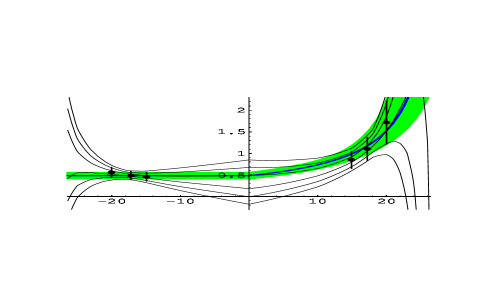
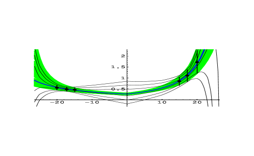
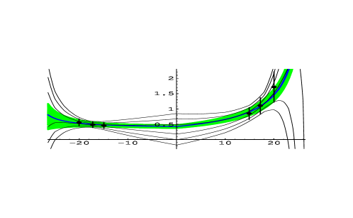
$q^{2}$

$q^{2}$

$q^{2}$

$f^{0}(|q^{2}|)$

$f^{0}(|q^{2}|)$

$f^{0}(|q^{2}|)$

$f^{+}(q^{2})$

$f^{+}(q^{2})$

$f^{+}(q^{2})$

$(a)$

$(b)$

$(c)$

Figure 4: $f^{0}(|q^{2}|)$ and $f^{+}(q^{2})$ versus $q^{2}$ with $q^{2}$ in $\,\mbox{GeV}^{2}$, as in Fig. 1. The data points are the lattice results of the UKQCD Collaboration [27] with additional systematic errors (see Appendix C). The pairs of fine solid curves are, from the outermost to the innermost, our 90%, 70% and 30% model-independent QCD bounds. The thick curves are the results of fits and the bands, the corresponding 68% C.L. regions, for fits to the three parametrizations described in Section 2: $(a)$ “constant/pole”; $(b)$ “pole/dipole”; $(c)$ “fixed-pole” with the pole mass fixed to $m_{B^{*}}$.

8 The Couplings $g_{B^{*}B\pi}$ and $g$

Having obtained bounds on $f^{+}(q^{2})$, we can use Eqs. (37) and (38) to constrain the $B^{*}B\pi$ coupling, $g_{B^{*}B\pi}$. Using Eq. (54) and $f_{B^{*}}=33\raisebox{0.80002pt}{\scriptsize{$\;\begin{array}[]{@{}l@{}}\makebox[15.0pt][c]{$+$}\makebox[1.04996pt][r]{4}\\[-0.83997pt] \makebox[15.0pt][c]{$-$}\makebox[1.04996pt][r]{4}\end{array}$}}$ (see comments after Eq. (52)), we find

$$-8.9\pm 1.1\leq-6.2\pm 0.8\leq-3.4\pm 0.4\leq g\leq 6.7\pm 0.8\leq 9.3\pm 1.1\leq 11.6\pm 1.4$$ (57)

and

$$-724\pm 88\leq-505\pm 61\leq-275\pm 33\leq g_{B^{*+}B^{0}\pi^{+}}\leq 544\pm 66\leq 751\pm 91\leq 942\pm 114\ ,$$ (58)

where the outer limits correspond to a CL of 95%, the next interval inward, to a CL of 70% and the smallest interval to a CL of 30%. The errors come from the uncertainties on $f_{B^{*}}$. These bounds are weak because we do not have lattice results for $f^{+}(q^{2})$ very near $q^{2}_{max}$. This will be remedied, though, as soon as the lattice calculation of Ref. [27] is repeated with a sufficient number of light quark masses to enable a numerical chiral extrapolation of the form factors (see Appendix C for details) and thus provide determinations of the form factors closer to $q^{2}_{max}$.

For completeness, we also give the results for these couplings obtained under the assumption of pure $B^{*}$ dominance. As we have seen, $B^{*}$ dominance describes the lattice results well and is consistent with our bounds. We find:

$$g=0.35\pm 0.05$$ (59)

and

$$g_{B^{*+}B^{0}\pi^{+}}=28\pm 4\ .$$ (60)

Both these results and the bounds include statistical and systematic errors since the lattice results used to obtain these results do (see Appendix C for details). However, it is important to note that only the bounds of Eqs. (57) and (58) are model-independent and that the errors quoted in Eqs. (59) and (60) do not include the possible deviation of the form factor $f^{+}(q^{2})$ from pure $B^{*}$-pole behavior. The results of Eqs. (59) and (60) must therefore be treated cautiously.

Nevertheless, the pole result for $g_{B^{*+}B^{0}\pi^{+}}$ compares very favorably with the light-cone sumrule prediction of Belyaev et al. [16] who find $g_{B^{*+}B^{0}\pi^{+}}=29\pm 3$. It is rather high, however, compared to the soft-pion sumrule result of Colangelo et al. [39], $g_{B^{*+}B^{0}\pi^{+}}=15\pm 4$, and to the QCD double-moment spectral sumrule result of Dosch et al., $g_{B^{*+}B^{0}\pi^{+}}=14\pm 4$ [40]. As pointed out in Ref. [16], the sumrule of Ref. [39] can be derived from the light-cone sumrule of Ref. [16]. Though the authors of Ref. [16] and Ref. [39] agree on the sumrule, they disagree on its evaluation, the former finding $g_{B^{*+}B^{0}\pi^{+}}=28\pm 6$ in the soft-pion limit. For a discussion of this disagreement as well as a good summary of recent determinations of $g_{B^{*}B\pi}$, please see Ref. [16].

9 Bounds on the Rate, Comparisons with other Predictions and $|V_{ub}|$

Our bounds on $f^{+}(q^{2})$ enable us to constrain the rate $d\Gamma\left(\bar{B}^{0}\to\pi^{+}\ell^{-}\bar{\nu}_{\ell}\right)/dq^{2}$. In the limit of vanishing lepton mass, which is an excellent approximation for $\ell=e,\,\mu$, we have

$$\frac{d\Gamma}{dq^{2}}(\bar{B}^{0}\to\pi^{+}\ell^{-}\bar{\nu}_{\ell})=\frac{G_{F}^{2}|V_{ub}|^{2}}{192\pi^{3}m_{B}^{3}}\,\lambda^{3/2}(q^{2})\,|f^{+}(q^{2})|^{2}\ ,$$ (61)

where $\lambda(q^{2})=(m_{B}^{2}+m_{\pi}^{2}-q^{2})^{2}-4m_{B}^{2}m_{\pi}^{2}$ and $0\leq q^{2}\leq q^{2}_{max}$.

As was done for $f^{+}(q^{2})$ and $f^{0}(q^{2})$ in Section 5, we define the minimum probability that the total rate for $\bar{B}^{0}\to\pi^{+}\ell^{-}\bar{\nu}_{\ell}$ decays takes a value inside an interval $[\Gamma_{lo},\Gamma_{up}]$. This probability is given by

$${\cal P}_{\Gamma}([\Gamma_{lo},\Gamma_{up}]|\vec{f}^{+};\vec{f}^{0})\equiv\frac{1}{Z(\vec{f}^{+};\vec{f}^{0})}\int d\mu(\vec{f}^{+};\vec{f}^{0})\,\,{\cal P}_{in}(\vec{f}^{+},\vec{f}^{0})\,\,\theta\left(\Gamma_{up}-G_{up}\left(\vec{f}^{+},f^{+}(0)\in[\phi_{lo},\phi_{up}]\right)\right)$$ (62)

$$\times\,\theta\left(G_{lo}\left(\vec{f}^{+},f^{+}(0)\in[\phi_{lo},\phi_{up}]\right)-\Gamma_{lo}\right)\ ,$$

where

$$G_{up}(\vec{f}^{+},f^{+}(0)\in[\phi_{lo},\phi_{up}])\equiv\frac{G_{F}^{2}|V_{ub}|^{2}}{192\pi^{3}m_{B}^{3}}\int_{0}^{q^{2}_{max}}dq^{2}\,\lambda^{3/2}(q^{2})$$

$$\times\quad\mbox{Max}\left\{\left|F_{up}^{+}(q^{2}|\vec{f}^{+},f^{+}(0)\in[\phi_{lo},\phi_{up}])\right|^{2}\,,\,\left|F_{lo}^{+}(q^{2}|\vec{f}^{+},f^{+}(0)\in[\phi_{lo},\phi_{up}])\right|^{2}\right\}$$ (63)

and

$$G_{lo}(\vec{f}^{+},f^{+}(0)\in[\phi_{lo},\phi_{up}])\equiv\frac{G_{F}^{2}|V_{ub}|^{2}}{192\pi^{3}m_{B}^{3}}\int_{0}^{q^{2}_{max}}dq^{2}\,\lambda^{3/2}(q^{2})$$

$$\times\quad\left\{\begin{array}[]{l}0\,,\quad\mbox{if $F_{lo}^{+}(q^{2}|\vec{f}^{+},f^{+}(0)\in[\phi_{lo},\phi_{up}])\leq 0\leq F_{up}^{+}(q^{2}|\vec{f}^{+},f^{+}(0)\in[\phi_{lo},\phi_{up}])$}\\ \mbox{Min}\left\{\left|F_{up}^{+}(q^{2}|\vec{f}^{+},f^{+}(0)\in[\phi_{lo},\phi_{up}])\right|^{2}\,,\,\left|F_{lo}^{+}(q^{2}|\vec{f}^{+},f^{+}(0)\in[\phi_{lo},\phi_{up}])\right|^{2}\right\},\quad\mbox{otherwise,}\end{array}\right.$$ (64)

where $F_{lo}^{+}(\cdots)$ and $F_{up}^{+}(\cdots)$ are the bounds on $f^{+}(q^{2})$ defined in Section 4. The above expressions for the bounds on the rate are involved because the bounds on $f^{+}(q^{2})$ can change signs with $q^{2}$.

Now, using the probability of Eq. (62), we can define $p\%$ CL bounds for the rate. To calculate this probability, we use the results of the Monte Carlo for the bounds on the form factors of Section 6. Since, again, the width of a pair of bounds is typically quite small compared to the width of the distributions for upper and lower bounds, the latter are a good guide as to the behavior of the probablility of Eq. (62). We find that these distributions are bell shaped, but definitely peaked toward lower values of the rate. Therefore, instead of considering the central $p\%$ for our defining our bounds, we resort to a different procedure. Starting at the egdes of our collection of bounds, we work our way inward toward the most probable pairs of bounds by taking steps of constant size. Because the density of bounds increases much faster as we approach the most probable pairs of bounds from below than from above, we take the upward step to be much smaller than the downward step so that the increase in bound density is more or less equal in either direction. We use $0.2|V_{ub}|^{2}\,ps^{-1}$ upward steps and $1.0|V_{ub}|^{2}\,ps^{-1}$ downward steps, because they are a good compomise between size and upward and downward balance. We then call $p\%$ bound the smallest interval obtained by taking these steps which includes at least $p\%$ of the bounds. Our results depend little on the exact size of the steps or even on the procedure. For instance, taking constant percentage steps of 2% or more on whichever side of the collection of bounds is less dense gives very similar results. In all cases, we find that this density increases until about only 30% of the bounds are left. Even though the density does continue to increase slightly beyond that point, we prefer to limit ourselves to the statement that the most probable values for the rate is somewhere within these 30% bounds. The results given by our procedure are well corroborated by the distributions of lower and upper bounds mentioned above.

We present these results in Table 2. For comparison, we also collect the predictions of various authors for the total rate. We specify the $q^{2}$-range for which their calculations are valid and the assumptions made to extend the results to all of phase space. We further provide our and their predictions for $f^{+}(0)$. The spread of results for the rate is very large, the highest and lowest predictions differing by a factor of about 7. Such a spread implies a factor of about 2.6 uncertainty in the determination of $|V_{ub}|$ and clearly shows the necessity for a completely model-independent prediction.

Reference	$\Gamma\left(\bar{B}^{0}\to\pi^{+}\ell^{-}\bar{\nu}_{\ell}\right)$	$f^{+}(0)$	Details
This work	$2.4\to 28$	$-0.26\to 0.92$	95% CL
	$2.8\to 24$	$-0.18\to 0.85$	90% CL
	$3.6\to 17$	$0.00\to 0.68$	70% CL
	$4.4\to 13$	$0.10\to 0.57$	50% CL
	$4.8\to 10$	$0.18\to 0.49$	30% CL
QM [4, (WSB)]	$7.4\pm 1.6$	$0.33\pm 0.06$	$q^{2}{=}0$; $B^{*}$ pole
QM [3, (ISGW)]	2.1	0.09	$\sim q^{2}_{max}$; exponential
QM [7, (ISGW2)]	9.6		$\sim q^{2}_{max}$; dipole
QM [6]		$0.26$	$q^{2}{=}0$
QM [8]		$0.24-0.29$	QM+$B^{*}$ pole
QM [9]	9.6–15.2	$0.29-0.46$	$q^{2}{=}0\sim 20\,\mbox{GeV}^{2}$
SR2 [10]	$14.5\pm 5.9$	$0.4\pm 0.1$	$q^{2}_{max}$; modified $B^{*}$ pole
SR$2+3$ [11]	4.5–9.0	$0.27\pm 0.05$	$q^{2}{=}0$ and $q^{2}_{max}$;
			modified $B^{*}$ pole
SR3 [13]	$3.60\pm 0.65$	$0.23\pm 0.02$	$q^{2}=0\sim 5\,\mbox{GeV}^{2}$
			$+$ $B^{*}$ pole for rate
SR3 [14]	$5.1\pm 1.1$	$0.26\pm 0.02$	$q^{2}{=}0\sim 16-20\,\mbox{GeV}^{2}$
			$+$ pole fit w/
			$m_{pole}{=}5.25(10)\,\mbox{GeV}$
LCSR [15, 16, 17]	$8.1$	$0.24-0.29$	$q^{2}{=}0\sim 15\,\mbox{GeV}^{2}$, then $B^{*}$ pole
LAT [27, (UKQCD)]†	$7\pm 1$	0.21 – 0.27	$q^{2}\simeq 15\sim 20\,\mbox{GeV}^{2}$
			$+$ “pole/dipole” fit
LAT [25, (ELC)]	$9\pm 6$	0.10–0.49	single point at $q^{2}\simeq 18\,\mbox{GeV}^{2}$
			$+$ pole w/ $m_{pole}{=}5.29(1)\,\mbox{GeV}$
LAT [26, (APE)]	$8\pm 4$	0.23–0.43	single point at $q^{2}\simeq 20.4\,\mbox{GeV}^{2}$
			$+$ pole w/ $m_{pole}{=}5.32(1)\,\mbox{GeV}$

Table 2: Comparison of different theoretical predictions for $f^{+}(0)$ and the total rate for $\bar{B}^{0}\to\pi^{+}\ell^{-}\bar{\nu}_{\ell}$ decays (in units of $|V_{ub}|^{2}\,ps^{-1}$). The results in the first row block correspond to our 95%, 90%, 70%, 50% and 30% bounds on these quantities as described in the present section and Section 6. In column 1, QM stands for quark model; SR2 for two-point function QCD spectral sumrules; SR3 for three-point function QCD spectral sumrules; LCSR for light-cone sumrules; and LAT stands for lattice. The last column specifies the range of $q^{2}$ for which the calculations are reliable and the assumptions and/or fits made to extend the results to the full kinematical range.

 

^† The value for the rate differs from the one quoted in Ref. [27]. Here, the phase space integral is performed from $q^{2}=0$ to $q^{2}_{max}=26.4\,\mbox{GeV}^{2}$ assuming flavor symmetry in the light, active and spectator quarks as discussed in Appendix C. Neither the rate nor the value of $f^{+}(0)$ include systematic errors[28].

Our bounds on $f^{+}(0)$ are not very strong and at the 70% CL they are compatible with all other predictions. As discussed in Section 6, the most probable value for $f^{+}(0)$ lies within the 30% CL bounds, i.e. in the interval $[0.20,0.48]$, which is still consistent with most predictions for $f^{+}(0)$, except the ISGW result of Ref. [3].

Our bounds on the rate, on the other hand, do make some of the other predictions quite unlikely. The ISGW model result of Ref. [3] is excluded at the 95% CL; the central value of the sumrule result of Ref. [12], at the 70% CL, and the value at the tip of the error bar, at the 50% CL. All other results are compatible with our bounds at the 70% CL, including the two lattice results of Ref. [25] and Ref. [26]. They were obtained from a single measurement of $f^{+}$ for a $q^{2}\sim 18-20\,\mbox{GeV}^{2}$, assuming $B^{*}$ dominance with $m_{B^{*}}$ taken from a lattice computation with the same gluon configurations. Though the errors are mainly statistical or due to a heavy-quark mass extrapolation of the form factors similar to the one described in Appendix C, they were made as large as possible to try to accomodate the fact that the $q^{2}$-dependence of the form factor is not determined by the calculation.

Also, for $q^{2}\neq 0$ our bounds on $f^{+}(q^{2})$ have more to say, some of which could be inferred, in a different language, from a $\chi^{2}$ analysis with the lattice data alone. Considering only central values for the predictions of other authors, we find, for instance, that the sumrule result Ref. [14] is excluded by our 70% lower bound for over one-third of the kinematical range from $q^{2}\simeq 12\,\mbox{GeV}^{2}$ to $q^{2}\simeq 22\,\mbox{GeV}^{2}$ and by the 90% lower bound from $q^{2}\simeq 15\,\mbox{GeV}^{2}$ to $q^{2}\simeq 20\,\mbox{GeV}^{2}$. The WSB model, or equivalently the lattice result of Ref. [26] , is only excluded by the 70% lower bound for less than a fifth of the kinematical range, between $q^{2}\simeq 15\,\mbox{GeV}^{2}$ and $q^{2}\simeq 21\,\mbox{GeV}^{2}$. The light-cone sumrule result of Ref. [16] agrees with our bounds extremely well since it very nearly lies within our 30% bounds for $f^{+}(q^{2})$ for all $q^{2}$. Very good agreement is also found for the light-front quark model, non-relativistic hamiltonian (NR) and harmonic oscillator wavefunction (HO) results of Ref. [9] which lie within our 50% bounds for all $q^{2}$. Furthermore, the Godfrey-Isgur (GI) result of Ref. [9] agrees well with our bounds since it very nearly lies within the 70% bounds for all $q^{2}$. However, this agreement with the results of Ref. [9] implies that the $B^{*}\pi$ contribution to the $B$-meson wavefunction, which is neglected in Ref. [9], can only become significant beyond $q^{2}\sim 20\,\mbox{GeV}^{2}$ where our bounds on $f^{+}(q^{2})$ allow much more singular behavior than that given by the results of Ref. [9]. This observation is corroborated by the light-front quark model calculations of Ref. [8], since our bounds on $f^{+}(q^{2})$ favor the result which relies on the smallest value of the coupling $g$ that these authors consider.

We have also computed the rates obtained from the fits to the lattice data of various parametrizations for the form factors performed in Section 7. The results are summarized in Table 3. As these results show, only the “pole/dipole” parametrization gives a central value for the rate which lies within our 30% bounds which, together with the observations of Section 7, indicates that, of the forms we have tried, it appears to be the most probable one. Then comes the “fixed-pole” prediction which lies within the 50% bounds and finally the “constant-pole” rate which is excluded by the 50% bounds but lies within the 70% bounds. However, once again, the bounds will have to improve before a firm conclusion as to the preferred $q^{2}$-behavior of the form factors can be drawn.

fit type	$\Gamma\left(\bar{B}^{0}\to\pi^{+}\ell^{-}\bar{\nu}_{\ell}\right)$ in units of $|V_{ub}|^{2}\,ps^{-1}$
cst/pole	$15.2+7.5-3.1$
pole/dipole	$8.5+3.0-1.9$
fixed-pole	$12.3+2.5-2.2$

Table 3: Values for the rate obtained from the fits described in Section 7. The error bars are 70% errors.

Finally, the most probable value for the rate is somewhere in the interval $[4.8,10]|V_{ub}|^{2}\,ps^{-1}$ which corresponds to the 30% CL bounds. Thus, we can summarize our results for the rate as

$$\Gamma\left(\bar{B}^{0}\to\pi^{+}\ell^{-}\bar{\nu}_{\ell}\right)=(4.8\leftrightarrow 10)\raisebox{0.80002pt}{\scriptsize{$\;\begin{array}[]{@{}l@{}}\makebox[15.0pt][c]{$+$}\makebox[6.29996pt][r]{7.0}\\[-0.83997pt] \makebox[15.0pt][c]{$-$}\makebox[6.29996pt][r]{1.2}\end{array}$}}|V_{ub}|^{2}\,ps^{-1}$$ (65)

where the errors are obtained from the 70% CL bounds. Because we have been generous in our estimate of possible systematic errors, the theoretical error in Eq. (65) is probably an overestimate and the 60% CL bounds or even perhaps the 50% CL bounds may give a better estimate of this theoretical error. For instance, the estimate given by the 50% CL bounds is:

$$\Gamma\left(\bar{B}^{0}\to\pi^{+}\ell^{-}\bar{\nu}_{\ell}\right)=(4.8\leftrightarrow 10)\raisebox{0.80002pt}{\scriptsize{$\;\begin{array}[]{@{}l@{}}\makebox[15.0pt][c]{$+$}\makebox[6.29996pt][r]{3.0}\\[-0.83997pt] \makebox[15.0pt][c]{$-$}\makebox[6.29996pt][r]{0.4}\end{array}$}}|V_{ub}|^{2}\,ps^{-1}\ .$$ (66)

Now, the CLEO Collaboration very recently measured the branching ratio for $\bar{B}^{0}\to\pi^{+}\ell^{-}\bar{\nu}_{\ell}$ decays [1]. They found

$${\cal B}\left(\bar{B}^{0}\to\pi^{+}\ell^{-}\bar{\nu}_{\ell}\right)=\left\{\begin{array}[]{ll}(1.63\pm 0.46\pm 0.34)\times 10^{-4}&\mbox{WSB}\\ (1.34\pm 0.35\pm 0.28)\times 10^{-4}&\mbox{ISGW}\end{array}\right.\ ,$$ (67)

where experimental efficiencies are determined with the WSB model [4] and the ISGW model [3], respectively. Because of the model dependence of their results, a precise statement about $|V_{ub}|$ is not yet possible. However, to illustrate the sort of accuracy our results lead to, we proceed to extract $|V_{ub}|$ from these measurements. Because our bounds favor very strongly the WSB model predictions for $f^{+}$ and the rate over those of the ISGW model, we consider only the WSB measurement. Using the result of Eq. (65), we find

$$|V_{ub}|\,\sqrt{\tau_{\bar{B}^{0}}/1.56\,ps}=(0.0032\leftrightarrow 0.0047)+0.0007-0.0007\pm 0.0007\quad\mbox{(WSB)}\ ,$$ (68)

where the first set of errors is theoretical (non-gaussian) and the second experimental (statistical and systematic combined in quadrature on the average value of $|V_{ub}|$ given by the 30% CL results). The value of $\tau_{\bar{B}^{0}}$ we have taken is $1.56(5)\,ps$ [59]. Using the less conservative result of Eq. (66) for the total rate, we find

$$|V_{ub}|\,\sqrt{\tau_{\bar{B}^{0}}/1.56\,ps}=(0.0032\leftrightarrow 0.0047)+0.0002-0.0004\pm 0.0007\quad\mbox{(WSB)}\ ,$$ (69)

where the origin of the errors is the same as in Eq. (68). Finally, using the 90% CL bounds on the rate, we get

$$0.0021\pm 0.0004\leq|V_{ub}|\,\sqrt{\tau_{\bar{B}^{0}}/1.56\,ps}\leq 0.0061\pm 0.0011\quad\mbox{(WSB)}\ ,$$ (70)

and using the the 95% CL bounds,

$$0.0019\pm 0.0003\leq|V_{ub}|\,\sqrt{\tau_{\bar{B}^{0}}/1.56\,ps}\leq 0.0066\pm 0.0012\quad\mbox{(WSB)}\ ,$$ (71)

where the errors shown on the bounds are the experimental errors.

The determination of $|V_{ub}|$ given in Eq. (68) has a theoretical error of 37%, computed by taking the difference of the 70% CL bound results over their sum. Though this error is by no means negligible, it is nevertheless quite reasonable especially since the result of Eq. (68) is completely model-independent and is obtained from lattice data which include a conservative range of systematic errors (please see Appendix C for details). The determination of $|V_{ub}|$ given in Eq. (69), obtained under less conservative assumptions (i.e. from the 50% CL bounds), has a theoretical error of 27%.

10 Conclusion

We have combined lattice results, a kinematical constraint and QCD dispersion relations to derive model-independent bounds on the form factors relevant for semileptonic $\bar{B}^{0}\to\pi^{+}\ell^{-}\bar{\nu}_{\ell}$ decays. Even though the contribution of the form factor $f^{0}$ to the rate is negligible, we have found its bounds useful for constraining $f^{0}(0)=f^{+}(0)$, thereby making the bounds on $f^{+}(q^{2})$ stronger. And although our bounds do not unambiguously exclude any of the parametrizations for the $q^{2}$-dependence of the form factors that we have tried, they do limit the range of possible parameter values and indicate that some of the parametrizations are more probable than others. We find, for instance, that the “pole-dipole” parametrization of Section 2 appears to be more likely than the “fixed-pole” parametrization which, in turn, appears more probable that the “constant-pole” parametrization. We also find excellent agreement with the light-cone sumrule results of Ref. [16] for $f^{+}(q^{2})$ which almost lie within our 30% bounds for all $q^{2}$. Agreement with our bounds for $f^{+}(q^{2})$ is also very good for the non-relativistic hamiltonian (NR) and the harmonic oscillator wavefunction (HO) results of the light-front quark model calculations of Ref. [9] which both lie within our 50% bounds for all $q^{2}$. Further good agreement is found with the Godfrey-Isgur (GI) result of Ref. [9] which very nearly lies within our 70% bounds for all $q^{2}$. This agreement with the results of Ref. [9] implies that the $B^{*}\pi$ contribution to the $B$-meson wavefunction, which is neglected in Ref. [9], can only become significant beyond $q^{2}\sim 20\,\mbox{GeV}^{2}$ where our bounds on $f^{+}(q^{2})$ allow much more singular behavior than that given by the results of Ref. [9]. Agreement of other predictions with our bounds ranges from slightly less good to much less good. However, the bounds will have to improve before a firm conclusion as to the preferred $q^{2}$-behavior of the form factors can be drawn.

We also use our bounds, as well as the vector dominance results, to determine the $B^{*}B\pi$ coupling and the coupling $g$ which appears in Heavy-Meson Chiral lagrangians at leading order. While our bounds on these couplings are quite weak, our “fixed-pole” fit to the form factors yields $g=0.35\pm 0.05$ (Eq. (59)) and $g_{B^{*+}B^{0}\pi^{+}}=28\pm 4$ (Eq. (60)). It is important to note, however, that the “fixed-pole” results rely on the assumption that $f^{+}$ is dominated by the $B^{*}$ pole over the full kinematical domain.

We further derive bounds on the total rate. These bounds disfavor some quark model and sumrule predictions with some certainty. At the 70% CL, they also enable the extraction of $|V_{ub}|$ from the corresponding experimental results with a theoretical error of 37%. Since we have been generous in our estimate of possible systematic errors, this 37% is probably an overestimate. It can be reduced to 27% if one is willing to accept the 50% CL bounds as a good estimate of the theoretical uncertainties. More generally, this extraction is complementary to the lattice determination of $|V_{ub}|$ from the differential decay rate for $\bar{B}^{0}\to\rho^{+}\ell^{-}\bar{\nu}_{\ell}$ decays suggested in [58]. Furthermore, the preliminary determination of the branching ratio for $\bar{B}^{0}\to\pi^{+}\ell^{-}\bar{\nu}_{\ell}$ decays by the CLEO collaboration [1] suffers from a rather strong model dependence. Perhaps this model dependence could be reduced by using our results.

As mentioned in the Introduction and described in Appendix C, we assume flavor symmetry in the light, active and spectator quarks in using the UKQCD Collaboration lattice results of Ref. [27] for $f^{+}(q^{2})$ and $f^{0}(q^{2})$. Although there is evidence that such a symmetry is reliable for the values of $q^{2}$ we consider, we add large systematic errors to the data to cover possible violations. We further add a very large range of errors to account for other possible systematic effects. With these systematic errors (and in some cases even without) the lattice results of Table 6 are compatible with the very few chirally extrapolated points of Refs. [25] and [26] within one standard deviation or less. Of course, our whole analysis should be repeated once a complete set of reliable chirally extrapolated results are available.

We add all of these systematic errors to the lattice results before performing our analysis. We believe that such a procedure is sensible in phenomenological applications when systematic uncertainties dominate over statistical ones. As discussed in the Introduction and in Section 7 this gives a more conservative representation of the accuracy of the lattice results. We are thus confident that our final results are correct within these large errors.

We have also investigated the effect of reducing lattice errors. With errors reduced by a factor 4, the corresponding lattice constrained bounds would certainly discriminate amongst various parametrizations and would enable an extraction of $|V_{ub}|$ from the experimental branching ratio with a theoretical error of about 20%. A more effective means of improving the bounds, however, would be lattice results over a wider range of $q^{2}$. This range will increase as simulations on finer lattices become available. Of course, a reliable determination of the form factors at or around $q^{2}=0$ would help tremendously. We refrained, in the present paper, from using sumrule or quark model results around $q^{2}=0$ because the systematic errors of these calculations are so different from those of the lattice. We wanted to keep the results model-independent and wished to explore the extent to which the lattice alone could constrain $\bar{B}^{0}\to\pi^{+}\ell^{-}\bar{\nu}_{\ell}$ decays. In the future, however, one may want to use the methods developed here to combine results for the relevant form factors obtained by different methods in different kinematical regimes.

For the quantities which depend on knowing the $q^{2}$-dependence of the form factors close to $q^{2}_{max}$, such as the $B^{*}B\pi$ couplings or partially integrated rates above the charm production endpoint, significant improvement in accuracy can be achieved by simply repeating the simulation which led to the results of Ref. [27] with a sufficient number of light quark masses to enable a numerical chiral extrapolation of the form factors (see Appendix C for details) and thus provide determinations of the form factors closer to $q^{2}_{max}$.

We have also performed an analysis of the QCD corrections–both perturbative and non-perturbative–to the relevant polarization functions so as to determine the range of $Q^{2}$ in which one may trust the QCD evaluation of these functions. We have found that these corrections are under control at $Q^{2}=0$ but not at $Q^{2}=-16\,\mbox{GeV}^{2}$.

Finally, the methods developed here to take into account the kinematical constraint and errors on the lattice results are completely general. They can be used with sumrule or quark model results to extend these results to kinematical regimes where these calculations break down. Furthermore, our methods are, in principle, applicable to other processes of great physical interest such as the rare decay $\bar{B}\to K^{*}\gamma$, where a model-independent guide for extrapolating the lattice results for the relevant form factor from $q^{2}$ around $q^{2}_{max}$ to $q^{2}=0$ is urgently needed, or to the semileptonic decay $\bar{B}\to\rho\ell\bar{\nu}$ which would enable an independent determination of $|V_{ub}|$. Also, as a by-product of implementing the kinematical constraint, we have derived a formalism which enables one to constrain bounds on a form factor with the knowledge that it must lie within an interval of values at one or more values of $q^{2}$. More generally, we believe that the combination of lattice results with dispersive techniques will lead to many more interesting results in the future.

Acknowledgements

I would like to thank the UKQCD Collaboration and in particular the authors of Ref. [27] for sharing their results with me. I would like to thank Eduardo de Rafael, Irinel Caprini, Jonathan Flynn, Lawrence Gibbons, Thomas Mannel, Stephan Narison, Juan Nieves and Jay Watson for useful discussions. Eduardo de Rafael, Jonathan Flynn and Juan Nieves are further thanked for reading the manuscript with care. I wish also to thank Alexander Khodjamirian for pointing out a discrepancy between the normalization convention for $g_{B^{*}B\pi}$ used in an earlier draft of this paper and the standard convention and for elaborating on some of the results in Refs. [15] and [16]. Finally, I gratefully acknowledge the hospitality of the Service de Physique Théorique de Saclay and of the Benasque School for Physics where part of this work was done.

Appendix A Explicit Expressions for the Bounding Functions

Consider the positive semi-definite, $(L+1)\times(L+1)$ matrix

$$M(\vec{f})=\left(\begin{array}[]{ccccc}\langle\phi f|\phi f\rangle&\langle\phi f|g_{t_{1}}\rangle&\langle\phi f|g_{t_{2}}\rangle&\cdots&\langle\phi f|g_{t_{L}}\rangle\\ \langle g_{t_{1}}|\phi f\rangle&\langle g_{t_{1}}|g_{t_{1}}\rangle&\langle g_{t_{1}}|g_{t_{2}}\rangle&\cdots&\langle g_{t_{1}}|g_{t_{L}}\rangle\\ \langle g_{t_{2}}|\phi f\rangle&\langle g_{t_{2}}|g_{t_{1}}\rangle&\langle g_{t_{2}}|g_{t_{2}}\rangle&\cdots&\langle g_{t_{2}}|g_{t_{L}}\rangle\\ \vdots&\vdots&\vdots&\vdots&\vdots\\ \langle g_{t_{L}}|\phi f\rangle&\langle g_{t_{L}}|g_{t_{1}}\rangle&\langle g_{t_{L}}|g_{t_{2}}\rangle&\cdots&\langle g_{t_{L}}|g_{t_{L}}\rangle\end{array}\right)\ ,$$ (72)

with $\vec{f}=(f(t_{1}),\cdots,f(t_{L}))$ and all $t_{i}$ distinct. The elements of this matrix can be chosen real for $t_{1},t_{2},\cdots$ in the interval $(-\infty,t_{+})$ in which case the matrix is symmetric. Then, its determinant is

$$\det{M(\vec{f})}=\langle\phi f|\phi f\rangle\det{M(\vec{f})^{\{(1,1)\}}}-\sum^{L}_{i,j=1}a_{ij}\langle g_{t_{i}}|\phi f\rangle\langle g_{t_{j}}|\phi f\rangle$$ (73)

with

$$a_{ij}=(-1)^{i+j}\det{M(\vec{f})^{\{(1,1),(i+1,j+1)\}}}$$ (74)

where the matrix $M(\vec{f})^{\{(i_{1},j_{1},),(i_{2},j_{2}),\cdots\}}$ is the matrix obained by deleting rows $i_{1},i_{2},\cdots$ and columns $j_{1},j_{2},\cdots$ from $M(\vec{f})$.

Then,

$$\det{M(\vec{f})}\geq 0\Longrightarrow J(Q^{2})\det{M(\vec{f})^{\{(1,1)\}}}\geq\sum^{L}_{i,j=1}a_{ij}\langle g_{t_{i}}|\phi f\rangle\langle g_{t_{j}}|\phi f\rangle\ ,$$ (75)

where we have used Eq. (24) and the fact that $\det{M(\vec{f})^{\{(1,1)\}}}$ is positive because of the positivity of the inner product.

The positivity of the inner product further implies that:

• $a_{ii}>0$ for all $i=1,\cdots,L$ so that $\mbox{Tr}\;a>0$;

• $\det{a}=\left(\det{M(\vec{f})^{\{(1,1)\}}}\right)^{L-1}>0$.

Therefore, the constraint of Eq. (75) requires $\vec{f}$ to lie within the $L$-dimensional volume in $\vec{f}$-space delimited by the $L-1$-dimensional ellipsoid centered at the origin and defined by the equality in Eq. (75) ($\phi(z(t),Q^{2})$ is chosen real and positive for all $t<t_{+}$). One can further show that this ellipsoid is circumscribed by the box whose sides are given by the hyperplanes which are solutions to the $L$ equations $\det{M(f_{i})}=0$, $i=1,\cdots,L$. What this means is that the maximum and minimum values that any of the $f(t_{i})$ can take inside this ellipsoid are given by the unconstrained bounds of Eq. (28) with $t=t_{i}$.

Now, suppose that we wish to find the bounds that Eq. (75) imposes on $f(t_{1})$ given $f(t_{2}),\cdots,f(t_{L})$. Eq. (75) can be rewritten as

$$\gamma\geq\alpha\langle g_{t_{1}}|\phi f\rangle^{2}+2\beta\langle g_{t_{1}}|\phi f\rangle$$ (76)

with

$$\alpha = a_{11}\ ,$$

$$\beta = \sum_{i=2}^{L}a_{1i}\langle g_{t_{i}}|\phi f\rangle\ ,$$

$$\mbox{and}\quad\gamma = J(Q^{2})\,\det{M(\vec{f})^{\{(1,1)\}}}-\sum^{L}_{i,j=2}a_{ij}\langle g_{t_{i}}|\phi f\rangle\langle g_{t_{j}}|\phi f\rangle\ .$$ (77)

One can show that the discriminant of the quadratic inequality of Eq. (76) is

$$\Delta=\det{M(\vec{f})^{\{(1,1)\}}}\,\det{M(\vec{f})^{\{(2,2)\}}}\ ,$$ (78)

where $M(\vec{f})^{\{(2,2)\}}=M(f(t_{2}),\cdots,f(t_{L}))$. Since $\det{M(\vec{f})^{\{(1,1)\}}}\geq 0$, Eq. (76) will have a solution iff $(f(t_{2}),$ $\cdots,$ $f(t_{L}))$ themselves satisfy the dispersive constraint $\det{M(f(t_{2}),\cdots,f(t_{L}))}\geq 0$. If this is the case, we find that

$$F_{lo}(t_{1}|f(t_{2}),\cdots,f(t_{L}))\leq f(t_{1})\leq F_{up}(t_{1}|f(t_{2}),\cdots,f(t_{L}))\ ,$$ (79)

with

$$F_{lo/up}(t_{1}|f(t_{2}),\cdots,f(t_{L}))={-\beta\,-{/}+\,\sqrt{\Delta}\over\alpha}\ ,$$ (80)

since $\alpha=a_{11}>0$. The bounds of Eq. (31) in Section 3 correspond to those of Eqs. (79) and (80) with $L=N+1$ and with the replacements $t_{1}\to t$ and $t_{i}\to t_{i-1}$, $i=2,\cdots,N+1$.

Now, to impose the kinematical constraint of Eq. (2) we need to know how the bounds $F_{lo}(t|\vec{f},x)$ and $F_{up}(t|\vec{f},x)$ behave as a function of $x$, with $\vec{f}=(f(t_{1}),\cdots,f(t_{N}))$ fixed and $x=f(t_{N+1})$. These bounds are obtained from the condition $\det{M(f(t),\vec{f},x)}\geq 0$. The results of this appendix imply that the bounds $F_{lo}(t|\vec{f},x)$ and $F_{up}(t|\vec{f},x)$ exist iff $\det{M(\vec{f},x)}\geq 0$. This in turn means that $x$ is constrained to the interval $[x_{lo},x_{up}]$ with $x_{lo(up)}=F_{lo(up)}(t_{N+1}|\vec{f})$.

Furthermore, because the condition $\det{M(f(t),\vec{f},x)}\geq 0$ implies that $(f(t),\vec{f},x)$ must lie on an $N+1$-dimensional ellipsoid, $F_{lo(up)}(t|\vec{f},x)$, viewed as a function of $x$ with $t$ and $\vec{f}$ fixed, must be the lower (upper) segment of an ellipse bisected by the line that goes through the points $(x_{lo},F_{lo}(t|\vec{f},x_{lo})$$=$$F_{up}(t|\vec{f},x_{lo}))$ and $(x_{up},F_{lo}(t|\vec{f},x_{up})$$=$$F_{up}(t|\vec{f},x_{up}))$. Since the tangents to the ellipse at these points are vertical, $F_{up}(t|\vec{f},x)$ must increase monotically with $x$ from $x=x_{lo}$ to $x=x_{max}$ where it reaches its maximum value and then decrease monotically until $x=x_{up}$ beyond which it is not defined. Similarly, $F_{lo}(t|\vec{f},x)$ decreases monotically with $x$ from $x=x_{lo}$ to $x=x_{min}$ where it reaches its minimum value and then increases monotically until $x=x_{up}$ beyond which it is not defined. Moreover, one can show that $F_{up}(t|\vec{f},x_{max})=F_{up}(t|\vec{f})$, i.e. the bounds one would obtain without any constraints on $x=f(t_{N+1})$. Simlarly, $F_{lo}(t|\vec{f},x_{min})=F_{lo}(t|\vec{f})$.

Appendix B The Functions $\chi_{T,L}(Q^{2})$ in QCD

To quantify the ${\cal O}\left(\alpha_{s}\right)$ corrections to the polarization function, $\Pi^{\mu\nu}(q)$, we use the results of Ref. [42, 43]. Because the mass of the $b$ quark, $m_{b}$, appears already at 1-loop order, the relative size of this leading contribution and the ${\cal O}\left(\alpha_{s}\right)$ correction will depend on the renormalization scheme used for this mass. The calculations of Ref. [42, 43] were peformed using an on-shell scheme. To test the reliability of these calculations as $Q^{2}$ is changed, we perform them in two additional schemes. Thus, the three schemes are:

• pole:

  • $m_{b}=m_{b}^{pole}$

  • $\alpha_{s}(\mu)$ in $\overline{\mbox{MS}}$-scheme

  • $\mu=\sqrt{Q^{2}+m_{b}^{2}}$

• $\overline{\mbox{MS}}$:

  • $m_{b}=\overline{m_{b}}(\mu)$ with $m_{b}^{pole}=m_{b}\left(1+\frac{\alpha_{s}(\mu)}{\pi}\phi(\mu)\right)$ and $\phi(\mu)=\mbox{ln}\left(\frac{\mu^{2}}{m_{b}^{2}}\right)+\frac{4}{3}$

  • $\alpha_{s}(\mu)$ in $\overline{\mbox{MS}}$-scheme

  • $\mu=\sqrt{Q^{2}+m_{b}^{2}}$

• euclidean (Landau gauge):

  • $m_{b}=m_{b}^{euc}(\mu)$ with $m_{b}^{pole}=m_{b}\left(1+\frac{\alpha_{s}(\mu)}{\pi}\phi(\mu)\right)$ and $\phi(\mu)=-\frac{\mu^{2}+m_{b}^{pole}}{\mu^{2}}\mbox{ln}\left(\frac{\mu^{2}+m_{b}^{pole}}{(m_{b}^{pole})^{2}}\right)$

  • $\alpha_{s}(\mu)$ in $\overline{\mbox{MS}}$-scheme

  • $\mu=\sqrt{Q^{2}+(m_{b}^{pole})^{2}}$.

$\mu=\sqrt{Q^{2}+m_{b}^{2}}$ is a natural scale for this process and, obviously, $\phi\equiv 0$ in the pole scheme.

The non-perturbative corrections, which are due to interactions of the $b$ and $\bar{u}$ quarks with quark and gluons condensates, can be evaluated with the standard diagrammatic techniques of Ref. [44] or with background field methods as in Ref. [45]. Using the diagrammatic techniques, we have checked the results of Ref. [43, 45] for condensates of dimensions 3 and 4. Combining all of these results and keeping contributions of condensates with dimension less or equal to 4, we find (setting $m_{u}=0$)

$$\chi_{L}(Q^{2}) = \frac{1}{\pi m_{b}^{2}}\int_{0}^{1}dx\,\frac{\left(m_{b}^{2}/x\right)\,\mbox{Im}\,\Pi_{L}^{pert}(x)}{\left(1+(Q^{2}/m_{b}^{2})x\right)^{2}}$$ (81)

$$+\frac{\bar{m}_{b}(1\,\mbox{GeV})\langle\bar{u}u\rangle_{1\,\mbox{GeV}}}{(Q^{2}+m_{b}^{2})^{2}}+\frac{1}{(Q^{2}+m_{b}^{2})^{2}}\langle\frac{\alpha_{s}}{12\pi}G^{2}\rangle\ ,$$

with

$$\left(m_{b}^{2}/x\right)\ \mbox{Im}\,\Pi_{L}^{pert}(x) = \frac{3m_{b}^{2}}{8\pi}(1-x)^{2}\left\{1+\frac{4\alpha_{s}}{3\pi}\left(\frac{9}{4}+2l(x)+\mbox{ln}\left(x\right)\mbox{ln}\left(1-x\right)\right.\right.$$ (82)

$$\left.\left.+\left(\frac{5}{2}-x-\frac{1}{1-x}\right)\mbox{ln}\left(x\right)+\left(x-\frac{5}{2}\right)\mbox{ln}\left(1-x\right)+3\phi(\mu)\frac{Q^{2}x}{m_{b}^{2}+Q^{2}x}\right)\right\}\ ,$$

and

$$\chi_{T}(Q^{2}) = \frac{1}{\pi m_{b}^{2}}\int_{0}^{1}dx\,\frac{\mbox{Im}\,\Pi_{T}^{pert}(x)}{\left(1+(Q^{2}/m_{b}^{2})x\right)^{3}}$$ (83)

$$-\frac{\bar{m}_{b}(1\,\mbox{GeV})\langle\bar{u}u\rangle_{1\,\mbox{GeV}}}{(Q^{2}+m_{b}^{2})^{3}}-\frac{1}{(Q^{2}+m_{b}^{2})^{3}}\langle\frac{\alpha_{s}}{12\pi}G^{2}\rangle\ ,$$

with

$$\mbox{Im}\,\Pi_{T}^{pert}(x) = \frac{1}{8\pi}(1-x)^{2}\left\{(2+x)+\frac{4\alpha_{s}}{3\pi}\left[(2+x)\left(\frac{13}{4}+2l(x)+\mbox{ln}\left(x\right)\mbox{ln}\left(1-x\right)+\frac{3}{2}\mbox{ln}\left(\frac{x}{1-x}\right)\right.\right.\right.$$ (84)

$$\left.-\mbox{ln}\left(1-x\right)-x\mbox{ln}\left(\frac{x}{1-x}\right)-\frac{x}{1-x}\mbox{ln}\left(x\right)\right)$$

$$-\left((3+x)(1-x)\mbox{ln}\left(\frac{x}{1-x}\right)+\frac{2x}{(1-x)^{2}}\mbox{ln}\left(x\right)+5+2x+\frac{2x}{1-x}\right)$$

$$\left.\left.+\frac{3}{2}\phi(\mu)\frac{2Q^{2}x-m_{b}^{2}}{m_{b}^{2}+Q^{2}x}\right]\right\}\ .$$

In Eqs. (82) and (84), $l(x)$ is a dilogarithm.

We have evaluated the expressions of Eqs. (81) and (83) for two values of $Q^{2}$ to investigate the range of validity of the QCD calculation. One might like to take $Q^{2}$ close to the resonance region because the strength of the bounds may increase as $Q^{2}$ approaches this region as suggested by Eqs. (16), (17), (18) and (19). We have chosen $Q^{2}=0$, which is the value traditionally used when dealing with current correlators involving a heavy quark, and $Q^{2}=-16\,\mbox{GeV}^{2}$ as was suggested in Ref. [30]. For the masses, we use the results of Ref. [46] ($\bar{m}_{b}(\bar{m}_{b})=4.3\,\mbox{GeV}$) and for the condensates:

$$\langle\bar{u}u\rangle_{1\,\mbox{GeV}}=(-0.24\,\mbox{GeV})^{3}$$

$$\langle\frac{\alpha_{s}}{\pi}G^{2}\rangle=0.02(1)\,\mbox{GeV}^{4} \ ,$$ (85)

where the quark condensate is taken from [14] and the gluon condensate, from [48]. Our results for the different contributions to $\chi_{L}(Q^{2})$ and $\chi_{T}(Q^{2})$ are summarized in Table 4 and Table 5, respectively.

	$\chi_{L}(Q^{2})$
$Q^{2}$	$0\,\mbox{GeV}^{2}$			$-16\,\mbox{GeV}^{2}$
scheme	pole	$\overline{\mbox{MS}}$	Euclid.	pole	$\overline{\mbox{MS}}$	Euclid.
1-loop	$1.3\,\times\,10^{-2}$	$1.3\,\times\,10^{-2}$	$1.3\,\times\,10^{-2}$	$2.1\,\times\,10^{-2}$	$2.1\,\times\,10^{-2}$	$2.6\,\times\,10^{-2}$
${\cal O}\left(\alpha_{s}\right)$/1-loop	16%	17%	16%	35%	32%	12%
total pert.	$1.5\,\times\,10^{-2}$	$1.5\,\times\,10^{-2}$	$1.5\,\times\,10^{-2}$	$2.8\,\times\,10^{-2}$	$2.8\,\times\,10^{-2}$	$2.9\,\times\,10^{-2}$
$m_{u}\langle\bar{u}u\rangle$/1-loop	-1%	-2%	-2%	-11%	-10%	-66%
$\langle\alpha_{s}G^{2}\rangle$/1-loop	$0.03\%$	$0.04\%$	$0.04\%$	$0.2\%$	$0.2\%$	$1.2\%$
total	$1.5\,\times\,10^{-2}$	$1.5\,\times\,10^{-2}$	$1.4\,\times\,10^{-2}$	$2.6\,\times\,10^{-2}$	$2.6\,\times\,10^{-2}$	$1.2\,\times\,10^{-2}$

Table 4: Perturbative and non-perturbative contributions to the subtracted polarization function $\chi_{L}(Q^{2})$ at two values of $Q^{2}$.

	$\chi_{T}(Q^{2})$
$Q^{2}$	$0\,\mbox{GeV}^{2}$			$-16\,\mbox{GeV}^{2}$
scheme	pole	$\overline{\mbox{MS}}$	Euclid.	pole	$\overline{\mbox{MS}}$	Euclid.
1-loop	$4.2\,\times\,10^{-4}$	$5.1\,\times\,10^{-4}$	$5.1\,\times\,10^{-4}$	$1.0\,\times\,10^{-3}$	$1.0\,\times\,10^{-3}$	$2.1\,\times\,10^{-3}$
${\cal O}\left(\alpha_{s}\right)$/1-loop	25%	7%	6%	44%	38%	-40%
total pert.	$5.3\,\times\,10^{-4}$	$5.5\,\times\,10^{-4}$	$5.4\,\times\,10^{-4}$	$1.5\,\times\,10^{-3}$	$1.4\,\times\,10^{-3}$	$1.3\,\times\,10^{-3}$
$m_{u}\langle\bar{u}u\rangle$/1-loop	2%	3%	3%	33%	30%	352%
$\langle\alpha_{s}G^{2}\rangle$/1-loop	$-0.03\%$	$-0.05\%$	$-0.05\%$	$-0.6\%$	$-0.5\%$	$-6.2\%$
total	$5.3\,\times\,10^{-4}$	$5.6\,\times\,10^{-4}$	$5.6\,\times\,10^{-4}$	$1.8\,\times\,10^{-3}$	$1.7\,\times\,10^{-3}$	$8.5\,\times\,10^{-3}$

Table 5: Perturbative and non-perturbative contributions to the subtracted polarization function $\chi_{T}(Q^{2})$ at two values of $Q^{2}$.

At $Q^{2}=0$, the perturbative and non-perturbative corrections to the one-loop results for $\chi_{L}(Q^{2})$ and $\chi_{T}(Q^{2})$ are under control, especially when the perturbative $\overline{\mbox{MS}}$ and euclidean schemes are used. Moreover, there is very little scheme dependence in the total perturbative contribution and actual values of $\chi_{L}(0)$ and $\chi_{T}(0)$. Thus, the QCD calculation appears to be reliable at $Q^{2}=0$. For $Q^{2}=-16\,\mbox{GeV}^{2}$, even though the scheme dependence of the total perturbative contributions to $\chi_{L}(Q^{2})$ and $\chi_{T}(Q^{2})$ is small, the size of the ${\cal O}\left(\alpha_{s}\right)$ corrections are large and it is somewhat doubtful that the perturbative series will converge. Furthermore, the quark condensate contributions become quite large and even blow up in the euclidean scheme. So even though the values of $\chi_{L}(Q^{2})$ and $\chi_{T}(Q^{2})$ are nearly equal in the pole and $\overline{\mbox{MS}}$ schemes, one cannot really trust the various expansions at $Q^{2}=-16\,\mbox{GeV}^{2}$. We therefore restrict ourselves to $Q^{2}=0$ throughout the paper and use the $\overline{\mbox{MS}}$ results which appear to be the most convergent and which give the loosest constraint on the polarization functions at $Q^{2}=0$.

Appendix C Lattice Parameters and Discussion of Systematic Errors

The results for the form factors $f^{+}$ and $f^{0}$ presented in Table 6 were obtained by the UKQCD Collaboration from 60 quenched $SU(3)$ gauge configurations on a $24^{3}\times 48$ lattice at $\beta=6.2$ [27]. The corresponding inverse lattice spacing as determined from the string tension is $a^{-1}=2.73(5)\,\mbox{GeV}$ [49]. Heavy and light-quark propagators were obtained using an ${\cal O}\left(a\right)$-improved Sheikholeslami-Wohlert action [50] and ${\cal O}\left(a\right)$-improved currents [51].

$q^{2}\ (\,\mbox{GeV}^{2})$	$f^{+}(q^{2})$	$f^{0}(q^{2})$
14.9	$0.85\pm 0.20$	$0.46\pm 0.10$
17.2	$1.10\pm 0.27$	$0.49\pm 0.10$
20.0	$1.72\pm 0.50$	$0.56\pm 0.12$

Table 6: Lattice results for $f^{+}(q^{2})$ and $f^{0}(q^{2})$ at three values of $q^{2}$. Please see text for details on the treatment of systematic errors.

Because cutoff effects would be too large, the $b$-quark cannot be simulated directly. Therefore, the three-point functions used to determine the form factors were calculated at four values of the heavy-quark mass straddling that of the charm quark and the corresponding results for $f^{+}$ and $f^{0}$ were extrapolated in heavy-quark mass to $m_{B}$ according to Eqs. (3) and (4) allowing for linear corrections in $1/m_{B}$ and including in the errors the variations due to possible $1/m_{B}^{2}$ corrections [27]. Of the six extrapolated points in Ref. [27], we have kept only those for which the corresponding recoil $\omega$ is completely independent of the heavy-quark mass so as to limit the introduction of possible systematic effects.

To keep volume errors under control, one cannot work with arbitrarily light quarks. The strategy, then, is to perform the calculation for several values of light-quark mass around the mass of the strange and then extrapolate the results to the up and down. However, the limited number of light-quark mass values available to the authors of Ref. [27] made it impossible for them to perform a reliable chiral extrapolation. Therefore, the results presented in Table 6 were obtained with light-quark masses slightly larger than that of the strange ($\kappa_{light}=0.14144$) and light-flavor symmetry is assumed for both the active and spectator light quarks.

Dependence of $f^{+}$ and $f^{0}$ on light spectator-quark mass should be quite small. This is corroborated by the results of [52] for semileptonic $D\to K,\pi$ decays where the form factors display no statistically significant variation as the mass of the spectator quark is changed from slightly above $m_{strange}$ to zero, while holding $q^{2}$ fixed. Since it is these very same data–supplemented with results at different values of the charm quark mass–which were used in Ref. [27] to obtain the lattice results quoted here, we expect spectator-quark flavor symmetry to be reasonable. In fact, similar spectator-quark flavor symmetry is observed in the form factors which govern $\bar{B}\rightarrow K^{*}\gamma$   decays [53] and in those which govern semileptonic $\bar{B}\to\rho\ell\bar{\nu}_{\ell}$ decays [58] where it is as small as 5%. We will assume here that uncertainties associated with light-spectator-quark flavor symmetry are 10% on both form factors for all $q^{2}$. We do not expect much of a $q^{2}$-dependence in the corrections to spectator-quark flavor symmetry for $f^{+}$ since in a pole dominance scenario, which suits the data quite well, the mass of the relevant pole does not depend on the spectator’s flavor. For $f^{0}$, which has a less pronounced $q^{2}$-dependence, the situation should be even better.

For the values of $q^{2}$ considered here (see Table 6), we also expect dependence on the active light-quark mass to be reasonable. All recent lattice simulations of semileptonic $D$ decays indicate that the ratio $f^{+}_{D\to\pi}(0)/f^{+}_{D\to K}(0)$ is consistent with 1 within errors. For instance, the authors of Ref. [52] find $f^{+}_{D\to K}(0)/f^{+}_{D\to\pi}(0)=1.09\pm 0.09$. Furthermore, the author of the sumrule calculation of Ref. [54] finds that active light-quark flavor symmetry at $q^{2}=0$ is even better for semileptonic $B$ decays: $f^{+}_{D\to K}(0)/f^{+}_{D\to\pi}(0)=1.10\pm 0.01$ versus $f^{+}_{\bar{B}\to K}(0)/f^{+}_{\bar{B}\to\pi}(0)=1.01\pm 0.02$. And because of the kinematical constraint of Eq. (2), these conclusions also hold for $f^{0}(0)$. To get a measure of the size of the uncertainties associated with assuming this flavor symmetry for fixed $q^{2}$ away from 0, we suppose pole dominance for $f^{+}(q^{2})$. Such behavior is consistent with the $q^{2}$-dependence of the lattice results as well as with our bounds. Then, assuming active-quark flavor symmetry at $q^{2}=0$, we find that $f^{+}_{\bar{B}\to\pi}(q^{2})/f^{+}_{latt}(q^{2})\simeq(1-q^{2}/m^{2}_{B_{s}^{*}})/(1-q^{2}/m^{2}_{B^{*}})$ ranges from 1.04 to 1.09 for the $q^{2}$ in Table 6 and for $m_{B_{s}^{*}}=5.42\,\mbox{GeV}$ [2]. Thus, adding 4% to 9% errors to the uncertainty on active-quark flavor symmetry at $q^{2}=0$ should give a reasonable estimate of the possible errors on $f^{+}$ for $q^{2}\neq 0$. For $f^{0}$, which has a milder $q^{2}$-dependence than that given by pole dominance, we expect that the dependence on $q^{2}$ of uncertainties due to the assumption of active-quark flavor symmetry to be mild: they should be of the same order as those on $f^{0}(0)$. Now, to accomodate a possible, slight $q^{2}$-dependence of these uncertainties, as well as possible deviations from our pole parametrization for the $q^{2}$-dependence of $f^{+}$ and violations of light, active-quark flavor symmetry at $q^{2}=0$, we will assume that this symmetry holds within 10% at $q^{2}=0$. Thus, we add in quadrature to the uncertainties in $f^{+}$, errors ranging from 14 to 19% and to those in $f^{0}$, 10% errors.

The error associated with ignoring internal quark loops (i.e. quenching) is difficult to quantify. However, quenched calculations of form factors for semileptonic $D\to K,\,K^{*}$ decays (see [52] and references therein) give results in agreement with world average experimental values, while quenched calculations of the differential decay rate for semileptonic $\bar{B}\to D$ and $\bar{B}\to D^{*}$ decays agree very well with experimental data [55]. This gives us confidence that errors due to quenching for processes involving heavy-light hadrons are rather small. Moreover, the errors due to the uncertainty in the scale discussed in the next paragraph should take some of the uncertainties associated with quenching into account since quenching is in large part responsible for this scale uncertainty. Nevertheless, to account for quenching errors which are not taken into account by the scale uncertainty we add a conservative 10% error to the form factors.

In obtaining the bounds, we have assumed that the inverse lattice spacing is $a^{-1}=2.7\,\mbox{GeV}$, as is given by the $\rho$-meson mass ($a^{-1}(m_{\rho})=2.7(1)\,\mbox{GeV}$ [56]) or the string tension ($a^{-1}(\sigma)=2.73(1)\,\mbox{GeV}$ [49]) and in accordance with the choice made in [27]. Other physical quantities lead to slightly different values for the inverse lattice spacing, typically in the range $2.5\sim 2.9\,\mbox{GeV}$ for spectral quantities [56]. This uncertainty in the determination of the scale obviously leads to uncertainties in the lattice results. These errors should be relatively small, here, since the form factors are dimensionless quantities. There are, however, two places where the scale appears. The first is in expressing the heavy-light pseudoscalar masses in physical units for the heavy-quark-mass extrapolations of the form factors. The second is in the determination of $q^{2}$ in physical units, but only in so far as the scale is used to determine the mass of the final state meson (the “pion”), since we obtain $q^{2}$ from the dimensionless quantity $\omega$ through $q^{2}=m_{B}^{2}+m_{\pi}^{2}-2m_{B}m_{\pi}\omega$, using the experimental value for $m_{B}$. We have quantified these errors by using the heavy-quark-mass dependence of the form factors given in Ref. [27] and the $q^{2}$-dependences obtained in Section 7. We find that they are less than about 5% for both form factors.

Finally, there are cutoff corrections of order ${\cal O}\left(\alpha_{s}am_{Q}\right)$ and ${\cal O}\left((am_{Q})^{2}\right)$, where $m_{Q}$ is the mass of the heavy quark in the initial meson. For the heavy-quark masses and action used in Ref. [27], these lattice artefacts induce errors in the form factors which range from 5 to 10% as indicated in the study of Ref. [55]. A systematic study of similar effects is also given in [57]. Assuming, for simplicity, that these errors grow linearly with $m_{Q}$, we have estimated the size of the error induced in the value of the form factors at the scale of the $b$ quark. We have found them to be about 10%.

To summarize, the errors on the lattice results for $f^{+}$ and $f^{0}$ given in Table 6 are the quadratic sum of the statistical uncertainties given in [27]; of a 10% systematic error associated with possible corrections to spectator-quark flavor symmetry; of an error ranging from 14% to 19%, depending on $q^{2}$, to account for possible deviations from light-active-quark flavor symmetry in $f^{+}$ and a corresponding 10% error in $f^{0}$; of a 10% error associated with quenching; of a 5% error to take into account uncertainties associated with the determination of the lattice scale; and finally, of a 10% error to account for possible cutoff effects. With these systematic errors (and in some cases even without) the lattice results of Table 6 are compatible with the very few chirally extrapolated points of Refs. [25] and [26] within one standard deviation or less. Finally, because our errors include both statistical and systematic uncertainties, all of the results in the present paper incorporate a full treatment of statistical and systematic errors.

References

• [1] R. Ammar et al. (CLEO Collaboration), CLEO CONF 95-09, EPS0165, July 1995.
• [2] Particle Data Group, Phys. Rev. D50 (1994) 1173.
• [3] N. Isgur, D. Scora, B. Grinstein and M. B. Wise, Phys. Rev. D39 (1989) 799.
• [4] M. Wirbel, B. Stech and M. Bauer, Z. Phys. C29 (1985) 637.
• [5] J.G.  Körner and G.A. Schuler, Z. Phys. C38 (1988) 511; 41 (1989) 690(E).
• [6] P.J. O’Donnell, Q.P. Xu and H.K.K. Tung, Phys. Rev. D52 (1995) 3966.
• [7] D. Scora and N. Isgur, Phys. Rev. D52 (1995) 2783.
• [8] C-Y. Cheung, C-W. Hwang and W-M. Zhang, IP-ASTP-16-95 and hep-ph/9602309.
• [9] I.L. Grach, I.M. Narodetskii and S. Simula, INFN-ISS 96/4 and hep-ph/9605349.
• [10] C.A. Dominguez and N. Paver, Z. Phys. C41 (1988) 217.
• [11] A.A. Ovchinnikov, Phys. Lett. B229 (1989) 127.
• [12] S. Narison, Phys. Lett. B283 (1992) 384
• [13] S. Narison, Phys. Lett. B345 (1995) 166.
• [14] P. Ball, Phys. Rev. D48 (1993) 3190.
• [15] V.M. Belyaev, A. Khodjamirian and R. Rückl, Z. Phys. C60 (1993) 349.
• [16] V.M. Belyaev, V.M. Braun, A. Khodjamirian and R. Rückl, Phys. Rev. D51 (1995) 6177.
• [17] A. Khodjamirian and R. Rückl, talk presented by R. Rückl at “Beauty 95”, Oxford, July 1995, to appear in the proceedings, MPI-PhT/95-97, LMU 18/95 and hep-ph/9510294.
• [18] N. Isgur and M.B. Wise, Phys. Rev. D41 (1990) 151.
• [19] N. Isgur and M.B. Wise, Phys. Rev. D42 (1990) 2388.
• [20] G. Burdman and J.F. Donoghue, Phys. Lett. B280 (1992) 287.
• [21] M.B. Wise, Phys. Rev. D45 (1992) 2188.
• [22] L. Wolfenstein, Phys. Lett. B291 (1992) 177.
• [23] G. Burdman, Z. Ligeti, M. Neubert and Y. Nir, Phys. Rev. D49 (1994) 2331.
• [24] R. Akhoury, G. Sterman and Y.-P. Yao, Phys. Rev. D50 (1994) 358.
• [25] ELC Collaboration, As. Abada et al., Nucl. Phys. B416 (1994) 675.
• [26] APE Collaboration, C. R. Allton et al., Phys. Lett. B345 (1995) 513; V. Lubicz, private communication.
• [27] UKQCD Collaboration, D. R. Burford et al., Nucl. Phys. B447 (1995) 425.
• [28] D. R. Burford, private communication.
• [29] C. Bourrely, B. Machet and E. de Rafael, Nucl. Phys. B189 (1981) 157.
• [30] C. G. Boyd, B. Grinstein and R. F. Lebed, Phys. Rev. Lett. 74 (1995) 4603.
• [31] C. G. Boyd, B. Grinstein and R. F. Lebed, Nucl. Phys. B461 (1996) 493.
• [32] I. Caprini and M. Neubert, CERN-TH/95-255 and hep-ph/9603414.
• [33] C. G. Boyd and R. F. Lebed, UCSD/PTH 95-23 and hep-ph/9512363.
• [34] UKQCD Collaboration, R. M. Baxter et al., Phys. Rev. D49 (1994) 1594.
• [35] B. Grinstein and P. Mende, Nucl. Phys. B425 (1994) 451.
• [36] E. de Rafael and J. Taron, Phys. Rev. D50 (1994) 373.
• [37] S. Okubo and I-Fu Shih, Phys. Rev. D4 (1971) 2020.
• [38] L. Lellouch, E. Sather and L. Randall, Nucl. Phys. B405 (1993) 55.
• [39] R. Colangelo, F. De Fazio and G. Nardulli, Phys. Lett. B334 (1994) 175.
• [40] H. G. Dosch and S. Narison, Phys. Lett. B368 (1996) 163.
• [41] L. Lellouch in the proceedings of the $XXXIV^{th}$ Cracow School of Theorectical Physics, Acta Physica Polonica B25 (1994) 1679.
• [42] S. C. Generalis, Open Univserity preprint OUT-4102-13.
• [43] L.J. Reinders, S. Yazaki and H.R. Rubinstein, Phys. Lett. B103 (1981) 63.
• [44] M. A. Shifman, A. I. Vainshtein and V. I. Zakharov, Nucl. Phys. B147 (1979) 385.
• [45] S. C. Generalis, J. Phys. G16 (1990) 367.
• [46] S. Narison, Acta Physica Polonica B26 (1995) 687.
• [47] C. Becchi, S. Narison, E. de Rafael and F. J. Ynduráin, Z. Phys. C8 (1981) 335.
• [48] E. Braaten, S. Narison and A. Pich, Nucl. Phys. B373 (1992) 581.
• [49] UKQCD Collaboration, C. Allton et al., Nucl. Phys. B407 (1993) 331.
• [50] B. Sheikholeslami and R. Wohlert, Nucl. Phys. B259 (1985) 572.
• [51] G. Heatlie, G. Martinelli, C. Pittori, G. C. Rossi and C. T. Sachrajda, Nucl. Phys. B352 (1991) 266.
• [52] UKQCD Collaboration, K. C. Bowler et al., Phys. Rev. D51 (1995) 4905.
• [53] UKQCD Collaboration, K. C. Bowler et al., Phys. Rev. D51 (1995) 4955.
• [54] S. Narsion, Phys. Lett. B337 (1994) 163.
• [55] UKQCD Collaboration, K. C. Bowler et al., Phys. Rev. D52 (1995) 5067; L. Lellouch (for the UKQCD Collaboration) in the proceedings of the $30^{th}$ Recontres de Moriond: QCD and High Energy Hadronic Interactions, Meribel les Allues, France, 19-25 March 1995, Marseille CPT-95/P.3196 and hep-ph/9505423.
• [56] UKQCD Collaboration, C. Allton et al., Phys. Rev. D49 (1994) 474.
• [57] M. Crisafulli, V. Lubicz, G. Martinelli and A. Vladikas, Nucl. Phys. B (Proc. Suppl.) 42 (1995) 400.
• [58] UKQCD Collaboration, J. M. Flynn et al., Nucl. Phys. B461 (1996) 327.
• [59] I.J. Kroll, FERMILAB-CONF-96-032, to appear in Proceedings of the XVII International Symposium on Lepton-Photon Interactions, Beijing, China, 10-15 August 1995.