OPERATOR EXPANSION FOR HIGH-ENERGY SCATTERING

I.BALITSKY

Center for Theoretical Physics, Laboratory for Nuclear Science

Department of Physics, MIT, Cambridge 02139

ABSTRACT

I demonstrate that the leading logarithms for high-energy scattering can be obtained as a result of evolution of the nonlocal operators - straight-line ordered gauge factors - with respect to the slope of the straight line.

I Introduction

The rapid increase of the structure function $F_{2}(x,Q^{2})$ at small $x$ that is observed in DESY at HERA (see e.g. [1]) has revived interest in the problem of the high-energy behavior of QCD amplitudes. In the leading logarithmic approximation it is governed by BFKL equation [2][3][4] leading to a $\sim x^{-0.5}$ behavior of $F_{2}(x)$ which is not far from the experimental curve. Unfortunately, there are theoretical problems with the BFKL answer which make it difficult, if not impossible, to use these leading logarithmic as a description of real high-energy processes. First and foremost, the BFKL answer violates unitarity and therefore it is at best some kind of preasymptotic behavior which can be reliable only at some intermediate energies. (The true high-energy asymptotics would correspond to the unitarization of the leading logarithmic results but this is a problem where nobody has succeeded in 20 years and not because of lack of effort.)

Moreover, even at those moderately high energies where unitarization is not important, the BFKL results in QCD are not completely rigorous. Even if we start from the scattering of hard objects such as heavy quarks, then already in the leading logarithm approximation we obtain considerable contributions from the region of small momenta (large distances) where perturbative QCD is not applicable [3][4]. In other words, the hard pomeron which is believed to describe the observed small-$x$ growth of structure function $F_{2}$ interacts strongly with the soft ”old” pomeron made from non-perturbative gluons. Therefore, it is highly desirable to have a method of separation of small- and large-distance contributions to high-energy amplitudes, and the starting point here must be a properly gauge-invariant formalism for the BFKL equation.

In present paper we suggest a kind of gauge-invariant operator expansion for high-energy amplitudes. The relevant operators are gauge factors ordered along (almost) light-like lines stretching from minus to plus infinity. These “Wilson-line” gauge factors correspond to very fast quarks moving along the lines (see e.g. [5]). It turns out that the small-$x$ behavior of structure functions is governed by the evolution of these operators with respect to deviation of the Wilson lines from the light cone; this deviation serves as a kind of “renormalization point” for these operators. In this language the BFKL equation is simply the evolution equation for the Wilson-line operators with respect to the slope of the line. The gauge-invariant generalization of the BFKL equation turns out to be a nonlinear equation which contains more information than the usual BFKL equation — for example, it describes also the triple vertex of hard pomerons in QCD (cf. [6]).

Asymptotic expansions (in large momentum limits) play a vital role in QCD. Cross sections (or amplitudes) in these limits simplify drastically, and one is thereby enabled to do calculations that would otherwise be impossible. The best established of these expansions is Wilson’s operator product expansion for the $T$-product of two electromagnetic currents:

$$T{j_{\mu}(x)j_{\nu}(0)}=\sum c_{n}(x)O_{n}(0).$$ (1)

Here the coefficients $c_{n}$ contain all the singularities at $x=0$, and the operators $O_{n}$ have no dependence on $x$. Taking the expectation value of Eq. (1) in a nucleon state and then Fourier transforming gives integer moments of the factorization theorem for deep-inelastic structure functions:

$$F_{2}(x_{B},Q^{2})=\sum_{i}C_{i}(x_{B},Q^{2}/\mu^{2},\alpha_{s}(\mu^{2}))\otimes f_{i}(x_{B},\mu^{2},\alpha_{s}(\mu^{2}))+\dots.$$ (2)

Here the parton densities $f_{i}(x_{B},\mu^{2},\alpha_{s}(\mu^{2}))$ are matrix elements of light-cone operators. The dots stand for the contributions of higher twist terms, i.e., terms damped by extra powers of $1/Q^{2}$. $x_{B}$ is the Bjorken scaling variable $x_{B}=Q^{2}/2p\cdot q$, and $\mu$ is the renormalization scale.

Both Wilson’s operator product expansion and the factorization theorem can be expressed in terms of coefficient functions and operator matrix elements. This implies that a precise definition can be given to the quantities involved. In particular, there are contributions to the cross sections that come from the non-perturbative domain of large distances. The matrix element factors include these contributions, and their definitions include non-perturbative contributions.

The renormalization scale $\mu$ has the qualitative effect of separating “hard” and “soft” contributions to the cross section. Integrals over soft momenta, those much less than $\mu$, give suppressed contributions to the coefficient functions. Integrals over hard momenta, those much greater than $\mu$, give suppressed contributions to the matrix elements. Roughly speaking the coefficient functions are given by integrals over large momenta $Q^{2}>p^{2}>\mu^{2}$, while the matrix elements are given by integrals over small momenta $p^{2}<\mu^{2}$. The crucial property that enables calculations to be done easily is that the $\mu$ dependence is given by the renormalization group equations. One can set $\mu=O(Q)$ in the coefficient functions. Both these and the kernel of the renormalization group equation can then be calculated perturbatively, in powers of $\alpha_{s}(Q)$.

Let us recall how the usual Wilson expansion helps us to find the $Q^{2}$ dependence of the moments of structure functions of deep inelastic scattering. The essence is that instead of the dependence of the physical amplitude on $Q^{2}$ (in the Euclidean region, which corresponds to the moments of structure functions), we study the dependence of matrix elements of local operators on the renormalization point $\mu$. Consider the simplest Feynman diagram shown in Fig. 1.

                                   

FIG. 1.: A typical diagram for deep inelastic scattering.

At large $q$ we can expand the current quark propagator in inverse powers of $q$

$$\frac{1}{{\kern 2.5pt\kern-2.41145pt\hbox{$q$}\kern-2.41145pt\kern-2.5pt\hbox{$/$}}+{\hbox{$k$}\kern-2.76042pt\kern-2.5pt\hbox{$/$}\kern 2.76042pt\kern-2.5pt}}=\frac{1}{{\kern 2.5pt\kern-2.41145pt\hbox{$q$}\kern-2.41145pt\kern-2.5pt\hbox{$/$}}}-\frac{1}{{\kern 2.5pt\kern-2.41145pt\hbox{$q$}\kern-2.41145pt\kern-2.5pt\hbox{$/$}}}{\hbox{$k$}\kern-2.76042pt\kern-2.5pt\hbox{$/$}\kern 2.76042pt\kern-2.5pt}\frac{1}{{\kern 2.5pt\kern-2.41145pt\hbox{$q$}\kern-2.41145pt\kern-2.5pt\hbox{$/$}}}+\frac{1}{{\kern 2.5pt\kern-2.41145pt\hbox{$q$}\kern-2.41145pt\kern-2.5pt\hbox{$/$}}}{\hbox{$k$}\kern-2.76042pt\kern-2.5pt\hbox{$/$}\kern 2.76042pt\kern-2.5pt}\frac{1}{{\kern 2.5pt\kern-2.41145pt\hbox{$q$}\kern-2.41145pt\kern-2.5pt\hbox{$/$}}}{\hbox{$k$}\kern-2.76042pt\kern-2.5pt\hbox{$/$}\kern 2.76042pt\kern-2.5pt}\frac{1}{{\kern 2.5pt\kern-2.41145pt\hbox{$q$}\kern-2.41145pt\kern-2.5pt\hbox{$/$}}}+...$$ (3)

where $n^{th}$ term of the expansion corresponds to the $n^{th}$ moment of the structure function. Unfortunately, after the expansion the loop integrals over $k$ become UV divergent so we must modify our Taylor series (3) somehow. To this end, we note that each term on the right-hand side of Eq. (3) corresponds to the matrix element of a certain quark operator of the type $\bar{\psi}(\partial_{\mu})^{n}\gamma_{\nu}\psi$; the UV divergence reflects merely the large dimensions of these operators. It is well known how to regularize these UV divergences — we must introduce the regularized operators normalized at some point $\mu$ and expand our physical amplitudes in a series of these regularized operators. Roughly speaking, each term on the right of Eq. (3) will be integrated over $k$ only up to $k=\mu$. The dependence on $\mu$ will be cancelled : in the next order in $\alpha_{s}$ the coefficients of the Taylor expansion will be modified also — they will contain terms $\sim\alpha_{s}\ln{Q^{2}\over\mu^{2}}$ which will cancel the dependence of matrix elements of the (renormalized) local operators on $\mu^{2}$. In the leading logarithmic approximation we can simply take $\mu^{2}=Q^{2}$ and the dependence of moments of structure functions on $Q^{2}$ will reflect the dependence of the matrix elements of the operators $\bar{\psi}\nabla_{\mu_{1}}...\nabla_{\mu_{n-1}}\gamma_{\mu_{n}}\psi$ on the normalization point. This dependence is given by renormalization-group equation (see e.g. the book [7]).

Summarizing, in order to find the dependence of the structure functions of deep inelastic scattering at large $Q^{2}$ we perform the following steps: (i) formally expand in inverse powers of $Q^{2}$, (ii) regularize the obtained UV divergent matrix elements of local operators, and (iii) write down (and solve) the evolution equation with respect to the normalization point $\mu$. In the original Feynman diagrams for structure functions of deep inelastic scattering the photon virtuality $Q^{2}$ plays the role of a “physical” cutoff for the integrals over loop momenta. After expansion in powers of $1/Q^{2}$ these integrals became UV divergent; by adding counterterms in the usual way we introduce an “artificial” cutoff $\mu^{2}$ for these loop integrals. Now, instead of studying of the $Q^{2}$ behavior of the original Feynman diagrams, we should trace the dependence of the matrix elements of the operators on the cutoff $\mu^{2}$. This is a lot easier thing to do because it is governed by renormalization group.

Now, we would like to generalize these ideas for high-energy scattering. In order to find the high-energy behavior of a certain physical amplitude (say, the structure function of deep inelastic scattering at very small $x$), we will perform the same three steps: (i) formally expand the amplitude at large energy $s$ — after that we will have the divergences in the longitudinal integrals, (ii) regularize these longitudinal divergences by introducing a certain cutoff, and (iii) find (and hopefully solve) the evolution equations with respect to this cutoff. As in the case of Wilson expansion, the dependence of the relevant matrix elements on the cutoff determines the high-energy behavior of the original amplitude. In the subsequent three Sections we will perform these steps. In the Appendices we present the shock-wave picture of high-energy scattering in the virtual photon frame.

II High Energy Limit

As an example, let us consider the high-energy behavior of the forward scattering amplitude for virtual photons in the region where $s=(p_{A}+p_{B})^{2}\gg p_{A}^{2},p_{B}^{2}$:

$${\cal A}(p_{A},p_{B})=-ie^{A}_{\mu}e^{A}_{\nu}e^{B}_{\xi}e^{B}_{\eta}\int\!d^{4}x\,d^{4}y\,d^{4}z\,e^{ip_{A}\cdot x+ip_{B}\cdot y}\mbox{$\langle 0|$}T\{j^{\mu}(x+z)j^{\nu}(z)j^{\xi}(y)j^{\eta}(0)\}\mbox{$|0\rangle$}.$$ (4)

(Only the connected part of the Green function is used, and the vectors $e^{A}_{\mu}$ and $e^{B}_{\mu}$ are the polarizations of the photons.) For simplicity, we assume that the virtualities of photons are negative, since then our amplitude (4) will have only one discontinuity corresponding to the total cross section of virtual photon scattering. (At $s\gg p_{A}^{2}\gg p_{B}^{2}$ this will be the cross section of deep inelastic scattering from a virtual photon at small $x$.) A typical graph is shown in Fig. 2. Our aim is to obtain the leading contribution (in powers of $s$) from graphs for the amplitude, and it is well known that the leading large-energy asymptotic behavior ($s$ times logarithms of $s$) corresponds to diagrams with gluon exchanges.

                                   

FIG. 2.: High-energy scattering of virtual photons.

To orient the reader in our subsequent technical treatment, we first explain the qualitative features of the process in coordinate space. Suppose that we view the process as one of the incoming photons, $A$ say, travelling through the color field due to the other. Because of time dilation and Lorentz contraction, each beam particle may be viewed as a collection of fast-moving, point-like objects distributed over the transverse plane. The probability of a large momentum transfer $Q$ is of order $1/Q^{2}$, so that the partons are to be regarded as travelling along straight lines while they are crossing the non-trivial part of the field. This is, of course, the parton model. In a lowest order approximation, such as Fig. 2, the partons in question are given by a single quark-antiquark pair. The photon has fluctuated to a state of a quark-antiquark pair, and this state is almost unchanged while the pair traverses the field, since the time-scale for the evolution of the state is much longer than the time to cross the field.

Another view of the same situation can be obtained in the rest frame of the beam. The field of the other particle is Lorentz contracted, time dilated (and intensified). It looks like a shock wave of width $L\sim|p_{B}^{2}|/s$, and the quarks of the beam cannot make a significant movement in the transverse direction during that time. Here, $L$ is the typical length scale of the field.

From either viewpoint, we see that the situation is one in which some version of the eikonal approximation is valid. That is, the effect of the field on the state of the quark-antiquark pair is given by integrals over the gluon field along the (straight-line) trajectories of the partons. Indeed, we will see that what we need are exactly path-ordered exponentials of the gluon field. Unlike the simple eikonal approximation, the field affects both the phase and the color orientation of the state.

A Amplitude as integral over gluon field

As usual, at high energies it is convenient to use a decomposition in Sudakov variables. For the momenta we write the standard formula

$$p^{\mu}~{}=~{}\alpha_{p}p_{1}^{\mu}+\beta_{p}p_{2}^{\mu}+p_{\perp}^{\mu},$$ (5)

where $p_{1}^{\mu}\simeq p_{A}^{\mu}-\frac{p_{A}^{2}}{s}p_{B}^{\mu}$ and $p_{2}^{\mu}\simeq p_{B}^{\mu}-\frac{p_{B}^{2}}{s}p_{A}^{\mu}$ are light-like vectors close to $p_{A}$ and $p_{B}$ respectively. (Then $g_{\mu\nu}=\frac{2}{s}(p_{1\mu}p_{2\nu}+p_{1\nu}p_{2\mu})+g^{\perp}_{\mu\nu}$.) These variables are essentially identical to light-front coordinates, $\alpha=p_{+}/\sqrt{s},{}~{}\beta=p_{-}/\sqrt{s}$. For the coordinates we use a slightly different form

$$z^{\mu}~{}=~{}\frac{2}{s}z_{*}p_{1}^{\mu}+\frac{2}{s}z_{{}_{\bullet}}p_{2}^{\mu}+z_{\perp}^{\mu},$$ (6)

where $z_{{}_{\bullet}}\equiv z_{\mu}p_{1}^{\mu}$ and $z_{*}\equiv z_{\mu}p_{2}^{\mu}$. One advantage of these coordinates is their simple scaling properties when we take the high energy limit, as in Eq. (28), below. The factors $2/s$ in the formula for the components, Eq. (6), avoid extra factors of $s$ in the combination $p\cdot z$ $=$$\alpha_{p}z_{{}_{\bullet}}+\beta_{p}z_{*}-p_{\perp}\cdot z_{\perp}$.

The Jacobian of the transition to Sudakov variables is $s/2$ so that

$$\int\!d^{4}z={2\over s}\int\!dz_{\bullet}dz_{*}d^{2}z_{\perp}~{},~{}~{}~{}\int\!d^{4}p={s\over 2}\int\!d\alpha_{p}d\beta_{p}d^{2}p_{\perp}.$$ (8)

To put the scattering amplitude (4) in a form symmetric with respect the top and bottom photons, we make a shift of the coordinates in the currents by $(z_{\bullet},0,0_{\perp})$ and then reverse the sign of $z_{\bullet}$. This gives:

$${\cal A}(p_{A},p_{B}) = -ie^{A}_{\mu}e^{A}_{\nu}e^{B}_{\xi}e^{B}_{\eta}{2\over s}\int\!d^{2}z_{\perp}dz_{\bullet}dz_{*}\int\!d^{4}x\,d^{4}y\,e^{ip_{A}\cdot x+ip_{B}\cdot y}$$ (9)

$$\mbox{$\langle 0|$}T\{j^{\mu}(x_{\bullet},x_{*}+z_{*},x_{\perp}+z_{\perp})j^{\nu}(0,z_{*},z_{\perp})j^{\xi}(y_{\bullet}+z_{\bullet},y_{*},y_{\perp})j^{\eta}(z_{\bullet},0,0_{\perp})\}\mbox{$|0\rangle$}.$$ (10)

(We remind the reader that only the connected part of this Green function is taken.)

It is convenient to start with the upper part of the diagram, i.e., to study how fast quarks move in an external gluonic field. After that, functional integration over the gluon fields will reproduce us the Feynman diagrams of the type of Fig. 2:

$${\cal A}(p_{A},p_{B}) = -ie^{A}_{\mu}e^{A}_{\nu}e^{B}_{\xi}e^{B}_{\eta}{s\over 2}\int\!d^{2}z_{\perp}{\cal N}^{-1}\int{\cal D}A\,e^{iS(A)}{\rm det}(i\nabla)$$ (13)

$$\qquad\left\{{2\over s}\int\!dz_{*}\int\!d^{4}x\,e^{ip_{A}\cdot x}\left\langle Tj^{\mu}(x_{\bullet},x_{*}+z_{*},x_{\perp}+z_{\perp})j^{\nu}(0,z_{*},z_{\perp})\right\rangle_{A}\right\}$$

$$\qquad\left\{{2\over s}\int\!dz_{\bullet}\int\!d^{4}y\,e^{ip_{B}\cdot y}\left\langle Tj^{\xi}(y_{\bullet}+z_{\bullet},y_{*},y_{\perp})j^{\eta}(z_{\bullet},0,0_{\perp})\right\rangle_{A}\right\},$$

where

$$\langle Tj_{\mu}(x)j_{\nu}(y)\rangle_{A}\equiv\frac{\int{\cal D}\psi{\cal D}\bar{\psi}e^{iS(\psi,A)}j_{\mu}(x)j_{\nu}(y)}{\int{\cal D}\psi{\cal D}\bar{\psi}e^{iS(\psi,A)}}-\mbox{Same at $A=0$},$$ (14)

and $S(A)$ and $S(\psi,A)$ are the gluon and quark-gluon parts of the QCD action respectively. ${\rm det}(i\nabla)$ is the determinant of Dirac operator in the external gluon field; it gives the effect of quark loops in Fig. 2. The subtraction in Eq. (14) removes the disconnected graph.

The arrangement of the integrals in Eq. (13) arises from a choice to construct amplitudes that have all momentum conservation delta functions removed. The integrals over $x$ and $y$ set the momenta of the outgoing photons to be $p_{A}$ and $p_{B}$. The integral over $z_{*}$ sets the $\beta$ component of the incoming photon momentum on the top bubble to be equal to the corresponding component of the outgoing momentum, $\beta_{p_{A}}\simeq p_{A}^{2}/s$. The $\alpha$ component of the incoming photon to the top bubble is the corresponding component for the outgoing photon minus whatever $\alpha$ component of momentum the external field happens to provide. A similar statement applies to the $z_{\bullet}$ integral. The $z_{\perp}$ integral enforces zero transverse momentum transfer at one end, and we leave it as the outermost integral in order to emphasize that we wish to treat transverse momenta symmetrically between the upper and lower quark loops. There remains the functional integral over the gluon field, after which momentum is conserved. Before this is performed, there is no conservation of momentum, since the gluon field is position dependent.

B Fast moving photon in external gluon field

From Eq. (13), it is clear that the amplitude for the upper part of the diagram in Fig. 2, describing a virtual photon with momentum $p_{A}$ flying through the external gluon field $A_{\mu}$, is given by the following expression (see Fig. 3):

                                   

FIG. 3.: High-energy scattering of virtual photon from external field.

$$\frac{2}{s}\int\!dz_{*}\int d^{4}x\,e^{ip_{A}\cdot x}\langle T\{j_{\mu}(x_{\bullet},x_{*}+z_{*},x_{\perp}+z_{\perp})j_{\nu}(0,z_{*},z_{\perp})\}\rangle_{A}$$ (15)

$$= \frac{2}{s}\sum_{i}e_{i}^{2}\int\!dz_{*}d^{4}xe^{ip_{A}\cdot x}\,{\rm Tr}\,\gamma_{\mu}\hbox{\bf\Big{(}$\!\!$\Big{(}}x_{\bullet},x_{*}+z_{*},x_{\perp}+z_{\perp}\Big{|}\frac{i}{{\hbox{$\cal P$}\kern-3.40279pt\kern-2.5pt\hbox{$/$}\kern 3.40279pt\kern-2.5pt}}\Big{|}0,z_{*},z_{\perp}\hbox{\bf\Big{)}$\!\!$\Big{)}}$$ (18)

$$\hskip 93.95122pt\gamma_{\nu}\hbox{\bf\Big{(}$\!\!$\Big{(}}0,z_{*},z_{\perp}\Big{|}\frac{i}{{\hbox{$\cal P$}\kern-3.40279pt\kern-2.5pt\hbox{$/$}\kern 3.40279pt\kern-2.5pt}}\Big{|}x_{\bullet},x_{*}+z_{*},x_{\perp}+z_{\perp}\hbox{\bf\Big{)}$\!\!$\Big{)}}$$

$$-\mbox{Same at $A=0$},$$

where we have used Schwinger’s notations for the propagators in an external field, and $e_{i}$ are the quark charges.

In Schwinger’s notations we write down formally the quark propagator in the external gluon field $A_{\mu}(x)$ as a matrix element of the inverse Dirac operator

$$G(x,y)=\hbox{\bf\Big{(}$\!\!$\Big{(}}x\Big{|}\frac{i}{{\hbox{$\cal P$}\kern-3.40279pt\kern-2.5pt\hbox{$/$}\kern 3.40279pt\kern-2.5pt}}\Big{|}y\hbox{\bf\Big{)}$\!\!$\Big{)}}=\hbox{\bf\Big{(}$\!\!$\Big{(}}x\Big{|}\frac{i}{{\hbox{$p$}\kern-2.51563pt\kern-2.5pt\hbox{$/$}\kern 2.51563pt\kern-2.5pt}+g{\hbox{$A$}\kern-3.75pt\kern-2.5pt\hbox{$/$}\kern 3.75pt\kern-2.5pt}}\Big{|}y\hbox{\bf\Big{)}$\!\!$\Big{)}},$$ (19)

where

$$\hbox{\bf($\!$(}x|y\hbox{\bf)$\!$)}=\delta^{(4)}(x-y),{}~{}~{}~{}~{}\hbox{\bf($\!$(}x|p_{\mu}|y\hbox{\bf)$\!$)}=-i\frac{\partial}{\partial y^{\mu}}\delta^{(4)}(x-y),~{}~{}~{}~{}\hbox{\bf($\!$(}x|A_{\mu}|y\hbox{\bf)$\!$)}=A_{\mu}(x)\delta^{(4)}(x-y).$$ (20)

Here $|x\hbox{\bf)$\!$)}$ are the eigenstates of the coordinate operator ${\cal X}|x\hbox{\bf)$\!$)}=x|x\hbox{\bf)$\!$)}$ (normalized according to the second line in the above equation). From Eq. (20) it is also easy to see that the eigenstates of the free momentum operator $p$ are the plane waves $|p\hbox{\bf)$\!$)}=\int d^{4}x\,e^{-ip\cdot x}|x\hbox{\bf)$\!$)}$. It should be clear from the context whether the vectors are eigenstates of momentum or position. Note that the states $|x\hbox{\bf)$\!$)}$ or $|p\hbox{\bf)$\!$)}$ are functions of four-vectors ($x^{\mu}$ or $p^{\mu}$), unlike the actual quantum mechanical state vectors of the field theory.

Thus, for example, the first term of the expansion of the propagator (19) in powers of external field is the free propagator

$$\hbox{\bf\Big{(}$\!\!$\Big{(}}x\Big{|}\frac{i}{{\hbox{$p$}\kern-2.51563pt\kern-2.5pt\hbox{$/$}\kern 2.51563pt\kern-2.5pt}}\Big{|}y\hbox{\bf\Big{)}$\!\!$\Big{)}}=\int\frac{d^{4}p}{16\pi^{4}}e^{-ip\cdot(x-y)}\frac{i}{{\hbox{$p$}\kern-2.51563pt\kern-2.5pt\hbox{$/$}\kern 2.51563pt\kern-2.5pt}}.$$ (21)

We are treating the gluon field as a matrix in the fundamental representation of SU(3):

$$A_{\mu}(x)=\sum_{\alpha}A^{\alpha}_{\mu}t_{\alpha}.$$ (22)

Then the quark propagator, Eq. (19), is a matrix in both color and spinor space; the ${\hbox{$p$}\kern-2.51563pt\kern-2.5pt\hbox{$/$}\kern 2.51563pt\kern-2.5pt}=\gamma^{\mu}p_{\mu}$ is implicitly multiplied by a unit color matrix.

Now let us Fourier transform Eq. (18) over $z_{\perp}$, so that it is a function of $q_{\perp}$ instead of $z_{\perp}$. Going to Sudakov variables (5), we have:

$$\int\!d^{4}x\int\!d^{4}z\,\delta(z_{\bullet})e^{-i(q,z)_{\perp}}e^{ip_{A}\cdot x}\ \langle T\{j_{\mu}(x+z)j_{\nu}(z)\}\rangle_{A}$$ (23)

$$= \frac{s^{2}}{4}\sum_{i}e_{i}^{2}\int\frac{d^{4}k}{16\pi^{4}}\frac{d^{4}p}{16\pi^{4}}\frac{d^{4}p^{\prime}}{16\pi^{4}}2\pi\delta(\beta_{p}-\beta^{\prime}_{p})4\pi^{2}\delta^{(2)}(p_{\perp}-p^{\prime}_{\perp}-q_{\perp})$$ (24)

$$\mathop{\rm Tr}\,\bigg{\{}\gamma_{\mu}\hbox{\bf\Big{(}$\!\!$\Big{(}}k\Big{|}\frac{1}{{\hbox{$\cal P$}\kern-3.40279pt\kern-2.5pt\hbox{$/$}\kern 3.40279pt\kern-2.5pt}}\Big{|}k-p\hbox{\bf\Big{)}$\!\!$\Big{)}}\gamma_{\nu}\hbox{\bf\Big{(}$\!\!$\Big{(}}k-p_{A}-p^{\prime}\Big{|}\frac{1}{{\hbox{$\cal P$}\kern-3.40279pt\kern-2.5pt\hbox{$/$}\kern 3.40279pt\kern-2.5pt}}\Big{|}k-p_{A}\hbox{\bf\Big{)}$\!\!$\Big{)}}\bigg{\}}$$ (26)

$$-\mbox{\rm Same at $A=0$}.$$

Here, $(ab)_{\perp}$ denotes a scalar product of transverse components of vectors $a$ and $b$. In this expression, the quark-loop momentum is $k^{\mu}=\alpha_{k}p_{1}^{\mu}+\beta_{k}p_{2}^{\mu}+k_{\perp}^{\mu}$, while $p^{\mu}=\alpha_{p}p_{1}^{\mu}+\beta_{p}p_{2}^{\mu}+p_{\perp}^{\mu}$ and $p^{\prime\mu}=\alpha_{p^{\prime}}p_{1}^{\mu}-\beta_{p}p_{2}^{\mu}-p_{\perp}^{\mu}+q_{\perp}^{\mu}$ are the momenta entering the two quark lines from the external field. Notice that the quark propagators do not conserve momentum. We have enforced conservation of the $\beta$ and the transverse components of momentum by our choice of external momentum, while conservation of the $\alpha$ component of the momenta will only be true after the functional integral over the external gluon field to form the complete amplitude, as in Eq. (13).

C Regge limit

Now, we must formally take the limit $s\rightarrow\infty$ in this expression. We will do this for a fixed external field. The Regge limit $s\rightarrow\infty$ with $p_{A}^{2}$ and $p_{B}^{2}$ fixed corresponds to the following rescaling of the virtual photon momentum:

$$p_{A}=\lambda p_{1}^{(0)}+\frac{p_{A}^{2}}{2\lambda p^{(0)}_{1}\cdot p_{2}}p_{2},$$ (27)

with $p_{B}$ fixed. This is equivalent to

$$p_{1}=\lambda p_{1}^{(0)},\ \ \ p_{2}=p_{2}^{(0)},$$ (28)

where $p^{(0)}_{1}$ and $p_{2}^{(0)}$ are fixed light-like vectors so that $\lambda$ is a large parameter associated with the center-of-mass energy ($s=2\lambda p_{1}^{(0)}\cdot p_{2}^{(0)}$).

Next, let us look at how the Sudakov variables in Eq. (36) scale with $\lambda$. In general when treating an asymptotic limit of some Feynman graphs, there will be a number of different regions of loop-momentum space that contribute. It is quite a complicated problem to disentangle these. However, we have chosen to start with the asymptotics for a fixed external field. So initially we do not have to conern ourselves with the problem of multiple regions. That problem arises at a later stage of the argument when we perform the the functional integral over the gauge field.

The limit we are taking is $\lambda\to\infty$ with the gauge field $A$ fixed.

First, we shall see below from the explicit form of integral that the important values of the variables for the quark loop attached to photon $A$ satisfy $\alpha_{k}\sim 1$ and $\beta_{k}\sim\frac{1}{\lambda}$. Such momenta are obtained by boosting from $\lambda=1$. With this scaling, scalar products of quark momenta, and the measure $d^{4}k$ are independent of $\lambda$; this is a consquence of boost invariance.

Moreover, the important values of momenta transfered from the gluon field obey $\alpha_{p}\sim\frac{1}{\lambda},\beta_{p}\sim 1$, since $\tilde{A}(\alpha_{p},\beta_{p},p_{\perp})=\tilde{A}^{(0)}(\lambda\alpha_{p},\beta_{p},p_{\perp})$

$$\tilde{A}^{(0)}(\alpha,\beta,p_{\perp})\equiv\int\!d^{4}x\,\,A(x)\,e^{i\alpha p_{1}^{(0)}\cdot x+i\beta p_{2}^{(0)}\cdot x-i(px)_{\perp}}$$ (29)

is a function independent of $\lambda$ . (Hereafter the $\tilde{A}(p)$ denotes the Fourier transform of the field $A(x)$) So, we must compute the behavior of the quark loop (26) in the region

$$\alpha_{k}\sim 1, {\displaystyle\beta_{k}\sim{1\over\lambda}}, k_{\perp}^{2}\sim 1~{}(\cdot p_{A}^{2})$$ (30)

$$\alpha_{p}\sim{1\over\lambda}, \beta_{p}\sim 1, p_{\perp}^{2}\sim 1~{}(\cdot p_{B}^{2}){}.$$ (31)

(We shall see that $k_{\perp}^{2}\sim p_{A}^{2}$ from the explicit integral (70) and that the characteristic $p_{\perp}^{2}$ of the external field is determined by the characteristic scale of the source of this field, which is the virtuality of the target photon $p_{B}^{2}$.)

D Quark propagator in external field

As a first step, we will find the quark propagator in the external field (see Fig. 4). In the limit we are considering, we must recall the well known fact that at high energy we can replace $g_{\mu\nu}$ for the gluon propagators connecting quark lines with very different rapidities by $\frac{2}{s}p_{1\mu}p_{2\nu}$. Thus, we can change the factors $\gamma^{\mu}A_{\mu}$ for the interaction to $\frac{2}{s}{\hbox{$p$}\kern-2.51563pt\kern-2.5pt\hbox{$/$}\kern 2.51563pt\kern-2.5pt}_{2}A_{\bullet}$, correct to the leading power of $\lambda$ (or $s$). This gives:

$$\hbox{\bf\Big{(}$\!\!$\Big{(}}k\Big{|}\frac{1}{{\hbox{${\cal P}$}\kern-3.40279pt\kern-2.5pt\hbox{$/$}\kern 3.40279pt\kern-2.5pt}}\Big{|}k-p\hbox{\bf\Big{)}$\!\!$\Big{)}}$$ (32)

$$= \frac{16\pi^{4}}{{\hbox{$k$}\kern-2.76042pt\kern-2.5pt\hbox{$/$}\kern 2.76042pt\kern-2.5pt}}\delta^{(4)}(p)$$ (36)

$$-g\frac{2}{s}\frac{{\hbox{$k$}\kern-2.76042pt\kern-2.5pt\hbox{$/$}\kern 2.76042pt\kern-2.5pt}}{k^{2}+\mbox{$i\epsilon$}}\,{\hbox{$p$}\kern-2.51563pt\kern-2.5pt\hbox{$/$}\kern 2.51563pt\kern-2.5pt}_{2}A_{\bullet}(p)\,\frac{{\hbox{$k$}\kern-2.76042pt\kern-2.5pt\hbox{$/$}\kern 2.76042pt\kern-2.5pt}-{\hbox{$p$}\kern-2.51563pt\kern-2.5pt\hbox{$/$}\kern 2.51563pt\kern-2.5pt}}{(k-p)^{2}+\mbox{$i\epsilon$}}$$

$$+g^{2}\frac{2}{s}\int\frac{d^{4}p^{\prime}}{16\pi^{4}}\,\frac{{\hbox{$k$}\kern-2.76042pt\kern-2.5pt\hbox{$/$}\kern 2.76042pt\kern-2.5pt}}{k^{2}+\mbox{$i\epsilon$}}\,{\hbox{$p$}\kern-2.51563pt\kern-2.5pt\hbox{$/$}\kern 2.51563pt\kern-2.5pt}_{2}A_{\bullet}(p^{\prime})\frac{{\hbox{$k$}\kern-2.76042pt\kern-2.5pt\hbox{$/$}\kern 2.76042pt\kern-2.5pt}-{\hbox{$p$}\kern-2.51563pt\kern-2.5pt\hbox{$/$}\kern 2.51563pt\kern-2.5pt}^{\prime}}{(k-p^{\prime})^{2}+\mbox{$i\epsilon$}}{\hbox{$p$}\kern-2.51563pt\kern-2.5pt\hbox{$/$}\kern 2.51563pt\kern-2.5pt}_{2}A_{\bullet}(p-p^{\prime})\,\frac{{\hbox{$k$}\kern-2.76042pt\kern-2.5pt\hbox{$/$}\kern 2.76042pt\kern-2.5pt}-{\hbox{$p$}\kern-2.51563pt\kern-2.5pt\hbox{$/$}\kern 2.51563pt\kern-2.5pt}}{(k-p)^{2}+\mbox{$i\epsilon$}}$$

$$+\dots,$$

where the dots stand for further terms in the expansion in powers of the external field.

         

FIG. 4.: Quark propagator in the external field.

Let us start with the first nontrivial term $\sim A_{\bullet}$ shown in Fig. 4b. From the eq. (29) it follows that

$$A_{\bullet}(\alpha_{p},\beta_{p},p_{\perp})=\lambda A^{(0)}_{\circ}(\lambda\alpha_{p},\beta_{p},p_{\perp})$$ (37)

(here $A_{\circ}\equiv A_{\mu}p^{0}_{1\mu}$). Now it is easy to see that in the limit $\lambda\rightarrow\infty$ the Fourier transform of the external field $\tilde{A}(p)$ is proportional to $\delta(\alpha_{p})$ (we assume that the Fourier transform of the external field $A^{(0)}(p)$ eq. (29) decreases at infinity). The coefficient in front of the $\delta$-function can be figured out from the following formula

$$ig\int\frac{d\alpha_{p}}{2\pi}\tilde{A}_{\bullet}(\alpha_{p},\beta_{p},p_{\perp})=ig\int\!d^{2}x_{\perp}\,e^{-i(p,x)_{\perp}}\int\!du\,A_{\bullet}(up_{1}+x_{\perp})e^{\frac{i}{2}s\beta_{p}u}.$$ (38)

so the first two terms of the expansion of the propagator (36) reduce to

$$\hbox{\bf\Big{(}$\!\!$\Big{(}}k\Big{|}\frac{1}{{\hbox{${\cal P}$}\kern-3.40279pt\kern-2.5pt\hbox{$/$}\kern 3.40279pt\kern-2.5pt}}\Big{|}k-p\hbox{\bf\Big{)}$\!\!$\Big{)}}$$ (39)

$$= \frac{16\pi^{4}}{{\hbox{$k$}\kern-2.76042pt\kern-2.5pt\hbox{$/$}\kern 2.76042pt\kern-2.5pt}}\delta^{(4)}(p)$$ (41)

$$-g\frac{2}{s}\frac{{\hbox{$k$}\kern-2.76042pt\kern-2.5pt\hbox{$/$}\kern 2.76042pt\kern-2.5pt}}{k^{2}+\mbox{$i\epsilon$}}\,{\hbox{$p$}\kern-2.51563pt\kern-2.5pt\hbox{$/$}\kern 2.51563pt\kern-2.5pt}_{2}2\pi\delta(\alpha_{p})\left[\int\!d^{2}x_{\perp}\,e^{-i(p,x)_{\perp}}\int\!du\,A_{\bullet}(up_{1}+x_{\perp})e^{\frac{i}{2}s\beta_{p}u}\right]\,\frac{{\hbox{$k$}\kern-2.76042pt\kern-2.5pt\hbox{$/$}\kern 2.76042pt\kern-2.5pt}-{\hbox{$p$}\kern-2.51563pt\kern-2.5pt\hbox{$/$}\kern 2.51563pt\kern-2.5pt}}{(k-p)^{2}+\mbox{$i\epsilon$}}$$

As we will see below, the integrals in Eq. (26) will force $\beta_{p}$ to be of order $1/\lambda$, so that we should set $\beta_{p}=0$ in Eq. (38). Eq. (38) is the first order of the expansion of a path ordered exponential whose precise definition is given in Eqs. (52) and (56) below.

Next, consider the third term on the right-hand side of Eq. (36) shown in Fig. 4c. In the region (31), the second propagator of this term (times the ${\hbox{$p$}\kern-2.51563pt\kern-2.5pt\hbox{$/$}\kern 2.51563pt\kern-2.5pt}_{2}$ factors on each side) reduces to an eikonal denominator:

$${\hbox{$p$}\kern-2.51563pt\kern-2.5pt\hbox{$/$}\kern 2.51563pt\kern-2.5pt}_{2}\,\frac{(\alpha_{k}-\alpha^{\prime}_{p}){\hbox{$p$}\kern-2.51563pt\kern-2.5pt\hbox{$/$}\kern 2.51563pt\kern-2.5pt}_{1}+({\hbox{$k$}\kern-2.76042pt\kern-2.5pt\hbox{$/$}\kern 2.76042pt\kern-2.5pt}-{\hbox{$p$}\kern-2.51563pt\kern-2.5pt\hbox{$/$}\kern 2.51563pt\kern-2.5pt}^{\prime})_{\perp}}{(\alpha_{k}-\alpha^{\prime}_{p})(\beta_{k}-\beta^{\prime}_{p})s-(k-p^{\prime})_{\perp}^{2}+\mbox{$i\epsilon$}}\,{\hbox{$p$}\kern-2.51563pt\kern-2.5pt\hbox{$/$}\kern 2.51563pt\kern-2.5pt}_{2} = {\hbox{$p$}\kern-2.51563pt\kern-2.5pt\hbox{$/$}\kern 2.51563pt\kern-2.5pt}_{2}\,\frac{(\alpha_{k}-\alpha^{\prime}_{p})s}{(\alpha_{k}-\alpha^{\prime}_{p})(\beta_{k}-\beta^{\prime}_{p})s-(k-p^{\prime})_{\perp}^{2}+\mbox{$i\epsilon$}}$$ (42)

$$\rightarrow {\hbox{$p$}\kern-2.51563pt\kern-2.5pt\hbox{$/$}\kern 2.51563pt\kern-2.5pt}_{2}\,{1\over-\beta^{\prime}_{p}+\mbox{$i\epsilon$}\alpha_{k}}.$$ (43)

Furthermore, we can neglect $\alpha_{p},\alpha^{\prime}_{p}$ as compared to $\alpha_{k}$ in the free quark propagators in Eq. (36).

Again, since characteristic $\alpha_{p}\rightarrow 0$ at $\lambda\rightarrow\infty$ this contribution will be proportional to $\delta(\alpha_{p})$. In order to find the coefficient in front of this $\delta$ function we shall integrate the propagator over $\alpha_{p}$. As we will see below, when we do the integral over $\beta_{k}$, both the quark and antiquark lines are restricted to being forward moving, i.e., $0<\alpha_{k}<1$. Then the integrals of the gluon fields in this third term reduce to the second order term in the path-ordered gauge factor:

$$-ig^{2}\int\frac{d\alpha_{p}}{2\pi}\frac{d\alpha^{\prime}_{p}}{2\pi}\frac{d\beta^{\prime}_{p}}{2\pi}\frac{d^{2}p^{\prime}_{\perp}}{4\pi^{2}}\tilde{A}_{\bullet}(\alpha^{\prime}_{p},\beta^{\prime}_{p},p^{\prime}_{\perp})\frac{1}{-\beta^{\prime}_{p}+\mbox{$i\epsilon$}}\tilde{A}_{\bullet}(\alpha_{p}-\alpha^{\prime}_{p},\beta_{p}-\beta^{\prime}_{p},p_{\perp}-p^{\prime}_{\perp})$$ (44)

$$= -g^{2}\int d^{2}x_{\perp}\,e^{-i(p,x)_{\perp}}\int dv\int du\Theta(v-u)A_{\bullet}(vp_{1}+x_{\perp})A_{\bullet}(up_{1}+x_{\perp})\,e^{\frac{i}{2}s\beta_{p}u}$$ (45)

$$\to -g^{2}\int d^{2}x_{\perp}\,e^{-i(p,x)_{\perp}}\int dv\int du\Theta(v-u)A_{\bullet}(vp_{1}+x_{\perp})A_{\bullet}(up_{1}+x_{\perp})\,.$$ (46)

In the last line, we have again used the result, to be demonstrated later, that $\beta_{p}$ is of order $1/\lambda$. So, the expansion (36) takes the form:

$$\hbox{\bf\Big{(}$\!\!$\Big{(}}k\Big{|}{1\over{\hbox{$\cal P$}\kern-3.40279pt\kern-2.5pt\hbox{$/$}\kern 3.40279pt\kern-2.5pt}}\Big{|}k-p\hbox{\bf\Big{)}$\!\!$\Big{)}}$$ (47)

$$= {16\pi^{4}\over{\hbox{$k$}\kern-2.76042pt\kern-2.5pt\hbox{$/$}\kern 2.76042pt\kern-2.5pt}}\delta^{(4)}(p)$$ (51)

$${}-g{2\over s}2\pi\delta(\alpha_{p})\frac{{\hbox{$k$}\kern-2.76042pt\kern-2.5pt\hbox{$/$}\kern 2.76042pt\kern-2.5pt}}{k^{2}+\mbox{$i\epsilon$}}\,{\hbox{$p$}\kern-2.51563pt\kern-2.5pt\hbox{$/$}\kern 2.51563pt\kern-2.5pt}_{2}\left[\int\!d^{2}x_{\perp}\,e^{-i(p,x)_{\perp}}\int\!du\,A_{\bullet}(up_{1}+x_{\perp})e^{\frac{i}{2}s\beta_{p}u}\right]\,\frac{{\hbox{$k$}\kern-2.76042pt\kern-2.5pt\hbox{$/$}\kern 2.76042pt\kern-2.5pt}-{\hbox{$p$}\kern-2.51563pt\kern-2.5pt\hbox{$/$}\kern 2.51563pt\kern-2.5pt}}{(k-p)^{2}+\mbox{$i\epsilon$}}$$

$${}+g^{2}\frac{2}{s}2\pi\delta(\alpha_{p})\frac{{\hbox{$k$}\kern-2.76042pt\kern-2.5pt\hbox{$/$}\kern 2.76042pt\kern-2.5pt}}{k^{2}+\mbox{$i\epsilon$}}{\hbox{$p$}\kern-2.51563pt\kern-2.5pt\hbox{$/$}\kern 2.51563pt\kern-2.5pt}_{2}\,$$

$$\left[\int d^{2}x_{\perp}\,e^{-i(p,x)_{\perp}}\int dv\int du\Theta(v-u)A_{\bullet}(vp_{1}+x_{\perp})A_{\bullet}(up_{1}+x_{\perp})\right]\,\frac{{\hbox{$k$}\kern-2.76042pt\kern-2.5pt\hbox{$/$}\kern 2.76042pt\kern-2.5pt}-{\hbox{$p$}\kern-2.51563pt\kern-2.5pt\hbox{$/$}\kern 2.51563pt\kern-2.5pt}}{(k-p)^{2}+\mbox{$i\epsilon$}}{}+\dots,$$

We now express these and all the higher terms of the expansion of the right-hand-side of Eq. (36) in terms of path ordered exponentials of the gluon field. Let us use $[x,y]$ to denote the path-ordered gauge factor along the straight line connecting the points $x$ and $y$:

$$[x,y]=Pe^{ig\int_{0}^{1}du\,(x-y)^{\mu}A_{\mu}(ux+(1-u)y)}.$$ (52)

Then it can be demonstrated fairly easily that further terms of the expansion of the right-hand-side of Eq. (36) in powers of $A_{\bullet}$ will reproduce the subsequent terms in the expansion (in powers of $A_{\bullet}$) of the following gauge factors::

$$[U-1](p_{\perp}) = U(p_{\perp})-4\pi^{2}\delta^{(2)}(p_{\perp}),$$ (53)

$${}[U^{\dagger}-1](p_{\perp}) = U^{\dagger}(p_{\perp})-4\pi^{2}\delta^{(2)}(p_{\perp}),$$ (54)

where $U(p_{\perp})$ and $U^{\dagger}(p_{\perp})$ are Fourier transforms of gauge factors along lines extending to infinity in both directions:

$$U(x_{\perp}) = [\infty p_{1}+x_{\perp},-\infty p_{1}+x_{\perp}],$$ (55)

$$U^{\dagger}(x_{\perp}) = [-\infty p_{1}+x_{\perp},\infty p_{1}+x_{\perp}].$$ (56)

These correspond to quarks moving across the external field with the speed of light. The relevance of these gauge

Thus we finally have the propagator of a fast-moving quark with $0<\alpha_{k}<1$:

$$\hbox{\bf\Big{(}$\!\!$\Big{(}}k\Big{|}{1\over{\hbox{$\cal P$}\kern-3.40279pt\kern-2.5pt\hbox{$/$}\kern 3.40279pt\kern-2.5pt}}\Big{|}k-p\hbox{\bf\Big{)}$\!\!$\Big{)}}$$ (57)

$$= 16\pi^{4}\delta^{(4)}(p){1\over{\hbox{$k$}\kern-2.76042pt\kern-2.5pt\hbox{$/$}\kern 2.76042pt\kern-2.5pt}}+{4\pi i\over s}\delta(\alpha_{p})\frac{k}{k^{2}+\mbox{$i\epsilon$}}\,{\hbox{$p$}\kern-2.51563pt\kern-2.5pt\hbox{$/$}\kern 2.51563pt\kern-2.5pt}_{2}\,[U-1](p_{\perp})\frac{{\hbox{$k$}\kern-2.76042pt\kern-2.5pt\hbox{$/$}\kern 2.76042pt\kern-2.5pt}-{\hbox{$p$}\kern-2.51563pt\kern-2.5pt\hbox{$/$}\kern 2.51563pt\kern-2.5pt}}{(k-p)^{2}+\mbox{$i\epsilon$}}.$$ (58)

This is valid to the leading power of $\lambda$, when $\lambda$ is large and the external gluon field $A$ is fixed. A similar formula is valid for the antiquark propagator.

E Impact factor

Let us rewrite the expression (26) for the upper part of the diagram in Fig. 3 using the above formula for quark propagator (58), and the corresponding formula for the antiquark propagator. We obtain

$$-\sum_{i}e_{i}^{2}\int\frac{d^{4}k_{\perp}}{16\pi^{4}}\Theta(1>\alpha_{k}>0)$$ (63)

$$\mathop{\rm Tr}\Bigg{\{}i\,\gamma_{\mu}\,\frac{{\hbox{$k$}\kern-2.76042pt\kern-2.5pt\hbox{$/$}\kern 2.76042pt\kern-2.5pt}}{k^{2}+\mbox{$i\epsilon$}}\,\gamma_{\nu}\,\frac{[{\hbox{$k$}\kern-2.76042pt\kern-2.5pt\hbox{$/$}\kern 2.76042pt\kern-2.5pt}-{\hbox{$p$}\kern-2.51563pt\kern-2.5pt\hbox{$/$}\kern 2.51563pt\kern-2.5pt}_{A}+{\kern 2.5pt\kern-2.41145pt\hbox{$q$}\kern-2.41145pt\kern-2.5pt\hbox{$/$}}]\,{\hbox{$p$}\kern-2.51563pt\kern-2.5pt\hbox{$/$}\kern 2.51563pt\kern-2.5pt}_{2}\,[{\hbox{$k$}\kern-2.76042pt\kern-2.5pt\hbox{$/$}\kern 2.76042pt\kern-2.5pt}-{\hbox{$p$}\kern-2.51563pt\kern-2.5pt\hbox{$/$}\kern 2.51563pt\kern-2.5pt}_{A}]}{[(k-p_{A}+q)_{\perp}^{2}+\mbox{$i\epsilon$}]\,[(k\-p_{A})^{2}+\mbox{$i\epsilon$}]}\left([U^{\dagger}-1](q_{\perp})\right)$$

$${}-i\,\gamma_{\mu}\,\frac{{\hbox{$k$}\kern-2.76042pt\kern-2.5pt\hbox{$/$}\kern 2.76042pt\kern-2.5pt}\,{\hbox{$p$}\kern-2.51563pt\kern-2.5pt\hbox{$/$}\kern 2.51563pt\kern-2.5pt}_{2}\,({\hbox{$k$}\kern-2.76042pt\kern-2.5pt\hbox{$/$}\kern 2.76042pt\kern-2.5pt}-{\kern 2.5pt\kern-2.41145pt\hbox{$q$}\kern-2.41145pt\kern-2.5pt\hbox{$/$}})}{[k_{\perp}^{2}+\mbox{$i\epsilon$}][(k-q)^{2}+\mbox{$i\epsilon$}]}\,\gamma_{\nu}\,\frac{{\hbox{$k$}\kern-2.76042pt\kern-2.5pt\hbox{$/$}\kern 2.76042pt\kern-2.5pt}-{\hbox{$p$}\kern-2.51563pt\kern-2.5pt\hbox{$/$}\kern 2.51563pt\kern-2.5pt}_{A}}{(k-p_{A})^{2}+\mbox{$i\epsilon$}}\left([U-1](q_{\perp})\right)$$

$${}-\int\frac{d^{4}p_{\perp}}{16\pi^{2}}2\pi\delta(\alpha_{p})\,\gamma_{\mu}\,\frac{{\hbox{$k$}\kern-2.76042pt\kern-2.5pt\hbox{$/$}\kern 2.76042pt\kern-2.5pt}{\hbox{$p$}\kern-2.51563pt\kern-2.5pt\hbox{$/$}\kern 2.51563pt\kern-2.5pt}_{2}({\hbox{$k$}\kern-2.76042pt\kern-2.5pt\hbox{$/$}\kern 2.76042pt\kern-2.5pt}-{\hbox{$p$}\kern-2.51563pt\kern-2.5pt\hbox{$/$}\kern 2.51563pt\kern-2.5pt})}{(k^{2}+\mbox{$i\epsilon$})[(k-p)^{2}+\mbox{$i\epsilon$}]}\,\gamma_{\nu}\,\left([U-1](p_{\perp})\right)$$

$$\hskip 36.135pt\frac{({\hbox{$k$}\kern-2.76042pt\kern-2.5pt\hbox{$/$}\kern 2.76042pt\kern-2.5pt}-{\hbox{$p$}\kern-2.51563pt\kern-2.5pt\hbox{$/$}\kern 2.51563pt\kern-2.5pt}_{A}-{\hbox{$p$}\kern-2.51563pt\kern-2.5pt\hbox{$/$}\kern 2.51563pt\kern-2.5pt}+{\kern 2.5pt\kern-2.41145pt\hbox{$q$}\kern-2.41145pt\kern-2.5pt\hbox{$/$}})\,{\hbox{$p$}\kern-2.51563pt\kern-2.5pt\hbox{$/$}\kern 2.51563pt\kern-2.5pt}_{2}\,{\hbox{$k$}\kern-2.76042pt\kern-2.5pt\hbox{$/$}\kern 2.76042pt\kern-2.5pt}}{[(k-p_{A}-p+q)^{2}+\mbox{$i\epsilon$}][(k-p_{A})^{2}+\mbox{$i\epsilon$}]}\left([U^{\dagger}-1](q_{\perp}-p_{\perp}\right)\Bigg{\}},$$

where we used the notation $\bar{\alpha}_{k}\equiv 1-\alpha_{k}$. Now we can use contour integration to perform the integrals over $\beta_{k}$ and $\beta_{p}$. It is easy to verify that the dominant contribution arises when both these variables are of order a squared transverse momentum divided by $s$, i.e., of order $1/\lambda$. It is easy to see that the linear terms in $U$ and $U^{\dagger}$ cancel in Eq. (63) so after some algebra one obtains the final answer in the following form

$$\int\!d^{4}x\int\!d^{4}z\,\delta(z_{\bullet})e^{-i(qz)_{\perp}}e^{ip_{A}\cdot x}\langle T\{j_{\mu}(x+z)j_{\nu}(z)\}\rangle_{A}$$ (66)

$$= \sum e_{i}^{2}\int\frac{d^{2}p_{\perp}}{4\pi^{2}}I_{\mu\nu}(p_{\perp},q_{\perp})\mathop{\rm Tr}\{U(p_{\perp})U^{\dagger}(q_{\perp}-p_{\perp})\},$$ (67)

where $I_{\mu\nu}(p,q)$ is the so-called “impact factor”:

$$I_{\mu\nu}(p_{\perp},q_{\perp}) = \bar{I}_{\mu\nu}(p_{\perp},q_{\perp})-\bar{I}_{\mu\nu}(0,q_{\perp})$$ (68)

$$\bar{I}_{\mu\nu}(p_{\perp},q_{\perp}) = -\int_{0}^{1}\frac{d\alpha}{2\pi}\int\frac{d^{2}k_{\perp}}{4\pi^{2}}\mathop{\rm Tr}\Bigg{\{}\gamma_{\mu}\,\frac{(\alpha{\hbox{$p$}\kern-2.51563pt\kern-2.5pt\hbox{$/$}\kern 2.51563pt\kern-2.5pt}_{1}+{\hbox{$k$}\kern-2.76042pt\kern-2.5pt\hbox{$/$}\kern 2.76042pt\kern-2.5pt}_{\perp})\,{\hbox{$p$}\kern-2.51563pt\kern-2.5pt\hbox{$/$}\kern 2.51563pt\kern-2.5pt}_{2}\,[\alpha{\hbox{$p$}\kern-2.51563pt\kern-2.5pt\hbox{$/$}\kern 2.51563pt\kern-2.5pt}_{1}+(k-p)_{\perp}]}{s(k_{\perp}^{2}-p_{A}^{2}\alpha\bar{\alpha})}$$ (70)

$$\hskip 108.405pt\,\gamma_{\nu}\,\frac{[-\bar{\alpha}{\hbox{$p$}\kern-2.51563pt\kern-2.5pt\hbox{$/$}\kern 2.51563pt\kern-2.5pt}_{1}+({\hbox{$k$}\kern-2.76042pt\kern-2.5pt\hbox{$/$}\kern 2.76042pt\kern-2.5pt}-{\hbox{$p$}\kern-2.51563pt\kern-2.5pt\hbox{$/$}\kern 2.51563pt\kern-2.5pt}+{\kern 2.5pt\kern-2.41145pt\hbox{$q$}\kern-2.41145pt\kern-2.5pt\hbox{$/$}})_{\perp}]\,{\hbox{$p$}\kern-2.51563pt\kern-2.5pt\hbox{$/$}\kern 2.51563pt\kern-2.5pt}_{2}\,(-\bar{\alpha}{\hbox{$p$}\kern-2.51563pt\kern-2.5pt\hbox{$/$}\kern 2.51563pt\kern-2.5pt}_{1}+{\hbox{$k$}\kern-2.76042pt\kern-2.5pt\hbox{$/$}\kern 2.76042pt\kern-2.5pt}_{\perp})}{s[(k-p+q\alpha)_{\perp}^{2}+(q_{\perp}^{2}-p_{A}^{2})\alpha\bar{\alpha}]}\Bigg{\}}.$$

Contrary to appearances, the impact factor is independent of $s$ (and hence of $\lambda$). The easiest way to see this is to observe that by a boost of the coordinates used in Eq. (28) we may obtain the large $s$ limit by scaling $p_{2}$. But in Eq. (70) $p_{2}$ only occurs in the combination $p_{2}/s$.

When the photon indices $\mu$ and $\nu$ are transverse, we obtain the following explicit expression for $\bar{I}_{\mu\nu}$:

$$\bar{I}_{\mu\nu}(p_{\perp},q_{\perp}) = -\frac{1}{2}\int_{0}^{1}\frac{d\alpha}{2\pi}\int_{0}^{1}\frac{d\alpha^{\prime}}{2\pi}\left\{P_{\perp}^{2}\alpha^{\prime}\bar{\alpha^{\prime}}+(q_{\perp}^{2}\alpha^{\prime}-p_{A}^{2})\alpha\bar{\alpha}\right\}^{-1}$$ (73)

$$\qquad\Bigg{\{}(1-2\alpha\bar{\alpha}-2\alpha^{\prime}\bar{\alpha^{\prime}}+8\alpha\bar{\alpha}\alpha^{\prime}\bar{\alpha^{\prime}})P_{\perp}^{2}g_{\mu\nu}+8\alpha\bar{\alpha}\alpha^{\prime}\bar{\alpha^{\prime}}P_{\perp\mu}P_{\perp\nu}$$

$$\qquad\ +2g_{\mu\nu}q_{\perp}^{2}\alpha\bar{\alpha}(1-2\alpha^{\prime})-4\alpha\bar{\alpha}(1-2\alpha)\bar{\alpha^{\prime}}P_{\perp\mu}q_{\perp\nu}\Bigg{\}},$$

where $P_{\perp}\equiv p_{\perp}-q_{\perp}\alpha$. At $q_{\perp}=0$ this result agrees with [10].

Note that the limit $\lambda\rightarrow\infty$ enforces the vanishing of the total $\beta$ argument of the gauge factors $U$ (and $U^{\dagger}$) in Eq. (67), whereas the individual $A_{\bullet}$ fields forming this gauge factors may have nonvanishing $\beta^{\prime}s$. It is instructive to write down the final formula for the quark propagator in this case:

$$\hbox{\bf\Big{(}$\!\!$\Big{(}}k\Big{|}{1\over{\hbox{$\cal P$}\kern-3.40279pt\kern-2.5pt\hbox{$/$}\kern 3.40279pt\kern-2.5pt}}\Big{|}k-p\hbox{\bf\Big{)}$\!\!$\Big{)}}$$ (74)

$$= 16\pi^{4}\delta^{(4)}(p){1\over{\hbox{$k$}\kern-2.76042pt\kern-2.5pt\hbox{$/$}\kern 2.76042pt\kern-2.5pt}}~{}+$$ (76)

$${4\pi i\over s}\delta(\alpha_{p})\frac{{\hbox{$k$}\kern-2.76042pt\kern-2.5pt\hbox{$/$}\kern 2.76042pt\kern-2.5pt}_{\perp}{\hbox{$p$}\kern-2.51563pt\kern-2.5pt\hbox{$/$}\kern 2.51563pt\kern-2.5pt}_{2}}{k_{\perp}^{2}+\mbox{$i\epsilon$}}\left([U-1](p_{\perp})\Theta(\alpha_{k})-[U^{\dagger}-1](p_{\perp})\Theta(-\alpha_{k})\right)\frac{{\hbox{$k$}\kern-2.76042pt\kern-2.5pt\hbox{$/$}\kern 2.76042pt\kern-2.5pt}-{\hbox{$p$}\kern-2.51563pt\kern-2.5pt\hbox{$/$}\kern 2.51563pt\kern-2.5pt}}{(k-p)_{\perp}^{2}+\mbox{$i\epsilon$}}.$$

It is worth noting that the form of the answer (76) — ${\rm free~{}propagator}\otimes{\rm eikonal~{}factor}\otimes{\rm free~{}propagator}$ — is due to the shock-wave structure of the external field at large energies (see Appendix A).

Let us also present the result (67) in the transverse coordinate representation. One has for the forward scattering:

$$\int\!d^{4}x\!\int\!d^{4}z\,\delta(z_{\bullet})e^{ip_{A}\cdot x}\langle T\{j_{\mu}(x+z)j_{\nu}(z)\}\rangle_{A}$$ (77)

$$= \sum_{i}e_{i}^{2}\int\!d^{2}x_{\perp}\!\int\!d^{2}z_{\perp}\,I^{A}_{\mu\nu}(x_{\perp})\mathop{\rm Tr}\{U(x_{\perp}+z_{\perp})U^{\dagger}(z_{\perp})\},$$ (78)

where the impact factor in coordinate representation has the form:

$$I^{A}_{\mu\nu}(x_{\perp}) \equiv \int\!\frac{d^{2}p_{\perp}}{4\pi^{2}}e^{i(p,x)_{\perp}}I^{A}_{\mu\nu}(p_{\perp})$$ (79)

$$= \int_{0}^{1}\frac{d\alpha d\alpha^{\prime}}{4\pi\alpha^{\prime}\bar{\alpha}^{\prime}}\sqrt{-\frac{p_{A}^{2}\alpha\bar{\alpha}}{x_{\perp}^{2}\alpha^{\prime}\bar{\alpha}^{\prime}}}\left\{-2g_{\mu\nu}(1-2\alpha\bar{\alpha})(1-2\alpha^{\prime}\bar{\alpha}^{\prime})K_{1}\left(\sqrt{-p_{A}^{2}x_{\perp}^{2}\frac{\alpha\bar{\alpha}}{\alpha^{\prime}\bar{\alpha}^{\prime}}}\right)\right.$$ (82)

$$\hskip 14.45377pt+\sqrt{-p_{A}^{2}x_{\perp}^{2}\frac{\alpha\bar{\alpha}}{\alpha^{\prime}\bar{\alpha}^{\prime}}}\left[g_{\mu\nu}(1-2\alpha\bar{\alpha}-2\alpha^{\prime}\bar{\alpha}^{\prime}+8\alpha\bar{\alpha}\alpha^{\prime}\bar{\alpha}^{\prime})+8\alpha\bar{\alpha}\alpha^{\prime}\bar{\alpha}^{\prime}\frac{x_{\mu}x_{\nu}}{x_{\perp}^{2}}\right]$$

$$\hskip 28.90755pt\left.K_{2}\left(\sqrt{-p_{A}^{2}x_{\perp}^{2}\frac{\alpha\bar{\alpha}}{\alpha^{\prime}\bar{\alpha}^{\prime}}}\right)\right\},$$

where $I^{A}_{\mu\nu}(p_{\perp})\equiv I^{A}_{\mu\nu}(p_{\perp},0)$ and $K_{n}(z)$ is the McDonald function.

Formula (78) describes a quark and antiquark moving fast through an external gluon field. After integrating over gluon fields (in the functional integral) we obtain the virtual photon scattering amplitude (14). It is convenient to rewrite it in the factorized form:

$${\cal A}(p_{A},p_{B})=i{s\over 2}\sum e_{i}^{2}\int\frac{d^{2}p_{\perp}}{4\pi^{2}}I^{A}(p_{\perp})\langle\!\langle\mathop{\rm Tr}\{\hat{U}(p_{\perp})\hat{U}^{\dagger}(-p_{\perp})\}\rangle\!\rangle.$$ (83)

where $I^{A}(p_{\perp})=e^{A}_{\mu}e^{A}_{\nu}I^{A}_{\mu\nu}(p_{\perp})$. The gluon fields in $U$ and $U^{\dagger}$ have been promoted to operators, a fact we signal by replacing $U$ by $\hat{U}$, etc. The reduced matrix elements of the operator $\mathop{\rm Tr}\{\hat{U}(p_{\perp})\hat{U}^{\dagger}(-p_{\perp})\}$ between the “virtual photon states” are defined as follows:

$$\langle\!\langle\mathop{\rm Tr}\{\hat{U}(p_{\perp})\hat{U}^{\dagger}(-p_{\perp})\}\rangle\!\rangle = \int\!d^{2}x_{\perp}e^{-i(px)_{\perp}}\langle\!\langle\mathop{\rm Tr}\{\hat{U}(x_{\perp})\hat{U}^{\dagger}(0)\}\rangle\!\rangle$$ (84)

$$\langle\!\langle\mathop{\rm Tr}\{\hat{U}(x_{\perp})\hat{U}^{\dagger}(x^{\prime}_{\perp})\}\rangle\!\rangle \equiv -\int\!d^{4}z\delta(z_{\ast})\int\!d^{4}ye^{ip_{B}\cdot y}e^{B}_{\xi}e^{B}_{\eta}$$ (86)

$$\quad\mbox{$\langle 0|$}T\{\mathop{\rm Tr}\{\hat{U}(x_{\perp})\hat{U}^{\dagger}(x^{\prime}_{\perp})\}j^{\xi}(y+z)j^{\eta}(z)\}\mbox{$|0\rangle$}.$$

It is worth noting that for a real photon our definition of the reduced matrix element can be rewritten as

$$\langle\epsilon,p_{B}|\mathop{\rm Tr}\{\hat{U}(x_{\perp})\hat{U}^{\dagger}(x^{\prime}_{\perp})\}|\epsilon^{\prime},p_{B}+\beta p_{B}\rangle~{}=~{}2\pi\delta(\beta)\,\langle\!\langle\mathop{\rm Tr}\{\hat{U}(x_{\perp})\hat{U}^{\dagger}(x^{\prime}_{\perp})\}\rangle\!\rangle,$$ (87)

where $\epsilon$ and $\epsilon^{\prime}$ represent the polarizations of the photon states. The factor $2\pi\delta(\beta)$ reflects the fact that the forward matrix element of the operator $\hat{U}(x_{\perp})\hat{U}^{\dagger}(x^{\prime}_{\perp})$ contains an unrestricted integration along $p_{1}$. Taking the integral over $\beta$ one easily reobtains Eq. (86).

Our expression Eq. (67) represents the upper part of the graph as a numerical factor times a function of the gluon field. The result is independent of what we chose to put in as the lower part of the Green function. Thus we may say that this formula is correct in the operator sense:

$$\int\!d^{4}x\!\int\!d^{4}z\delta(z_{\bullet})e^{-i(q,z)_{\perp}}e^{ip_{A}\cdot x}T\{j_{\mu}(x+z)j_{\nu}(z)\}$$ (88)

$$= \sum_{{\rm flavors}}\!e_{i}^{2}\int\frac{d^{2}p_{\perp}}{4\pi^{2}}I^{A}_{\mu\nu}(p_{\perp},q_{\perp})\mathop{\rm Tr}\{\hat{U}(p)\hat{U^{\dagger}}(q-p)\},$$ (89)

where the operators $\hat{U}$ and $\hat{U^{\dagger}}$ are given by the same formulas (56) with the substitution of the external field $A$ by the field operator $\hat{A}$. (We continue to use the $(~{}\hat{}~{})$ notation for the operators in order to distinguish them from the corresponding expressions constructed from external fields.)

This formula is a bit misleading, since the derivation assumes that the gluon field only has Fourier components that obey $\alpha_{p}\ll 1$ and $\beta_{p}\mathrel{\;{\hbox{\raise 1.50696pt\hbox{$<$}}\kern-3.8889pt\kern-3.8889pt\hbox{\lower 2.79857pt\hbox{$\sim$}}}\;}1$. However, we expect that Fourier components that do not obey this condition, in particular $\alpha_{p}\sim 1$, will effectively give higher order corrections to the coefficient $I^{A}$.

This is the first term in an expansion in powers of $\lambda$ at large $\lambda$. In Eq. (89), $I^{A}_{\mu\nu}$ has the same status as a Wilson coefficient: it is a numerical coefficient that multiplies an operator. However, unlike the case of the Wilson expansion, the coefficient is not a pure ultra-violet quantity; we plan to express it as yet another operator matrix element.

Unfortunately, matrix elements of the operators $\mathop{\rm Tr}\{\hat{U}(p)\hat{U^{\dagger}}(q-p)\}$ ordered along the light-like line will have a longitudinal divergence in Feynman integrals. This is rather like the Wilson OPE where the matrix elements of the (unrenormalized) local operators will have UV divergence in the integrals over loop virtualities. In the next Section we will introduce “regularized” eikonal-line operators $U$ and $U^{\dagger}$ which will be the analogs of the local renormalized operators for high-energy amplitudes.

III Regularized Wilson-line operators

In the previous Section we have found that the formal high-energy limit of the virtual photon scattering amplitude is described by a matrix element of a Wilson-line operator (56) ordered along a light-like line. However, a matrix elements of such an operator has a longitudinal divergence.

We will now explain how the divergence arises and how to treat it, with the aid of a low order example.

A General structure; divergences, subtractions

Originally we had graphs of the form of Fig. 2. For the present part of our argument, let us choose all transverse momenta to be of some given order of magnitude. Call this magnitude $m$. (Finally we will see that all the integrals over tranverse momenta converge on scales of order of photon virtualities). Then the operator factorization Eq. (83) applies as it stands when all the gluons have $\alpha\ll 1$. The longitudinal momenta are then restricted to give unsuppressed contributions only when they are not too big: $|\alpha\beta s|\mathrel{\;{\hbox{\raise 1.50696pt\hbox{$<$}}\kern-3.8889pt\kern-3.8889pt\hbox{\lower 2.79857pt\hbox{$\sim$}}}\;}m^{2}$. (This last statement is actually in need of proof.) We are using a Sudakov representation for the momenta — Eq. (5).

When we consider the integral over all the longitudinal gluon momenta, we can partition the graph into factors ordered from top to bottom. The $\alpha$’s are strongly ordered between the different factors, with the largest values at the top. (We will not present the proof that configurations with strong reverse ordering between two factors are power-law suppressed.)

                                   

FIG. 5.: First correction to a lowest order graph for high-energy scattering.

Let us add one extra gluon rung to a lowest order graph, so we have Fig. 5, and let us write the graph as

$$G=\int d^{4}p\,I(p),$$ (90)

where $p^{\mu}$ is the momentum flowing from one of the gluon lines into the upper quark loop. The procedure we explained in the previous section gives us the asymptotics for the integrand when $m^{2}/s\mathrel{\;{\hbox{\raise 1.50696pt\hbox{$<$}}\kern-3.8889pt\kern-3.8889pt\hbox{\lower 2.79857pt\hbox{$\sim$}}}\;}\alpha_{p}\ll 1$, where, as we defined earlier, $m$ represents the typical scale of transverse momenta. So the factorized form is in an integral

$$\int d^{4}p\,\mathop{{\rm Asy}}_{\alpha_{p}\ll 1}I(p),$$ (91)

with $\mathop{{\rm Asy}}I$ being of the form of the impact factor times the integrand for a graph for $\langle\!\langle\mathop{\rm Tr}\{\hat{U}(p_{\perp})\hat{U}^{\dagger}(-p_{\perp})\}\rangle\!\rangle$.

Then we write the graph, Fig. 5, as

$$G=\int d^{4}p\,\mathop{{\rm Asy}}_{\alpha_{p}\ll 1}I(p)+\int d^{4}p\,\left[I(p)-\mathop{{\rm Asy}}_{\alpha_{p}\ll 1}I(p)\right].$$ (92)

The first term is the lowest order impact factor times a correction to the operator. The second term has its $\alpha_{p}\ll 1$ behavior subtracted off, and so the dominant contribution to the integral in this term is from $\alpha_{p}$ of order unity, or bigger. This term should be treated as giving a higher order correction to the impact factor, as we now explain.

Suppose that we have proved the factorized formula, Eq. (83), in general. Consider its expansion in powers of the coupling. The first term on the right of Eq. (92) is a contribution to

$$\mbox{lowest order impact factor}\times\mbox{next order matrix element},$$ (93)

while the second term is a contribution to

$$\mbox{next order impact factor}\times\mbox{lowest order matrix element}.$$ (94)

But, as we will see shortly, the integral over $\mathop{{\rm Asy}}_{\alpha_{p}\ll 1}I(p)$ has a divergence as $\alpha_{p}\to\infty$, since the replacement of $I(p)$ by $\mathop{{\rm Asy}}I(p)$ removes a convergence factor provided by the quark loop. (The approximations used to derive Eq. (83) are only valid when $\alpha_{p}\ll 1$.) We must therefore redefine the operator $\hat{U}(p_{\perp})\hat{U}^{\dagger}(-p_{\perp})$ so that it has no divergence. Ideally we would like to do this by some kind of generalized renormalization procedure. But for our discussion we will find it sufficient to change the line along which the path ordered exponential is taken.

The structure of Eq. (92) and the arguments that we will need are completely analogous to those for the ordinary operator product expansion. However, it is important to realize that the divergence we are concerned with is not a conventional ultra-violet divergence. Thus the methods used for the operator product expansion need to be generalized. (The operator indeed has ultra-violet divergences, in certain graphs. These are associated with $p_{\perp}\to\infty$ behavior, and constitute a relatively trivial problem.)

The decomposition of the amplitude into the impact factor times matrix element has a very illuminating (although qualitative) interpretation in terms of functional intergral representation for the amplitude. It corresponds to the decomposition of the functional integral into a product of two integrals - over the (quark and gluon) fields with large light-cone fraction $\alpha\sim 1$ and over the fields with small $\alpha\sim{1\over\lambda}$ (which corresponds to fields that are not scaled with $\lambda$). More presicely, we choose $\sigma$ such as $\sigma\ll 1,~{}g^{2}\ln\sigma\ll 1$ ($\sigma$ is independent of $\lambda$) and separate the functional integration over the fields with lighcone fraction $\alpha$ either greater or lesser than $\sigma$. First , we perform the integration over the $\alpha>\sigma$ fields which scale with $\lambda$ and it yields impact factors times the Wilson-line gauge factors constructed from ”external” fields with small $\alpha<\sigma$ and on the second step the remaining integral over these small-$\!\alpha$ fields will give us the matrix elements of the Wilson-line operators. (In the leading logarithmic approximation these Wilson-line operators still correspond to the slope $\parallel~{}p_{A}$ since we make no difference between $\ln{s\over m^{2}}$ and $\ln{s\sigma\over m^{2}}$). So, the impact factor is given by a functional integral over the $\alpha\sim 1$ fields in the external small-$\alpha$ fields which technically is a series of diagrams in the external field. The leading-order impact factor calculated in Sect.2 is the simplest of such diagrams. In the next order in coupling constant we will have more complicated diagrams with large-$\alpha$ gluon fields as shown in Fig.5. Unfortunately, there is no consistent quantitative decomposition of the functional ontegral into product of $\alpha>\sigma$ and $\alpha<\sigma$ integrals which goes beyond leading logarithmic approximation. So, at this point we are forced to return to the original logic of the operator expansion and define the impact factor as the coefficient function in front of the (Wilson-line) operator by comparing the matrix elements of the T-product of two currents and of the Wilson-line operators. If we knew that the expansion goes in terms of Wilson lines beforehand and our purpose was just to calculate the coeficients, it would be enough to compare these matrix elements between two (or four) real gluons. But since we want to prove that the gluon operators assemble in Wilson lines we must compare these matrix elements between an arbitrary number of real gluons - i.e., in external gluon field. So, again the impact factors are given by the diagrams in the external gluon field but the interpretation now is different - the external gluon field is a convenient way to represent many-gluon states between which we must take the operator expansion in order to determine the coefficient functions (impact factors). Maybe if the correct gauge-invariant way to separate functional integrations over large and small distances will appear some day it would possibly make the two interpretations of the same diagrams in external fields equivalent.

B Loop corrections to Wilson line operators

Consider the example of the one-rung ladder diagram shown in Fig. 6.

                                   

FIG. 6.: Typical diagram for the matrix element of the operator $\mathop{\rm Tr}\{\hat{U}\hat{U^{\dagger}}\}$ between “virtual-photon” states.

The corresponding contribution to the matrix element $\langle\!\langle\mathop{\rm Tr}\{\hat{U}(p_{\perp})\hat{U}^{\dagger}(-p_{\perp})\}\rangle\!\rangle$ has the form:

$$-{i\over 2}g^{6}\int\!\frac{d\alpha_{p}}{2\pi}\frac{d\alpha^{\prime}_{p}}{2\pi}\frac{d\beta^{\prime}_{p}}{2\pi}\frac{d^{2}p^{\prime}_{\perp}}{4\pi^{2}}$$ (96)

$$\frac{{4\over s^{2}}\Gamma_{\ast\bullet}{}^{\sigma}(p,-p^{\prime})\Gamma_{\ast\bullet\sigma}(p,-p^{\prime})}{p_{\perp}^{4}(\alpha^{\prime}_{p}\beta^{\prime}_{p}s-p^{{}^{\prime}2}_{\perp}+\mbox{$i\epsilon$})^{2}\,[-(\alpha_{p}-\alpha_{p}^{\prime})\beta^{\prime}_{p}s-(p-p^{\prime})_{\perp}^{2}+\mbox{$i\epsilon$}]}\Phi^{B}(p^{\prime}),$$

up to the trivial color factor $N_{c}(N_{c}^{2}-1)$. Here the momenta are defined in Fig. 6, $\Gamma_{\mu\nu\sigma}(p,-p^{\prime},p^{\prime}-p)=-(p+p^{\prime})_{\sigma}g_{\mu\nu}+(2p^{\prime}-p)_{\mu}g_{\nu\sigma}+(2p-p^{\prime})_{\nu}g_{\sigma\mu}$ is a three-gluon vertex, and

$$\Phi^{B}_{\xi\eta}(p) = e^{B}_{\xi}e^{B}_{\eta}\int\!\frac{d^{4}k}{16\pi^{4}}\mathop{\rm Tr}{1\over{\hbox{$k$}\kern-2.76042pt\kern-2.5pt\hbox{$/$}\kern 2.76042pt\kern-2.5pt}}{\hbox{$p$}\kern-2.51563pt\kern-2.5pt\hbox{$/$}\kern 2.51563pt\kern-2.5pt}_{1}{1\over{\hbox{$k$}\kern-2.76042pt\kern-2.5pt\hbox{$/$}\kern 2.76042pt\kern-2.5pt}+{\hbox{$p$}\kern-2.51563pt\kern-2.5pt\hbox{$/$}\kern 2.51563pt\kern-2.5pt}}$$ (98)

$$\left[{\hbox{$p$}\kern-2.51563pt\kern-2.5pt\hbox{$/$}\kern 2.51563pt\kern-2.5pt}_{1}{1\over{\hbox{$k$}\kern-2.76042pt\kern-2.5pt\hbox{$/$}\kern 2.76042pt\kern-2.5pt}}\gamma^{\eta}{1\over{\hbox{$k$}\kern-2.76042pt\kern-2.5pt\hbox{$/$}\kern 2.76042pt\kern-2.5pt}-{\hbox{$p$}\kern-2.51563pt\kern-2.5pt\hbox{$/$}\kern 2.51563pt\kern-2.5pt}_{B}}\gamma^{\xi}+{\hbox{$p$}\kern-2.51563pt\kern-2.5pt\hbox{$/$}\kern 2.51563pt\kern-2.5pt}_{1}{1\over{\hbox{$k$}\kern-2.76042pt\kern-2.5pt\hbox{$/$}\kern 2.76042pt\kern-2.5pt}}\gamma^{\xi}{1\over{\hbox{$k$}\kern-2.76042pt\kern-2.5pt\hbox{$/$}\kern 2.76042pt\kern-2.5pt}+{\hbox{$p$}\kern-2.51563pt\kern-2.5pt\hbox{$/$}\kern 2.51563pt\kern-2.5pt}_{B}}\gamma^{\eta}+\gamma^{\eta}{1\over{\hbox{$k$}\kern-2.76042pt\kern-2.5pt\hbox{$/$}\kern 2.76042pt\kern-2.5pt}+{\hbox{$p$}\kern-2.51563pt\kern-2.5pt\hbox{$/$}\kern 2.51563pt\kern-2.5pt}-{\hbox{$p$}\kern-2.51563pt\kern-2.5pt\hbox{$/$}\kern 2.51563pt\kern-2.5pt}_{B}}{\hbox{$p$}\kern-2.51563pt\kern-2.5pt\hbox{$/$}\kern 2.51563pt\kern-2.5pt}_{1}{1\over{\hbox{$k$}\kern-2.76042pt\kern-2.5pt\hbox{$/$}\kern 2.76042pt\kern-2.5pt}-{\hbox{$p$}\kern-2.51563pt\kern-2.5pt\hbox{$/$}\kern 2.51563pt\kern-2.5pt}_{B}}\gamma^{\xi}\right]$$

is the quark loop shown in Fig. 7.

FIG. 7.: Quark bulb.

In this section we also omit for brevity the trivial factors due to the electric charges of the quarks.

In writing Eq. (96), we have assumed that rapidity of the gluon rung is much larger than that of the quark loop. This accounts for the indices on the 3-gluon vertices. We used Feynman gauge and substituted $g_{\xi\eta}$ by ${2\over s}p_{1\xi}p_{2\eta}$ which is valid for gluons connecting lines with very different rapidities.

C Calculation of divergences

It is easy to see that the integral over $\alpha$ in Eq. (96) is logarithmically divergent. At first sight, the divergence appears to be linear, since

$${4\over s^{2}}\Gamma_{\ast\bullet}{}^{\sigma}(p,-p^{\prime})\Gamma_{\ast\bullet\sigma}(p,-p^{\prime})=(\alpha_{p}-2\alpha^{\prime}_{p})\beta^{\prime}_{p}s-(p+p^{\prime})^{2}_{\perp},$$ (99)

but careful analysis carried below shows that $\beta^{\prime}_{p}$ is $\sim{1\over\alpha_{p}}$ at large $\alpha_{p}$.) The only gauge-invariant way to regularize this divergence which we have found is to change slightly the slope of the supporting line (as it was done in ref.[11] for the case of Sudakov formfactor). We define:

$$\hat{{U^{\sigma}}}(x_{\perp})=[\infty p^{\zeta}+x_{\perp},-\infty p^{\zeta}+x_{\perp}]~{},~{}\hat{U^{\dagger\sigma}}(x_{\perp})=[-\infty p^{\zeta}+x_{\perp},\infty p^{\zeta}+x_{\perp}]$$ (100)

where

$$p^{\zeta}~{}=~{}p_{1}~{}+~{}\zeta p_{2}$$ (101)

so that at $\zeta\ll 1$ the operators (100) are ordered along a slightly non-light-like line.

Now let us demonstrate on our example that changing of the slope of the line according to Eq. (101) does regularize the longitudinal divergence in matrix elements of the operators $\hat{U}$. It is easy to see that the changing of the slope of the line according to Eq. (101) leads to the substitution $p=\alpha p_{1}+p_{\perp}\rightarrow p=\alpha p_{1}-\zeta\alpha p_{2}+p_{\perp}$ in the diagram in Fig. 6. Therefore, we obtain the contribution of this diagram to the matrix element of the operator $\langle\!\langle\mathop{\rm Tr}{\hat{U}^{\zeta}}(p_{\perp})\hat{U}^{\dagger\zeta}(q_{\perp}-p_{\perp})\rangle\!\rangle$ in the following form:

$$-{i\over 2}g^{6}\int\!\frac{d\alpha_{p}}{2\pi}\frac{d^{4}p^{\prime}_{\perp}}{16\pi^{4}}$$ (103)

$$\frac{[(\alpha_{p}-2\alpha^{\prime}_{p})\beta^{\prime}_{p}s-(p+p^{\prime})^{2}_{\perp}]\Phi^{B}(p^{\prime})}{(\zeta\alpha_{p}^{2}s+p_{\perp}^{2}-\mbox{$i\epsilon$})^{2}\,(\alpha^{\prime}_{p}\beta^{\prime}_{p}s-{p^{\prime}}^{2}_{\perp}+\mbox{$i\epsilon$})^{2}\,[-(\alpha_{p}-\alpha^{\prime})(\alpha_{p}\zeta+\beta^{\prime}_{p})s-(p-p^{\prime})_{\perp}^{2}+\mbox{$i\epsilon$}]}$$

As we shall see below, the logarithmic contribution comes from the region $\sqrt{m^{2}\over\zeta s}\gg\alpha_{p}\gg\alpha^{\prime}_{p}\sim\frac{m^{2}}{s}$, $1\gg\beta_{p}^{\prime}\gg\beta_{p}=-\zeta\alpha_{p}\sim\sqrt{m^{2}\zeta\over s}$. In this region one can perform the integration over $\beta^{\prime}_{p}$ by taking the residue at the pole $\left[-(\alpha_{p}-\alpha^{\prime})(\alpha_{p}\zeta+\beta^{\prime}_{p})s-(p-p^{\prime})_{\perp}^{2}+\mbox{$i\epsilon$}\right]^{-1}$, and the result is

$$\frac{g^{6}}{s}\int\frac{d\alpha_{p}}{2\pi}\frac{d\alpha^{\prime}_{p}}{2\pi}\int\frac{d^{2}p^{\prime}_{\perp}}{4\pi^{2}}\left[\Theta(\alpha_{p}>\alpha^{\prime}_{p}>0+\Theta(0>\alpha^{\prime}_{p}>\alpha_{p})\right]$$ (105)

$$\frac{\left(p_{\perp}^{2}+{p^{\prime}}_{\perp}^{2}-\alpha_{p}^{2}\zeta s/2\right)\,\Phi^{B}\left(\alpha_{p}^{\prime}p_{1}-(\alpha_{p}\zeta+{(p-p^{\prime})_{\perp}^{2}\over\alpha_{p}s})p_{2}+p^{\prime}_{\perp}\right)}{|\alpha_{p}-\alpha^{\prime}_{p}|\,(\zeta\alpha_{p}^{2}s+p_{\perp}^{2}-\mbox{$i\epsilon$})^{2}\,[\frac{\alpha^{\prime}_{p}}{\alpha_{p}}(p-p^{\prime})_{\perp}^{2}+p^{{}^{\prime}2}_{\perp}+\mbox{$i\epsilon$}]^{2}}$$

Here we have used the approximation that $\alpha_{p}\gg\alpha^{\prime}_{p}$: The component $\beta_{k}$ along the $p_{2}$ vector in the quark bulb is $\sim 1$ (similar to the case of upper quark bulb where the component $\alpha_{k}$ along the vector $p_{1}$ is $\sim 1$, see eq. (70)). Therefore, $\alpha^{\prime}_{p}\sim\frac{m^{2}}{s}$ and we see now that our integral over $\alpha_{p}$ in the region $\sqrt{m^{2}\over\zeta s}\gg\alpha_{p}\gg\alpha^{\prime}_{p}\sim\frac{m^{2}}{s}$ is indeed logarithmic. The lower limit of logarithmical integration is provided by the matrix element itself (since $\beta_{k}\sim 1$ in the lower quark bulb) while the upper limit, at $\alpha_{p}^{2}\sim m^{2}/\zeta s$ is enforced by the non-zero $\zeta$ and the result has the form

$$\langle\!\langle Tr{\hat{U}^{\zeta}}(p_{\perp})\hat{U}^{\dagger\zeta}(q_{\perp}-p_{\perp})\rangle\!\rangle_{{\rm Fig.~{}\ref{fig:mael}}} = {g^{6}\over 8\pi}\ln\left({s\over m^{2}\zeta}\right)\int\!\frac{d^{2}p^{\prime}_{\perp}}{4\pi^{2}}\frac{p_{\perp}^{2}+{p^{\prime}}_{\perp}^{2}}{p_{\perp}^{4}{p^{\prime}}_{\perp}^{4}}I^{B}(p^{\prime}_{\perp})$$ (106)

where

$$I^{B}(p^{\prime}_{\perp})={2\over s}\int\!\frac{d\alpha^{\prime}_{p}}{2\pi}\Phi^{B}(\alpha^{\prime}_{p}p_{1}+p^{\prime}_{\perp})$$ (107)

is the impact factor for the lower quark bulb. It is easy to demonstrate that $I^{B}$ can be reduced to the double-integral form (73) (with the trivial change $p_{A}\rightarrow p_{B}$).

Let us compare now the matrix element (106) with the corresponding contribution to physical amplitude shown in Fig. 5 which has the form:

$${g^{6}\over 2}\int\!\frac{d^{4}p_{\perp}}{16\pi^{4}}\frac{d^{4}p^{\prime}_{\perp}}{16\pi^{4}}$$ (109)

$$\frac{\Phi^{A}_{\mu\nu}(p)[(\alpha_{p}-2\alpha^{\prime}_{p})\beta^{\prime}_{p}s-(p+p^{\prime})^{2}_{\perp}]\Phi^{B}_{\xi\eta}(p^{\prime})}{(\alpha_{p}\beta_{p}s-p_{\perp}^{2}+\mbox{$i\epsilon$})^{2}(\alpha^{\prime}_{p}\beta^{\prime}_{p}s-p^{{}^{\prime}2}_{\perp}+\mbox{$i\epsilon$})^{2}[(\alpha_{p}-\alpha^{\prime}_{p})(\beta_{p}-\beta^{\prime}_{p})s-(p-p^{\prime})^{2}+\mbox{$i\epsilon$}]},$$

where the upper quark bulb $\Phi^{A}_{\mu\nu}$ is the same as in Sec.
refsec:Gen.structb. This integral is rather similar to the one for the matrix element of the operator, except that there is now a factor of the upper quark bulb, and there are integrals over $\beta_{p}$ and $p_{\perp}$.

The previous arguments show that the logarithmic contribution comes from the region $\alpha_{p}\gg\alpha^{\prime}_{p}\sim\frac{m^{2}}{s}$, $\frac{m^{2}}{s}\sim\beta\ll\beta^{\prime}\ll 1$, and now the upper limit of the logarithmic integral is set not by the regularized path-ordered exponential, but by the upper quark bulb, at $\alpha_{p}\sim 1$. Hence we have

L.h.s. of Eq. (109) $$\sim i{g^{6}\over 4\pi}\ln\left({s\over m^{2}}\right)\int\!\frac{d^{2}p_{\perp}}{4\pi^{2}}\frac{d^{2}p^{\prime}_{\perp}}{4\pi^{2}}\frac{p_{\perp}^{2}+{p^{\prime}}^{2}_{\perp}}{p_{\perp}^{4}{p^{\prime}}^{4}_{\perp}}I^{A}(p_{\perp})I^{B}(p^{\prime}_{\perp}).$$ (110)

This agrees with the with estimate Eq. (106), if we set $\zeta={p_{A}^{2}\over s}$. This corresponds to making the line in the path-ordered exponential have a finite rapidity relative to the photon.

Thus, a more correct version of the factorization formula Eq. (83) or Eq. (89) has the operators $\hat{U}$ and $\hat{U^{\dagger}}$ “regularized” at $\zeta\sim{p_{A}^{2}\over s}$:

$$\int d^{4}x\int d^{4}z\,\delta(z_{\bullet})e^{ip_{A}\cdot x}T\{j_{\mu}(x+z)j_{\nu}(z)\}$$ (111)

$$= \sum_{i}e_{i}^{2}\int\frac{d^{2}p_{\perp}}{4\pi^{2}}I^{A}_{\mu\nu}(p_{\perp})\mathop{\rm Tr}\{\hat{U}^{\zeta={m^{2}\over s}}(p)\hat{U}^{\dagger\zeta={m^{2}\over s}}(-p)\}$$ (113)

$$+\mbox{term with higher order impact factors}.$$

D Next-to-leading order

Let us outline the situation in the next-to-leading order in coupling constant. At the level of the $O(g^{6})$ calculation that we are examining, our results so far show that this formula captures all of the contributions from the original graphs (as $s\to\infty$) except for those from $\alpha_{p}\sim 1$. As indicated earlier, in Sect. III A, these are included if we define the $O(g^{4})$ impact factor suitably. The reason why we have indicated the higher order impact factor separately in Eq. (113) is that it is more than a trivial higher order correction to the lowest order impact factor $I^{A}_{\mu\nu}$, as we will now show.

Following the strategy indicated by Eq. (92), we examine the difference

$$\int d^{4}x\int d^{4}z\,\delta(z_{\bullet})e^{ip_{A}\cdot x}T\{j_{\mu}(x+z)j_{\nu}(z)\}$$ (114)

$$-\sum_{i}e_{i}^{2}\int\frac{d^{2}p_{\perp}}{4\pi^{2}}I^{A}_{\mu\nu}(p_{\perp})\mathop{\rm Tr}\left\{\hat{U}^{\zeta={m^{2}\over s}}(p)\hat{U}^{\dagger\zeta={m^{2}\over s}}(-p)\right\}$$ (115)

in an external field. We are assuming a calculation to $O(g^{4})$ in Eq. (115).

FIG. 8.: Impact factor in next-to-leading order in $\alpha_{s}$.

Typical diagrams are shown in Fig. 8. From the shock-wave picture of external field (see Appendix A) it is clear that the general form of the answer for Eq. (115) is

$$g^{2}\int d^{2}x_{\perp}d^{2}y_{\perp}d^{2}z_{\perp}J_{1}^{A}(x_{\perp},y_{\perp},z_{\perp})\mathop{\rm Tr}\{t^{a}U(x_{\perp}+z_{\perp})t^{b}U^{\dagger}(z_{\perp})\}[U(y_{\perp}+z_{\perp})]_{ab}$$ (116)

$$+g^{2}\int d^{2}x_{\perp}d^{2}z_{\perp}J_{2}^{A}(x_{\perp})\mathop{\rm Tr}\{U(x_{\perp}+z_{\perp})U^{\dagger}(y_{\perp})\}.$$ (117)

where $[U]_{ab}$ is the Wilson-line gauge factor (63) in the adjoint (gluon) representation. The first term corresponds to the case when the shock wave hits two quarks and a gluon and the second to when it only hits two quarks. Without the subtraction term in Eq. (115), the diagrams in Fig. 8 would diverge logarithmically at small $\alpha_{p}$. But after the subtraction the result will converge; the integral (to leading power) will be dominated by $\alpha\sim 1$.

Thus we obtain the coefficient functions (impact factors) $J_{1}$ and $J_{2}$. So, the operator expansion up to the next-to-leading term has the form

$$\int d^{4}x\int d^{4}z\delta(z_{\bullet})e^{ip_{A}\cdot x}\langle T\{j_{\mu}(x+z)j_{\nu}(z)\}\rangle_{A}$$ (118)

$$= \sum e_{i}^{2}\int d^{2}x_{\perp}\int d^{2}z_{\perp}I^{A}_{\mu\nu}(x_{\perp})\mathop{\rm Tr}\{{\hat{U}^{\zeta}}(x_{\perp}+z_{\perp})\hat{U}^{\dagger\zeta}(z_{\perp})\}$$ (119)

$$+ g^{2}\int d^{2}x_{\perp}d^{2}y_{\perp}d^{2}z_{\perp}J_{1}^{A}(x_{\perp},y_{\perp})\mathop{\rm Tr}\{t^{a}{\hat{U}^{\zeta}}(x_{\perp}+z_{\perp})t^{b}\hat{U}^{\dagger\zeta}(z_{\perp})\}[{\hat{U}^{\zeta}}(y_{\perp}+z_{\perp})]_{ab}$$ (122)

$$+g^{2}\int d^{2}x_{\perp}d^{2}z_{\perp}J_{2}^{A}(x_{\perp})\mathop{\rm Tr}\{{\hat{U}^{\zeta}}(x_{\perp}+z_{\perp})\hat{U}^{\dagger\zeta}(y_{\perp})\}$$

$$+O(g^{4}),$$

where the operators $U$ in the $O(g^{2})$ term must be also regularized at $\zeta={p_{A}^{2}\over s}$ in order to simulate a proper cutoff for the logarithms $\sim g^{4}\ln{s\over m^{2}}$ as well. In principle, this procedure may be repeated many times yielding the coefficient functions (impact factors) in any given order of perturbation theory just as for the usual Wilson expansion.

It is worth noting that the above procedure of separating the Feynman integrals into the contributions coming from large and small components of the momentum $p_{A}$ can be repeated for the bottom part of the diagram with the result being the separation of loop integrals into contributions of large and small components along the $p_{B}$. In the leading order in $\alpha_{s}$ the result will have the same form as Eq. (113):

$$\int d^{4}x\int d^{4}z\,\delta(z_{\ast})e^{-i(q,z)_{\perp}}e^{ip_{B}\cdot x}T\{j_{\mu}(x+z)j_{\nu}(z)\}$$ (123)

$$= \sum e_{i}^{2}\int\frac{d^{2}p_{\perp}}{4\pi^{2}}I^{B}_{\mu\nu}(p_{\perp},q_{\perp})\mathop{\rm Tr}\{\hat{U^{\prime}}(p)\hat{U^{\prime\dagger}}(q-p)\}.$$ (124)

Here

$$\hat{U^{\prime}}(x_{\perp})=[\infty p_{B}+x_{\perp},-\infty p_{B}+x_{\perp}]~{},{}~{}\hat{U^{\prime\dagger}}(x_{\perp})=[-\infty p_{B}+x_{\perp},\infty p_{B}+x_{\perp}]$$ (125)

are gauge factors ordered along a straight line approximately in the direction of motion of the lower quarks ($p_{B}$) and the impact factor will be given by the same expression (73) save the trivial change $p_{A}^{2}\leftrightarrow p_{B}^{2}$. Therefore, the amplitude of scattering of virtual photons at high energy (4) can be represented as a product of two impact factors times the vacuum expectation value of four Wilson line operators representing the gluon ladders (see Fig. 9):

FIG. 9.: Factorization of gluon ladders from the high-energy amplitude of virtual photon scattering.

$$4\pi^{2}\delta^{(2)}(q_{\perp})A(p_{A},p_{B},q)=-i{s\over 2}(\sum e_{i}^{2})^{2}\int\frac{d^{2}p_{\perp}}{4\pi^{2}}\frac{d^{2}p^{\prime}_{\perp}}{4\pi^{2}}I^{A}(p_{\perp},q_{\perp})I^{B}(p^{\prime}_{\perp},0)$$ (127)

$$\mbox{$\langle 0|$}\mathop{\rm Tr}\{\hat{U}(p_{\perp})\hat{U^{\dagger}}(q_{\perp}-p_{\perp})\}\mathop{\rm Tr}\{\hat{U^{\prime}}(p^{\prime}_{\perp})\hat{U^{\prime\dagger}}(-p^{\prime}_{\perp})\}\mbox{$|0\rangle$}.$$

The operators $\hat{U}$ are “normalized” in such a way that they are ordered along the slightly non-light-like line collinear to $p_{A}$ and $\hat{U^{\prime}}$ along a line collinear to $p_{B}$.

IV One-loop evolution of eikonal-line operators

In previous sections we demonstrated that at large energies the scattering amplitude of virtual photons can be reduced to the matrix element (between the ”virtual photon” states, see definition (89)) of the two Wilson-line operators defined on a near-light-like line collinear to $p_{A}$. Now we must study the dependence of these matrix elements on energy which reveals itself through the dependence on the slope of the supporting line. So, we must find

$$\lambda{\partial\over\partial\lambda}\mathop{\rm Tr}\{\hat{U}(x_{\perp})\hat{U}^{\dagger}(y_{\perp})\}=-2\zeta{\partial\over\partial\zeta}\mathop{\rm Tr}\{\hat{U}(x_{\perp})\hat{U}^{\dagger}(y_{\perp})\}$$ (128)

at large $\lambda$. The operators $\hat{U}$ and $\hat{U}^{\dagger}$ are defined on the lines collinear to $p^{\zeta}\equiv p_{1}+\zeta p_{2}$ where $\zeta={p_{A}^{2}\over s}$ is a small parameter which determines the deviation of the supporting line from the light cone. This derivative can be expressed as

$$\zeta{\partial\over\partial\zeta}\mathop{\rm Tr}\{\hat{U}(x_{\perp})\hat{U}^{\dagger}(y_{\perp})\}=$$ (129)

$$ig\zeta\int\!udu\left(\mathop{\rm Tr}\{[\infty,u]_{x}F_{\ast\bullet}(up^{\zeta}+x_{\perp})[u,-\infty]_{x}\hat{U}^{\dagger}(y_{\perp})\}\right.$$ (130)

$$\left.-\mathop{\rm Tr}\{\hat{U}(x_{\perp})ig\zeta\int\!udu[-\infty,u]_{y}F_{\ast\bullet}(up^{\zeta}+y_{\perp})[u,\infty]_{y}\}\right)$$ (131)

where $[u,v]_{x}\equiv[up^{\zeta}+x_{\perp},vp^{\zeta}+x_{\perp}]$. So,the derivative of the two Wilson-line operator has reduced to a more complicated operator and therefore, in general, we can extract no information on the behavior with respect to $\lambda$. But in the case of large $\lambda$ (small $\zeta$) we can expand the complicated operator in r.h.s. of eq. (131) in inverse powers of $\lambda$ as it was done for the T-product of quark currents in the previous Section and we will show in this Section that the result will have a similar form

$$ig\zeta\int\!udu$$ (132)

$$\left(\mathop{\rm Tr}\{[\infty,u]_{x}\hat{F}_{\ast\bullet}(up^{\zeta}+x_{\perp})[u,-\infty]_{x}\hat{U}^{\dagger}(y_{\perp})\}-\mathop{\rm Tr}\{\hat{U}(x_{\perp})[-\infty,u]_{y}\hat{F}_{\ast\bullet}(up^{\zeta}+y_{\perp})[u,\infty]_{y}\}\right)=$$ (133)

$$-{g^{2}\over 16\pi^{3}}\int\!dz_{\perp}$$ (134)

$$\left(\mathop{\rm Tr}\{{\hat{U}^{\zeta}}(x_{\perp})\hat{U}^{\dagger\zeta}(z_{\perp})\}\mathop{\rm Tr}\{{\hat{U}^{\zeta}}(z_{\perp})\hat{U}^{\dagger\zeta}(y_{\perp})\}-N_{c}\mathop{\rm Tr}\{{\hat{U}^{\zeta}}(x_{\perp})\hat{U}^{\dagger\zeta}(y_{\perp})\}\right)\frac{(x_{\perp}-y_{\perp})^{2}}{(x_{\perp}-z_{\perp})^{2}(z_{\perp}-y_{\perp})^{2}}$$ (135)

$$~{}+~{}O(g^{2})~{}+~{}O(\zeta)$$ (136)

So, at large energies ($\lambda$) the derivative of the Wilson-line operator do reduce to another operator constructed from Wilson lines. Unfortunately, the number of Wilson lines is not conserved since the equation is non-linear. However, we shall see in Sect. 5 that in some important cases the eq. (136) reduces to linear BFKL equation. In the rest of this Section we shall derive this equation which is one of the main results of this paper.

In order to establish the operator equation (136) let us compare matrix elements of the l.h.s and r.h.s. If we knew that the expansion goes in terms of Wilson lines beforehand, it would be enough to compare these matrix elements between two (or four) real gluons. But since we want to prove that the gluon operators in r.h.s of eq. (136) assemble in Wilson lines we must compare these matrix elements between an arbitrary number of real gluons - i.e., in external gluon field (see the discussion in Sect. 3). So, we must find the matrix element of the operator in l.h.s. of eq. (136) in the external gluon field at large $\lambda$ (small $\zeta$):

$$ig\zeta\int\!udu\langle\mathop{\rm Tr}\{[\infty,u]_{x}\hat{F}_{\ast\bullet}(up^{\zeta}+x_{\perp})[u,-\infty]_{x}\hat{U}^{\dagger}(y_{\perp})\}-$$ (137)

$$\mathop{\rm Tr}\{\hat{U}(x_{\perp})ig\zeta\int\!udu[-\infty,u]_{y}\hat{F}_{\ast\bullet}(up^{\zeta}+y_{\perp})[u,\infty]_{y}\}\rangle_{A}$$ (138)

In the lowest order in coupling constant we obtain zero since $\zeta\rightarrow 0$ and the external field is independent of $\zeta$. But already in the first order in $\alpha_{s}$ the limit of the matrix element (138) is nonvanishing due to the longutudinal divergencies. (As we shown in previous Section, some of the contributions to the matrix element of the operator $TrU(x_{\perp})U^{\dagger}(y_{\perp})$ contain $\ln\zeta$ which means that the derivative is $\sim{1\over\zeta}$ so the r.h.s. of eq. (131) is actually nonvanishing at $\zeta\rightarrow 0$). Let us calculate the matrix element (138) in the one-loop approximation. It is convenient to use the light-like gauge $A_{\ast}=0$ with the vector $n$ directed along $p_{B}$ (although all the calculations can be repeated in the background-Feynman gauge with the same results, since we have checked that the contributions due to gauge terms $\sim n_{\mu}$ in the propagator in the axial gauge cancel).

A Calculation of the diagram in Fig. 10a

In the first order in $\alpha_{s}$ there are two one-loop diagrams for the matrix element of operator (131) in external field (see Fig. 10).

FIG. 10.: One-loop diagrams for the evolution of the two-Wilson-line operator.

We shall start with the diagram shown in Fig. 10a. The calculation is quite similar to the calculation of impact factor considered in previous Section. For the sake of future applications we shall calculate the derivative $\zeta\frac{\partial}{\partial\zeta}\hat{U}(x_{\perp})\otimes\hat{U}^{\dagger}(y_{\perp})$ where $\hat{U}(x_{\perp})\otimes\hat{U}^{\dagger}(y_{\perp})\equiv\{\hat{U}(x_{\perp})\}^{i}_{j}\{\hat{U}^{\dagger}(y_{\perp})\}^{k}_{l}$ is a product of Wilson-line operators with the non-convoluted color indices. First, using the expression for the axial-gauge gluon propagator in the external field from Appendix C we obtain:

$$ig\zeta\int\!udu\langle[\infty,u]_{x}\hat{F}_{\ast\bullet}(up^{\zeta}+x_{\perp})[u,-\infty]_{x}\otimes\hat{U}^{\dagger}(y_{\perp})\rangle_{A}$$ (139)

$$= g\zeta\int\!udu\int\!du$$ (144)

$$\left(\Theta(u-u^{\prime})[\infty,u]_{x}F_{\ast\bullet}(up^{\zeta}+x_{\perp})[u,u^{\prime}]_{x}t^{a}[u^{\prime},-\infty]_{x}+\right.$$

$$\left.\Theta(u^{\prime}-u)[\infty,u^{\prime}]_{x}t^{a}[u^{\prime},u]_{x}F_{\ast\bullet}(up^{\zeta}+x_{\perp})[u,-\infty]_{x}\right)$$

$$\otimes\int dv[-\infty,v]_{y}t^{b}[v,\infty]_{y}$$

$$\hbox{\bf\Big{(}$\!\!$\Big{(}}up^{\zeta}+x_{\perp}\Big{|}(p^{\zeta}_{\xi}-{\cal P}_{\bullet}\frac{p_{2\xi}}{p\cdot p_{2}}){\cal O}^{\xi\eta}(p^{\zeta}_{\eta}-\frac{p_{2\eta}}{p\cdot p_{2}}{\cal P}_{\bullet})\Big{|}vp^{\zeta}+y_{\perp}\hbox{\bf\Big{)}$\!\!$\Big{)}}_{ab}$$

$$+ g\zeta\int du[\infty,u]_{x}t^{a}[u,-\infty]_{x}\otimes\int dv[-\infty,v]_{y}t^{b}[v,\infty]_{y}$$ (146)

$$\hbox{\bf\Big{(}$\!\!$\Big{(}}up^{\zeta}+x_{\perp}\Big{|}p_{\ast}(p^{\zeta}_{\xi}-{\cal P}_{\bullet}\frac{p_{2\xi}}{p\cdot p_{2}}){\cal O}^{\xi\eta}(p^{\zeta}_{\eta}-\frac{p_{2\eta}}{p\cdot p_{2}}{\cal P}_{\bullet})\Big{|}vp^{\zeta}+y_{\perp}\hbox{\bf\Big{)}$\!\!$\Big{)}}_{ab}$$

where the operator ${\cal O}$ has the form:

$${\cal O}_{\mu\nu}=4\frac{1}{{\cal P}^{2}}F^{\xi}_{\mu}\frac{1}{{\cal P}^{2}}F_{\xi\nu}\frac{1}{{\cal P}^{2}}-\frac{1}{{\cal P}^{2}}(D^{\alpha}F_{\alpha\mu}\frac{p_{2\nu}}{p\cdot p_{2}}+\frac{p_{2\mu}}{p\cdot p_{2}}D^{\alpha}F_{\alpha\nu}-\frac{p_{2\mu}}{2p\cdot p_{2}}{\cal P}^{\beta}D^{\alpha}F_{\alpha\beta}\frac{p_{2\nu}}{2p\cdot p_{2}})\frac{1}{{\cal P}^{2}}$$ (147)

(With our accuracy, multiplication by $p^{\zeta}$ coincides with multiplication by $p_{1}$). We may drop the terms proportional to ${\cal P}_{\bullet}$ in the parenthesis since they lead to the terms proportional to the integrals of total derivatives, namely

$$\int du[\infty,u]t^{a}[u,-\infty]p^{\zeta}_{\mu}(D^{\mu}\Phi(up^{\zeta},...))_{ab}=$$ (148)

$$\int du\frac{d}{du}\{[\infty,u]t^{a}[u,-\infty](\Phi(up^{\zeta},...))_{ab}\}=0$$ (149)

and similarly for the total derivative with respect to $v$. Therefore we may rewrite eq.(146) as:

$$ig\zeta\int\!udu\langle[\infty,u]_{x}\hat{F}_{\ast\bullet}(up^{\zeta}+x_{\perp})[u,-\infty]_{x}\otimes\hat{U}^{\dagger}(y_{\perp})\rangle_{A}$$ (150)

$$= g\zeta\int\!udu\int\!du^{\prime}$$ (152)

$$\left(\Theta(u-u^{\prime})[\infty,u]_{x}F_{\ast\bullet}(up^{\zeta}+x_{\perp})[u,u^{\prime}]_{x}t^{a}[u^{\prime},-\infty]_{x}\right.$$

$$+ \left.\Theta(u^{\prime}-u)[\infty,u^{\prime}]_{x}t^{a}[u^{\prime},u]_{x}F_{\ast\bullet}(up^{\zeta}+x_{\perp})[u,-\infty]_{x}\right)$$ (155)

$$\otimes\int dv[-\infty,v]_{y}t^{b}[v,\infty]_{y}$$

$$\hbox{\bf\Big{(}$\!\!$\Big{(}}up^{\zeta}+x_{\perp}\Big{|}{\cal O}_{\bullet\bullet}\Big{|}vp^{\zeta}+y_{\perp}\hbox{\bf\Big{)}$\!\!$\Big{)}}_{ab}$$

$$+ g\zeta\int du[\infty,u]_{x}t^{a}[u,-\infty]_{x}\otimes\int dv[-\infty,v]_{y}t^{b}[v,\infty]_{y}$$ (157)

$$\hbox{\bf\Big{(}$\!\!$\Big{(}}up^{\zeta}+x_{\perp}\Big{|}p_{\ast}{\cal O}_{\bullet\bullet}\Big{|}vp^{\zeta}+y_{\perp}\hbox{\bf\Big{)}$\!\!$\Big{)}}_{ab}$$

Now let us consider the limit $\zeta\rightarrow 0$. The Wilson lines made from external fields are regular in this limit and the only singularity which can compensate $\zeta$ in the numerator of l.h.s of eq. (157) is ${1\over\zeta}$ coming from the differentiation the gluon propagator in the external field which contains terms $\sim\ln\zeta$. Therefore only the last term in eq. (157) gives the nonvanishing result . Adding the similar contribution from the second term in r.h.s. of eq.(131) we have:

$$\zeta{\partial\over\partial\zeta}\langle\hat{U}(x_{\perp})\hat{U}^{\dagger}(y_{\perp})\rangle_{A}$$ (158)

$$= -g^{2}\int\!du[\infty,u]_{x}t^{a}[u,-\infty]_{x}\otimes\int\!dv[-\infty,v]_{y}t^{b}[v,\infty]_{y}$$ (160)

$$\hbox{\bf\Big{(}$\!\!$\Big{(}}up_{A}+x_{\perp}\Big{|}up_{\ast}{\cal O}_{\bullet\bullet}-v{\cal O}_{\bullet\bullet}p_{\ast}\Big{|}vp_{A}+y_{\perp}\hbox{\bf\Big{)}$\!\!$\Big{)}}_{ab}$$

Let us at first neglect the gauge factors $[\infty,u]t^{a}[u,-\infty]$ and $[-\infty,v]t^{b}[v,\infty]$ - in other words, let us consider the trivial zero-order term of expansion of these gauge factors in external field. We have then

$$-ig^{2}\int\frac{d^{4}k}{16\pi^{4}}\frac{d^{4}l}{16\pi^{4}}t^{a}\otimes t^{b}(\frac{2}{s})^{2}4\pi^{2}$$ (161)

$$[\alpha_{k}\delta^{\prime}(\beta_{k}+\zeta\alpha_{k})\delta(\beta_{l}+\zeta\alpha_{l})+\alpha_{l}\delta^{\prime}(\beta_{l}+\zeta\alpha_{l})\delta(\beta_{k}+\zeta\alpha_{k})]e^{-i(k,x)_{\perp}+i(l,y)_{\perp}}\hbox{\bf\Big{(}$\!\!$\Big{(}}k\Big{|}{\cal O}_{\bullet\bullet}\Big{|}l\hbox{\bf\Big{)}$\!\!$\Big{)}}_{ab}$$ (162)

Note that as in the case of quark propagator we need the Green functions integrated over the $\alpha$ component of external field. The calculation of fast-moving gluon propagator in the external field mainly repeats the derivation of the formula (58) for the quark propagator and we will only sketch it here. In the lowest order in expansion of the operator $\frac{1}{{\cal P}^{2}}$ in powers of $A_{\mu}$ in eq. (157) one obtains:

$$\hbox{\bf\Big{(}$\!\!$\Big{(}}k\Big{|}{\cal O}_{\bullet\bullet}\Big{|}k-p\hbox{\bf\Big{)}$\!\!$\Big{)}}_{ab}=$$ (163)

$$= {1\over\alpha_{k}}\frac{1}{k^{2}+\mbox{$i\epsilon$}}\left\{-D^{\alpha}F_{\alpha_{\bullet}}(p)+2\int\!\frac{d^{4}p^{\prime}}{16\pi^{4}}F^{\xi}_{\bullet}(p^{\prime})\frac{1}{-\beta^{\prime}_{p}+\mbox{$i\epsilon$}\alpha_{k}}F_{\xi\bullet}(p-p^{\prime})\right\}\frac{1}{(k-p)^{2}+\mbox{$i\epsilon$}}$$ (164)

As can be seen from eq. (162) our $\beta_{p}$ are $\sim\zeta\alpha_{p}$ so we can neglect them in the arguments of external field. Then the expression in braces is proportional to one of the operators:

$$[DF](x_{\perp})+2i[FF](x_{\perp})$$ (165)

$$= \int\!du[\infty,u]_{x}D^{\alpha}F_{\alpha\bullet}(up_{1}+x_{\perp})[u,-\infty]_{x}+$$ (167)

$$2i\int\!du\int\!dv\Theta(u-v)[\infty,u]_{x}F^{\xi}_{\bullet}(up_{1}+x_{\perp})[u,v]_{x}F_{\xi\bullet}(vp_{1}+x_{\perp})[v,-\infty]_{x}$$

at $\alpha_{k}>0$ or

$$[DF^{\dagger}](x_{\perp})-2i[FF^{\dagger}](x_{\perp})$$ (168)

$$= \int\!du[-\infty,u]_{x}D^{\alpha}F_{\alpha\bullet}(up_{1}+x_{\perp})[u,\infty]_{x}+$$ (170)

$$2i\int\!du\int\!dv\Theta(v-u)[-\infty,u]_{x}F^{\xi}_{\bullet}(up_{1}+x_{\perp})[u,v]_{x}F_{\xi\bullet}(vp_{1}+x_{\perp})[v,\infty]_{x}$$

at $\alpha_{k}<0$ in the lowest order in external field. It can be demonstrated that the subsequent terms of the expansion of the operators $1/{\cal P}^{2}$ in eq.(157) in powers of external field ”dress” lowest-order expressions for $[DF]$ and $[FF]$ by proper gauge factors according to eq. (167,170) so we have

$$\hbox{\bf\Big{(}$\!\!$\Big{(}}k\Big{|}4\frac{1}{{\cal P}^{2}}F_{\xi_{\bullet}}\frac{1}{{\cal P}^{2}}F_{\xi_{\bullet}}\frac{1}{{\cal P}^{2}}-\frac{1}{{\cal P}^{2}}(D_{\alpha}F_{\alpha_{\bullet}}\frac{s}{2p\cdot p_{B}}+\frac{s\sigma_{1}}{2p\cdot p_{B}}D_{\alpha}F_{\alpha_{\bullet}}-\frac{s}{2p\cdot p_{B}}{\cal P}_{\beta}D_{\alpha}F_{\alpha\beta}\frac{s}{2p\cdot p_{B}})\frac{1}{{\cal P}^{2}}\Big{|}k-p\hbox{\bf\Big{)}$\!\!$\Big{)}}_{ab}~{}=$$ (171)

$$~{}\frac{2\pi i\delta(\alpha_{p})}{\alpha_{k}}\frac{1}{k^{2}+\mbox{$i\epsilon$}}\left(\Theta(\alpha_{k})\{i[DF](p_{\perp})-2[FF](p_{\perp})\}+\Theta(-\alpha_{k})\{i[DF^{\dagger}](p_{\perp})+2[FF^{\dagger}](p_{\perp})\}\right)\frac{1}{(k-p)^{2}+\mbox{$i\epsilon$}}$$ (172)

(173)

It can be simplified even more if one notes that the operators in braces are in fact the total derivatives of $U$ and $U^{\dagger}$ with respect to translations in the perpendicular directions:

$$\partial_{\perp}^{2}U(x_{\perp})\equiv\frac{\partial^{2}}{\partial x_{i}\partial x_{i}}U(x_{\perp})=-i[DF](x_{\perp})+2[FF](x_{\perp})$$ (174)

$$\partial_{\perp}^{2}U(x_{\perp})\equiv\frac{\partial^{2}}{\partial x_{i}\partial x_{i}}U^{\dagger}(x_{\perp})=i[DF](x_{\perp})+2[FF](x_{\perp})$$ (175)

(note that $\partial_{\perp}^{2}U=-\partial^{2}U$). So, the eq. (173) reduces to the expression for the fast-moving gluon propagator in the external field in the form:

$$\hbox{\bf\Big{(}$\!\!$\Big{(}}k\Big{|}{\cal O}_{\bullet\bullet}\Big{|}k-p\hbox{\bf\Big{)}$\!\!$\Big{)}}=~{}\frac{-2\pi i\delta(\alpha_{p})}{\alpha_{k}}\frac{\Theta(\alpha_{k})\partial_{\perp}^{2}U(p_{\perp})-\Theta(-\alpha_{k})\partial_{\perp}^{2}U^{\dagger}(p_{\perp})}{(k^{2}+\mbox{$i\epsilon$})[(k-p)^{2}+\mbox{$i\epsilon$}]}$$ (176)

This formula is valid in the region (31) provided the $\beta$ component of the overall momentum transfer to external field is small (in our case $\beta_{p}\sim\zeta$, see eq. (160)). Substituting now eq.(176) in eq. (160) we have:

$$g^{2}t^{a}\otimes t^{b}\int\frac{d^{2}k_{\perp}}{4\pi^{2}}\frac{d^{2}l_{\perp}}{4\pi^{2}}e^{-i(k,x)_{\perp}+i(l,y)_{\perp}}\int\frac{d\alpha_{k}}{2\pi}$$ (177)

$$\left(\frac{\zeta\alpha_{k}s}{(\zeta\alpha_{k}^{2}s+k_{\perp}^{2})^{2}}(\Theta(\alpha)(\partial^{2}U(k_{\perp}-l_{\perp}))-\Theta(-\alpha)(\partial^{2}U^{\dagger}(k_{\perp}-l_{\perp}))\frac{1}{\zeta\alpha_{k}^{2}s+l^{2}_{\perp}}+\right.$$ (178)

$$\left.\frac{1}{\zeta\alpha_{k}^{2}s+k_{\perp}^{2}}(\Theta(\alpha)(\partial^{2}U(k_{\perp}-l_{\perp}))-\Theta(-\alpha)(\partial^{2}U^{\dagger}(k_{\perp}-l_{\perp}))\frac{\zeta\alpha_{k}s}{(\zeta\alpha_{k}^{2}s+l_{\perp}^{2})^{2}}\right)$$ (179)

$$={g^{2}\over 4\pi}\int\frac{dk_{\perp}}{4\pi^{2}}\frac{dp_{\perp}}{4\pi^{2}}\frac{1}{k_{\perp}^{2}(k-p)_{\perp}^{2}}[(\partial^{2}U(p_{\perp}))_{ab}+(\partial^{2}U^{\dagger}(p_{\perp}))_{ab}]e^{-i(k,x-y)_{\perp}-i(p,y)_{\perp}}$$ (180)

where the integral over $\alpha_{k}$ converges at $\alpha_{k}\sim{k_{\perp}^{2}\over\zeta s}\sim 1$.

Now let us turn our attention to the omitted gauge factors $[\infty,u]t^{a}[u,-\infty]$ and $[\infty,v]t^{b}[v,-\infty]$ in our starting expression (157). We demonstrate in Appendix B that they should be substituted by $t^{a}[\infty,-\infty]\otimes t^{b}[-\infty,\infty]$ or $[\infty,-\infty]t^{a}\otimes[-\infty,\infty]t^{b}$ depending on the sign of $\alpha_{k}$. (In the coordinate space it means that the transition through the shock-wave ”wall” can be before or after emission of quantum gluon depending on the sign of $x_{\ast}$ and $y_{\ast}$, see Appendix A). After that our final result for the contribution of the diagram in Fig. 10a reads

$$\zeta{\partial\over\partial\zeta}\langle{{\hat{U}^{\zeta}}}(x_{\perp}){\hat{U}^{\dagger\zeta}}(y_{\perp})\rangle_{A}~{}=$$ (182)

$${g^{2}\over 4\pi}\left[\hbox{\bf\Big{(}$\!\!$\Big{(}}x_{\perp}\Big{|}\frac{1}{p^{2}}(\partial^{2}U)\frac{1}{p^{2}}\Big{|}y_{\perp}\hbox{\bf\Big{)}$\!\!$\Big{)}}_{ab}t^{a}U(x_{\perp})\otimes t^{b}U^{\dagger}(y_{\perp})+\hbox{\bf\Big{(}$\!\!$\Big{(}}x_{\perp}\Big{|}\frac{1}{p^{2}}(\partial^{2}U^{\dagger})\frac{1}{p^{2}}\Big{|}y_{\perp}\hbox{\bf\Big{)}$\!\!$\Big{)}}_{ab}U(x_{\perp})t^{a}\otimes U^{\dagger}(y_{\perp})t^{b}\right]$$

Using the identity

$$\partial^{2}U^{(\dagger)}=-[p_{i}[p_{i},U^{(\dagger)}]]=2p_{i}U^{(\dagger)}p_{i}-p^{2}U^{(\dagger)}-U^{(\dagger)}p^{2}$$ (184)

it can be rewritten in the form:

$$\zeta{\partial\over\partial\zeta}\langle\{{\hat{U}^{\zeta}}(x_{\perp})\}^{i}_{j}\{\hat{U}^{\dagger\zeta}(y_{\perp})\}^{k}_{l}\rangle_{A}~{}=$$ (185)

$$~{}-{g^{2}\over 16\pi^{3}}\int dz_{\perp}\left[\{U^{\dagger}(z_{\perp})U(x_{\perp})\}^{k}_{j}\{U(z_{\perp})U^{\dagger}(y_{\perp})\}^{i}_{l}+\{U(x_{\perp})U^{\dagger}(z_{\perp})\}^{i}_{l}\{U^{\dagger}(y_{\perp})U(z_{\perp})\}^{k}_{j}-\right.$$ (186)

$$\left.\delta^{k}_{j}\{U(x_{\perp})U^{\dagger}(y_{\perp})\}^{i}_{l}+\delta^{i}_{l}\{U^{\dagger}(y_{\perp})U(x_{\perp})\}^{k}_{j}\right]\frac{(x-z,y-z)_{\perp}}{(x-z)_{\perp}^{2}(y-z)_{\perp}^{2}}$$ (187)

where we have displayed the color indices explicitly.

B Calculation of the diagram in Fig. 10b

The contribution of the diagram in Fig. 10b is calculated in a similar way. One starts with the expression (cf. eq.(147)):

$$ig\zeta\int\!udu\langle[\infty,u]_{x}\hat{F}_{\ast\bullet}(up^{\zeta}+x_{\perp})[up,-\infty]_{x}\otimes\hat{U}^{\dagger}(y_{\perp})\rangle_{A}$$ (188)

$$= g\zeta\int\!udu\int\!du^{\prime}$$ (190)

$$\left(\Theta(v-v^{\prime})\Theta(v^{\prime}-u)[\infty,v]_{x}t^{a}[v,v^{\prime}]_{x}t^{b}[v^{\prime},u]_{x}F_{\ast\bullet}(up^{\zeta}+x_{\perp})[u,-\infty]_{x}\right.$$

$$+ \left.\Theta(v-v^{\prime})\Theta(u-v)[\infty,u]_{x}F_{\ast\bullet}(up^{\zeta}+x_{\perp})[u,v]_{x}t^{a}[v,v^{\prime}]_{x}t^{b}[v^{\prime},-\infty]_{x}\right.$$ (191)

$$+ \left.\Theta(v-u)\Theta(u-v^{\prime})[\infty,v]_{x}t^{a}[v,u]_{x}F_{\ast\bullet}(up^{\zeta}+x_{\perp})[u,v^{\prime}]_{x}t^{b}[v^{\prime},-\infty]_{x}\right)$$ (194)

$$\otimes U^{\dagger}(y_{\perp})$$

$$\hbox{\bf\Big{(}$\!\!$\Big{(}}up^{\zeta}+x_{\perp}\Big{|}(p^{\zeta}_{\xi}-{\cal P}_{\bullet}\frac{p_{2\xi}}{p\cdot p_{2}}){\cal O}^{\xi\eta}(p^{\zeta}_{\eta}-\frac{p_{2\eta}}{p\cdot p_{2}}{\cal P}_{\bullet})\Big{|}vp^{\zeta}+x_{\perp}\hbox{\bf\Big{)}$\!\!$\Big{)}}_{ab}$$

$$+$$ (198)

$$ig\zeta\int\!udu[\infty,u]_{x}\hat{F}_{\ast\bullet}(up^{\zeta}+x_{\perp})[u,-\infty]_{x}\otimes$$

$$\int dvdv^{\prime}\Theta(v-v^{\prime})[\infty,v]_{y}t^{a}[v,v^{\prime}]_{y}t^{b}[v^{\prime},-\infty]_{y}$$

$$\hbox{\bf\Big{(}$\!\!$\Big{(}}up^{\zeta}+x_{\perp}\Big{|}(p^{\zeta}_{\xi}-{\cal P}_{\bullet}\frac{p_{2\xi}}{p\cdot p_{2}}){\cal O}^{\xi\eta}(p^{\zeta}_{\eta}-\frac{p_{2\eta}}{p\cdot p_{2}}{\cal P}_{\bullet})\Big{|}vp^{\zeta}+x_{\perp}\hbox{\bf\Big{)}$\!\!$\Big{)}}_{ab}$$

$$+$$ (200)

$$ig^{2}\int dudv\left(\Theta(u-v)[\infty,u]_{x}t^{a}[u,v]_{x}t^{b}[v,-\infty]_{x}\right.$$

$$+ \left.\Theta(v-u)[\infty,v]_{x}t^{b}[v,u]_{x}t^{a}[u,-\infty]_{x}\right)\otimes U^{\dagger}(y_{\perp})$$ (202)

$$\hbox{\bf\Big{(}$\!\!$\Big{(}}up^{\zeta}+x_{\perp}\Big{|}p_{\ast}(p^{\zeta}_{\xi}-{\cal P}_{\bullet}\frac{p_{2\xi}}{p\cdot p_{2}}){\cal O}^{\xi\eta}(p^{\zeta}_{\eta}-\frac{p_{2\eta}}{p\cdot p_{2}}{\cal P}_{\bullet})\Big{|}vp^{\zeta}+x_{\perp}\hbox{\bf\Big{)}$\!\!$\Big{)}}_{ab}$$

First, let us demonstrate that the contribution of the terms $\sim{\cal P}_{\bullet}$ in the parentheses in r.h.s. of eq.(202) vanishes (cf. eq.(147)). Indeed, using eq.(149) and integrating by parts it is easy to reduce these terms to the sum of the contributions of the type

$$g^{2}f_{abc}\int^{\infty}_{-\infty}du[\infty,u]_{x}t^{c}[u,-\infty]_{x}\otimes U^{\dagger}(y_{\perp})$$ (203)

$$\hbox{\bf\Big{(}$\!\!$\Big{(}}up^{\zeta}+x_{\perp}\Big{|}(p^{\zeta}_{\xi}-\frac{1}{2}{\cal P}_{\circ}\frac{p_{2\xi}}{p\cdot p_{2}})\left\{\frac{1}{{\cal P}^{2}g_{\xi\eta}+2iF_{\xi\eta}}-\frac{1}{{\cal P}^{2}g_{\xi\lambda}+2iF_{\xi\lambda}}(D_{\alpha}F_{\alpha\lambda}\frac{p_{2\rho}}{p\cdot p_{2}}+\right.$$ (204)

$$\left.\frac{p_{2\lambda}}{p\cdot p_{2}}D_{\alpha}F_{\alpha\rho}-\frac{p_{2\lambda}}{p\cdot p_{2}}{\cal P}_{\beta}D_{\alpha}F_{\alpha\beta}\frac{p_{2\lambda}}{p\cdot p_{2}})\frac{1}{{\cal P}^{2}g_{\rho\eta}+2iF_{\rho\eta}}\right\}\frac{p_{2\eta}}{p\cdot p_{2}}\Big{|}vp^{\zeta}+x_{\perp}\hbox{\bf\Big{)}$\!\!$\Big{)}}_{ab}$$ (205)

This expression corresponds to diagram shown in Fig. 11.

                          

FIG. 11.: Typical loop integral for the contribution of the gauge terms $\sim n\parallel p_{2}$.

Let us consider the integration over $\beta_{k}$ in the loop integral corresponding to the momentum $k$. As we shall see below, similarly to the case of diagram shown in Fig. 10a the contribution which survives in the limit $\zeta\rightarrow 0$ has characteristic $\alpha_{k}\sim 1$ while all other $\tilde{\alpha}^{\prime}s$ corresponding to external field are $\sim{1\over\lambda}\sim\zeta$. This means that in the contour integral over $\beta_{k}$ all poles coming from the denominators

$$\{(\alpha_{k}+\tilde{\alpha})(\beta_{k}+\tilde{\beta})s-(k+\tilde{p})_{\perp}^{2}+\mbox{$i\epsilon$}\}^{-1}$$ (206)

lie to the one side of $X$ axis so that the resulting integral is zero. This happened since we have cancelled the eikonal denominator in the original diagram in Fig. 10b. We shall see in a minute that this eikonal pole in $\beta_{k}$ may lie to the opposite side of the $X$ axis thereby leading to the non-zero contribution for the terms not proportional to ${\cal P}_{\bullet}$. Actually, the cancellation of the terms proportional to longitudinal part of the gluon propagator (in the external field) is a consequence of the gauge invariance of the operator $U$.

So, we have reduced the contribution of the diagram in Fig. 10b to

$$ig\zeta\int\!udu\langle[\infty,u]_{x}\hat{F}_{\ast\bullet}(up^{\zeta}+x_{\perp})[up,-\infty]_{x}\otimes\hat{U}^{\dagger}(y_{\perp})\rangle_{A}$$ (207)

$$= g\zeta\int\!udu\int\!du^{\prime}$$ (209)

$$\left(\Theta(v-v^{\prime})\Theta(v^{\prime}-u)[\infty,v]_{x}t^{a}[v,v^{\prime}]_{x}t^{b}[v^{\prime},u]_{x}F_{\ast\bullet}(up^{\zeta}+x_{\perp})[u,-\infty]_{x}\right.$$

$$+ \left.\Theta(v-v^{\prime})\Theta(u-v)[\infty,u]_{x}F_{\ast\bullet}(up^{\zeta}+x_{\perp})[u,v]_{x}t^{a}[v,v^{\prime}]_{x}t^{b}[v^{\prime},-\infty]_{x}\right.$$ (210)

$$+ \left.(\Theta(v-u)\Theta(u-v^{\prime})[\infty,v]_{x}t^{a}[v,u]_{x}F_{\ast\bullet}(up^{\zeta}+x_{\perp})[u,v^{\prime}]_{x}t^{b}[v^{\prime},-\infty]_{x}\right)$$ (213)

$$\otimes U^{\dagger}(y_{\perp})$$

$$\hbox{\bf\Big{(}$\!\!$\Big{(}}up^{\zeta}+x_{\perp}\Big{|}{\cal O}_{\bullet\bullet}\Big{|}vp^{\zeta}+x_{\perp}\hbox{\bf\Big{)}$\!\!$\Big{)}}_{ab}$$

$$+$$ (217)

$$ig\zeta\int\!udu[\infty,u]_{x}\hat{F}_{\ast\bullet}+(up^{\zeta}+x_{\perp})[u,-\infty]_{x}\otimes$$

$$\int dvdv^{\prime}\Theta(v-v^{\prime})[\infty,v]_{y}t^{a}[v,v^{\prime}]_{y}t^{b}[v^{\prime},-\infty]_{y}$$

$$\hbox{\bf\Big{(}$\!\!$\Big{(}}up^{\zeta}+x_{\perp}\Big{|}{\cal O}_{\bullet\bullet}\Big{|}vp^{\zeta}+x_{\perp}\hbox{\bf\Big{)}$\!\!$\Big{)}}_{ab}$$

$$+$$ (219)

$$ig^{2}\int dudv\left(\Theta(u-v)[\infty,u]_{x}t^{a}[u,v]_{x}t^{b}[v,-\infty]_{x}\right.$$

$$+ \left.(\Theta(v-u)[\infty,v]_{x}t^{b}[v,u]_{x}t^{a}[u,-\infty]_{x}\right)\otimes U^{\dagger}(y_{\perp})$$ (221)

$$\hbox{\bf\Big{(}$\!\!$\Big{(}}up^{\zeta}+x_{\perp}\Big{|}p_{\ast}{\cal O}_{\bullet\bullet}\Big{|}vp^{\zeta}+x_{\perp}\hbox{\bf\Big{)}$\!\!$\Big{)}}_{ab}$$

As in the case of the diagram in Fig 10a, a nonvanishing result comes only from the last term where we differentiate propagator in the external field thus obtaining an extra factor ${1\over\zeta}\zeta=1$ in comparison to $\zeta\ln\zeta\rightarrow 0$ for the first three terms. We have then

$$ig\zeta\int\!udu\langle[\infty,u]_{x}\hat{F}_{\ast\bullet}(up^{\zeta}+x_{\perp})[u,-\infty]_{x}\rangle_{A}=$$ (223)

$$g^{2}\zeta\int^{\infty}_{-\infty}du\int^{u}_{-\infty}dv[\infty,u]_{x}t^{a}[u,v]_{x}t^{b}[v,-\infty]_{x}\hbox{\bf\Big{(}$\!\!$\Big{(}}up_{A}+x_{\perp}\Big{|}up_{\ast}{\cal O}_{\bullet\bullet}-v{\cal O}_{\bullet\bullet}p_{\ast}\Big{|}vp_{A}+x_{\perp}\hbox{\bf\Big{)}$\!\!$\Big{)}}_{ab}$$

where we have omitted $\otimes U^{\dagger}(y_{\perp})$ for brevity (it will be restored in the final answer).

Again, let us neglect at first the gauge factors $[\infty,u]$, $[u,v]$, and $[v,-\infty]$. We have then:

$$-g^{2}t^{a}t^{b}({2\over s})^{2}\int\frac{dk}{16\pi^{4}}\int\frac{dp}{16\pi^{4}}\frac{2\pi\delta^{\prime}(\beta_{p}+\zeta\alpha_{p})}{(\beta_{k}+\zeta\alpha_{k}-\mbox{$i\epsilon$})^{2}}\alpha_{k}\hbox{\bf\Big{(}$\!\!$\Big{(}}k\Big{|}{\cal O}_{\bullet\bullet}\Big{|}k-p\hbox{\bf\Big{)}$\!\!$\Big{)}}_{ab}$$ (224)

Now we can use our result for gluon propagator (176) and obtain

$$ig^{2}t^{a}t^{b}\int\frac{d\alpha_{k}}{2\pi\alpha_{k}}\frac{d\beta_{k}}{2\pi}\frac{dk_{\perp}}{4\pi^{2}}\frac{dp_{\perp}}{4\pi^{2}}e^{-i(p,x)_{\perp}}\frac{1}{(\beta_{k}+^{\zeta}\alpha_{k}-\mbox{$i\epsilon$})^{2}}\frac{1}{\alpha_{k}\beta_{k}s-k_{\perp}^{2}+\mbox{$i\epsilon$}}$$ (225)

$$[\Theta(\alpha)(\partial^{2}U(p_{\perp}))-\Theta(-\alpha)(\partial^{2}U^{\dagger}(p_{\perp}))]_{ab}\frac{1}{\alpha_{k}(\beta_{k}-\beta_{p})s-(k-p)_{\perp}^{2}+\mbox{$i\epsilon$}}$$ (226)

$$=~{}-{g^{2}\over 4\pi}t^{a}t^{b}\int\frac{dk_{\perp}}{4\pi^{2}}\frac{dp_{\perp}}{4\pi^{2}}e^{-i(p,x)_{\perp}}{1\over k_{\perp}^{2}}\partial_{\perp}^{2}U(p_{\perp}){1\over(k-p)_{\perp}^{2}}$$ (227)

$$=~{}-{g^{2}\over 4\pi}t^{a}t^{b}\hbox{\bf\Big{(}$\!\!$\Big{(}}x_{\perp}\Big{|}\frac{1}{p^{2}}(\partial_{\perp}^{2}U)\frac{1}{p^{2}}\Big{|}x_{\perp}\hbox{\bf\Big{)}$\!\!$\Big{)}}_{ab}$$ (228)

In the Appendix B it is demonstrated that the gauge factors of the type $[u,v]$ which we omitted lead to the substitution $[\infty,u]t^{a}[u,v]t^{b}[v,-\infty]\rightarrow t^{a}U(x_{\perp})t^{b}$ (in the coordinate space it means that the interaction with the shock-wave occurs between emission and absorbtion of the quantum gluon). So we finally obtain:

$$\zeta{\partial\over\partial\zeta}\langle\hat{{U^{\zeta}}}(x_{\perp})\otimes\hat{U^{\dagger\zeta}}(y_{\perp})\rangle_{A}$$ (229)

$$= -{g^{2}\over 4\pi}t^{a}U(x_{\perp})t^{b}\otimes U^{\dagger}(y_{\perp})\hbox{\bf\Big{(}$\!\!$\Big{(}}x_{\perp}\Big{|}\frac{1}{p^{2}}(\partial^{2}U)\frac{1}{p^{2}}\Big{|}x_{\perp}\hbox{\bf\Big{)}$\!\!$\Big{)}}_{ab}=$$ (230)

$$= -{g^{2}\over 16\pi^{3}}\int dz_{\perp}\left[U(z_{\perp})\mathop{\rm Tr}\{U(x_{\perp})U^{\dagger}(z_{\perp})\}-N_{c}U(x_{\perp})\right]\otimes U^{\dagger}(y_{\perp})\frac{1}{(x-z)_{\perp}^{2}}$$ (231)

where we have restored the omitted factor $U^{\dagger}(y_{\perp})$. The contribution of the remaining diagram in Fig. 10c differs from eq.(231) only in the substitution $U\leftrightarrow U^{\dagger}$:

$$\zeta{\partial\over\partial\zeta}\langle{U^{\sigma_{1}}}(x_{\perp})\otimes U^{\dagger\sigma_{1}}(y_{\perp})\rangle_{A}$$ (232)

$$= -{g^{2}\over 16\pi^{3}}\int\!dz_{\perp}U(x_{\perp})\otimes\left[U^{\dagger}(z_{\perp})\mathop{\rm Tr}\{U(z_{\perp})U^{\dagger}(y_{\perp})\}-N_{c}U^{\dagger}(y_{\perp})\right]\frac{1}{(y-z)_{\perp}^{2}}$$ (233)

Now we are in a position to write down the final answer for the one-loop evolution of the operator $U(x_{\perp})U^{\dagger}(y_{\perp})$. Combining the expressions (223), (231), and (233) we obtain:

$$\zeta{\partial\over\partial\zeta}\langle\{{\hat{U}^{\zeta}}(x_{\perp})\}^{i}_{j}\{\hat{U}^{\dagger\zeta}(y_{\perp})\}^{k}_{l}\rangle_{A}$$ (234)

$$= {g^{2}\over 16\pi^{3}}\int\!dz_{\perp}\left\{\left[\{U^{\dagger}(z_{\perp})U(x_{\perp})\}^{k}_{j}\{U(z_{\perp})U^{\dagger}(y_{\perp})\}^{i}_{l}+\{U(x_{\perp})U^{\dagger}(z_{\perp})\}^{i}_{l}\{U^{\dagger}(y_{\perp})U(z_{\perp})\}^{k}_{j}\right.\right.$$ (238)

$$\left.\left.-\delta^{k}_{j}\{U(x_{\perp})U^{\dagger}(y_{\perp})\}^{i}_{l}-\delta^{i}_{l}\{U^{\dagger}(y_{\perp})U(x_{\perp})\}^{k}_{j}\right]\frac{(x-z,y-z)_{\perp}}{(x-z)_{\perp}^{2}(y-z)_{\perp}^{2}}-\right.$$

$$\left.\left[\{U(z_{\perp})\}^{i}_{j}\mathop{\rm Tr}\{U(x_{\perp})U^{\dagger}(z_{\perp})\}-N_{c}\{U(x_{\perp})\}^{i}_{j}\right]U^{\dagger}(y_{\perp})^{k}_{l}\frac{1}{(x-z)_{\perp}^{2}}-\right.$$

$$\left.\{U(x_{\perp})\}^{i}_{j}\left[U^{\dagger}(z_{\perp})^{k}_{l}\mathop{\rm Tr}\{U(z_{\perp})U^{\dagger}(y_{\perp})\}-N_{c}\{U^{\dagger}(y_{\perp})\}^{k}_{l})\right]\frac{1}{(y-z)_{\perp}^{2}}\right\}$$

This is the one-loop result for the operator ${U^{\sigma_{1}}}(x_{\perp})\otimes U^{\dagger\sigma_{1}}(y_{\perp})$ in the low-$\alpha$ external field A corresponding to the bottom part of the diagram in Fig.2a. As we discussed in previous Section, the operator form of this one-loop evolution is:

$$\zeta{\partial\over\partial\zeta}\{{\hat{U}^{\zeta}}(x_{\perp})\}^{i}_{j}\{\hat{U}^{\dagger\zeta}(y_{\perp})\}^{k}_{l}$$ (239)

$$= {g^{2}\over 16\pi^{3}}\int dz_{\perp}\left\{\left[\{\hat{U}^{\dagger\zeta}(z_{\perp}){\hat{U}^{\zeta}}(x_{\perp})\}^{k}_{j}\{{\hat{U}^{\zeta}}(z_{\perp})\hat{U}^{\dagger\zeta}(y_{\perp})\}^{i}_{l}+\{{\hat{U}^{\zeta}}(x_{\perp})\hat{U}^{\dagger\zeta}(z_{\perp})\}^{i}_{l}\{\hat{U}^{\dagger\zeta}(y_{\perp}){\hat{U}^{\zeta}}(z_{\perp})\}^{k}_{j}\right.\right.$$ (243)

$$\left.\left.-\delta^{k}_{j}\{{\hat{U}^{\zeta}}(x_{\perp})\hat{U}^{\dagger\zeta}(y_{\perp})\}^{i}_{l}-\delta^{i}_{l}\{\hat{U}^{\dagger\zeta}(y_{\perp}){\hat{U}^{\zeta}}(x_{\perp})\}^{k}_{j}\right]\frac{(x-z,y-z)_{\perp}}{(x-z)_{\perp}^{2}(y-z)_{\perp}^{2}}-\right.$$

$$\left.\left[\{{\hat{U}^{\zeta}}(z_{\perp})\}^{i}_{j}\mathop{\rm Tr}\{{\hat{U}^{\zeta}}(x_{\perp})\hat{U}^{\dagger\zeta}(z_{\perp})\}-N_{c}\{{\hat{U}^{\zeta}}(x_{\perp})\}^{i}_{j}\right]\{\hat{U}^{\dagger\zeta}(y_{\perp})^{k}_{l}\}\frac{1}{(x-z)_{\perp}^{2}}-\right.$$

$$\left.\{{\hat{U}^{\zeta}}(x_{\perp})\}^{i}_{j}\left[\{\hat{U}^{\dagger\zeta}(z_{\perp})\}^{k}_{l}\mathop{\rm Tr}\{{\hat{U}^{\zeta}}(z_{\perp})\hat{U}^{\dagger\zeta}(y_{\perp})\}-N_{c}\{\hat{U}^{\dagger\zeta}(y_{\perp})\}^{k}_{l}\right]\frac{1}{(y-z)_{\perp}^{2}}\right\}$$

where the operators ${\hat{U}^{\zeta}}$ and $\hat{U}^{\dagger\zeta}$ are integrated along the line collinear to $p^{\zeta}$ in order to impose cutoff $\alpha<\sqrt{m^{2}\over\zeta s}$ in the matrix elements of these operators.

V Evolution of eikonal-line operators in leading log approximation

A Linear evolution at large $N_{c}$

Let us outline how to obtain the energy dependence of the amplitude using the expansion in eikonal-line operators. As we have discussed in previous Sections after formal expansion at large energy we obtain in the leading logarithmic approximation the operators $U$ and $U^{\dagger}$ ”normalized” at the slope $\zeta=\frac{p_{A}^{2}}{s}$ times the impact factor:

$$\int\!\!dx\!\!\int\!\!dz\delta(z_{\bullet})e^{ip_{A}x}T\{j_{\mu}(x+z)j_{\nu}(z)\}=\!\!\sum_{flavors}\!\!e_{i}^{2}\!\int\!dx_{\perp}dz_{\perp}I^{A}_{\mu\nu}(x_{\perp})\mathop{\rm Tr}\{U^{\zeta}(x_{\perp}+z_{\perp})U^{\dagger\zeta}(z_{\perp})\}+O(g^{2})$$ (244)

where $I^{A}(x_{\perp})$ ig given by eq. (82) and the dots stand for the next-to-leading term given in eq. (122). (Hereafter we will wipe the label $(~{}\hat{}~{})$ from the notation of the operators). Matrix element of this operator $\ll U^{\zeta}(x_{\perp})U^{\dagger\zeta}(y_{\perp})\gg$ (see eq.(98) for the definition) describes the gluon-photon scattering at large energies $\sim s$. The behavior of this matrix element with energy is determined by the dependence on the ”normalization point” $\zeta$. From the one-loop results for the evolution of the operators $U$ and $U^{\dagger}$ it is easy to obtain evolution equation:

$$\zeta\frac{\partial}{\partial\zeta}\mathop{\rm Tr}\{{U^{\zeta}}(x_{\perp})[x_{\perp},y_{\perp}]_{-}U^{\dagger\zeta}(y_{\perp})[y_{\perp},x_{\perp}]_{+}\}$$ (245)

$$= -{g^{2}\over 16\pi^{3}}\int\!dz_{\perp}(\mathop{\rm Tr}\{{U^{\zeta}}(x_{\perp})[x_{\perp},z_{\perp}]_{-}U^{\dagger\zeta}(z_{\perp})[z_{\perp},x_{\perp}]_{+}\}\mathop{\rm Tr}\{{U^{\zeta}}(z_{\perp})[z_{\perp},y_{\perp}]_{-}U^{\dagger\zeta}(y_{\perp})[y_{\perp},z_{\perp}]_{+}\}-$$ (247)

$$N_{c}\mathop{\rm Tr}\{{U^{\zeta}}(x_{\perp})[x_{\perp},y_{\perp}]_{-}U^{\dagger\zeta}(y_{\perp})[y_{\perp},x_{\perp}]_{+}\})\frac{(x_{\perp}-y_{\perp})^{2}}{(x_{\perp}-z_{\perp})^{2}(z_{\perp}-y_{\perp})^{2}}$$

where we have displayed the end gauge factors (65) explicitly. We see that as a result of the evolution the evolution of the two-line operator $\mathop{\rm Tr}\{UU^{\dagger}\}$ is the same operator (times the kernel) plus the four-line operator $\mathop{\rm Tr}\{UU^{\dagger}\}\mathop{\rm Tr}\{UU^{\dagger}\}$. The result of the evolution of the four-line operator will be the same operator times some kernel plus the six-line operator of the type $\mathop{\rm Tr}\{UU^{\dagger}\}\mathop{\rm Tr}\{UU^{\dagger}\}\mathop{\rm Tr}\{UU^{\dagger}\}+\mathop{\rm Tr}\{UU^{\dagger}UU^{\dagger}\}\mathop{\rm Tr}\{UU^{\dagger}\}$ and so on. Therefore it is instructive to consider at first the large-$N_{c}$ case where, as we demonstrate below, the number of operators $U$ is always the same during the evolution.

Let us consider the evolution equation (131) in the large-$N_{c}$ limit. It is convenient to rewrite it in terms of the operators

$$V(x_{\perp},y_{\perp})\equiv\frac{1}{N_{c}}(x-y)_{\perp}^{-2}(\mathop{\rm Tr}\{U(x_{\perp})[x_{\perp},y_{\perp}]_{-}U^{\dagger}(y_{\perp})[y_{\perp},x_{\perp}]_{+}\}-N_{c})$$ (248)

so it reduces to:

$$\zeta\frac{\partial}{\partial\zeta}V(x_{\perp},y_{\perp})$$ (249)

$$= -{g^{2}N_{c}\over 16\pi^{3}}\!\int\!dz_{\perp}\left\{\frac{V(x_{\perp},z_{\perp})}{(z_{\perp}-y_{\perp})^{2}}+\frac{V(z_{\perp},y_{\perp})}{(x_{\perp}-z_{\perp})^{2}}-\frac{V(x_{\perp},y_{\perp})(x_{\perp}-y_{\perp})^{2}}{(x_{\perp}-z_{\perp})^{2}(z_{\perp}-y_{\perp})^{2}}+V(x,z)V(z,y)\right\}$$ (250)

It is easy to see that matrix elements of the operator $\langle\!\langle V^{2}\rangle\!\rangle$ are $\sim{1\over N_{c}}$ in comparison to the matrix elements of the operator $\langle\!\langle V\rangle\!\rangle$ .

So, in the leading order in $N_{c}$ the evolution of the forward matrix element of the two-line operator $V(x_{\perp},y_{\perp})$ is governed by linear BFKL equation

$$\zeta\frac{\partial}{\partial\zeta}\langle\!\langle V(x_{\perp})\rangle\!\rangle=-{\alpha_{s}\over 4\pi^{2}}N_{c}\int\!dz_{\perp}\left\{\frac{\langle\!\langle V(x-z_{\perp})\rangle\!\rangle}{z_{\perp}^{2}}+\frac{\langle\!\langle V(z_{\perp})\rangle\!\rangle}{(x_{\perp}-z_{\perp})^{2}}-\frac{\langle\!\langle V(x_{\perp})\rangle\!\rangle x_{\perp}^{2}}{(x_{\perp}-z_{\perp})^{2}z_{\perp}^{2}}\right\}$$ (251)

where $\langle\!\langle V(x_{\perp})\rangle\!\rangle\equiv\langle\!\langle V(x_{\perp},0)\rangle\!\rangle$, see eq. (86). The eigenfunctions of this equation are powers $(x_{\perp}^{2})^{-\frac{1}{2}+i\nu}$ and the eigenvalues are $-{\alpha_{s}\over\pi}N_{c}\chi(\nu)$, where $\chi(\nu)=-\mathop{\rm Re}\psi(\frac{1}{2}+i\nu)-C$. Therefore, the evolution of the operator $V$ takes the form:

$$\langle\!\langle V^{\zeta_{1}}(x_{\perp})\rangle\!\rangle=\int\!\frac{d\nu}{2\pi^{2}}(x_{\perp}^{2})^{-\frac{1}{2}+i\nu}\left(\frac{\zeta_{1}}{\zeta_{2}}\right)^{-{\alpha_{s}\over\pi}N_{c}\chi(\nu)}\int\!dz_{\perp}(z_{\perp}^{2})^{-\frac{1}{2}-i\nu}\langle\!\langle V^{\zeta_{2}}(z)\rangle\!\rangle$$ (252)

We may proceed with this evolution as long as the upper limit of our logarithmic integrals over $\alpha$ which is $\sqrt{p_{A}^{2}\over\zeta s}$ is much larger than the lower limit $\frac{p_{B}^{2}}{s}$ which is determined by the lower quark bulb, see the discussion in Sect. 3. (In other words, if we look on the derivation of the evolution equation given in previuos Section we can see that it holds true as long as we can neglect $\alpha_{p}\sim\frac{p_{B}^{2}}{s}$ in comparison to $\alpha_{k}\sim\sqrt{p_{A}^{2}\over\zeta s}$ in eq. (180)). It is convenient to stop evolution at a certain point $\zeta_{0}$ such as

$$\zeta_{0}=\sigma^{2}{s\over m^{2}},~{}~{}~{}\sigma\ll 1,~{}~{}~{}~{}g^{2}ln\sigma\ll 1$$ (253)

Then the relative energy between the Wilson-line operator $V^{\zeta_{0}}$ and lower virtual photon will be $s_{0}=m^{2}\sigma^{2}$ which is big enough to apply our usual high-energy approximations (such as pure gluon exchange and substitution $g_{\mu\nu}\rightarrow{2\over s_{0}}p_{2\mu}p_{1\nu}$) but small in a sence that one does not need take into account the difference between $g^{2}\ln{s\over m^{2}}$ and $g^{2}\ln{s\over m^{2}\sigma^{2}}$. Then finally the evolution (251) takes the form:

$$\langle\!\langle V^{\zeta=\frac{m^{2}}{s}}(x_{\perp})\rangle\!\rangle=\int\!\frac{d\nu}{2\pi^{2}}(x_{\perp}^{2})^{-\frac{1}{2}+i\nu}(\frac{s}{m^{2}})^{{2\alpha_{s}\over\pi}N_{c}\chi(\nu)}\int\!dz_{\perp}(z_{\perp}^{2})^{-\frac{1}{2}-i\nu}\langle\!\langle V^{\zeta_{0}}(z_{\perp})\rangle\!\rangle$$ (254)

Now let us rewrite this evolution in terms of original operators $UU^{\dagger}$ in the momentum representation. One has then:

$$\langle\!\langle\mathop{\rm Tr}\{U^{\zeta=\frac{m^{2}}{s}}(p_{\perp})U^{\dagger\zeta=\frac{m^{2}}{s}}(-p_{\perp})\}\rangle\!\rangle$$ (255)

$$= \int\!\frac{d\nu}{2\pi^{2}}(p_{\perp}^{2})^{-{1\over 2}-i\nu}(\frac{s}{m^{2}})^{{2\alpha_{s}\over\pi}N_{c}\chi(\nu)}\int\!dp^{\prime}_{\perp}(p_{\perp}^{{}^{\prime}2})^{\frac{1}{2}+i\nu}\langle\!\langle Tr\{U^{\zeta_{0}}(p^{\prime}_{\perp})U^{\dagger\zeta_{0}}(-p^{\prime}_{\perp})\}\rangle\!\rangle$$ (256)

where we omit for brevity the end factors (65). Since we neglect the logarithmic corrections $\sim g^{2}\ln\sigma$ matrix element of our operator $U^{\zeta_{0}}U^{\dagger\zeta_{0}}$ coincide with impact factor $I^{B}$ up to $O(g^{2})$ corrections:

$$\langle\!\langle Tr\{U^{\zeta_{0}}(p_{\perp})U^{\dagger\zeta_{0}}(-p_{\perp})\}\rangle\!\rangle$$ (257)

$$= g^{2}{N_{c}^{2}-1\over 2}\sum e_{i}^{2}\int\frac{d\alpha}{\pi s}\frac{\Phi^{B}(\alpha_{p}p_{1}-\zeta_{0}\alpha_{p}p_{2}+p_{\perp})}{(\zeta_{0}\alpha_{p}^{2}+p_{\perp}^{2})^{2}}$$ (258)

$$= g^{2}{N_{C}^{2}-1\over 2}\sum e_{i}^{2}{1\over p_{\perp}^{4}}I^{B}(p_{\perp})$$ (259)

Combining eqs. (83),(256), and (259) we reproduce the usual leading logarithmic result for virtual $\gamma\gamma$ scattering[10]:

$$A(p_{A},p_{B})$$ (260)

$$= ig^{4}{s\over 2}(N_{c}^{2}-1)(\sum e_{i}^{2})^{2}\int\!d\nu({s\over m^{2}})^{{2\alpha_{s}\over\pi}N_{c}\chi(\nu)}\int\!\frac{dp_{\perp}}{4\pi^{2}}I^{A}(p_{\perp})(p_{\perp}^{2})^{-{3\over 2}+i\nu}\int\!\frac{dp^{\prime}_{\perp}}{4\pi^{2}}I^{B}(p^{\prime}_{\perp})(p_{\perp}^{2})^{-{3\over 2}-i\nu}$$ (261)

At $s\rightarrow 0$ the amplitude (261) is determined by the rightmost singularity in the $\nu$ plane located at $\nu=0$ (in terms of complex momenta plane it corresponds to the position of the ”bare pomeron” at $j=1+{4\alpha_{s}\over\pi}N_{c}\ln 2$) and the answer is

$$A(p_{A},p_{B})={i\over 2}sg^{4}\frac{N_{c}^{2}-1}{14\zeta(3)N_{c}{\alpha_{s}\over\pi}}(\sum e_{i}^{2})^{2}({s\over m^{2}})^{{4\alpha_{s}\over\pi}N_{c}\ln 2}\int\!\frac{dp_{\perp}}{4\pi^{2}}I^{A}(p_{\perp})(p_{\perp}^{2})^{-{3\over 2}}\int\!\frac{dp^{\prime}_{\perp}}{4\pi^{2}}I^{B}(p^{\prime}_{\perp})(p_{\perp}^{2})^{-{3\over 2}}$$ (262)

where $\zeta(3)\simeq 1.202$. In the case of small-x deep inelastic scattering the evolution of the matrix element $\langle N|$V$|N\rangle$is the same as eq. (261) with the only difference that the lower impact factor $I^{B}$ should be substituted by the nucleon impact factor $I^{N}$ determined by the matrix element of the operator $UU^{\dagger}$ between the nucleon states :

$$\langle N,p_{B}|\mathop{\rm Tr}\{U^{\zeta_{0}}(x_{\perp})U^{\dagger\zeta_{0}}(0)\}|N,p_{B}+\beta p_{2}\rangle~{}=~{}2\pi\delta(\beta)\int\!\frac{dp_{\perp}}{4\pi^{2}}e^{i(px)_{\perp}}{1\over p_{\perp}^{4}}I^{N}(p_{\perp})$$ (263)

where $2\pi\delta(\beta)$ reflects the fact that matrix element of the operator $UU^{\dagger}$ containes unrestricted integration along $p^{\zeta_{0}}$, (cf. eq. (86)). The nucleon impact factor $I^{B}(p_{\perp})$ defined in (263) is a phenomenological low-energy characteristic of the nucleon. In the BFKL evolution it plays the role similar to that of nucleon structure function at low normalization point for GLAP evulution. In principle, it can be estimated using QCD sum rules or phenomenological models of nucleon.

Let us discuss how the nucleon impact factor (263) is related to the gluon structure function of the nucleon which is defined as the matrix element of the gluon light-cone operator:

$${\cal D}(\omega,\mu)=-{4\over s\omega}\int\!due^{-i{s\over 2}\omega u}\mbox{$\langle N|$}\mathop{\rm Tr}\{F^{\xi}_{\bullet}(up_{1})[up_{1},0]F_{\xi\bullet}[0,up_{1}]\}\mbox{$|N\rangle$}^{\mu}$$ (264)

where $\mu$ is the normalization point for the light-cone operator. (The unrenormalized operator $F(up_{1})F(0)$ is UV divergent so we regularize it by counterterms just as for the local operator, see e.g. [14]).The physical meaning of $\mu$ is the resolution in the transverse size of the gluon: ${\cal D}_{g}(\omega,\mu)$ is the probability to find inside a nucleon the gluon carrying the fraction $\omega$ of the nucleon momentum with the transverse size $\mu^{-1}$. Formally,

$${\cal D}_{g}(\omega,\mu)\simeq\int\!dk_{\perp}\Theta(\mu^{2}-k_{\perp}^{2}){\cal D}_{g}(\omega,k_{\perp})$$ (265)

where ${\cal D}_{g}(\omega,k_{\perp})$ is the gluon distribution over transverse momentum $k_{\perp}$ and fraction of logitudinal momentum $\omega p_{1}$:

$${\cal D}_{g}(\omega,k_{\perp}) = \int\!dx_{\perp}e^{-i(kx)_{\perp}}{\cal D}(\omega,x_{\perp}),$$ (266)

$$\omega{\cal D}_{g}(\omega,x_{\perp}) = -{4\over s}\int\!due^{-i{s\over 2}\omega u}\mbox{$\langle N|$}\mathop{\rm Tr}\{F^{\xi}_{\bullet}(up_{1}+x_{\perp})$$ (268)

$$[up_{1}+x_{\perp},,0]F_{\xi\bullet}(0)[0,-\infty p_{1}+x_{\perp}]\}\mbox{$|N\rangle$}$$

It is easy to relate impact factor to the gluon distribution - actually, it is the same quantity with different regularization of longitudinal integrations. Indeed,

$${2\over p_{\perp}^{2}}I^{N}(p_{\perp}){}~{}=~{}2\frac{\langle N|\mathop{\rm Tr}\{\partial_{i}U^{\zeta_{0}}(p_{\perp})\partial_{i}U^{\dagger\zeta_{0}}(-p_{\perp})\}|N\rangle}{2\pi\delta(0)}$$ (269)

$$= -{4\over s}g^{2}\int\!du\mbox{$\langle N|$}\mathop{\rm Tr}\{[-\infty p^{\zeta_{0}}+x_{\perp},up^{\zeta_{0}}+x_{\perp}]F^{\xi}_{\bullet}(up^{\zeta_{0}}+x_{\perp})$$ (271)

$$[up^{\zeta_{0}}+x_{\perp},-\infty p^{\zeta_{0}}+x_{\perp}][-\infty p^{\zeta_{0}},0]F_{\xi\bullet}(0)[up^{\zeta_{0}},-\infty p^{\zeta_{0}}]\}\mbox{$|N\rangle$}$$

Now we see that the r.h.s.’s of eqs. (268) and (271) coincide up to a different cutoff in the longitudinal intergation in matrix elements: in the case of gluon distribtuion the integrals over the $\alpha$ component are restricted from above by ${m^{2}\over\omega s}$ whereas for the matrix element (271) the cutoff is $\sqrt{m^{2}\over\zeta_{0}s}={m^{2}\over s\sigma}$ so they coincide at $\sigma=\omega$ . Therefore

$${2\over p_{\perp}^{2}}I^{N}(p_{\perp})=\sigma{\cal D}_{g}(\sigma,p_{\perp})+O(g^{2})$$ (274)

where the impact factor is determined by Wilson lines $U$ and $U^{\dagger}$ parallel to $p_{1}+{s\over m^{2}}\sigma p_{2}\parallel\sigma p_{2}+\frac{m^{2}}{s}p_{1}$ and $\sigma m^{2}$ plays the role of the relative energy between Wilson lines and nucleon.

B General case

Unlike the linear evolution at large $N_{c}$, the general picture without large-$N_{c}$ simplification is very complicated: not only the number of operators $U$ and $U^{\dagger}$ increase after each evolution but they form more and more complicated structures like displayed (and not displayed) in eq. (299) below. In the leading log approximation the evolution of the $2n$-line operators such as $\mathop{\rm Tr}\{UU^{\dagger}\}\mathop{\rm Tr}\{UU^{\dagger}\}...\mathop{\rm Tr}\{UU^{\dagger}\}$ come from either self-interaction diagrams or from the pair-interactions ones (see Fig. 12)

FIG. 12.: Typical diagrams for the one-loop evolution of the $n$-line operator.

which we have already calculated in Sect. IV — see eqs.(LABEL:4.17,231,233). Therefore the one-loop evolution equations for these operators can be constructed using these rules which we shall list here for completeness in the explicit form (in this Section we will use the notation $U_{x}\equiv U(x_{\perp})$ etc):

$$\zeta\frac{\partial}{\partial\zeta}\{U_{x}\}^{i}_{j}\{U^{\dagger}_{y}\}^{k}_{l}~{}=$$ (276)

$${g^{2}\over 16\pi^{3}}\int dz_{\perp}(\{U^{\dagger}_{z}U_{x}\}^{k}_{j}\{U_{z}U^{\dagger}_{y}\}^{i}_{l}+\{U_{x}U^{\dagger}_{z}\}^{i}_{l}\{U^{\dagger}_{y}U_{z}\}^{k}_{j}-\delta^{k}_{j}\{U_{x}U^{\dagger}_{y}\}^{i}_{l}-\delta^{i}_{l}\{U^{\dagger}_{y}U_{x}\}^{k}_{j})\frac{(x-z,y-z)_{\perp}}{(x-z)_{\perp}^{2}(y-z)_{\perp}^{2}}$$

$$\zeta\frac{\partial}{\partial\zeta}\{U_{x}\}^{i}_{j}\{U_{y}\}^{k}_{l}~{}=$$ (278)

$$-{g^{2}\over 16\pi^{3}}\int dz_{\perp}(\{U_{z}\}^{i}_{l}\{U_{y}U^{\dagger}_{z}U_{x}\}^{k}_{j}+\{U_{x}U^{\dagger}_{z}U_{y}\}^{i}_{l}\{U_{z}\}^{k}_{j}-\{U_{x}\}^{i}_{l}\{U_{y}\}^{k}_{j}-\{U_{y}\}^{i}_{l}\{U_{x}\}^{k}_{j})\frac{(x-z,y-z)_{\perp}}{(x-z)_{\perp}^{2}(y-z)_{\perp}^{2}}$$

$$\zeta\frac{\partial}{\partial\zeta}\{U_{x}\}^{i}_{j}\{U^{\dagger}_{y}\}^{k}_{l}~{}=$$ (280)

$$-{g^{2}\over 16\pi^{3}}\int dz_{\perp}(\{U^{\dagger}_{z}\}^{i}_{l}\{U^{\dagger}_{y}U_{z}U^{\dagger}_{x}\}^{k}_{j}+\{U^{\dagger}_{x}U_{z}U^{\dagger}_{y}\}^{i}_{l}\{U^{\dagger}_{z}\}^{k}_{j}-\{U^{\dagger}_{x}\}^{i}_{l}\{U^{\dagger}_{y}\}^{k}_{j}-\{U^{\dagger}_{y}\}^{i}_{l}\{U^{\dagger}_{x}\}^{k}_{j})\frac{(x-z,y-z)_{\perp}}{(x-z)_{\perp}^{2}(y-z)_{\perp}^{2}}$$

for the pair-interaction diagrams in Fig. 12a and

$$\zeta\frac{\partial}{\partial\zeta}\{U_{x}\}^{i}_{j}=-{g^{2}\over 16\pi^{3}}\int dz_{\perp}[U_{z}\mathop{\rm Tr}\{U_{x}U^{\dagger}_{z}\}-N_{c}U_{x}]\frac{1}{(x-z)_{\perp}^{2}}$$ (282)

$$\zeta\frac{\partial}{\partial\zeta}\{U^{\dagger}_{x}\}^{i}_{j}=-{g^{2}\over 16\pi^{3}}\int dz_{\perp}[U^{\dagger}_{z}\mathop{\rm Tr}\{U_{z}U^{\dagger}_{x}\}-N_{c}U^{\dagger}_{x}]\frac{1}{(x-z)_{\perp}^{2}}$$ (283)

for the self-interaction diagrams of Fig. 12b type. Using eqs. (LABEL:5.20,283) it is easy to write down evolution equations for arbitrary $n$-line operator. For example, the evolution equation for the four-line operator appearing in the r.h.s. of eq.(247) has the form:

$$\zeta\frac{\partial}{\partial\zeta}\mathop{\rm Tr}\{U_{x}[x,z]_{-}U^{\dagger}_{z}[z,x]_{+}\}\mathop{\rm Tr}\{U_{z}[z,y]_{-}U^{\dagger}_{y}[y,z]_{+}\}$$ (284)

$$= -{g^{2}\over 16\pi^{3}}\int\!dt_{\perp}\left\{\left[\mathop{\rm Tr}\{U_{x}[x,t]_{-}U^{\dagger}_{t}[t,x]_{+}\}\mathop{\rm Tr}\{U_{t}[t,z]_{-}U^{\dagger}_{z}[z,t]_{+}\}-N_{c}\mathop{\rm Tr}\{U_{x}[x,z]_{-}U^{\dagger}_{z}[z,x]_{+}\}\right]\right.$$ (286)

$$\left.\mathop{\rm Tr}\{U_{z}[z,y]_{-}U^{\dagger}_{y}[y,z]_{+}\}\frac{(x-z)_{\perp}^{2}}{(x-t)_{\perp}^{2}(z-t)_{\perp}^{2}}\right.$$

$$+ \left.\mathop{\rm Tr}\{U_{x}[x,z]_{-}U^{\dagger}_{z}[z,x]_{+}\}\right.$$ (288)

$$\left.\left[\mathop{\rm Tr}\{U_{z}[z,t]_{-}U^{\dagger}_{t}[t,z]_{+}\}\mathop{\rm Tr}\{U_{t}[t,y]_{-}U^{\dagger}_{y}[y,t]_{+}\}-N_{c}\mathop{\rm Tr}\{U_{z}[z,y]_{-}U^{\dagger}_{y}[y,z]_{+}\}\right]\frac{(y-z)_{\perp}^{2}}{(y-t)_{\perp}^{2}(z-t)_{\perp}^{2}}\right.$$

$$+ \left.\left[\mathop{\rm Tr}\{U_{x}[x,z]_{-}U^{\dagger}_{z}[z,t]_{+}U_{t}[t,y]_{-}U^{\dagger}_{y}[y,z]_{+}U_{z}[z,y]_{-}U^{\dagger}_{t}[t,x]_{+}\}+\right.\right.$$ (291)

$$\left.\left.\mathop{\rm Tr}\{U_{x}[x,t]_{-}U^{\dagger}_{t}[t,z]_{+}U_{z}[z,y]_{-}U^{\dagger}_{y}[y,t]_{+}U_{t}[t,z]_{-}U^{\dagger}_{z}[z,x]_{+}\}-2\mathop{\rm Tr}\{U_{x}[x,y]_{-}U^{\dagger}_{y}\}[y,x]_{+}\right]\right.$$

$$\left.\left[-\frac{(x-t,y-t)_{\perp}}{(x-t)_{\perp}^{2}(y-t)_{\perp}^{2}}-\frac{1}{(z-t)_{\perp}^{2}}+\frac{(x-t,z-t)_{\perp}}{(x-t)_{\perp}^{2}(z-t)_{\perp}^{2}}+\frac{(z-t,y-t)_{\perp}}{(z-t)_{\perp}^{2}(y-t)_{\perp}^{2}}\right]\right\}$$

where we have displayed the end gauge factors (56) explicitly. Note that each of the separate contributions (LABEL:5.20) and (283) corresponding to the diagrams in Fig. 12a and 12b diverges at large $z$ while the integral (over $t$) in the total answer (149) is convergent. This is a case of the usual cancellation of the IR divergent contributions between the emission of the real (Fig. 12a) and virtual (Fig. 12b) gluons from the colorless object (corresponding to the l.h.s. of eq (149)). Another example of this cancellation is eq.(247), see the discussion above.

So, the result of the evolution of the operator in the r.h.s. of eq.(128) looks like:

$$\mathop{\rm Tr}\{{U^{\zeta}}_{x}[x,y]_{-}U^{\dagger\zeta}_{y}[y,x]_{+}\}$$ (292)

$$\Rightarrow \sum_{n=0}^{\infty}(\frac{\alpha_{s}}{2\pi^{2}}\ln\frac{\zeta}{\zeta_{0}})^{n}\int dz^{1}dz^{2}...dz^{n}$$ (295)

$$\left[A_{n}(x,z^{1},z^{2},...z^{n},y)\mathop{\rm Tr}\{U^{\zeta_{0}}_{x}[x,1]_{-}U^{\dagger\zeta_{0}}_{1}[1,x]_{+}\}\right.$$

$$\left.\mathop{\rm Tr}\{U^{\zeta_{0}}_{1}[1,2]_{-}U^{\dagger\zeta_{0}}_{2}[2,1]_{+}\}\dots\mathop{\rm Tr}\{U^{\zeta_{0}}_{n}[n,y]_{-}U^{\dagger\zeta_{0}}_{y}[y,n]_{+}\}\right.$$

$$+ \left.B_{n}(x,z^{1},z^{2},...z^{n},y)\right.$$ (298)

$$\left.\mathop{\rm Tr}\{U^{\zeta_{0}}_{x}[x,1]_{-}U^{\dagger\zeta_{0}}_{1}[1,2]_{+}U^{\zeta_{0}}_{2}[2,3]_{-}U^{\dagger\zeta_{0}}_{3}[3,1]_{+}U^{\zeta_{0}}_{1}[1,2]_{-}U^{\dagger\zeta_{0}}_{2}[2,x]_{+}\}\right.$$

$$\left.\mathop{\rm Tr}\{U^{\zeta_{0}}_{3}[3,4]_{-}U^{\dagger\zeta_{0}}_{4}[4,3]_{+}\}...\mathop{\rm Tr}\{U^{\zeta_{0}}_{n}[n,y]_{-}U^{\dagger\zeta_{0}}_{y}[y,n]_{+}\}+...\right.$$

$$+ \left.N_{c}^{n}C_{n}(x,z^{1},z^{2},...z^{n},y;)\mathop{\rm Tr}\{U^{\zeta_{0}}_{x}[x,y]_{-}U^{\dagger\zeta_{0}}_{y}[y,x]_{+}\}\right]$$ (299)

where $U^{(\dagger)}_{n}\equiv U^{(\dagger)}(z^{n}_{\perp})$, $[i,j]\equiv[x_{i},x_{j}]$ and
$A_{n}(x,z^{1},z^{2},...z^{n},y),B_{n}(x,z^{1},z^{2},...z^{n},y),\dots C_{n}(x,z^{1},z^{2},...z^{n},y)$ are the meromorphic functions that can be obtained by using the eqs.(LABEL:5.20,283) $n$ times which give us a sort of Feynman rules for calculation of these coefficient functions. If we now evolve our operators from $\zeta\sim\frac{p_{A}^{2}}{s}$ to $\zeta_{0}$ given by eq. (253) we shall obtain a series (299) of matrix elements of the operators $(U)^{n}(U^{\dagger})^{n}$ (see eq.(157)) normalized at $\zeta_{0}$. These matrix elements correspond to small energy $\sim m^{2}$ and they can be calculated either perturbatively (in the case the ”virtual photon” matrix element ) or using some model calculations such as QCD sum rules in the case of nucleon matrix element corresponding to small-x $\gamma^{\ast}p$ deep inelastic scattering . It should be mentioned that in the case of virtual photon scattering considered above we can alculate the matrix elements of operators $UU^{\dagger}...UU^{\dagger}$ perturbatively and therefore in the leading order in $\alpha_{s}$ we can replace all $U$’s (and $U^{\dagger}$’s) except for two by 1. (Recall that $U=1+ig\int\!A_{\mu}dx_{\mu}+...$ so each extra $U-1$ brings at least $O(g)$). So, we return to the BFKL picture describing the evolution of the two operators $UU^{\dagger}$ similarly to the large $N_{c}$ case. The non-linear equation (247) enters the game in the situation like small-x deep inelastic scattering from a nucleon when the matrix elements of the operators $UU^{\dagger}...UU^{\dagger}$ are non-perturbative so there is no reason (apart from large $N_{c}$) to expect that extra $U$ and $U^{\dagger}$ will lead to extra smallness. In this case, at the low ”normalization point” $\zeta_{0}$ one must take into account the whole series of the operators in the r.h.s. of eq. (299) which means that we need all the coefficients $a_{n},b_{n}...c_{n}$ which must be obtained using the non-linear evolution equations (247, 252) etc.

The situation may be simplified using Mueller’s dipole picture[15]. Technically, it arises when in each order in $\alpha_{s}\ln(\frac{\zeta}{\zeta_{0}})$ we keep only the term $\mathop{\rm Tr}\{U^{\zeta_{0}}_{x}U^{\dagger\zeta_{0}}_{1}\}\mathop{\rm Tr}\{U^{\zeta_{0}}_{1}U^{\dagger\zeta_{0}}_{2}\}...\mathop{\rm Tr}\{U^{\zeta_{0}}_{n}U^{\dagger\zeta_{0}}_{y}\}-{\rm subtractions}~{}$ in r.h.s. of eq. (157) – for example, in eq.(149) we keep the two first terms and disregard the third one. In other words, we take into account only those diagrams in Fig. 12 which connect the Wilson lines belonging to the same $\mathop{\rm Tr}\{U_{k}U^{\dagger}_{k+1}\}$. (This corresponds to the virtual photon wavefunction in the large-$N_{c}$ approximation). Then the diagrams of the corresponding effective theory are obtained by multiple iteration of eq.(131) and give a picture where each “dipole” $\mathop{\rm Tr}\{U_{k}U^{\dagger}_{k+1}\}$ can create two dipoles according to eq.(131). The motivation of this approximation is given in Ref.[15].

VI Conclusion

Let us summarize our results for the operator expansion for high-energy scattering. It has the form:

$$\int\!dx\int\!dz\delta(z_{\bullet})T\{j_{\mu}(x+z)j_{\nu}(z)\}$$ (300)

$$= \sum_{n=0}^{\infty}\alpha_{s}^{n}\int dz^{1}dz^{2}...dz^{n}\left[a_{n}(x,z^{1},z^{2},...z^{n},y;\ln\frac{m^{2}}{s\zeta})\mathop{\rm Tr}\{{U^{\zeta}}_{x}[x,1]_{-}U^{\dagger\zeta}_{1}[1,x]_{+}\}\right.$$ (302)

$$\left.\mathop{\rm Tr}\{{U^{\zeta}}_{1}[1,2]_{-}U^{\dagger\zeta}_{2}[2,1]_{+}\}\dots\mathop{\rm Tr}\{{U^{\zeta}}_{n}[n,y]_{-}U^{\dagger\zeta}_{y}[y,n]_{+}\}\right.$$

$$+ \left.b_{n}(x,z^{1},z^{2},...z^{n},y;\ln\frac{m^{2}}{s\zeta})\mathop{\rm Tr}\{{U^{\zeta}}_{x}[x,1]_{-}U^{\dagger\zeta}_{1}[1,2]_{+}{U^{\zeta}}_{2}[2,3]_{-}\right.$$ (306)

$$\left.U^{\dagger\zeta}_{3}[3,1]_{+}{U^{\zeta}}_{1}[1,2]_{-}U^{\dagger\zeta}_{2}[2,x]_{+}\}\right.$$

$$\left.\mathop{\rm Tr}\{{U^{\zeta}}_{3}[3,4]_{-}U^{\dagger\zeta}_{4}[4,3]_{+}\}...\mathop{\rm Tr}\{{U^{\zeta}}_{n}[n,y]_{-}U^{\dagger\zeta}_{y}[y,n]_{+}\}+...\right.$$

$$\left.N_{c}^{n}c_{n}(x,z^{1},z^{2},...z^{n},y;\ln\frac{m^{2}}{s\zeta})\mathop{\rm Tr}\{{U^{\zeta}}_{x}[x,y]_{-}U^{\dagger\zeta}_{y}[y,x]_{+}\}\right]$$

where the notations are the same as in eq. (299). The coefficient functions $a_{n},b_{n},..c_{n}$ absorb all the information about the high-energy ($\lambda\rightarrow\infty$) behavior of the amplitude while the matrix elements of the Wilson-line operators, however complicated, are low-energy hadron characteristics. In terms of functional integral representation for the amplitude (13) we make a decomposition of all the fields into large rapidity fields (with light-cone fractions $\alpha>\sqrt{m^{2}\over s\zeta}$) and small-rapidity ones (with $\alpha<\sqrt{m^{2}\over s\zeta}$). The integration over large Sudakov variables ($\alpha>\sqrt{m^{2}\over s\zeta}$) gives us the coefficient functions $(a_{n}...c_{n})(x_{\perp k})$ while the integrals over small $\alpha<\sqrt{m^{2}\over s\zeta}$ form matrix elements of Wilson-line operators. Coefficient functions contain logarithms of energy $\ln{s\over m^{2}\zeta}$ while matrix elements - only $\ln\zeta$. The dependence on $\zeta$ cancels in the final result and $\ln{s\over m^{2}}$ emerges just as in the case of usual Wilson expansion where the dependence of the coefficient functions and matrix elements on the normalization point is cancelled in a similar way: $\ln{Q^{2}\over\mu^{2}}+\ln{\mu^{2}\over p^{2}}=\ln{Q^{2}\over p^{2}}$.

In order to find a dependence of the amplitude on energy using this operator product expansion we must proceed as follows: first, we integrate over light-cone fractions $\alpha\sim 1$ - it gives us the operator $\mathop{\rm Tr}\{UU^{\dagger}\}$ ”normalized at the slope $\zeta=\frac{m^{2}}{s}$. Second, using the evolutions equation we reduce the two Wilson-line operators collinear to $p_{A}$ to the sum of the many-Wilson-line operators (almost) collinear to $p_{B}$ times the coefficient functions containing $\ln{s\over m^{2}}$. In the leading logarithmic approximation, the evolution eqs. (LABEL:5.20,283) are enough; beyond that, one must consider higher-order corrections to these evolution eauations. Finally, we must compute the matrix elements of many-Wilson-line operators sandwiched between our target states. In perturbation theory (e.g. for the deep inelastic scattering from the virtual photon) or at large $N_{c}$ the evolution of the two-Wilson-line operator is enough - others have the matrix elements smaller by $g^{2}$ (or $N_{c}$)- and we have the linear BFKL evolution described by eqs. (251,252). If the target states are non-perturbative (e.g. nucleons for deep inelastic scattering at small x) we must take into account the whole non-linear evolution (299) even in leading logarithmic approximation.

There is, however, one important difference between operator product expansion for deep inelastic scattering and our expansion for high-energy scattering. In the case of Wilson’s expansion the coefficient functions were purely perturbative (up to possible contributions from small-size vacuum fluctuations [16]) whereas all the non-perturbative dynamics was hidden in the matrix elements. This is $not$ the case for our operator product expansion - both coefficient functions and matrix elements can have perturbative and non-perturbative terms. For Wilson’s operator product expansion this perturbative vs. non-perturbative separation was due to the fact that it corresponds to the separation of the integrals over the transverse momenta: $p_{\perp}^{2}>\mu^{2}$ form coefficient functions and $p_{\perp}^{2}<\mu^{2}$ matrix elements ( and the characteristic scale of the coupling constant depends on the scale of transverse momenta). For the same reason, separation of integrals over longitudinal variables has nothing to do with scale of $\alpha_{s}$ - it is determined by scale of $p_{\perp}$ which can be either lagrge or small independent on longitudinal momentum. So, since both matrix elements and coefficient functions can have the contributions from small and large momenta - both of them do have perturbative and non-perturbative parts. We have of course calculated only perturbative contribution toi the coefficient functions which comes from the region of large $p_{\perp}$ - the non-perturbative contribution comes from $p_{\perp}\sim\Lambda_{QCD}$ and it corresponds to the soft-pomeron contribution to the coefficient functions. So, in order to separate perturbative physics from the non-perturbative one for the high-energy scattering we must do the additional job and split the integrals over the transverse momenta in hard and soft parts both in coefficient functions and matrix elements. The study is in progress.

VII Acknowledgements

The author is grateful to John Collins for numerous discussions and help. This work was supported by Department of Energy under grant DE-FG02-90ER-40577 and cooperative research agrement DE-FG02-94ER-40818.

A High-energy asymptotics as a scattering from shock-wave field.

The structure of the answer (67) for the high-energy scattering from external field can be made transparent if instead of rescaling of the incoming photon’s momentum (28) one boosts instead the external field:

$$\int\!dx\int\!dz\delta(z_{\bullet})e^{ip_{A}x}\langle T\{j_{\mu}(x+z)j_{\nu}(z)\}\rangle_{A}~{}=~{}\int\!dx\int\!dz\delta(z_{\circ})e^{ip^{(0)}_{A}x}\langle T\{j_{\mu}(x+z)j_{\nu}(z)\}\rangle_{B}$$ (A1)

where $p^{(0)}_{A}=p^{(0)}_{1}+{p_{A}^{2}\over s_{0}}p_{2}$ and the boosted field $B_{\mu}$ has the form:

$$B_{\circ}(x_{\circ},x_{\ast},x_{\perp}) = \lambda A_{\circ}({x_{\circ}\over\lambda},x_{\ast}\lambda,x_{\perp})$$ (A2)

$$B_{\ast}(x_{\circ},x_{\ast},x_{\perp}) = {1\over\lambda}A_{\ast}({x_{\circ}\over\lambda},x_{\ast}\lambda,x_{\perp})$$ (A3)

$$B_{\perp}(x_{\circ},x_{\ast},x_{\perp}) = A_{\perp}({x_{\circ}\over\lambda},x_{\ast}\lambda,x_{\perp})$$ (A4)

where we used the notations $x_{\circ}\equiv x_{\mu}p_{1\mu}^{(0)},~{}x_{\ast}\equiv x_{\mu}p_{2\mu}$. The field

$$A_{\mu}(x_{\circ},x_{\ast},x_{\perp})=A_{\mu}({2\over s_{0}}x_{\circ}p_{1}^{(0)}+{2\over s_{0}}x_{\ast}p_{2}+x_{\perp})$$ (A5)

is the original external field in the coordinates independent of $\lambda$ so we may assume that the scales of $x_{\circ},x_{\ast}$ (and $x_{\perp}$) in the function (A5) are $O(1)$. First, it is easy to see that at large $\lambda$ the field $B_{\mu}(x)$ does not depend on $x_{\circ}$. Moreover, in the limit of very large $\lambda$ the field $B_{\mu}$ has a form of the shock wave. It is especially clear if one writes down the field strength tensor $G_{\mu\nu}$ for the boosted field. If we assume that the field strength $F_{\mu\nu}$ for the external field $A_{\mu}$ vanishes at the infinity we get

$$G_{{}_{\circ}i}(x_{\circ},x_{\ast},x_{\perp}) = \lambda F_{{}_{\circ}i}({x_{\circ}\over\lambda},x_{\ast}\lambda,x_{\perp})\rightarrow\delta(x_{\ast})G_{\perp}(x_{\perp})$$ (A6)

$$G_{{}_{\ast}i}(x_{\circ},x_{\ast},x_{\perp}) = {1\over\lambda}F_{{}_{\ast}i}({x_{\circ}\over\lambda},x_{\ast}\lambda,x_{\perp})\rightarrow 0$$ (A7)

$$G_{\circ\star}(x_{\circ},x_{\ast},x_{\perp}) = F_{\circ\star}({x_{\circ}\over\lambda},x_{\ast}\lambda,x_{\perp})\rightarrow 0$$ (A8)

$$G_{ik}(x_{\circ},x_{\ast},x_{\perp}) = F_{ik}({x_{\circ}\over\lambda},x_{\ast}\lambda,x_{\perp})\rightarrow 0$$ (A9)

so the only component which survives the infinite boost is $F_{\circ\perp}$ and it exists only within the thin ”wall” near $x_{\ast}=0$. In the rest of the space the field $B_{\mu}$ is a pure gauge. Let us denote by $\Omega$ the corresponding gauge matrix and by $B^{\Omega}$ the rotated gauge field which vanishes everywhere except the thin wall:

$$B^{\Omega}_{\circ}=lim_{\lambda\rightarrow\infty}\frac{\partial^{i}}{\partial^{2}_{\perp}}G_{i_{\circ}}(0,\lambda x_{\ast},x_{\perp})\rightarrow\delta(x_{\ast})\frac{\partial^{i}}{\partial^{2}_{\perp}}G_{i}(x_{\perp}),~{}B^{\Omega}_{\ast}=B_{\perp}=0$$ (A10)

Let us find the quark propagator in the $B_{\mu}$ background (see Fig.13). We shall at first calculate the propagator in the external field $B^{\Omega}$ and after that make the gauge rotation back.

                 

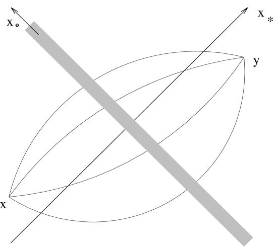
FIG. 13.: Quark propagator in the shock-wave field as a path integral.

We start the path-integral representation of a Green function in the external field:

$$\hbox{\bf\Big{(}$\!\!$\Big{(}}x\Big{|}\frac{1}{{\hbox{$\cal P$}\kern-3.40279pt\kern-2.5pt\hbox{$/$}\kern 3.40279pt\kern-2.5pt}}\Big{|}y\hbox{\bf\Big{)}$\!\!$\Big{)}}=-i\int_{0}^{\infty}\!d\tau\hbox{\bf\Big{(}$\!\!$\Big{(}}x\Big{|}{\cal P}e^{i\tau{\cal P}^{2}}\Big{|}y\hbox{\bf\Big{)}$\!\!$\Big{)}}=-i\int_{0}^{\infty}\!d\tau{\cal N}^{-1}\int_{x(0)=y}^{x(\tau)=x}\!{\cal D}x(t)\{{1\over 2}\not{\cdot x}+\not\!{B^{\Omega}}(x(\tau))\}e^{-i\int_{0}^{\tau}\!dt{\dot{x}^{2}\over 4}}$$ (A11)

$$Pexp\{ig\int_{0}^{\tau}\!dt(B^{\Omega}_{\mu}(x(t))\dot{x}^{\mu}(t)+{1\over 2}\sigma^{\mu\nu}G^{\Omega}_{\mu\nu}(x(t))\}$$ (A12)

where $\sigma_{\mu\nu}\equiv{i\over 2}(\gamma_{\mu}\gamma_{\nu}-\gamma_{\nu}\gamma_{\mu})$. First, it is easy to see that since in our external field (A9) the only nonzero components of the field tensor is $G^{\Omega}_{{}_{\circ}i_{\perp}}$ only the first two first term of the expansion of the exponent $\exp\{\int\!dt{i\over 2}(\sigma G^{\Omega})\}$ in powers of $(\sigma G)$ survive. Indeed, $\sigma^{\mu\nu}G^{\Omega}_{\mu\nu}={4i\over s_{0}}{\hbox{$p$}\kern-2.51563pt\kern-2.5pt\hbox{$/$}\kern 2.51563pt\kern-2.5pt}^{0}_{2}\gamma^{i}G^{\Omega}_{{}_{\circ}i}$ and therefore $(\sigma G^{\Omega})^{2}\sim({\hbox{$p$}\kern-2.51563pt\kern-2.5pt\hbox{$/$}\kern 2.51563pt\kern-2.5pt}_{2}\gamma^{i})^{2}=0$ since ${\hbox{$p$}\kern-2.51563pt\kern-2.5pt\hbox{$/$}\kern 2.51563pt\kern-2.5pt}_{2}$ commutes with $\gamma^{i}_{\perp}$. So, the phase factor for the motion of the particle in the external field (A9) has the form

$$Pe^{ig\int_{0}^{\tau}\!dtB^{\Omega}_{\mu}(x(t))\dot{x}_{\mu}(t)}+{2\gamma^{i}{\hbox{$p$}\kern-2.51563pt\kern-2.5pt\hbox{$/$}\kern 2.51563pt\kern-2.5pt}_{2}\over s}\int_{0}^{\tau}\!dt^{\prime}Pe^{ig\int_{t^{\prime}}^{\tau}\!dtB^{\Omega}_{\mu}(x(t))\dot{x}_{\mu}(t)}gG^{\Omega}_{{}_{\circ}i}(x(t^{\prime}))Pe^{ig\int^{t^{\prime}}_{0}\!dtB^{\Omega}_{\mu}(x(t))\dot{x}_{\mu}(t)}$$ (A13)

Let us consider the case $x_{\ast}>0,y_{\ast}<0$ as shown in Fig.13. Since the external field exists only within the infinitely thin wall at $x_{\ast}=0$ we can replace the gauge factor along the actual path $x_{\mu}(t)$ by the gauge factor along the straight-line path shown in Fig. 13 which intersects the plane $x_{\ast}=0$ at the same point $(z_{\circ},z_{\perp})$ at which the original path does. Since the shock-wave field outside the wall vanishes we may extend formally the limits of this segment to infinity and write the corresponding gauge factor as $U^{\Omega}(z_{\perp})=[-\infty p_{1}+z_{\perp},\infty p_{1}+z_{\perp}]$ where label ^Ω reminds that we calculate this eikonal factor in the field $B^{\Omega}$. The error brought by replacement of the original path $inside$ the wall by the segment of straight line parallel to $p_{1}$ is ${1\over\sqrt{\lambda}}$. Indeed, the time of the transition of the quark through the wall is proportional to the thickness of the wall which is $\sim{1\over\lambda}$ which means that it can deviate in the perpendicular directions iside the wall only to the distances $\sim{1\over\sqrt{\lambda}}$. Thus, if the quark intersects this wall at some point $(z_{\ast},z_{\perp})$ at the time $\tau^{\prime}$ the gauge factor (A14) reduces to:

$$U^{\Omega}(z_{\perp})+{\gamma^{i}\!{\hbox{$p$}\kern-2.51563pt\kern-2.5pt\hbox{$/$}\kern 2.51563pt\kern-2.5pt}_{2}\over\dot{x}_{\ast}(\tau^{\prime})}i\partial_{i}U^{\Omega}(z_{\perp})$$ (A14)

where the last term was obtained using the identity

$$\frac{\partial}{\partial x_{i}}U(x_{\perp})$$ (A15)

$$= -{2i\over s_{0}}\int\!dx_{\ast}[\infty p^{(0)}_{1}+x_{\perp},{2\over s_{0}}x_{*}p^{(0)}_{1}+x_{\perp}]G_{{}_{\circ}i}({2\over s_{0}}x_{*}p^{(0)}_{1}+x_{\perp})[{2\over s_{0}}x_{*}p^{(0)}_{1}+x_{\perp},-\infty p^{(0)}_{1}+x_{\perp}]$$ (A16)

and the factor $\dot{x}_{\ast}(\tau^{\prime})$ in eq. (A13) comes from changing of variable of integration from $t$ to $x_{\ast}(t)$. Similarly, the phase factor for the term in the r.h.s. of eq.(A12) which contains $\not\!B^{\Omega}(x(\tau))={2\over s_{0}}{\hbox{$p$}\kern-2.51563pt\kern-2.5pt\hbox{$/$}\kern 2.51563pt\kern-2.5pt}_{2}B^{\Omega}_{\circ}(x(\tau))$ in front of the gauge factor eq.(A12) can be reduced to

$$-{\hbox{$p$}\kern-2.51563pt\kern-2.5pt\hbox{$/$}\kern 2.51563pt\kern-2.5pt}_{2}{\partial\over\partial x_{*}}[{2\over s_{0}}x_{*}p^{(0)}_{1}+x_{\perp},-\infty+x_{\perp}]=-{\hbox{$p$}\kern-2.51563pt\kern-2.5pt\hbox{$/$}\kern 2.51563pt\kern-2.5pt}_{2}\delta(x_{*})[U(x_{\perp})-1]$$ (A17)

(The factor $\sim(\sigma G)$ is absent since it contains extra ${\hbox{$p$}\kern-2.51563pt\kern-2.5pt\hbox{$/$}\kern 2.51563pt\kern-2.5pt}_{2}$ and ${\hbox{$p$}\kern-2.51563pt\kern-2.5pt\hbox{$/$}\kern 2.51563pt\kern-2.5pt}_{2}^{2}=0$). If we now insert the expression for the phase factors (A13,A17) into the path integral (A12) we obtain

$$-{\hbox{$p$}\kern-2.51563pt\kern-2.5pt\hbox{$/$}\kern 2.51563pt\kern-2.5pt}_{2}\delta(x_{*})[U^{\Omega}(x_{\perp})-1]\int_{0}^{\infty}\!d\tau{\cal N}^{-1}\int^{x(\tau)=x}_{x(0)=y}\!{\cal D}x(t)e^{-i\int_{\tau}^{0}\!dt{\dot{x}^{2}\over 4}}-$$ (A18)

$${i\over 2}\int_{0}^{\infty}\!d\tau\int_{0}^{\tau}\!d\tau^{\prime}\int\!dz\delta(z_{*}){\cal N}^{-1}\int_{x(\tau^{\prime})=z}^{x(\tau)=x}\!{\cal D}x(t)\!\not{\dot{x}}(\tau)$$ (A19)

$$e^{-i\int_{\tau^{\prime}}^{\tau}\!dt{\dot{x}^{2}\over 4}}\{U^{\Omega}(z_{\perp})+{i\over\dot{x}_{*}(\tau^{\prime})}\not{\partial}U^{\Omega}(z_{\perp}){\hbox{$p$}\kern-2.51563pt\kern-2.5pt\hbox{$/$}\kern 2.51563pt\kern-2.5pt}_{2}\}{\cal N}^{-1}\int_{x(0)=y}^{x(\tau^{\prime})=z}\!{\cal D}x(t)\dot{x}_{*}(\tau^{\prime})e^{-i\int_{\tau^{\prime}}^{\tau}\!dt{\dot{x}^{2}\over 4}}$$ (A20)

The additional Jacobian factor $\dot{x}_{\ast}(\tau^{\prime})$ in the numerator in the second term in r.h.s. of this eq. comes due to the fact that we must integrate over all $\tau^{\prime}$ from $0$ to $\tau$ and therefore we insert $1=\int\!d\tau^{\prime}\dot{x}_{\ast}(\tau^{\prime})\delta(x_{\ast}(\tau^{\prime})-z_{\ast}))$ in the functional integral (A12). It is convenient to make a shift of time variable $\tau^{\prime}$ and to rewrite the eq.(A17) in the following way:

$$-{\hbox{$p$}\kern-2.51563pt\kern-2.5pt\hbox{$/$}\kern 2.51563pt\kern-2.5pt}_{2}\delta(x_{\ast})[U^{\Omega}(x_{\perp})-1]\int_{0}^{\infty}\!d\tau{\cal N}^{-1}\int^{x(\tau)=x}_{x(0)=y}\!{\cal D}x(t)\!\not{\dot{x}}(\tau)e^{-i\int_{\tau}^{0}\!dt{\dot{x}^{2}\over 4}}$$ (A21)

$$-{i\over 2}\int_{0}^{\infty}\!d\tau\int_{0}^{\infty}\!d\tau^{\prime}\int\!dz\delta(z_{\ast}){\cal N}^{-1}\int_{x(0)=z}^{x(\tau)=x}\!{\cal D}x(t)\!\not{\dot{x}}(\tau)e^{-i\int_{0}^{\tau}\!dt{\dot{x}^{2}\over 4}}{\cal N}^{-1}\int_{x(0)=y}^{x(\tau^{\prime})=z}\!{\cal D}x(t)$$ (A22)

$$\{\dot{x}_{\ast}(\tau^{\prime})U^{\Omega}(z_{\perp})+i\!\not{\partial_{i}}U^{\Omega}(z_{\perp})\!{\hbox{$p$}\kern-2.51563pt\kern-2.5pt\hbox{$/$}\kern 2.51563pt\kern-2.5pt}_{2}\}e^{-i\int_{\tau^{\prime}}^{\tau}\!dt{\dot{x}^{2}\over 4}}$$ (A23)

Now, using the path-integral representations for bare propagators:

$$\int_{0}^{\infty}\!d\tau{\cal N}^{-1}\int^{x(\tau)=x}_{x(0)=y}\!{\cal D}x(t)(\tau)e^{-i\int^{\tau}_{0}\!dt{\dot{x}^{2}\over 4}}=-\frac{1}{4\pi^{2}(x-y)^{2}}$$ (A24)

and

$$\int_{0}^{\infty}\!d\tau{\cal N}^{-1}\int^{x(\tau)=x}_{x(0)=y}\!{\cal D}x(t)\dot{x}_{\mu}(\tau)e^{-i\int^{\tau}_{0}\!dt{\dot{x}^{2}\over 4}}=\frac{i(x-y)_{\mu}}{\pi^{2}(x-y)^{4}}$$ (A25)

it is easy to see that the path-integral expression for the quark propagator in the shock-wave field (A24) reduces to

$$\hbox{\bf\Big{(}$\!\!$\Big{(}}x\Big{|}\frac{1}{{\hbox{$\cal P$}\kern-3.40279pt\kern-2.5pt\hbox{$/$}\kern 3.40279pt\kern-2.5pt}}\Big{|}y\hbox{\bf\Big{)}$\!\!$\Big{)}}$$ (A26)

$$= \frac{{\hbox{$p$}\kern-2.51563pt\kern-2.5pt\hbox{$/$}\kern 2.51563pt\kern-2.5pt}_{2}}{4\pi^{2}(x-y)^{2}}\delta(x_{\ast})[U^{\Omega}-1](x_{\perp})+\int\!dz\delta(z_{\ast})\frac{({\hbox{$x$}\kern-2.85764pt\kern-2.5pt\hbox{$/$}\kern 2.85764pt\kern-2.5pt}-{\hbox{$z$}\kern-2.54515pt\kern-2.5pt\hbox{$/$}\kern 2.54515pt\kern-2.5pt}){\hbox{$p$}\kern-2.51563pt\kern-2.5pt\hbox{$/$}\kern 2.51563pt\kern-2.5pt}_{2}}{2\pi^{2}(x-z)^{4}}\{U^{\Omega}(z_{\perp})\frac{-2iy_{\ast}}{2\pi^{2}(z-y)^{4}}$$ (A27)

$$- i\!\not{\partial}_{\perp}U^{\Omega}(z_{\perp})\frac{{\hbox{$p$}\kern-2.51563pt\kern-2.5pt\hbox{$/$}\kern 2.51563pt\kern-2.5pt}_{2}}{4\pi^{2}(z-y)^{2}}\}=i\int\!dz\delta(z_{\ast})\frac{({\hbox{$x$}\kern-2.85764pt\kern-2.5pt\hbox{$/$}\kern 2.85764pt\kern-2.5pt}-{\hbox{$z$}\kern-2.54515pt\kern-2.5pt\hbox{$/$}\kern 2.54515pt\kern-2.5pt}){\hbox{$p$}\kern-2.51563pt\kern-2.5pt\hbox{$/$}\kern 2.51563pt\kern-2.5pt}_{2}}{2\pi^{2}(x-z)^{4}}U^{\Omega}(z_{\perp})\frac{{\hbox{$z$}\kern-2.54515pt\kern-2.5pt\hbox{$/$}\kern 2.54515pt\kern-2.5pt}-{\hbox{$y$}\kern-2.6308pt\kern-2.5pt\hbox{$/$}\kern 2.6308pt\kern-2.5pt}}{2\pi^{2}(z-y)^{4}}$$ (A28)

(in the region $x_{\ast}>0,y_{\ast}<0$). It can be demonstrated that the answer for the propagator in the region $x_{\ast}<0,y_{\ast}>0$ differs from eq. (A28) by the substitution $U^{\Omega}\leftrightarrow U^{\Omega\dagger}$. Also, the propagator outside the shock-wave wall (at $x_{\ast},y_{\ast}<0$ or $x_{\ast},y_{\ast}>0$) coinside with bare propagator so the final answer for the quark Green function in the $B^{\Omega}$ background can be written down as:

$$\hbox{\bf\Big{(}$\!\!$\Big{(}}x\Big{|}\frac{1}{{\hbox{$\cal P$}\kern-3.40279pt\kern-2.5pt\hbox{$/$}\kern 3.40279pt\kern-2.5pt}}\Big{|}y\hbox{\bf\Big{)}$\!\!$\Big{)}}=$$ (A31)

$$-\frac{{\hbox{$x$}\kern-2.85764pt\kern-2.5pt\hbox{$/$}\kern 2.85764pt\kern-2.5pt}-{\hbox{$y$}\kern-2.6308pt\kern-2.5pt\hbox{$/$}\kern 2.6308pt\kern-2.5pt}}{2\pi^{2}(x-y)^{4}}+i\int\!dz\delta(z_{\ast})\frac{({\hbox{$x$}\kern-2.85764pt\kern-2.5pt\hbox{$/$}\kern 2.85764pt\kern-2.5pt}-{\hbox{$z$}\kern-2.54515pt\kern-2.5pt\hbox{$/$}\kern 2.54515pt\kern-2.5pt}){\hbox{$p$}\kern-2.51563pt\kern-2.5pt\hbox{$/$}\kern 2.51563pt\kern-2.5pt}_{2}}{2\pi^{2}(x-z)^{4}}\{[U^{\Omega}-1](z_{\perp})\Theta(x_{\ast})\Theta(-y_{\ast})-$$

$$[U^{\Omega\dagger}-1](z_{\perp})\Theta(y_{\ast})\Theta(-x_{\ast})\}\frac{{\hbox{$z$}\kern-2.54515pt\kern-2.5pt\hbox{$/$}\kern 2.54515pt\kern-2.5pt}-{\hbox{$y$}\kern-2.6308pt\kern-2.5pt\hbox{$/$}\kern 2.6308pt\kern-2.5pt}}{2\pi^{2}(z-y)^{4}}$$

where we have used the formula

$$i\int\!dz\delta(z_{\ast})\frac{{\hbox{$x$}\kern-2.85764pt\kern-2.5pt\hbox{$/$}\kern 2.85764pt\kern-2.5pt}-{\hbox{$z$}\kern-2.54515pt\kern-2.5pt\hbox{$/$}\kern 2.54515pt\kern-2.5pt}}{2\pi^{2}(x-z)^{4}}{\hbox{$p$}\kern-2.51563pt\kern-2.5pt\hbox{$/$}\kern 2.51563pt\kern-2.5pt}_{2}\frac{{\hbox{$z$}\kern-2.54515pt\kern-2.5pt\hbox{$/$}\kern 2.54515pt\kern-2.5pt}-{\hbox{$y$}\kern-2.6308pt\kern-2.5pt\hbox{$/$}\kern 2.6308pt\kern-2.5pt}}{2\pi^{2}(z-y)^{4}}=-\frac{{\hbox{$x$}\kern-2.85764pt\kern-2.5pt\hbox{$/$}\kern 2.85764pt\kern-2.5pt}-{\hbox{$y$}\kern-2.6308pt\kern-2.5pt\hbox{$/$}\kern 2.6308pt\kern-2.5pt}}{2\pi^{2}(x-y)^{4}}(\Theta(x_{\ast})-\Theta(y_{\ast}))$$ (A32)

to separate the bare propagator. In the momentum representation this answer (A31) takes the form:

$$\hbox{\bf\Big{(}$\!\!$\Big{(}}k\Big{|}\frac{1}{{\hbox{$\cal P$}\kern-3.40279pt\kern-2.5pt\hbox{$/$}\kern 3.40279pt\kern-2.5pt}}\Big{|}k-p\hbox{\bf\Big{)}$\!\!$\Big{)}}$$ (A33)

$$= (2\pi)^{4}\delta^{(4)}(p)\frac{\alpha^{0}_{k}{\hbox{$p$}\kern-2.51563pt\kern-2.5pt\hbox{$/$}\kern 2.51563pt\kern-2.5pt}^{0}_{1}+\beta_{k}{\hbox{$p$}\kern-2.51563pt\kern-2.5pt\hbox{$/$}\kern 2.51563pt\kern-2.5pt}_{2}+{\hbox{$k$}\kern-2.76042pt\kern-2.5pt\hbox{$/$}\kern 2.76042pt\kern-2.5pt}_{\perp}}{\alpha^{0}_{k}\beta_{k}s_{0}-k_{\perp}^{2}+\mbox{$i\epsilon$}}~{}+$$ (A36)

$$2\pi i\delta(\alpha_{p})\frac{(\alpha_{k}{\hbox{$p$}\kern-2.51563pt\kern-2.5pt\hbox{$/$}\kern 2.51563pt\kern-2.5pt}^{0}_{1}+{\hbox{$k$}\kern-2.76042pt\kern-2.5pt\hbox{$/$}\kern 2.76042pt\kern-2.5pt}_{\perp})p_{2}}{\alpha^{0}_{k}\beta_{k}s_{0}-k_{\perp}^{2}+\mbox{$i\epsilon$}}{2\over s_{0}}[\Theta(\alpha^{0}_{k})(U^{\Omega}(p_{\perp})-4\pi^{2}\delta(p_{\perp}))-$$

$$\Theta(-\alpha^{0}_{k})(U^{\Omega\dagger}(p)-4\pi^{2}\delta(p_{\perp}))]\frac{\alpha^{0}_{k}{\hbox{$p$}\kern-2.51563pt\kern-2.5pt\hbox{$/$}\kern 2.51563pt\kern-2.5pt}^{0}_{1}+({\hbox{$k$}\kern-2.76042pt\kern-2.5pt\hbox{$/$}\kern 2.76042pt\kern-2.5pt}-{\hbox{$p$}\kern-2.51563pt\kern-2.5pt\hbox{$/$}\kern 2.51563pt\kern-2.5pt})_{\perp}}{\alpha^{0}_{k}(\beta_{k}-\beta_{p})s_{0}-(k-p)_{\perp}^{2}+\mbox{$i\epsilon$}}$$

which agrees with eq.(58) after integration over $\alpha^{0}_{p}$ and rescaling $\alpha_{p}={1\over\lambda}\alpha^{0}_{p}$ (here $\alpha^{0}$ is the Sudakov component along vector $p^{0}_{1}$).

Now, one easily obtains the quark propagator in the original field $B_{\mu}$ eq. (A4) by making back the gauge rotation of the answer (A31) with matrix $\Omega^{-1}$. It is convenient to represent the result in the following form:

$$\hbox{\bf\Big{(}$\!\!$\Big{(}}x\Big{|}\frac{1}{{\hbox{$\cal P$}\kern-3.40279pt\kern-2.5pt\hbox{$/$}\kern 3.40279pt\kern-2.5pt}}\Big{|}y\hbox{\bf\Big{)}$\!\!$\Big{)}}~{}=$$ (A37)

$$- \frac{{\hbox{$x$}\kern-2.85764pt\kern-2.5pt\hbox{$/$}\kern 2.85764pt\kern-2.5pt}-{\hbox{$y$}\kern-2.6308pt\kern-2.5pt\hbox{$/$}\kern 2.6308pt\kern-2.5pt}}{2\pi^{2}(x-y)^{4}}[x,y]\Theta(x_{\ast}y_{\ast})$$ (A38)

$$+ i\int\!dz\delta(z_{\ast})\frac{{\hbox{$x$}\kern-2.85764pt\kern-2.5pt\hbox{$/$}\kern 2.85764pt\kern-2.5pt}-{\hbox{$z$}\kern-2.54515pt\kern-2.5pt\hbox{$/$}\kern 2.54515pt\kern-2.5pt}}{2\pi^{2}(x-z)^{4}}\{U(z_{\perp};x,y)\Theta(x_{\ast})\Theta(-y_{\ast})-U^{\dagger}(z_{\perp};x,y)\Theta(y_{\ast})\Theta(-x_{\ast})\}\frac{{\hbox{$z$}\kern-2.54515pt\kern-2.5pt\hbox{$/$}\kern 2.54515pt\kern-2.5pt}-{\hbox{$y$}\kern-2.6308pt\kern-2.5pt\hbox{$/$}\kern 2.6308pt\kern-2.5pt}}{2\pi^{2}(z-y)^{4}}$$ (A39)

where

$$U(z_{\perp};x,y)=[x,z_{x}][z_{x},z_{y}][z_{y},y]~{}~{},{}~{}~{}z_{x}\equiv({2\over s_{0}}z_{\circ}p^{(0)}_{1}+{2\over s_{0}}x_{\ast}p_{2},z_{\perp}),~{}~{}z_{y}=z_{x}(x_{\ast}\leftrightarrow y_{\ast})$$ (A40)

is a gauge factor for the contour made from segments of straight lines as shown in Fig. 14. (Since the field $B_{\mu}$ outside the shock-wave wall is a pure gauge the precise form of the contour does not matter as long as it starts at the point $x$, intersects the wall at the point $z$ in the direction collinear to $p_{2}$ and ends at the point $y$).

For the quark-antiquark amplitude in the shock-wave field (see Fig 14)

                 

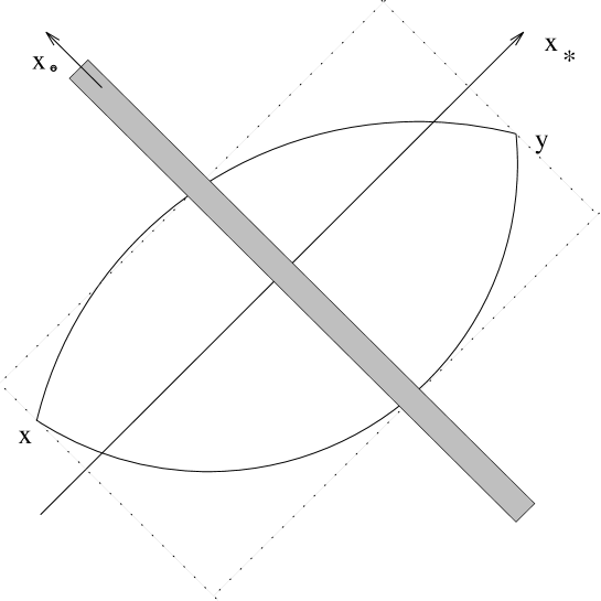
FIG. 14.: Quark-antiquark propagation in the shock wave.

we get

$$\mathop{\rm Tr}\gamma_{\mu}\hbox{\bf\Big{(}$\!\!$\Big{(}}x\Big{|}\frac{1}{{\hbox{$\cal P$}\kern-3.40279pt\kern-2.5pt\hbox{$/$}\kern 3.40279pt\kern-2.5pt}}\Big{|}y\hbox{\bf\Big{)}$\!\!$\Big{)}}\gamma_{\nu}\hbox{\bf\Big{(}$\!\!$\Big{(}}y\Big{|}\frac{1}{{\hbox{$\cal P$}\kern-3.40279pt\kern-2.5pt\hbox{$/$}\kern 3.40279pt\kern-2.5pt}}\Big{|}x\hbox{\bf\Big{)}$\!\!$\Big{)}}=$$ (A43)

$$\frac{Tr\gamma_{\mu}({\hbox{$x$}\kern-2.85764pt\kern-2.5pt\hbox{$/$}\kern 2.85764pt\kern-2.5pt}-{\hbox{$y$}\kern-2.6308pt\kern-2.5pt\hbox{$/$}\kern 2.6308pt\kern-2.5pt})\gamma_{\nu}({\hbox{$y$}\kern-2.6308pt\kern-2.5pt\hbox{$/$}\kern 2.6308pt\kern-2.5pt}-{\hbox{$x$}\kern-2.85764pt\kern-2.5pt\hbox{$/$}\kern 2.85764pt\kern-2.5pt})}{4\pi^{4}(x-y)^{8}}\Theta(x_{\ast}y_{\ast})-$$

$$\Theta(-x_{\ast}y_{\ast})\int\!dz\delta(z_{\ast})\int\!dz^{\prime}\delta(z^{\prime}_{\ast})Tr\gamma_{\mu}\frac{{\hbox{$x$}\kern-2.85764pt\kern-2.5pt\hbox{$/$}\kern 2.85764pt\kern-2.5pt}-{\hbox{$z$}\kern-2.54515pt\kern-2.5pt\hbox{$/$}\kern 2.54515pt\kern-2.5pt}}{2\pi^{2}(x-z)^{4}}{\hbox{$p$}\kern-2.51563pt\kern-2.5pt\hbox{$/$}\kern 2.51563pt\kern-2.5pt}_{2}\frac{{\hbox{$z$}\kern-2.54515pt\kern-2.5pt\hbox{$/$}\kern 2.54515pt\kern-2.5pt}-{\hbox{$y$}\kern-2.6308pt\kern-2.5pt\hbox{$/$}\kern 2.6308pt\kern-2.5pt}}{2\pi^{2}(z-y)^{4}}\gamma_{\nu}\frac{{\hbox{$y$}\kern-2.6308pt\kern-2.5pt\hbox{$/$}\kern 2.6308pt\kern-2.5pt}-{\hbox{$z$}\kern-2.54515pt\kern-2.5pt\hbox{$/$}\kern 2.54515pt\kern-2.5pt}^{\prime}}{2\pi^{2}(y-z^{\prime})^{4}}{\hbox{$p$}\kern-2.51563pt\kern-2.5pt\hbox{$/$}\kern 2.51563pt\kern-2.5pt}_{2}\frac{{\hbox{$z$}\kern-2.54515pt\kern-2.5pt\hbox{$/$}\kern 2.54515pt\kern-2.5pt}^{\prime}-{\hbox{$x$}\kern-2.85764pt\kern-2.5pt\hbox{$/$}\kern 2.85764pt\kern-2.5pt}}{2\pi^{2}(z^{\prime}-x)^{4}}W(z_{\perp};z^{\prime}_{\perp})$$

where we can write down the gauge factor $W(z_{\perp};z^{\prime}_{\perp})\equiv U(z_{\perp};x,y)U^{\dagger}(z^{\prime}_{\perp};y,x)$ as a product of two infinite Wilson-lines operators connected by gauge segments at $\pm\infty$:

$$W(z_{\perp};z^{\prime}_{\perp})$$ (A44)

$$= \lim_{u\rightarrow\infty}[-up_{1}+z_{\perp},up_{1}+z_{\perp}][up_{1}+z_{\perp},up_{1}+z^{\prime}_{\perp}][up_{1}+z^{\prime}_{\perp},-up_{1}+z^{\prime}_{\perp}][-up_{1}+z^{\prime}_{\perp},-up_{1}+z_{\perp}]$$ (A45)

The precise form of the connecting contour does not matter as long as it is outside the shock wave. We have chosen this contour in such a way that the gauge factor (A45) is the same for the field $B_{\mu}$ and for the original field $A_{\mu}$ (see eq. (A4). Now, substituting our result for quark-antiquark propagation (A43) in the r.h.s of eq. (A1) one recovers after some algebra the eqs. (67, 70) for the impact factor.

B One-loop evolution: Wilson lines in a shock-wave background.

Let us now find how the one-loop evolution of Wilson-line operators can be obtained using the shock-wave picture of high-energy scattering. To this end, consider the near-light-like operators ${\hat{U}^{\zeta}}$ and $\hat{U}^{\dagger\zeta}$ in the external field. Making the rescaling (A4) we obtain:

$$\langle[\infty p_{A}+x_{\perp},-\infty p_{A}+y_{\perp}][-\infty p_{A}+x_{\perp},\infty p_{A}+y_{\perp}]\rangle_{A}=$$ (B1)

$$\langle[\infty p^{(0)}_{A}+x_{\perp},-\infty p^{(0)}_{A}+y_{\perp}][-\infty p^{(0)}_{A}+x_{\perp},\infty p^{(0)}_{A}+y_{\perp}]\rangle_{B}$$ (B2)

where the shock-wave field is given by formulas (A4-A9) We must find the derivative $\zeta{\partial\over\partial\zeta}$ given by eq. (131). After rescaling according to eq. (131) one obtains:

$$\zeta{\partial\over\partial\zeta}\langle\hat{U}(x_{\perp})\hat{U}^{\dagger}(y_{\perp})\rangle_{A}$$ (B3)

$$= ig{p_{A}^{2}\over s_{0}}\int\!udu\langle[\infty p^{(0)}_{A}+x_{\perp},up^{(0)}_{A}+x_{\perp}]\hat{F}_{\ast\circ}(up^{(0)}_{A}+x_{\perp})[up^{(0)}_{A}+x_{\perp},-\infty p^{(0)}_{A}+x_{\perp}]\hat{U}^{\dagger}(y_{\perp})\rangle_{B}-$$ (B5)

$$ig{p_{A}^{2}\over s_{0}}\int\!udu\langle\hat{U}(x_{\perp})[-\infty p^{(0)}_{A}+y_{\perp},up^{(0)}_{A}+y_{\perp}]\hat{F}_{\ast\circ}(up^{(0)}_{A}+y_{\perp})[up^{(0)}_{A}+y_{\perp},\infty p^{(0)}_{A}+y_{\perp}]\rangle_{B}$$

Since the (_∗∘) component of the field strength tensor vanishes for the shock-wave field (A9) the only nonzero contribution comes from the diagrams with quantum gluons. In the lowest nontrivial order in $\alpha_{s}$ there are three diargams shown in Fig. 15.

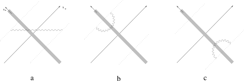
FIG. 15.: Path integrals describing one-loop diagrams for Wilson-line operators in the shock-wave field background.

Consider at first the diagram shown in Fig. 15a (which corresponds to the case $x_{\ast}>0$, $y_{\ast}<0$). The corresponding contribution to r.h.s. of eq. (B5) is:

$$-g^{2}\int du[\infty p^{(0)}_{A}+x_{\perp},up^{(0)}_{A}+x_{\perp}]t^{a}[up^{(0)}_{A}+x_{\perp},-\infty p^{(0)}_{A}+x_{\perp}]$$ (B6)

$$\otimes\int dv[-\infty p^{(0)}_{A}+y_{\perp},vp^{(0)}_{A}+y_{\perp}]t^{b}[vp^{(0)}_{A}+y_{\perp},\infty p^{(0)}_{A}+y_{\perp}]$$ (B7)

$$\hbox{\bf\Big{(}$\!\!$\Big{(}}up^{(0)}_{A}+x_{\perp}\Big{|}up_{\ast}\{(p^{(0)}_{A\xi}-{\cal P}_{\circ}\frac{p_{2\xi}}{p\cdot p_{2}})[\frac{1}{{\cal P}^{2}g_{\xi\eta}+2iG_{\xi\eta}}-\frac{1}{{\cal P}^{2}g_{\xi\lambda}+2iG_{\xi\lambda}}(D^{\alpha}G_{\alpha\lambda}\frac{p_{2\rho}}{p\cdot p_{2}}+\frac{p_{2\lambda}}{p\cdot p_{2}}D^{\alpha}G_{\alpha\rho}-$$ (B8)

$$\frac{p_{2\lambda}}{p\cdot p_{2}}{\cal P}^{\beta}D^{\alpha}G_{\alpha\beta}\frac{p_{2\rho}}{p\cdot p_{2}})\frac{1}{{\cal P}^{2}g_{\rho\eta}+2iF_{\rho\eta}}+...](p^{(0)}_{A\eta}-\frac{p_{2\eta}}{p\cdot p_{2}}{\cal P}_{\circ})\}-v\left\{...\right\}p_{\ast}\Big{|}vp^{(0)}_{A}+y_{\perp}\hbox{\bf\Big{)}$\!\!$\Big{)}}_{ab}$$ (B9)

As we discussed in Sect.4 terms in parentheses proportional to ${\cal P}_{\circ}$ vanish after integration by parts (cf. eq. (147)). Further, it is easy to check that since the only nonzero component of field strength tensor for the shock wave is $G^{\Omega}_{\circ\perp}$ the expression in braces in eq. (B9) can be reduced to ${\cal O}^{\Omega}_{\circ\circ}$ where the operator ${\cal O}^{\Omega}_{\mu\nu}$ is given by eq. (157). Starting from this point it is convenient to perform the calculation in the background of the rotated field $B^{\Omega}$ (A10) which is $0$ everywhere except the shock-wave wall. (We shall make the rotation back to field $B$ in the final answer). Then the gauge factors $[\infty,u]t^{a}[u,-\infty]$ and $[\infty,v]t^{b}[v,-\infty]$ in eq. (B9) reduce to $t^{a}[\infty,-\infty]\otimes t^{b}[-\infty,\infty]$ (at $x_{\ast}>0,y_{\ast}<0$) and we obtain:

$$-g^{2}t^{a}U^{\Omega}\otimes t^{b}U^{\dagger\Omega}\int\!du\int\!dv(u-v)\hbox{\bf\Big{(}$\!\!$\Big{(}}up^{(0)}_{A}+x_{\perp}\Big{|}p_{\ast}{\cal O}^{\Omega}_{\circ\circ}\Big{|}vp^{(0)}_{A}+y_{\perp}\hbox{\bf\Big{)}$\!\!$\Big{)}}_{ab}$$ (B10)

where we have used the fact that the operator $p_{\ast}$ commutes with ${\cal O}^{\Omega}$. Let us now derive the formula for the $(_{\circ\circ})$ component of the gluon propagator $(x|{\cal O}^{\Omega}|y)$ in the shock-wave background. The path-integral representation of $(x|{\cal O}^{\Omega}_{\circ\circ}|y)$ has the form:

$$\hbox{\bf\Big{(}$\!\!$\Big{(}}x\Big{|}4\frac{1}{{\cal P}^{2}}G^{\xi\Omega}_{\circ}\frac{1}{{\cal P}^{2}}G^{\Omega}_{\xi\circ}\frac{1}{{\cal P}^{2}}-\frac{1}{{\cal P}^{2}}(D^{\alpha}G^{\Omega}_{\alpha\circ}\frac{s_{0}}{2p_{\ast}}+\frac{s_{0}}{2p_{\ast}}D^{\alpha}G^{\Omega}_{\alpha\nu}-\frac{s_{0}}{2p_{\ast}}{\cal P}^{\beta}D^{\alpha}G^{\Omega}_{\alpha\beta}\frac{s_{0}}{2p_{\ast}})\frac{1}{{\cal P}^{2}}\Big{|}y\hbox{\bf\Big{)}$\!\!$\Big{)}}$$ (B11)

$$= i\int_{0}^{\infty}\!d\tau\int_{0}^{\tau}\!d\tau^{\prime}\hbox{\bf\Big{(}$\!\!$\Big{(}}x\Big{|}e^{i(\tau-\tau^{\prime}){\cal P}^{2}}\{G^{\alpha\Omega}_{\circ}\int_{0}^{\tau^{\prime}}\!d\tau^{\prime\prime}e^{i(\tau^{\prime}-\tau^{\prime\prime}){\cal P}^{2}}\{G^{\Omega}_{\alpha\circ}e^{i\tau^{\prime\prime}{\cal P}^{2}}-{is_{0}\over 2p_{\ast}}D^{\alpha}G^{\Omega}_{\alpha\circ}e^{i\tau^{\prime\prime}{\cal P}^{2}}\}\Big{|}y\hbox{\bf\Big{)}$\!\!$\Big{)}}$$ (B12)

$$= i\int_{0}^{\infty}\!d\tau{\cal N}^{-1}\int_{x(0)=y}^{x(\tau)=x}\!{\cal D}x(t)e^{-i\int_{0}^{\tau}\!dt{\dot{x}^{2}\over 4}}\{4\int_{0}^{\tau}\!d\tau^{\prime}\int_{0}^{\tau^{\prime}}\!d\tau^{\prime\prime}Pe^{ig\int_{\tau^{\prime}}^{\tau}\!dtB^{\Omega}_{\mu}(x(t))\dot{x}_{\mu}(t)}gG^{\Omega}_{{}_{\circ}i}(x(\tau^{\prime}))$$ (B15)

$$Pe^{ig\int^{\tau^{\prime}}_{\tau^{\prime\prime}}\!dtB^{\Omega}_{\mu}(x(t))\dot{x}_{\mu}(t)}\int_{0}^{\tau^{\prime}}\!d\tau^{\prime\prime}Pe^{ig\int_{\tau^{\prime\prime}}^{\tau^{\prime}}\!dtB^{\Omega}_{\mu}(x(t))\dot{x}_{\mu}(t)}gG^{\Omega}_{{}_{\circ}i}(x(\tau^{\prime\prime}))Pe^{ig\int^{\tau^{\prime\prime}}_{0}\!dtB^{\Omega}_{\mu}(x(t))\dot{x}_{\mu}(t)}$$

$$+i\int_{0}^{\tau}\!d\tau^{\prime}Pe^{ig\int_{\tau^{\prime}}^{\tau}\!dtB^{\Omega}_{\mu}(x(t))\dot{x}_{\mu}(t)}{s_{0}\over\dot{x_{\ast}}(\tau^{\prime})}gD^{\alpha}G^{\Omega}_{\alpha\circ}(x(\tau^{\prime}))Pe^{ig\int^{\tau^{\prime}}_{0}\!dtB^{\Omega}_{\mu}(x(t))\dot{x}_{\mu}(t)}\}$$

As we discussed above, the transition through the shock wave occurs in a short time $\sim{1\over\lambda}$ so the gluon has no time to deviate in the transverse directions and therefore the gauge factors in eq. (B15) can be approximated by segments of Wilson lines. One obtains then (cf. eq. (A23)):

$$\hbox{\bf\Big{(}$\!\!$\Big{(}}x\Big{|}{\cal O}^{\Omega}_{\circ\circ}\Big{|}y\hbox{\bf\Big{)}$\!\!$\Big{)}}$$ (B16)

$$= {i\over 2}s_{0}^{2}\int_{0}^{\infty}\!d\tau\int_{0}^{\tau}\!d\tau^{\prime}\int\!dz\delta(z_{*}){\cal N}^{-1}\int_{x(\tau^{\prime})=z}^{x(\tau)=x}\!{\cal D}x(t)\!e^{-i\int_{\tau^{\prime}}^{\tau}\!dt{\dot{x}^{2}\over 4}}$$ (B18)

$${1\over\dot{x}_{\ast}(\tau^{\prime})}\{2[GG]^{\Omega}(z_{\perp})-i[DG]^{\Omega}(z_{\perp})\}{\cal N}^{-1}\int_{x(0)=y}^{x(\tau^{\prime})=z}\!{\cal D}x(t)e^{-i\int_{\tau^{\prime}}^{\tau}\!dt{\dot{x}^{2}\over 4}}$$

where $[GG]^{\Omega}$ and $[DG]^{\Omega}$ are the notations for the gauge factors (167) calculated for the background field $B^{\Omega}_{\mu}$:

$$[DG]^{\Omega}(x_{\perp})= \int du[\infty p_{1}+x_{\perp},up_{1}+x_{\perp}]D^{\alpha}G^{\Omega}_{\alpha\circ}(up_{1}+x_{\perp})[up_{1}+x_{\perp},-\infty p_{1}+x_{\perp}]$$ (B19)

$$[GG]^{\Omega}(x_{\perp})= \int\!du\int\!dv\Theta(u-v)[\infty p_{1}+x_{\perp},up_{1}+x_{\perp}]G^{\xi\Omega}_{\circ}(up_{1}+x_{\perp})$$ (B21)

$$[up_{1}+x_{\perp},vp_{1}+x_{\perp}]G^{\Omega}_{\xi\circ}(vp_{1}+x_{\perp})[vp_{1}+x_{\perp},-\infty p_{1}+x_{\perp}]$$

As we noted in Sect.4 the gauge factor $-i[DG]+2[GG]$ in braces in eq. (B15) is in fact the total derivative of $U$ with respect to translations in the perpendicular directions so we get:

$$\hbox{\bf\Big{(}$\!\!$\Big{(}}x\Big{|}{\cal O}^{\Omega}_{\circ\circ}\Big{|}y\hbox{\bf\Big{)}$\!\!$\Big{)}}~{}=$$ (B23)

$${i\over 2}s_{0}^{2}\int_{0}^{\infty}\!d\tau\int_{0}^{\tau}\!d\tau^{\prime}\int\!dz\delta(z_{*}){\cal N}^{-1}\int_{x(\tau^{\prime})=z}^{x(\tau)=x}\!{\cal D}x(t)\!e^{-i\int_{\tau^{\prime}}^{\tau}\!dt{\dot{x}^{2}\over 4}}{1\over\dot{x}_{\ast}(\tau^{\prime})}\partial_{\perp}^{2}U^{\Omega}(x_{\perp}){\cal N}^{-1}\int_{x(0)=y}^{x(\tau^{\prime})=z}\!{\cal D}x(t)e^{-i\int_{\tau^{\prime}}^{\tau}\!dt{\dot{x}^{2}\over 4}}$$

Using now the path-integral representation for bare propagator (A24) and the following formula

$$\int_{0}^{\infty}\!d\tau{\cal N}^{-1}\int^{x(\tau)=x}_{x(0)=y}\!{\cal D}x(t){1\over\dot{x}_{\ast}(0)}e^{-i\int^{\tau}_{0}\!dt{\dot{x}^{2}\over 4}}=i\frac{\ln(x-y)^{2}}{16\pi^{2}(x-y)_{\ast}}$$ (B24)

we finally obtain the $(_{\circ\circ})$ component of the gluon propagator in the shock-wave background in the form:

$$\hbox{\bf\Big{(}$\!\!$\Big{(}}x\Big{|}{\cal O}^{\Omega}_{\circ\circ}\Big{|}y\hbox{\bf\Big{)}$\!\!$\Big{)}}$$ (B25)

$$= {s_{0}^{2}\over 2}\int\!dz\delta(z_{\ast})\frac{\ln(x-z)^{2}}{16\pi^{2}x_{\ast}}[\partial^{2}U^{\Omega}(z_{\perp})\Theta(x_{\ast})\Theta(-y_{\ast})-\partial^{2}U^{\dagger\Omega}(z_{\perp})\Theta(-x_{\ast})\Theta(y_{\ast})]\frac{1}{4\pi^{2}(z-y)^{2}}$$ (B26)

where we have added the similar term corresponding to the case $x_{\ast}<0,y_{\ast}>0$. We need also the ${\partial\over\partial x_{\circ}}$ derivative of this propagator (see eq. (B10) which is:

$$\hbox{\bf\Big{(}$\!\!$\Big{(}}x\Big{|}p_{\ast}{\cal O}^{\Omega}_{\circ\circ}\Big{|}y\hbox{\bf\Big{)}$\!\!$\Big{)}}={is_{0}^{2}\over 64\pi^{4}}\int\!dz\frac{\delta(z_{\ast})}{(x-y)^{2}}[\partial^{2}U^{\Omega}(z_{\perp})\Theta(x_{\ast})\Theta(-y_{\ast})-\partial^{2}U^{\dagger\Omega}(z_{\perp})\Theta(-x_{\ast})\Theta(y_{\ast})]\frac{1}{(z-y)^{2}}$$ (B27)

In the momentum representation this eq. takes the form:

$$\hbox{\bf\Big{(}$\!\!$\Big{(}}k\Big{|}{\cal O}^{\Omega}_{\circ\circ}\Big{|}k-p\hbox{\bf\Big{)}$\!\!$\Big{)}}_{ab}~{}=~{}$$ (B29)

$$\frac{-is_{0}}{2}2\pi\delta(\alpha^{0}_{p})\frac{1}{\alpha^{0}_{k}\beta_{k}s-k_{\perp}^{2}+\mbox{$i\epsilon$}}(\Theta(\alpha^{0}_{k})(\partial_{\perp}^{2}U^{\Omega}(p_{\perp}))-\Theta(-\alpha^{0}_{k})(\partial_{\perp}^{2}U^{\dagger\Omega}(p_{\perp}))\frac{1}{\alpha^{0}_{k}(\beta_{k}-\beta_{p})s-(k-p)_{\perp}^{2}+\mbox{$i\epsilon$}}$$

which agrees with eq. (162) after rescaling $\alpha_{p}={1\over\lambda}\alpha^{0}_{p}$. Substituting now the eq. (B27) into eq. (B10) one recovers eq. (167) after some algebra

$${g^{2}\over 4\pi}\hbox{\bf\Big{(}$\!\!$\Big{(}}x_{\perp}\Big{|}\frac{1}{p^{2}}\partial_{\perp}^{2}U^{\Omega}\frac{1}{p^{2}}\Big{|}y_{\perp}\hbox{\bf\Big{)}$\!\!$\Big{)}}_{ab}t^{a}U^{\Omega}(x_{\perp})\otimes t^{b}U^{\dagger\Omega}(y_{\perp})+$$ (B30)

$${g^{2}\over 4\pi}\hbox{\bf\Big{(}$\!\!$\Big{(}}x_{\perp}\Big{|}\frac{1}{p^{2}}\partial_{\perp}^{2}U^{\dagger\Omega}\frac{1}{p^{2}}\Big{|}y_{\perp}\hbox{\bf\Big{)}$\!\!$\Big{)}}_{ab}U^{\Omega}(x_{\perp})t^{a}\otimes U^{\dagger\Omega}(y_{\perp})t^{b}$$ (B31)

Let us consider now the diagram shown in Fig. 15b. The calculation is very similar to the case of Fig. 15a diagram considered above so we shall only briefly outline the calculation. One starts with the corresponding contribution to r.h.s.of eq. (B5) which has the form (cf. (B9):

(B32)

$$- g^{2}\zeta\int\!du\int\!dv\Theta(u-v)[\infty p^{(0)}_{A}+x_{\perp},up^{(0)}_{A}+x_{\perp}]t^{a}[up^{(0)}_{A}+x_{\perp},vp^{(0)}_{A}+x_{\perp}]$$ (B36)

$$t^{b}[vp^{(0)}_{A}+x_{\perp},-\infty p^{(0)}_{A}+x_{\perp}]\otimes U^{\dagger}(y_{\perp})$$

$$\hbox{\bf\Big{(}$\!\!$\Big{(}}up^{(0)}_{A}+x_{\perp}\Big{|}up_{\ast}\{(p^{(0)}_{A\xi}-{\cal P}_{\circ}\frac{p_{2\xi}}{p\cdot p_{2}})[\frac{1}{{\cal P}^{2}g_{\xi\eta}+2iG_{\xi\eta}}-\frac{1}{{\cal P}^{2}g_{\xi\lambda}+2iG^{\Omega}_{\xi\lambda}}(D^{\alpha}G^{\Omega}_{\alpha\lambda}\frac{p_{2\rho}}{p\cdot p_{2}}+\frac{p_{2\lambda}}{p\cdot p_{2}}D^{\alpha}G^{\Omega}_{\alpha\rho}-$$

$$\frac{p_{2\lambda}}{p\cdot p_{2}}{\cal P}^{\beta}D^{\alpha}G_{\alpha\beta}\frac{p_{2\rho}}{p\cdot p_{2}})\frac{1}{{\cal P}^{2}g_{\rho\eta}+2iG_{\rho\eta}}+...](p^{(0)}_{A\eta}-\frac{p_{2\eta}}{p\cdot p_{2}}{\cal P}_{\circ})\}-v\left\{...\right\}p_{\ast}\Big{|}vp^{(0)}_{A}+x_{\perp}\hbox{\bf\Big{)}$\!\!$\Big{)}}_{ab}$$

As we demonstrated in Sect.4 the terms in parentheses proportional to ${\cal P}_{\bullet}$ vanish and after that the operator in braces reduce to ${\cal O}_{\circ\circ}$. Again, it is convenient to make a gauge transformation to the rotated field (A10) which is 0 everywhere except the shock wave. Then the gauge factor $[\infty,u]t^{a}[u,v]t^{b}[v,-\infty]$ in eq. (B29) reduces to $t^{a}[\infty,-\infty]t^{b}$ (at $x_{\ast}>0,y_{\ast}<0$) and we obtain:

$$-g^{2}t^{a}U^{\Omega}t^{b}\otimes U^{\dagger\Omega}\int\!du\int\!dv(u-v)\hbox{\bf\Big{(}$\!\!$\Big{(}}up^{(0)}_{A}+x_{\perp}\Big{|}p_{\ast}{\cal O}^{\Omega}_{\circ\circ}\Big{|}vp^{(0)}_{A}+x_{\perp}\hbox{\bf\Big{)}$\!\!$\Big{)}}_{ab}$$ (B37)

Using the expression (B27) for the gluon propagator in the shock-wave background after some algebra one obtains the answer (202):

$$-{g^{2}\over 4\pi}t^{a}U^{\Omega}(x_{\perp})t^{b}\otimes U^{\dagger\Omega}(y_{\perp})\hbox{\bf\Big{(}$\!\!$\Big{(}}x_{\perp}\Big{|}\frac{1}{p^{2}}(\partial^{2}U^{\Omega})\frac{1}{p^{2}}\Big{|}x_{\perp}\hbox{\bf\Big{)}$\!\!$\Big{)}}_{ab}$$ (B38)

The contribution of the diagram in Fig. 15 differs from eq. (B38) only in change $U\leftrightarrow U^{\dagger},~{}x\leftrightarrow y$ (see eq. (A43)). Combining these expressions, one obtains the answer in the rotated field (A10) in the form:

$${g^{2}\over 16\pi^{3}}\int\!dz_{\perp}$$ (B43)

$$\left\{[\{U^{\dagger\Omega}(z_{\perp})U^{\Omega}(x_{\perp})\}^{k}_{j}\{U^{\Omega}(z_{\perp})U^{\dagger\Omega}(y_{\perp})\}^{i}_{l}+\{U^{\Omega}(x_{\perp})U^{\dagger\Omega}(z_{\perp})\}^{i}_{l}\{U^{\dagger\Omega}(y_{\perp})U^{\Omega}(z_{\perp})\}^{k}_{j}-\right.$$

$$\left.\delta^{k}_{j}\{U^{\Omega}(x_{\perp})U^{\dagger\Omega}(y_{\perp})\}^{i}_{l}-\delta^{i}_{l}\{U^{\dagger\Omega}(y_{\perp})U^{\Omega}(x_{\perp})\}^{k}_{j}]\frac{(x-z,y-z)_{\perp}}{(x-z)_{\perp}^{2}(y-z)_{\perp}^{2}}-\right.$$

$$\left.[\{U^{\Omega}(z_{\perp})\}^{i}_{j}\mathop{\rm Tr}\{U^{\Omega}(x_{\perp})U^{\dagger\Omega}(z_{\perp})\}-N_{c}\{U^{\Omega}(x_{\perp})\}^{i}_{j})U^{\dagger\Omega}(y_{\perp})^{k}_{l}\frac{1}{(x-z)_{\perp}^{2}}-\right.$$

$$\left.\{U^{\Omega}(x_{\perp})\}^{i}_{j}[U^{\dagger\Omega}(z_{\perp})^{k}_{l}\mathop{\rm Tr}\{U^{\Omega}(z_{\perp})U^{\dagger\Omega}(y_{\perp})\}-N_{c}\{U^{\dagger\Omega}(y_{\perp})\}^{k}_{l})]\frac{1}{(y-z)_{\perp}^{2}}\right\}$$

Now we must perform the gauge rotation back to the ”original” field $B_{\mu}$. The answer is especially simple if we consider the evolution of the gauge-invariant operator such as $Tr\{U(x_{\perp})[x_{\perp},y_{\perp}]_{-}U^{\dagger}(y_{\perp})[y_{\perp},x_{\perp}]_{+}\}$ where the Wilson lines are connected by gauge segments at the infinity, see eq. (65). We have then:

$$\zeta{\partial\over\partial\zeta}\langle\mathop{\rm Tr}\{{\hat{U}^{\zeta}}(x_{\perp})[x_{\perp},y_{\perp}]_{-}\hat{U}^{\dagger\zeta}(y_{\perp})[y_{\perp},x_{\perp}]_{+}\}\rangle_{A}$$ (B45)

$$= {\alpha_{s}\over 4\pi}\int\!dz_{\perp}(\mathop{\rm Tr}\{U(x_{\perp})[x_{\perp},z_{\perp}]_{-}U^{\dagger}(z_{\perp})[z_{\perp},x_{\perp}]_{+}\}\mathop{\rm Tr}\{U(z_{\perp})[z_{\perp},y_{\perp}]_{-}U^{\dagger}(y_{\perp})[y_{\perp},z_{\perp}]_{+}\}$$ (B46)

$$- N_{c}\mathop{\rm Tr}\{U(x_{\perp})[x_{\perp},y_{\perp}]_{-}U^{\dagger}(y_{\perp})[y_{\perp},x_{\perp}]_{+}\})\frac{(x_{\perp}-y_{\perp})^{2}}{(x_{\perp}-z_{\perp})^{2}(z_{\perp}-y_{\perp}^{2}}$$ (B47)

where we have replaced the end gauge factors like $\Omega(\infty p_{1}+x_{\perp})\Omega^{\dagger}(\infty p_{1}+y_{\perp})$ and $\Omega(-\infty p_{1}+x_{\perp})\Omega^{\dagger}(-\infty p_{1}+y_{\perp})$ by segments of gauge line $[x_{\perp},y_{\perp}]_{+}$ and $[x_{\perp},y_{\perp}]_{-}$ respectively. Since the background field $B_{\mu}$ is a pure gauge outside the shock wave the specific form of the contour in eq. (B47) does not matter as long as it has the same initial and final points. Finally, note that the gauge factors in r.h.s. of eq. (B47) preserve their form after rescaling back to the field $A_{\mu}$ so we reproduce the eq. (247).

It is instructive also to see along which variable do the leading logarithmic integration actually goes. To this end we must find matrix element of the operator $\hat{U}(x_{\perp})\hat{U}^{\dagger}(y_{\perp})$ (see r.h.s. of eq. (B2)) in the shock-wave background. In the first order in $\alpha_{s}$ one has (cf. eq. (B10):

$$\langle\hat{U}(x_{\perp})\hat{U}^{\dagger}(y_{\perp})\rangle_{B^{\Omega}}=-ig^{2}t^{a}U^{\Omega}(x_{\perp})\otimes t^{b}U^{\dagger\Omega}(y_{\perp})\int_{0}^{\infty}\!du\!\int_{-\infty}^{0}\!dv\hbox{\bf\Big{(}$\!\!$\Big{(}}up^{(0)}_{A}+x_{\perp}\Big{|}{\cal O}^{\Omega}_{\circ\circ}\Big{|}vp^{(0)}_{A}+y_{\perp}\hbox{\bf\Big{)}$\!\!$\Big{)}}_{ab}$$ (B48)

(we shall calculate only the contribution $\sim U^{\Omega}$ which comes from the region $x_{\ast}>0,y_{\ast}<0$ - the term $\sim U^{\dagger\Omega}$ coming from $x_{\ast}>0,y_{\ast}<0$ is similar, cf. eq. (B31)). Technically it is convenient to find at first the derivative of the integral of gluon propagator in r.h.s. of eq. (B48) with respect to $x_{\perp}$. Using formula (B26) for the gluon propagator $(x|{\cal O}|y)$ we obtain:

$$-ig^{2}\int\!du\!\int\!dv\hbox{\bf\Big{(}$\!\!$\Big{(}}up^{(0)}_{A}+x_{\perp}\Big{|}p_{i}{\cal O}^{\Omega}_{\circ\circ}\Big{|}vp^{(0)}_{A}+y_{\perp}\hbox{\bf\Big{)}$\!\!$\Big{)}}_{ab}$$  = (B50)

$${g^{2}\over 16\pi^{4}}\int\!dz_{\perp}\!\int_{0}^{\infty}\frac{du}{u}dv\int\!dz_{\circ}\frac{(x_{\perp}-z_{\perp})_{i}[\partial^{2}_{\perp}U^{\Omega}(z_{\perp})]_{ab}}{[u(u\zeta s_{0}-2z_{\circ})-(x-z)_{\perp}^{2}-\mbox{$i\epsilon$}][v(v\zeta s_{0}+2z_{\circ})-(x-z)_{\perp}^{2}-\mbox{$i\epsilon$}]}$$

The integration over $z_{\circ}$ can be performed by taking the residue and the result is

$$-i{g^{2}\over 16\pi^{3}}\int\!dz_{\perp}\int_{0}^{\infty}\frac{du}{u}dv\frac{(x_{\perp}-z_{\perp})_{i}[\partial^{2}_{\perp}U(z_{\perp})]_{ab}}{[(x-z)_{\perp}^{2}v+(y-z)_{\perp}^{2}v-uv(u+v)\zeta s_{0}+\mbox{$i\epsilon$}]}$$ (B51)

This integral diverges logarithmically when $u\rightarrow O$ - in other words, when the emission of quantum gluon occurs in the vicinity of the shock wave. (note that if we had done integration by parts, the divergence would be at $v\rightarrow 0$ so there is no asymmetry between $u$ and $v$). The size of the shock wave $z_{\ast}\sim m^{-1}/\lambda$ (where $1/m$ is the characteristic transverse size) serves as the lower cutoff for this integration and we obtain

$$-i{g^{2}\over 16\pi^{3}}\ln\lambda\int\!dz_{\perp}\int_{0}^{1}\frac{d\alpha}{\alpha}\frac{(x_{\perp}-z_{\perp})_{i}[\partial^{2}_{\perp}U(z_{\perp})]_{ab}}{[(x-z)_{\perp}^{2}\bar{\alpha}+(y-z)_{\perp}^{2}\alpha]}=-{g^{2}\over 16\pi^{3}}\ln\lambda\hbox{\bf\Big{(}$\!\!$\Big{(}}x_{\perp}\Big{|}{p_{i}\over p^{2}}(\partial_{\perp}^{2}U){1\over p^{2}}\Big{|}y_{\perp}\hbox{\bf\Big{)}$\!\!$\Big{)}}_{ab}$$ (B52)

(recall that $\bar{\alpha}\equiv 1-\alpha$). Thus, we have the contribution of the diagram in Fig. 15 in leading logarithmic approximation in the following form:

$$\langle\hat{U}(x_{\perp})\hat{U}^{\dagger}(y_{\perp})\rangle_{B^{\Omega}}=-({g^{2}\over 2\pi}\ln\lambda)t^{a}U^{\Omega}(x_{\perp})\otimes U^{\dagger\Omega}(y_{\perp})\hbox{\bf\Big{(}$\!\!$\Big{(}}x_{\perp}\Big{|}{1\over p^{2}}(\partial_{\perp}^{2}U){1\over p^{2}}\Big{|}y_{\perp}\hbox{\bf\Big{)}$\!\!$\Big{)}}_{ab}$$ (B53)

which agrees with the first term in eq. (B31) (recall that $\zeta{\partial\over\partial\zeta}=-\frac{1}{2}\lambda{\partial\over\partial\lambda}$).

C Gluon propagator in the axial gauge.

Our aim here is to derive the expression for the gluon propagator in the external field in the axial gauge. The propagator of the ”quantum” gauge field $A^{q}$ in the external ”classical” field $A^{cl}$ in the axial gauge $e_{\mu}A_{\mu}=0$ can be represented as the following functional integral:

$$G_{\mu\nu}^{ab}(x,y)=\lim_{w\rightarrow 0}N^{-1}\int DAA^{qa}_{\mu}(x)A^{qb}_{\nu}(y)e^{i\int dz\mathop{\rm Tr}\{A^{q}_{\alpha}(z)(D^{2}g^{\alpha\beta}-D^{\alpha}D^{\beta}-2igF_{cl}^{\alpha\beta}-{1\over w}e^{\alpha}e^{\beta})A^{q}_{\beta}(z)\}}$$ (C1)

where $D_{\mu}=\partial_{\mu}-igA^{cl}_{\mu}$. Hereafter we shall omit the label ”cl” from the external field. This propagator can be formally written down as

$$iG^{ab}_{\mu\nu}(x,y)=\hbox{\bf\Big{(}$\!\!$\Big{(}}x\Big{|}\frac{1}{\Box^{\mu\nu}-{\cal P}^{\mu}{\cal P}^{\nu}+\frac{1}{w}e^{\mu}e^{\nu}}\Big{|}y\hbox{\bf\Big{)}$\!\!$\Big{)}}^{ab}$$ (C2)

where $\Box^{\mu\nu}={\cal P}^{2}g^{\mu\nu}+2igF^{\mu\nu}$. It is easy to check that the operator in r.h.s. of eq.(C2) satisfies the recursion formula

$$\frac{1}{\Box^{\mu\nu}-{\cal P}^{\mu}{\cal P}^{\nu}+\frac{1}{w}e^{\mu}e^{\nu}}$$ (C3)

$$= (\delta_{\mu}^{\xi}-{\cal P}_{\mu}\frac{e^{\xi}}{{\cal P}e})\frac{1}{\Box^{\xi\eta}}(\delta_{\nu}^{\eta}-\frac{e^{\eta}}{{\cal P}e}{\cal P}_{\nu})+{\cal P}_{\mu}\frac{w}{({\cal P}e)^{2}}{\cal P}_{\nu}-$$ (C5)

$$\frac{1}{\Box^{\mu\alpha}-{\cal P}^{\mu}{\cal P}^{\alpha}+\frac{1}{w}e^{\mu}e^{\alpha}}(D_{\lambda}F^{\lambda\alpha}\frac{e^{\xi}}{{\cal P}e}-{\cal P}^{\alpha}\frac{1}{{\cal P}^{2}}D_{\lambda}F^{\lambda\xi})\frac{1}{\Box^{\xi\eta}}(\delta_{\nu}^{\eta}-\frac{e^{\eta}}{{\cal P}e}{\cal P}_{\nu})$$

which gives the propagator as an expansion in powers of the operator $D_{\lambda}F^{a}_{\lambda\alpha}=-g\bar{\psi}t^{a}\gamma_{\alpha}\psi$. We shall see below that in the leading logarithmic approximation we need the terms not higher than the first nontrivial order in this operator. With this accuracy

$$\frac{1}{\Box^{\mu\nu}-{\cal P}^{\mu}{\cal P}^{\nu}+\frac{1}{w}e^{\mu}e^{\nu}}$$ (C6)

$$= (\delta_{\mu}^{\xi}-{\cal P}_{\mu}\frac{e^{\xi}}{{\cal P}e})\frac{1}{\Box^{\xi\eta}}(\delta_{\nu}^{\eta}-\frac{e^{\eta}}{{\cal P}e}{\cal P}_{\nu})+{\cal P}_{\mu}\frac{w}{({\cal P}e)^{2}}{\cal P}_{\nu}-$$ (C8)

$$(\delta_{\mu}^{\xi}-{\cal P}_{\mu}\frac{e^{\xi}}{{\cal P}e})\frac{1}{\Box^{\xi\eta}}(D_{\lambda}F^{\lambda\eta}\frac{e^{\rho}}{{\cal P}e}+\frac{e^{\eta}}{{\cal P}e}D_{\lambda}F^{\lambda\rho}-\frac{e^{\eta}}{{\cal P}e}{\cal P}^{\beta}D_{\alpha}F^{\alpha\beta}\frac{e^{\rho}}{{\cal P}e})\frac{1}{\Box^{\rho\sigma}}(\delta_{\nu}^{\sigma}-\frac{e^{\sigma}}{{\cal P}e}{\cal P}_{\nu})$$

Taking now $w\rightarrow 0$ we obtain the propagator in external field in axial gauge in the form:

$$iG_{\mu\nu}^{ab}(x,y)$$ (C9)

$$= (\delta_{\mu}^{\xi}-{\cal P}_{\mu}\frac{e^{\xi}}{{\cal P}e})\frac{1}{\Box^{\xi\eta}}(\delta_{\nu}^{\eta}-\frac{e^{\eta}}{{\cal P}e}{\cal P}_{\nu})$$ (C10)

$$- (\delta_{\mu}^{\xi}-{\cal P}_{\mu}\frac{e^{\xi}}{{\cal P}e})\frac{1}{\Box^{\xi\eta}}(D_{\lambda}F^{\lambda\eta}\frac{e^{\rho}}{{\cal P}e}+\frac{e^{\eta}}{{\cal P}e}D_{\lambda}F^{\lambda\rho}-\frac{e^{\eta}}{{\cal P}e}{\cal P}^{\beta}D_{\alpha}F^{\alpha\beta}\frac{e^{\rho}}{{\cal P}e})\frac{1}{\Box^{\rho\sigma}}(\delta_{\nu}^{\sigma}-\frac{e^{\sigma}}{{\cal P}e}{\cal P}_{\nu})+...$$ (C11)

where the dots stand for the terms of second (and higher) order in $D^{\lambda}F_{\lambda\rho}$. It can be demonstrated that for our purposes a first few terms of the expansion of operators ${1\over\Box}$ in powers of $F_{\xi\eta}$ are enough, namely

$$iG_{\mu\nu}^{ab}(x,y)$$ (C12)

$$= (\delta_{\mu}^{\xi}-{\cal P}_{\mu}\frac{e^{\xi}}{{\cal P}e})$$ (C15)

$$\left[\frac{\delta^{\xi\eta}}{{\cal P}^{2}}-2\frac{1}{{\cal P^{2}}}F^{\xi\eta}\frac{1}{{\cal P^{2}}}+4\frac{1}{{\cal P^{2}}}F^{\xi\eta}\frac{1}{{\cal P}^{2}}F^{\xi\eta}\frac{1}{{\cal P}^{2}}-\frac{1}{{\cal P}^{2}}(D_{\lambda}F^{\lambda\xi}\frac{e^{\eta}}{{\cal P}e}+\frac{e^{\xi}}{{\cal P}e}D_{\lambda}F^{\lambda\eta}-\frac{e^{\xi}}{{\cal P}e}{\cal P}^{\beta}D_{\alpha}F^{\alpha\beta}\frac{e^{\eta}}{{\cal P}e})\frac{1}{{\cal P}^{2}}\right]$$

$$(\delta_{\nu}^{\eta}-\frac{e^{\eta}}{{\cal P}e}{\cal P}_{\nu})+...$$

References:

References:

[1]
ZEUS Collaboration,
Phys.Lett. B345 (1995) 576.
[6]
J. Bartels, H. Lotter, and M. Wusthoff
“The BFKL Pomeron in Deep Inelastic Diffractive Dissociation near t=0”,
preprint DESY-94-245, e-Print Archive: hep-ph/9501314.
[7]
J.C. Collins, ”Renormalization” (Cambridge University Press,
Cambridge, 1984).
[8]
I.Ya. Arefeva, I.V. Volovich,
“Anisotropic Asymptotics and High Energy Scattering”,
preprint SMI-15-94, e-Print Archive: hep-th/9412155.
[9]
H. Verlinde and E. Verlinde,
“QCD at High Energies and Two-Dimensional Field Theory”,
preprint PUPT-1319, e-Print Archive: hep-th/9302104.
[10]
I.I. Balitsky, V.S. Fadin and L.N. Lipatov, “Regge processes
in non-Abelian gauge theories”, in
Proceedings of XIV LNPI Winter School, (Leningrad,1979), p.109.
[11]
J.C. Collins,
“ Sudakov Form Factors”, in Perturbative Quantum Chromodynamics,
ed. A.H. Mueller (World Scientific, Singapore, 1989), p 573.
[12]
J.C. Collins and R.K. Ellis
Nucl. Phys.B360 (1991) 3