KUNS-1354

HE(TH) 95/13

hep-ph/9509262

Dynamical Symmetry Breaking with
Large Anomalous Dimension in Gauge Theories

Yuhsuke Yoshida

Department of Physics, Kyoto University
Kyoto 606-01, Japan

Abstract

An analysis is given of the dynamical symmetry breaking of semi-simple gauge groups. We construct a class of renormalizable gauge theories for the dynamically broken topcolor and technicolor interactions. It is shown that a four-Fermi interaction in the strong coupling phase emerges by the tumbling of semi-simple gauge groups in the low energy region. In our models the topcolor interaction provides the top quark with a large anomalous dimension.

PACS numbers 11.15.Ex, 11.30.Qc, 11.30.Rd, 12.60.Fr, 12.60.Nz .

1 Introduction

The dynamical symmetry breaking scenario of the Standard Model is a fascinating issue. Accordingly, the technicolor models[1] and the top quark condensation models[2] are considered. However, there are theoretical and experimental difficulties in many models.

The simplest technicolor models are excluded by the challenges of the oblique corrections in the $W,Z$ gauge boson self-energies,[3] and so are even for the walking technicolor models.[4] Then, the candidates for an acceptable technicolor model will have spontaneously broken dynamics or have the techni-fermions with the standard gauge symmetry invariant mass[5, 6]. However, in turn, we must trade naturalness for the vanishing oblique corrections. The flavor changing neutral current processes are also a problem[7] to be overcome when we explain the masses of the ordinary fermions by sideways mechanism[8]. We encounter the light pseudo Nambu-Goldstone (NG) bosons when we use more than one doublet of techni-fermions.

The top condensation model[2] has severe problems of naturalness and renormalizability, although the model can satisfy all phenomenological constraints so far. The phenomenological success is due to the dynamics providing a large anomalous dimension $\gamma_{m}=2$ to the top quark bilinear operator $\overline{t}t$.[9] When we formulate the model as a renormalizable gauge theory without scalars, we are forced to introduce a strong coupling interaction, such as technicolor, which dynamically breaks the topcolor gauge symmetry.

Recently, a technicolor model assisted by the topcolor model was proposed[10] in order to explain the large top quark mass and the naturalness of the broken topcolor interactions. In such a model the technicolor interactions are responsible for the masses of the $W$ and $Z$ gauge bosons as well as the top-gluon. The top quark mass is dynamically generated by the top quark condensation and the masses of the other fermions are provided by extended technicolor sideways. However, many problems still remain unsolved.[11]

In this paper, we show how to construct a class of topcolor assisted technicolor models in the framework of the Schwinger-Dyson equation in the improved ladder approximation. We can also construct a renormalizable top quark condensation model. Our theoretical models have the following properties; the renormalizability, large top quark mass, the large anomalous dimension $\gamma_{m}\simeq 2$.

The top quark condensation model is based on the works in Ref. [12]. It is shown that asymptotically free gauge theories with an additional four-Fermi interaction has a non-trivial ultraviolet fixed point and the large anomalous dimension within the (improved) ladder approximation. The present work is an extension of that work in part. Our work is essentially based on that in Ref. [13]. Semi-simple gauge groups are used for the tumbling gauge theory. One gauge symmetry, which is a simple subgroup of the gauge group, is broken by the gauge interaction of the other gauge symmetry. We find the complete phase structure of the tumbling gauge theories with semi-simple unitary gauge group.

This paper is organized as follows. In section 2 we study the dynamical symmetry breaking of the semi-simple unitary group $SU(N_{A})\times SU(N_{B})$ in the framework of the Schwinger-Dyson equation, and find the phase structure. A system appears with an asymptotically free gauge interaction and a four-Fermi interaction. The detailed form of the coupled Schwinger-Dyson equation is given in section 3. In section 4 we briefly show how the Nambu-Goldstone bosons couple to the gauge currents. The decay constants are given in terms of the fermion mass functions. In section 5 we solve a Schwinger-Dyson equation for the top quark in the improved ladder approximation and show that the top quark four-Fermi interaction appears in the strong coupling phase.

2 Dynamical Symmetry Breaking in Gauge Theories

Although intuitive pictures [14, 15] of dynamical gauge symmetry breaking are already given, there is an unsolved problem especially in semi-simple gauge group[13]. What is the phase structure of such a system? In this section we study the dynamical breaking of a semi-simple gauge symmetry and solve the problem.

To begin with, we consider the semi-simple unitary gauge group $G=SU(N_{A})_{A}\times SU(N_{B})_{B}$ for simplicity. The gauge bosons of $SU(N_{A})_{A}$ and $SU(N_{B})_{B}$ are denoted by $A^{a}_{\mu}$ and $B^{a}_{\mu}$, respectively. It will be also interesting in general to consider anomaly safe groups having complex representations such as $SO(10)$, $SO(14)$, $\cdots$ and $E_{6}$. We introduce three kinds of fermions $\psi_{R}$, $\xi_{L}$ and $\eta_{L}$ transforming as $\psi_{R}\sim(\underline{N}_{A},\underline{N}_{B})$, $\xi_{L}^{i}\sim(\underline{N}_{A},1)$ and $\eta_{L}^{j}\sim(1,\underline{N}_{B})$ for each $i$ ($=1,\cdots,N_{B}$) and $j$ ($=1,\cdots,N_{A}$) where $\underline{N}$ represents the fundamental representation of the unitary group $SU(N)$. (see also Table. 1.) The fermions $\xi_{L}^{i}$ are $SU(N_{B})_{B}$ singlets and the fermions $\eta_{L}^{j}$ are $SU(N_{A})_{A}$ singlets. The subscripts $R$ and $L$ denote the usual chiral projections. The gauge symmetry $G$ has no anomaly with this choice of matter fields. Then, the system consists of two gauge bosons and the three types of fermions which minimally couple to the gauge bosons according to their representations. There is a global symmetry $SU(N_{B})_{\xi}\times SU(N_{A})_{\eta}$ acting on these $\xi_{L}^{i}$ and $\eta_{L}^{j}$, since fermions $\xi_{L}^{1}$, $\cdots$, $\xi_{L}^{N_{A}}$ are massless $N_{B}$ $\underline{N}_{A}$-plets and $\eta_{L}^{1}$, $\cdots$, $\eta_{L}^{N_{B}}$ are massless $N_{A}$ $\underline{N}_{B}$-plets under $SU(N_{A})_{A}$ and $SU(N_{B})_{B}$, respectively. We may regard this global symmetry as a weak gauge symmetry by adding the corresponding gauge bosons, which is irrelevant in the present consideration of dynamical symmetry breaking. The charge assignments of the fermions are summarized in Table 1.

	$SU(N_{A})_{A}$	$SU(N_{B})_{B}$	$SU(N_{B})_{\xi}$	$SU(N_{A})_{\eta}$
$\psi_{R}$	$N_{A}$	$N_{B}$	$1$	$1$
$\xi_{L}$	$N_{A}$	$1$	$N_{B}$	$1$
$\eta_{L}$	$1$	$N_{B}$	$1$	$N_{A}$

Table 1: The charge assignments of the fermions.

We first consider the extreme case where the $SU(N_{B})_{B}$ gauge coupling is turned off and only the $SU(N_{A})_{A}$ gauge symmetry is relevant. We have a condensate $\langle\overline{\xi}_{L}\psi_{R}\rangle$ driven by the $SU(N_{A})_{A}$ gauge interaction. The most attractive channel is obvious in analogy with QCD. The condensate $\langle\overline{\xi}_{L}\psi_{R}\rangle$ implies that the $N_{B}$ pairs of two Weyl fermions $\xi_{L}^{i}$ and $\psi_{R}^{i}$ combine to form the $N_{B}$ massive Dirac fermions as

$$\Psi_{A}^{i}\equiv\left(\begin{array}[]{c}\psi_{R}^{i}\\ \xi_{L}^{i}\end{array}\right)~{},$$ (2.1)

where the superscript of $\psi_{R}^{i}$ is the index of the gauge group $SU(N_{B})_{B}$. Owing to the custodial symmetry $SU(N_{B})_{B}\times SU(N_{B})_{\xi}$, the condensate takes the form $\langle\overline{\Psi}_{Ai}\Psi_{A}^{j}\rangle\propto\delta_{i}^{j}$ without loss of generality. This condensate breaks the symmetry $SU(N_{B})_{B}$ completely, or more precisely, breaks $SU(N_{B})_{B}\times SU(N_{B})_{\xi}$ down to the diagonal subgroup $SU(N_{B})_{B+\xi}$. Accordingly the NG boson $\pi_{A}^{a}$ of the $SU(N_{B})_{B+\xi}$ adjoint representation appears, and the $SU(N_{B})_{B}$ gauge boson becomes a massive vector field of $SU(N_{B})_{B+\xi}$ adjoint representation. The same arguments hold for the opposite case where only the $SU(N_{B})_{B}$ gauge coupling is switched on. In turn, the condensate $\langle\overline{\eta}_{L}\psi_{R}\rangle$ leads to the Dirac fermions

$$\Psi_{B}^{j}\equiv\left(\begin{array}[]{c}\psi_{R}^{j}\\ \eta_{L}^{j}\end{array}\right)~{},$$ (2.2)

where the superscript of $\psi_{R}^{j}$ is the index of the gauge group $SU(N_{A})_{A}$. The condensate breaks the symmetry $SU(N_{A})_{A}\times SU(N_{A})_{\eta}$ down to the diagonal subgroup $SU(N_{A})_{A+\eta}$, and the NG boson $\pi_{B}^{a}$ of the $SU(N_{A})_{A+\eta}$ adjoint representation appears.

Now, let us consider the generic case in which both gauge couplings of $G$ are turned on. Although the physical picture is rather transparent[14, 15, 13] in analogy with the chiral symmetry breaking of QCD, the detailed feature of dynamically breaking the gauge symmetry is complicated. We have a possibility that both the gauge symmetries of $SU(N_{A})_{A}$ and $SU(N_{B})_{B}$ are dynamically broken by the condensates $\langle\overline{\eta}_{L}\psi_{R}\rangle$ and $\langle\overline{\xi}_{L}\psi_{R}\rangle$. The resultant manifest symmetry is the global symmetry $SU(N_{A})_{A+\eta}\times SU(N_{B})_{B+\xi}$. This global symmetry is vector-like and cannot be broken because of the Vafa-Witten theorem[16]. As will be shown, the dynamical $SU(N_{A})_{A}$ symmetry breaking is solely caused by the (broken) $SU(N_{B})_{B}$ gauge interaction, and simultaneously the dynamical $SU(N_{B})_{B}$ symmetry breaking is solely caused by the (broken) $SU(N_{A})_{A}$ gauge interaction. Accompanied by the dynamical $SU(N_{B})_{B}$ symmetry breaking, the NG boson $\pi_{A}^{a}$ as well as the Dirac fermions $\Psi_{A}$ and $\overline{\Psi}_{A}$ are formed by the $SU(N_{A})_{A}$ gauge interaction. This NG boson $\pi_{A}^{a}$ has a derivative coupling to the broken $SU(N_{B})_{B}$ current $J_{B}^{a\mu}$ with dimensionful coupling strength $f_{A}$. This quantity $f_{A}$ is the decay constant of $\pi_{A}^{a}$. Owing to the minimal coupling, $g_{B}J_{B}^{a\mu}B_{\mu}^{a}$, the NG boson $\pi_{A}^{a}$ is absorbed into the $SU(N_{B})_{B}$ gauge boson $B_{\mu}^{a}$ and this $B_{\mu}^{a}$ becomes massive vector field of $SU(N_{B})_{B+\eta}$ adjoint representation. Here, we write the coupling constants of the $SU(N_{A})_{A}$ and $SU(N_{B})_{B}$ gauge interactions as $g_{A}$ and $g_{B}$, respectively. Simultaneously, the same argument holds for $\pi_{B}^{a}$, and the $SU(N_{A})_{A}$ gauge boson $A_{\mu}^{a}$ becomes massive. We write the masses of $A_{\mu}^{a}$ and $B_{\mu}^{a}$ as $M_{A}$ and $M_{B}$, respectively. The masses, $M_{A}$ and $M_{B}$, are proportional to the decay constants, $f_{B}$ and $f_{A}$, of the NG bosons, $\pi_{B}$ and $\pi_{A}$,[17]:

$$M_{A}^{2} = g_{A}^{2}f_{B}^{2}~{},$$

$$M_{B}^{2} = g_{B}^{2}f_{A}^{2}~{},$$ (2.3)

respectively in the leading order of couplings.

On the other hand, the decay constants $f_{A}$ and $f_{B}$ depends on the gauge boson masses $M_{A}$ and $M_{B}$, since the massive gauge bosons $A_{\mu}^{a}$ and $B_{\mu}^{a}$ are responsible for forming the bound states $\pi_{A}^{a}$ and $\pi_{B}^{a}$. Namely, the gauge boson masses and the decay constants of the NG bosons are consistently determined with each other. It seems very complicated to study the dynamical symmetry breaking systematically and quantitatively with the help of Schwinger-Dyson and Bethe-Salpeter equations. How do we disentangle the relation that output quantities $f_{A}$ and $f_{B}$ are also input quantities $M_{A}$ and $M_{B}$?

Our key prescription for this problem is very simple. We tentatively regard the gauge boson masses and the NG boson decay constants as independent. For given masses $M_{A}$ and $M_{B}$ we calculate the decay constant $f_{A}$ and $f_{B}$ using the SD and BS equations. We vary the values of $M_{A}$ and $M_{B}$ as inputs. Among the resulting sets $\{(M_{A},M_{B};f_{A},f_{B})\}$, we search for the desired solution satisfying the relation (2.3). We will explain a more systematic method later.

Moreover, there are one further observation which makes the analysis simpler. As mentioned before, the condensates $\langle\overline{\xi}_{L}\psi_{R}\rangle$ and $\langle\overline{\eta}_{L}\psi_{R}\rangle$ are solely driven by the gauge interactions $SU(N_{A})_{A}$ and $SU(N_{B})_{B}$, respectively. For example, let us consider the propagator $\langle\Psi_{A}\overline{\Psi}_{A}\rangle$. The Weyl fermion $\xi_{L}$ is $SU(N_{B})_{B}$ singlet, and the $SU(N_{B})_{B}$ gauge boson $B^{a}_{\mu}$ does not interact with the $\xi_{L}$ component of the Dirac fermion $\Psi_{A}$. Then, the gauge boson $B_{\mu}^{a}$ cannot drive the fermions $\xi_{L}$ and $\psi_{R}$ to make the chiral transitions $\xi_{L}\rightarrow\psi_{R}$ or $\psi_{R}\rightarrow\xi_{L}$. The chiral transitions $\xi_{L}\leftrightarrow\psi_{R}$ are properly driven by the $A_{\mu}^{a}$ massive gauge boson. The leading order terms of the Schwinger-Dyson equation for $\langle\Psi_{A}\overline{\Psi}_{A}\rangle$ consist of the two diagrams with only the $A_{\mu}^{a}$ massive gauge boson as in Fig. 1.

Figure 1: The leading Feynman diagrams for the SD equation for $\Psi_{A}$ propagator. Only the $SU(N_{A})_{A}$ gauge boson $A^{a}_{\mu}$ contributes.

The similar argument holds for the propagator $\langle\Psi_{B}\overline{\Psi}_{B}\rangle$ where the main contributions for the chiral transitions $\eta_{L}\leftrightarrow\psi_{R}$ are given by $B_{\mu}^{a}$. More importantly the $\langle\xi_{L}\overline{\psi}_{R}\rangle$ propagator receives mixing effects by the condensates $\langle\overline{\eta}_{L}\psi_{R}\rangle$ and $\langle\overline{\psi}_{R}\eta_{L}\rangle$. The leading effect is depicted in Fig. 2.

Figure 2: The chiral transition $\langle\xi_{L}\overline{\psi}_{R}\rangle$ receives a mixing effect by the condensates $\langle\overline{\eta}_{L}\psi_{R}\rangle$ and $\langle\overline{\psi}_{R}\eta_{L}\rangle$.

We take account of all such effects in the coupled Schwinger-Dyson equations.

Let us study the phase diagram of the present system. The coupled Schwinger-Dyson equations are easily solved by using a numerical iteration (relaxation) method. The detailed form will be given in section 3. The initial functional forms for the mass functions are taken as symmetric; i.e., $\Sigma_{A}(x)=\Sigma_{B}(x)$. When we evaluate the decay constants, we use a generalized Pagels-Stokar formula which will be derived in section 4. The decay constants $f_{A}$ and $f_{B}$ are functions of the gauge boson masses (and the interaction scales); $f_{A}=f_{A}(M_{A},M_{B})$, $f_{B}=f_{B}(M_{B},M_{A})$. Substituting this equations into Eqs. (2.3), we find that the gauge boson masses are determined by the intersection of the following two equations

$$M_{A} = g_{A}f_{B}(M_{B},M_{A})~{},$$ (2.4)

$$M_{B} = g_{B}f_{A}(M_{A},M_{B})~{}.$$ (2.5)

We can easily calculate the gauge boson masses numerically by applying an iteration method to Eqs. (2.4) and (2.5). In order to make the analysis simple, we neglect the couplings appearing in Eqs. (2.4) and (2.5). The values of $M_{A}$ and $M_{B}$ converge fast well. The result is shown in Fig. 3 with $N_{A}=N_{B}=3$.

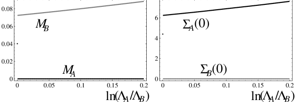
Figure 3: The left hand side is the estimated gauge boson masses and the right hand side is the mass functions $\Sigma_{A}(0)$ and $\Sigma_{B}(0)$ in the case $N_{A}=N_{B}=3$. The horizontal axes are the relative strength of the couplings $\ln(\Lambda_{A}/\Lambda_{B})$. The black points indicate $M_{A}$, $\Sigma_{A}(0)$ and the gray points indicate $M_{B}$, $\Sigma_{B}(0)$. A simple first order phase transition occurs at $\ln(\Lambda_{A}/\Lambda_{B})=0$.

We use a unit scale setting $\Lambda_{B}=1$ and fix the value of $N_{B}$ as $N_{B}=3$ below. We observe three vacua at the point $\Lambda_{A}=\Lambda_{B}$. It is seen, however, that the symmetric vacuum ($\Sigma_{A}=\Sigma_{B}$) is unstable against the perturbation of the couplings. If the symmetric vacuum was one of the stable points of the system, we would have a plateau extending from the point $\Lambda_{A}=\Lambda_{B}$ to $\ln(\Lambda_{A}/\Lambda_{B})>0$ in Fig. 3. We conclude that the symmetric vacuum is an artifact generated by our procedure and is not true vacuum. Then, the correct solution shows a simple first order phase transition at $\ln(\Lambda_{A}/\Lambda_{B})=0$. Here, we notice that both the $SU(N_{A})_{A}$ and $SU(N_{B})_{B}$ broken vacua are stable against any values of $\ln(\Lambda_{A}/\Lambda_{B})$. We recognize this fact by the explicit forms of the coupled Schwinger-Dyson equations (in Eqs. (3.17)). For example, if we use asymmetric initial functions ($\Sigma_{A}(x)\neq 0$ and $\Sigma_{B}(x)\equiv 0$), we will always find the $SU(N_{B})_{B}$ broken vacuum having no dependence of the values of the couplings.

As a result, we have the following phase. In the range $-\infty<\ln(\Lambda_{A}/\Lambda_{B})\leq 0$, the $SU(N_{A})_{A}$ symmetry is broken with the gauge boson mass $M_{A}=f_{B}(0,M_{A})$ and the symmetry $SU(N_{B})_{B}$ is completely manifest. The values of the masses drastically change around the point $\ln(\Lambda_{A}/\Lambda_{B})=0$. In the range $0\leq\ln(\Lambda_{A}/\Lambda_{B})<\infty$, $SU(N_{A})_{A}$ is completely manifest and $SU(N_{B})_{B}$ is broken with $M_{B}=f_{A}(0,M_{B})$. This result shows that the most attractive channel (MAC) hypothesis works completely. The broken $SU(N_{B})_{B}$ gauge interaction can form $SU(N_{A})_{A}$ singlet four-Fermi interaction by introducing $SU(N_{A})_{A}$ singlet fermions. (Notice that $\psi_{R}$ and $\xi_{L}$ cannot form such a four-Fermi interaction.)

In conclusion, we obtain a theory in which $SU(N_{A})_{A}$ Yang-Mills and $SU(N_{B})_{B}$ four-Fermi interactions appear in the low energy region by tuning the couplings such that $\ln(\Lambda_{A}/\Lambda_{B})>0$. There is no fine-tuning. In certain appropriate regions the four-Fermi interaction is in the strong coupling phase necessary for a dynamical symmetry breaking to take place. We will study this in section 5.

Next, let us take different gauge groups; i.e, $N_{A}\neq N_{B}$. We fix the $SU(N_{B})_{B}$ gauge group by setting $N_{B}=3$. We change the value of $N_{A}$ as $N_{A}=5,8,9,10,12$. As for the $N_{A}=5,8$ cases we have first order phase transitions. The phase transition points move to the region $\ln(\Lambda_{A}/\Lambda_{B})>0$ as in Figs. 4 and 5.

However, for the $N_{A}=9$ case we have a second order phase transition as in Fig. 6 at $\ln(\Lambda_{A}/\Lambda_{B})\cong 0.1515$. There are two phase transitions at $\ln(\Lambda_{A}/\Lambda_{B})\cong 0.1515$ and $0.152$, and the latter one seems to be of first order. Second order phase transitions occur clearly in the $N_{A}=10,12$ cases as in Figs. 7 and 8. These models provide asymptotically free gauge theories with additional strong coupling four-Fermi interaction around a second order phase transition point. This is studied in Ref. [12].

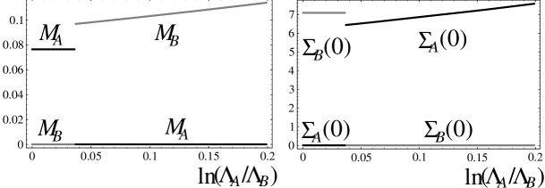
Figure 4: The phase diagram in the case $N_{A}=5$, $N_{B}=3$. A first order phase transition occurs at $\ln(\Lambda_{A}/\Lambda_{B})=0.0355$.

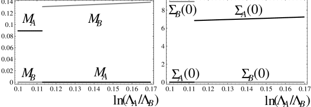
Figure 5: The phase diagram in the case $N_{A}=8$, $N_{B}=3$. A first order phase transition occurs at $\ln(\Lambda_{A}/\Lambda_{B})=0.111$.

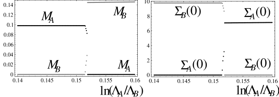
Figure 6: The phase diagram in the case $N_{A}=9$, $N_{B}=3$. Phase transitions occur around $\ln(\Lambda_{A}/\Lambda_{B})=0.151\sim 0.152$. The former one is of second order and the latter one seems to be of first order.

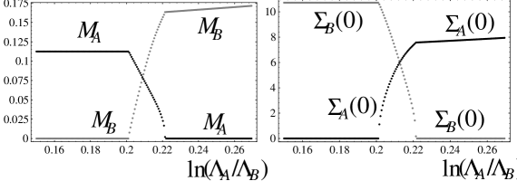
Figure 7: The phase diagram in the case $N_{A}=10$, $N_{B}=3$. Second order phase transitions occur at $\ln(\Lambda_{A}/\Lambda_{B})=0.201,0.222$.

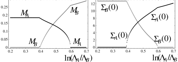
Figure 8: The phase diagram in the case $N_{A}=12$, $N_{B}=3$. Second order phase transitions occur at $\ln(\Lambda_{A}/\Lambda_{B})=0.387,0.597$.

Here we note a fact. If we use a initial condition such that $\Sigma_{A}(x)\equiv 0$ and $\Sigma_{B}(x)\neq 0$, we always have a vacuum where the $SU(N_{A})_{A}$ symmetry is broken and the $SU(N_{B})_{B}$ symmetry is manifest. Similar argument holds for the initial condition such that $\Sigma_{A}(x)\equiv 0$ and $\Sigma_{B}(x)\neq 0$. Namely, we can always have two different solutions specified by $\Sigma_{A}(x)\equiv 0$ and $\Sigma_{B}(x)\equiv 0$, depending on the initial functional forms of the mass function in solving the coupled Schwinger-Dyson equations. This property gives hysteresis curves in phase diagrams if we use particular forms for the initial mass functions.

3 The Coupled Schwinger-Dyson Equations

In this section, we derive the coupled Schwinger-Dyson equations used in the above analysis. Before proceeding, we explain the basic ingredients in the Schwinger-Dyson equations here. The coupled Schwinger-Dyson equations with two massive gauge bosons are specified by the eight parameters in the improved ladder approximation: gauge boson masses $M_{A}$ and $M_{B}$, Yang-Mills interaction scales $\Lambda=\Lambda_{A},\Lambda_{B}$ of the running couplings, one-loop $\beta$ functions $\mu dg/d\mu=\beta(g)=-\beta_{0}g^{3}$ for $g=g_{A},g_{B}$, and the second Casimir invariants $C_{2}(F)$ of the fermion fundamental representations $F=\underline{N}_{A},\underline{N}_{B}$. Here, we are using the Yang-Mills interaction scale for specifying the coupling strengths. When we solve the coupled Schwinger-Dyson equations, one dimensionful parameter out of $M_{A}$, $M_{B}$, $\Lambda_{A}$ and $\Lambda_{B}$ is irrelevant. We regard $\Lambda_{B}$ as a unit scale during the calculation by rescaling all dimensionful parameters in terms of $\Lambda_{B}$. In the present system the coefficient of the $\beta$ function and the second Casimir invariant have different values in the two Schwinger-Dyson equations. Namely, $\beta_{A0}=(11N_{A}-2N_{B})/(3\cdot 16\pi^{2})$, $\beta_{B0}=(11N_{B}-2N_{A})/(3\cdot 16\pi^{2})$ and $T^{a}_{X}T^{a}_{X}=C_{2}(\underline{N}_{X})=(N_{X}^{2}-1)/(2N_{X})$ for $X=A,B$.

Now, let us write down the coupled Schwinger-Dyson equations. The fermion propagator is defined by

$$S_{F}=\left(\begin{array}[]{ccc}\langle\psi_{R}\overline{\psi}_{R}\rangle&\langle\psi_{R}\overline{\xi}_{L}\rangle&\langle\psi_{R}\overline{\eta}_{L}\rangle\\ \langle\xi_{L}\overline{\psi}_{R}\rangle&\langle\xi_{L}\overline{\xi}_{L}\rangle&\langle\xi_{L}\overline{\eta}_{L}\rangle\\ \langle\eta_{L}\overline{\psi}_{R}\rangle&\langle\eta_{L}\overline{\xi}_{L}\rangle&\langle\eta_{L}\overline{\eta}_{L}\rangle\end{array}\right)~{}.$$ (3.6)

We note that the free fermion propagator is given by

$$S_{F0}(p)=\frac{i}{\alpha^{\mu}p_{\mu}}~{},$$ (3.7)

where we define generalized $\sigma$ matrices as

$$\alpha^{\mu}=\left(\begin{array}[]{ccc}\overline{\sigma}^{\mu}&0&0\\ 0&\sigma^{\mu}&0\\ 0&0&\sigma^{\mu}\end{array}\right)~{},~{}~{}\overline{\alpha}^{\mu}=\left(\begin{array}[]{ccc}\sigma^{\mu}&0&0\\ 0&\overline{\sigma}^{\mu}&0\\ 0&0&\overline{\sigma}^{\mu}\end{array}\right)~{},$$ (3.8)

with

$$\overline{\sigma}^{\mu}=\sigma_{\mu}=\left(\left(\begin{array}[]{cc}1&0\\ 0&1\end{array}\right),\left(\begin{array}[]{cc}0&1\\ 1&0\end{array}\right),\left(\begin{array}[]{cc}0&-i\\ i&0\end{array}\right),\left(\begin{array}[]{cc}1&0\\ 0&-1\end{array}\right)\right)~{}.$$ (3.9)

Then, the Schwinger-Dyson equation is given by

$$iS_{F0}^{-1}(p)-iS_{F}(p)^{-1} = \int\frac{d^{4}k}{(2\pi)^{4}i}\,g_{A}^{2}(-p^{2}\!-\!k^{2})\,\alpha^{\mu}T^{a}_{A}\,iS_{F}(k)\,\alpha^{\nu}T^{a}_{A}\,K_{\mu\nu}(p-k;M_{A})$$

$$+ \int\frac{d^{4}k}{(2\pi)^{4}i}\,g_{B}^{2}(-p^{2}\!-\!k^{2})\,\alpha^{\mu}T^{a}_{B}\,iS_{F}(k)\,\alpha^{\nu}T^{a}_{B}\,K_{\mu\nu}(p-k;M_{B})~{}.$$

The generators $T^{a}_{A}$ and $T^{a}_{B}$ eliminate $SU(N_{A})_{A}$ and $SU(N_{B})_{B}$ singlet states, respectively. The propagator $K_{\mu\nu}(l;M)$ of a massive gauge boson in a Landau-like gauge[18] is given by

$$K_{\mu\nu}(l;M)=\frac{1}{M^{2}-l^{2}}\left(g_{\mu\nu}+\frac{l_{\mu}l_{\nu}}{M^{2}-l^{2}}\right)~{}.$$ (3.11)

The quantity $g_{X}^{2}(\mu^{2})$ ($X=A,B$) is the running coupling having a threshold scale at the gauge boson mass $\mu=M_{X}$. There is no need to regularize the running coupling $g_{X}^{2}$ below the scale $\Lambda_{X}$ if $M_{X}>\Lambda_{X}$, since the running of $g_{X}^{2}$ stops below the scale $M_{X}$. Then, $g_{X}^{2}$ takes the form

$$g_{X}^{2}(\mu^{2})=\frac{1}{\beta_{X0}\ln(\max(\mu^{2},M_{X}^{2})/\Lambda_{X}^{2})}~{},$$ (3.12)

when we work in $M_{X}>\Lambda_{X}$. In the cases with a massless gauge boson the running coupling should be regularized, and various forms[19, 20, 21] may be taken. When we work in $M_{X}\leq\Lambda_{X}$, we adopt the following form[20, 4]

$$g_{X}^{2}(\mu^{2})=\frac{1}{\beta_{X0}}\times\left\{\begin{array}[]{ll}\displaystyle\frac{1}{t}&\mbox{ if $t_{F}<t$ }\vskip 3.0pt plus 1.0pt minus 1.0pt\\ \displaystyle\frac{1}{t_{F}}+\frac{(t_{F}-t_{C})^{2}-(t-t_{C})^{2}}{2t_{F}^{2}(t_{F}-t_{C})}&\vskip 3.0pt plus 1.0pt minus 1.0pt\mbox{ if $t_{C}<t<t_{F}$ }\\ \displaystyle\frac{1}{t_{F}}+\frac{(t_{F}-t_{C})}{2t_{F}^{2}}&\mbox{ if $t<t_{C}$ }\vskip 3.0pt plus 1.0pt minus 1.0pt\end{array}\right.~{},$$ (3.13)

where $X=A,B$, $t=\ln(\max(\mu^{2},M_{X}^{2})/\Lambda_{X}^{2})$ and we fix $t_{F}=0.15$ and $t_{C}=-2.0$.

Next, let us transform the SD equation in a component form. We have vanishing condensates between the Weyl fermions with the same chiralities:

$$\langle\overline{\psi}_{R}\psi_{R}\rangle=\langle\overline{\xi}_{L}\xi_{L}\rangle=\langle\overline{\eta}_{L}\eta_{L}\rangle=\langle\overline{\xi}_{L}\eta_{L}\rangle=\langle\overline{\eta}_{L}\xi_{L}\rangle\equiv 0~{}.$$ (3.14)

Then, the non-trivial condensates are $\langle\overline{\psi}_{R}\xi_{L}\rangle=\langle\overline{\xi}_{L}\psi_{R}\rangle$ and $\langle\overline{\psi}_{R}\eta_{L}\rangle=\langle\overline{\eta}_{L}\psi_{R}\rangle$, where the condensates are taken as real numbers by using phase transformations of the fermion fields. Then, the mass function takes the form

$$\Sigma=\left(\begin{array}[]{ccc}0&1_{B+\xi}\Sigma_{A}&1_{A+\eta}\Sigma_{B}\\ 1_{B+\xi}\Sigma_{A}&0&0\\ 1_{A+\eta}\Sigma_{B}&0&0\end{array}\right)~{},$$ (3.15)

where $1_{B+\xi}$ and $1_{A+\eta}$ are $N_{B}\times N_{B}$ and $N_{A}\times N_{A}$ unit matrices, respectively. In the Landau-like gauge the wave function renromalizations are expected to be small, then the fermion propagator is given by

$$S_{F}(p)=\frac{i}{\alpha^{\mu}p_{\mu}-\Sigma(-p^{2})}=(\overline{\alpha}^{\mu}p_{\mu}+\Sigma(-p^{2}))\frac{-i}{\Sigma(-p^{2})-p^{2}}{}~{}.$$ (3.16)

Substituting Eq. (3.16) into Eq. (LABEL:eq:coupledSD) and carrying out the four-dimensional angle integrations, we find the coupled Schwinger-Dyson equations in component form

$$\Sigma_{A}(x) = \int_{0}^{\infty}\!ydyK_{A}(x,y)\frac{\Sigma_{A}(y)}{y+\Sigma_{A}(y)^{2}+\Sigma_{B}(y)^{2}}{}~{},$$

$$\Sigma_{B}(x) = \int_{0}^{\infty}\!ydyK_{B}(x,y)\frac{\Sigma_{B}(y)}{y+\Sigma_{A}(y)^{2}+\Sigma_{B}(y)^{2}}~{},$$ (3.17)

where the kernel $K_{X}$ ($X=A,B$) is given by

$$K_{X}(x,y)=\frac{\lambda_{X}(x+y)}{x+y+M_{X}^{2}+\sqrt{(x+y+M_{X}^{2})^{2}-4xy}}\left(3+\frac{M_{X}^{2}}{\sqrt{(x+y+M_{X}^{2})^{2}-4xy}}\right){}~{},$$ (3.18)

with

$$\lambda_{X}(x)\equiv\frac{C_{2}(\underline{N}_{X})g_{X}^{2}(x)}{8\pi^{2}}~{}.$$ (3.19)

4 Nambu-Goldstone Boson and its Decay Constant

In this section we briefly show how the NG boson couples to the gauge current with the decay constant and we derive a generalized Pagels-Stokar formula in the present system. In this paper instead of solving the BS equation for the NG boson $\pi_{A}$ we use a convenient approximation by Pagels and Stokar[22], in which the BS amplitude is entirely given by the mass function. If we omit the interference effect of the other mass function, our formula reduces to the usual Pagels-Stokar formula[22] up to an overall factor.

In order for the argument to be transparent we concentrate on the dynamical symmetry breaking of the gauge group $SU(N_{B})_{B}$. The Noether current of $SU(N_{B})_{B}$ is given by

$$J_{B}^{b\mu}=\overline{\psi}_{R}\overline{\sigma}^{\mu}T_{B}^{b}\psi_{R}+\overline{\eta}_{L}\sigma^{\mu}T_{B}^{b}\eta_{L}~{},$$ (4.20)

where $T_{B}^{b}$ is the generator of $SU(N_{B})_{B}$. The NG boson $\pi_{A}$ couples to the first part of this current (4.20), and also couples to the left Weyl spinor current, as

$$\langle 0|\overline{\psi}_{R}\overline{\sigma}^{\mu}T_{B}^{b}\psi_{R}|\pi_{A}^{a}(q)\rangle = i\delta^{ab}q^{\mu}~{}f_{A}$$

$$\langle 0|\overline{\xi}_{L}\sigma^{\mu}T_{\xi}^{b}\xi_{L}|\pi_{A}^{a}(q)\rangle = -i\delta^{ab}q^{\mu}~{}f_{A}~{}.$$ (4.21)

where $f_{A}$ is its decay constant.

The BS amplitude of the NG boson $\pi_{A}$ is defined by

$$\langle 0|T\Psi_{i}(x/2)\overline{\Psi}_{j}(-x/2)|\pi_{A}^{a}(q)\rangle\equiv 1_{A}\;T_{B+\xi}^{a}\;\int\!dxe^{-ipx}\chi_{Aij}(p;q){}~{},$$ (4.22)

where $\Psi=(\psi_{R},\xi_{L},\eta_{L})$ and $1_{A}$ is the $N_{A}\times N_{A}$ unit matrix and denotes $SU(N_{A})_{A}$ gauge singlet. The truncated BS amplitude $\widehat{\chi}_{A}^{a}(p;q)$ is defined by

$$\widehat{\chi}_{A}^{a}(p;q)=S_{F}^{-1}(p+q/2)\,\chi_{A}^{a}(p;q)\,S_{F}^{-1}(p-q/2)~{}.$$ (4.23)

Then, from Eqs. (4.21) and (4.22) the decay constant $f_{A}$ is expressed in terms of the truncated BS amplitude $\widehat{\chi}_{A}$ as

$$q^{\mu}~{}f_{A}=\frac{N}{2}\int\!\frac{d^{4}p}{(2\pi)^{4}i}~{}{\rm tr}\;\overline{\sigma}^{\mu}\Big{[}iS_{F}(p+q/2)\;\widehat{\chi}_{A}(p;q)\;iS_{F}(p-q/2)\Big{]}_{11}~{}.$$ (4.24)

The chiral Ward-Takahashi identity for the “external” symmetry $SU(N_{B})_{B}\times SU(N_{B})_{\xi}$ is given by

$$-iq^{\mu}\Gamma_{A\mu}^{a}(p;q)=T_{B+\xi}^{a}\left(S_{F}^{-1}(p+q/2)\gamma_{5}^{\prime}-\gamma_{5}^{\prime}S_{F}^{-1}(p-q/2)\right){}~{},$$ (4.25)

where $\gamma_{5}^{\prime}=\mbox{diag.}(1,-1,0)$. The NG boson $\pi_{A}^{a}$ couples to this vertex function as

$$\Gamma_{A\mu}^{a}(p;q)\sim-2f_{A}\,T_{B+\xi}^{a}\;\widehat{\chi}(p;q)\;\frac{q_{\mu}}{q^{2}}+\cdots~{}.$$ (4.26)

Using Eqs. (4.25) and (4.26), the truncated BS amplitude is given in terms of the mass function in the soft momentum limit $q_{\mu}\rightarrow 0$:

$$T_{B+\xi}^{a}\widehat{\chi}_{A}^{a}(p;0)=\frac{T_{B+\xi}^{a}}{f_{A}}\left(\begin{array}[]{ccc}0&-\Sigma_{A}(-p^{2})&0\\ \Sigma_{A}(-p^{2})&0&0\\ 0&0&0\end{array}\right)~{}.$$ (4.27)

In the Pagels-Stokar approximation we use the amputated BS amplitude in the soft momentum limit instead of the full one. Substituting Eq. (4.27) into Eq. (4.24) and expanding the propagators in terms of $q_{\mu}$, we finally find

$$f_{A}^{2}=\frac{N_{A}}{16\pi^{2}}\int_{0}^{\infty}\!xdx\;\Sigma_{A}(x)$$ (4.28)

$$\times \frac{\Sigma_{A}(x)\left(1+\frac{\displaystyle 4x\Sigma_{B}^{\prime}(x)\Sigma_{B}(x)-\Sigma_{B}(x)^{2}}{\displaystyle 8x}\right)-\frac{\displaystyle x}{\displaystyle 2}\Sigma^{\prime}_{A}(x)\left(1+\frac{\displaystyle\Sigma_{B}(x)^{2}}{\displaystyle 2x}\right)}{x+\Sigma_{A}(x)^{2}+\Sigma_{B}(x)^{2}}~{}.$$

The above arguments similarly hold for the dynamical breaking of the gauge symmetry $SU(N_{A})_{A}$, and we obtain a similar formula for $f_{B}$.

5 Broken Dynamics in the Strong Coupling Phase and the large anomalous dimension $\gamma_{m}$

In section 2 we find phase diagrams ($N_{A}\leq 9$) in which a broken dynamics cannot break the other gauge symmetry. In this section we study whether the broken dynamics is in a strong coupling phase enough to break the $SU(2)_{L}$ symmetry. For definiteness we consider the case where the symmetry $SU(N_{A})_{A}$ is manifest and the symmetry $SU(N_{B})_{B}$ is broken dynamically, and we put $N_{B}=3$. The topcolor gauge symmetry may be this $SU(3)_{B}$. We consider the case when the $SU(2)_{L}$ gauge interaction is relatively weak enough for us to regard it as a global symmetry.

Let us consider three Weyl fermions which are $SU(N_{A})_{A}$ singlet. The fermions have the following charge:

$$\begin{array}[]{c|cc}&SU(3)_{B}&SU(2)_{L}\\ \hline\cr q_{L}&3&2\\ t_{R}&3&1\\ b_{R}&3&1\end{array}$$ (5.29)

The following analysis is devoted to make clear whether the condensates $\langle\overline{t}_{R}q_{L}\rangle=\langle\overline{b}_{R}q_{L}\rangle$ form and break the $SU(2)_{L}$ symmetry.

The Schwinger-Dyson equation is simple and determines the propagator of the fermions $q_{L}$ and $q_{R}$. We use the notations $q_{L}^{i}\equiv(t_{L},b_{L})^{T}$ and $q_{R}^{i}\equiv(t_{R},b_{R})^{T}$. We use the improved ladder approximation and the Landau-like gauge[18]. The Dirac fermion $q$ respects the $SU(2)_{L+R}$ custodial symmetry, and the propagator takes the form

$$\langle q^{i}(x)\overline{q}_{j}(0)\rangle\equiv\delta^{i}_{j}S_{F}(x)~{}.$$ (5.30)

The Dirac fermion propagator is expanded into two invariant amplitudes as

$$iS_{F}^{-1}(p)=A(-p^{2}){p}\kern-6.0pt\mbox{\it/}-B(-p^{2})~{}.$$ (5.31)

The Schwinger-Dyson equation determines the invariant amplitudes $A(x)$ and $B(x)$, where $x\equiv-p^{2}$.

If we work with the massless gauge boson $M_{B}=0$, the amplitudes $A(x)$ is identical to unity, which is shown after the four dimensional angle integration. Even when we work with $M_{B}\neq 0$, it is verified in Ref. [23] that $A(x)\simeq 1$ by an explicit numerical calculation in the fixed coupling case. In the high energy region $A(x)$ must converge to unity quickly enough, otherwise the resultant Dirac fermion propagator will be inconsistent with the result by the operator product expansion and the renormalization group analysis. It means an explicit breaking of the chiral gauge symmetries in the present system.[19, 24] In this paper, we put $A(x)=1$ for simplicity although the coupling is running. It should not modify the physical consequences of this paper.

Then, the Schwinger-Dyson equation takes the form

$$\Sigma(x)=\int_{0}^{\infty}\!xdx\;K_{B}(x,y)\frac{\Sigma(y)}{y+\Sigma(y)^{2}}~{}.$$ (5.32)

After obtaining the fermion propagator $S_{F}(p)$, we estimate the decay constant $f_{t}$ of the NG boson $\pi_{t}^{a}$ by using the Pagels-Stokar formula[22] which is given by

$$f_{t}^{2}=\frac{3}{16\pi^{2}}\int_{0}^{\infty}\!xdx\;\Sigma(x)\frac{\Sigma(x)-x\Sigma^{\prime}(x)/2}{x+\Sigma(x)^{2}}~{}.$$ (5.33)

We regard the decay constant as a function of $M_{B}$; i.e., $f_{t}=f_{t}(M_{B})$. We show the decay constant $f_{t}(M_{B})$ in Fig. 9.

Figure 9: The decay constant $f_{t}$ as a function of the gauge boson mass $M_{B}$. Unit is $\Lambda_{B}$. In the case $M_{B}>\Lambda_{B}$, the decay constant can be calculated without regularizing the infrared form of the running coupling. The phase transition occurs at $M_{B}=1.16\Lambda_{B}$ with second order.

The decay constant is evaluated with $M_{B}>\Lambda_{B}$, where we put $\Lambda_{B}=1$. This result has no ambiguity stemming from any regularized form of the running coupling in the infrared region lower than the interaction scale $\Lambda_{B}$. This is in contrast with the result in Ref. [20]. Above the critical mass $M_{B}>f_{t}^{-1}(0)=1.16\Lambda_{B}$ the chiral symmetry is restored. Near the phase transition point ($M<f_{t}^{-1}(0)$) with a small dynamical mass of the Dirac fermion, the anomalous dimension $\gamma_{m}$ approaches that of the Nambu-Jona-Lasinio model:

$$\gamma_{m}\equiv-\frac{d}{d\ln\mu}\ln|\langle\overline{q}q\rangle|\cong\frac{d}{d\ln M_{B}}\ln|\langle\overline{q}q\rangle|=2~{},$$ (5.34)

in the low energy region $\mu<\!<M_{B}$. Here the gauge boson mass $M_{B}$ plays the role of the cutoff. We conclude that the renormalizable theory, considered here, provides the large anomalous dimension $\gamma_{m}\cong 2$ just below the critical point $M_{B}\cong f_{t}^{-1}(0)$ in the low energy region.

Next, let us proceed to the lower region $M_{B}<\Lambda_{B}$. We can guess that $f_{t}(M_{B})$ will be a constant in $M_{B}<\Lambda_{B}$, since such a mass $M_{B}$ smaller than $\Lambda_{B}$ should be negligible in the gauge interaction dynamics. This is also confirmed empirically. If we convert the value $f_{t}(\Lambda_{B})/\Lambda_{B}$ to the ordinary QCD case by multiplying by a necessary factor, it already saturates the experimental value $93~{}[\mbox{MeV}]/\Lambda_{QCD}$ of the actual pion. Therefore, we should keep the property $f_{t}(M_{B})\sim\mbox{const.}$ ($M_{B}<\Lambda_{B}$) when we regularize the running coupling in the infrared region.

Figure 10: The decay constant $f_{t}$ is plotted as a function of the gauge boson mass $M_{B}$ in Fig. (a). The mass function of the top quark is plotted in Fig. (b). The unit is in $\Lambda_{B}$. As mentioned in Fig. 9 the phase transition occurs at $M_{B}=1.16\Lambda_{B}$.

We adopt the form (3.13). Of course we should use the same coupling as that used in Eq. (LABEL:eq:coupledSD). Above the scale $\mu^{2}=\exp t_{F}$ the functional form is exactly the same as that of the one-loop running coupling, below the scale $\mu^{2}=\exp t_{F}$ the running coupling is regularized by using the second order polynomial in $t=\ln\mu^{2}$ and in the low energy region $t\leq t_{C}$ the coupling becomes a constant. The running coupling with $t_{F}=0.15$ agrees with the one-loop running coupling form over almost of the range of $t$ greater than the interaction scale $\Lambda_{B}$. The smaller value of $t_{F}$ would be good but increases the error in numerical calculations. The result of $f_{t}(M_{B})$ is shown in Fig. 10. We should notice that the functional form above $M_{B}^{2}\geq\exp t_{F}\simeq 1.16$ in Fig. 10 is exactly the same as that in Fig. 9, and is perfectly independent on the infrared regularization of the running coupling, since the running of the coupling stops below the threshold $M_{B}^{2}$ which is just above the regularized scale $\exp t_{F}$. We observe that $f_{t}(0)=0.0722$ and $f_{t}(\Lambda_{B})=0.0675$. So, the decay constant squared $f_{t}$ does not change by more than 7% in the range $0<M_{B}<\Lambda_{B}$.

Acknowledgements

We would like to thank T. Kugo for enlightening suggestion, discussions and comments. We are grateful to M.E. Peskin for discussions and suggestions. We are also grateful to K. Higashijima and T. Maskawa for comments. We would like to thank A. Bordner for correcting English. We also thank Y. Kikukawa, N. Maekawa and K. Nakanishi for discussions.

References

[1]
S. Weinberg,
Phys. Rev.D13 (1976) 974;
D19 (1979) 1277.
L. Susskind,
Phys. Pev.D20 (1979) 2619.
and for a review see
E. Farhi and L. Susskind,
Phys. Rep.74 (1981) 227.
[2]
Y. Nambu,
in New Trends in Strong Coupling Gauge Theories, 1988
International Workshop, Nagoya, Japan, ed. by M.Bando, T.Muta
and K.Yamawaki (World Scientific, Singapore, 1989);
EFI Peport No. 89-08, 1989 (unpublished);
V.A. Miransky, M. Tanabashi and K. Yamawaki,
Phys. Lett.B221 (1989) 177;
Mod. Phys. Lett.62 (1989) 2793;
W. Marciano,
Phys. Rev. Lett.62 (1989) 2793;
W.A. Bardeen, C.T. Hill and M. Lindner,
Phys. Rev.D41 (1990) 1647.
[3]
M.E. Peskin and T. Takeuchi,
Phys. Rev. Lett.65 (1990) 964;
Phys. Rev.D46 (1992) 381;
G. Altarelli and R. Barbieri,
Phys. Lett.B253 (1991) 161.
[4]
M. Harada and Y. Yoshida,
Phys. Rev.D50 (1994) 6902.
[5]
R. Barbieri, M. Frigeni, F. Giuliani and H.E. Haber,
Nucl. Phys.B341 (1990) 309.
[6]
N. Maekawa,
preprint TU-460, Jun 1994, hep-ph/9406375.
[7]
S. Dimopoulos, S. Raby and P. Sikivie,
Nucl. Phys.B176 (1980) 449;
S. Dimopoulos and J. Ellis,
Nucl. Phys.B182 (1981) 505.
[8]
S. Dimopoulos and L. Susskind,
Nucl. Phys.B155 (1979) 237;
E. Eichten and K.D. Lane,
Phys. Lett.90B (1980) 125.
[9]
V.A. Miransky, M. Tanabashi and K. Yamawaki,
in Ref. [2]
[10]
R.R. Mendel and V.A. Miransky,
Phys. Lett.B268 (1991) 384;
C.T. Hill,
Phys. Lett.B345 (1995) 483, hep-ph/9411426.
[11]
C.T. Hill, in Ref. [10];
R.S. Chivukula, B.A. Dobrescu and J. Terning,
preprint BUHEP-95-08, Mar 1995, hep-ph/9503203.
[12]
V.A. Miransky and K. Yamawaki,
Mod. Phys. Lett.A4 (1989) 129;
V.A. Miransky, T. Nonoyama and K. Yamawaki,
Mod. Phys. Lett.A4 (1989) 1409.
[13]
M.A. Luty,
Phys. Rev.D48 (1993) 1295.
[14]
H. Georgi,
Nucl. Phys.B156 (1979) 126.
[15]
S. Raby, S. Dimopoulos and L. Susskind,
Nucl. Phys.B169 (1980) 373.
[16]
C. Vafa and E. Witten,
Nucl. Phys.B234 (1984) 173.
[17]
R. Jackiw and K. Johnson,
Phys. Rev.D8 (1973) 2386.
[18]
T. Maskawa and H. Nakajima,
Prog. Theor. Phys.52 (1974) 1326;
Prog. Theor. Phys.54 (1975) 860.
[19]
K. Higashijima,
Phys. Rev.D29 (1984) 1228.
[20]
K. Aoki, M. Bando, T. Kugo, M.G. Mitchard and H. Nakatani,
Prog. Theor. Phys.84 (1990) 683.
[21]
T. Kugo, M.G. Mitchard and Y. Yoshida,
Prog. Theor. Phys.91 (1994) 521.
[22]
H. Pagels and S. Stokar, Phys. Rev.D20 (1979) 2947.
[23]
K.-I. Kondo,
Phys. Lett.B226 (1989) 329.
[24]
A. Cohen and H. Georgi,
Nucl. Phys.B314 (1989) 7.