Double Pomeron Jet Cross Sections

Abstract

We treat hadron-hadron collisions where the final state is kinematically of the kind associated with double-pomeron-exchange (DPE) and has large transverse momentum jets. We show that in addition to the conventional factorized (FDPE) contribution, there is a non-factorized (NDPE) contribution which has no pomeron beam jet. Within a simple model we compute DPE-two-jet total and differential cross sections at Tevatron energy scales, and show that the NDPE contribution is dominant.

When two hadrons collide at high energy, there is about a 10% chance that one of the incoming hadrons will survive into the final state, while losing only a small fraction of its energy. Such events are called diffractive. The object that is exchanged in diffractive processes is called the “pomeron”. A primary characteristic is that cross sections with pomeron exchange are approximately independent of energy at high energy; the pomeron has spin close to unity [1]. Moreover, there has been growing experimental evidence that within diffractive events, hard QCD processes can also occur, i.e., processes with a large momentum transfer. Such “diffractive hard scattering” has been been seen not only in hadron-hadron scattering by the UA1 and UA8 experiments [2, 3], but also in electron-proton scattering at the H1[4] and ZEUS[5] experiments, both in the deep-inelastic regime and in photoproduction.

An interesting class of diffractive hadron-hadron collisions, is where both hadrons survive unscathed, but leave a remnant system in the central region of final-state rapidity. Such events are called double-pomeron exchange (DPE) events [6, 7]. In effect, one can try to consider such processes as pomeron-pomeron collisions. Our purpose in this paper is to explore the properties of jet production in DPE events, and in particular the breakdown of hard-scattering factorization. Jet production by DPE has been reported [8] in the UA1 detector.

The simplest model for diffractive hard scattering is due to Ingelman and Schlein [9]. They treat each exchanged pomeron as a particle, in the same manner as one obtains photoproduction cross sections from electron-hadron scattering at small momentum transfer. Diffractive hard scattering is then obtained by the use of parton densities in the pomeron. The model is used in much phenomenology [4, 5], and has been applied to DPE[10]. Interestingly, as Collins, Frankfurt and Strikman (CFS) [11, 12] explained, the Ingelman-Schlein model is not valid in QCD, even though the model forms a useful phenomenological benchmark [13]. CFS also predict a specific signature of the breakdown of factorization, that at the leading twist level all the momentum of the pomeron can go into the hard scattering—the process is “super-hard” or “lossless”. UA8 [3] data gives experimental support to this result.

Our present paper shows how the mechanism of Collins, Frankfurt and Strikman applied to DPE at the level of lowest-order Feynman graphs provides a striking mechanism for the breakdown of factorization, and we turn it into a quantitative, if crude, model The model is in effect a version of the Low-Nussinov-Gunion-Soper model [15], and the same model was used by Berera and Soper [16] to understand properties of the pomeron’s structure function. We will calculate the cross section for jet production in DPE. The important free parameter in our model is an overall normalization which can be determined from elastic scattering. Pumplin [17] has done some calculations in the same model, but without the strongly dominant gluon-gluon subprocess. We call the model non-factorizing double-pomeron-exchange (NDPE), to contrast it with the Ingelman-Schlein model applied to DPE, which we call factorized double-pomeron-exchange (FDPE).

The dramatic feature of our model is that the pomerons have no beam jets; the final state is then exceptionally clean, because it consists of the two isolated, diffracted hadrons, the high transverse-momentum jets, and nothing else. Not only are such processes theoretically interesting in their own right, but they have advantages for certain kinds of new particle searches, provided the cross section is high enough, because a lot of the background event is no longer present. Production processes of heavy flavors and Higgs are two such examples. But studies of hard scattering in DPE should surely start with the simplest processes, jet production.

Schäfer, Nachtmann and Schöpf [18] have characterized the final states we calculate as “exclusive” production , with the Ingelman-Schlein process being a corresponding “inclusive” process.

Although there has been a significant amount of work on hard processes with DPE, almost all of it has concerned production of heavy quarks and Higgs bosons — see, for example, Refs. [10, 18, 19]. Moreover, much of it has used the Ingelman-Schlein method, the FDPE process, which, as we will see, is much smaller than the NDPE process. The only work on the DPE-to-jets process that we know of is by Pumplin [17]. He used the same model as we did, but restricted his attention to the production of quark jets. As we will show in Sect. VI A, production of quark jets is very much smaller than the production of gluon jets, because it has a zero at zero momentum transfer. On the other hand, Pumplin paid more attention to good modeling of the proton’s elastic form factor.

Donnachie and Landshoff [20] have developed an extensive phenomenology of a two-gluon model for the pomeron. Bialas and Landshoff [19] used this model to calculate Higgs production by DPE. This model has many similarities to ours, and it includes better modeling of the non-perturbative part of the process. In particular, it has a more precise treatment of the pomeron-proton vertex and of the pomeron trajectory.

However, there is one important principle that our model establishes. This is that the exclusive processes of DPE to jets is leading twist. This is quite non-trivial, since in proving factorization, there are some very non-trivial cancellations [21]. Indeed some of our graphs are a power law larger than the final answer. The proof of the necessary cancellation relies on Ward identities applied to the hard part, as we demonstrate around Eq. (23) below. To show that general principles do not imply some other cancellation, it is important to have a complete, consistent and gauge-invariant model. This is provided by our model, which consists of all the lowest-order Feynman graphs that follow from a certain toy Lagrangian.

Our work also shows that one only has to be concerned about this kind of cancellation in the hard scattering part of the graphs. It also indicates what principles need to be applied in a general process. Without taking the cancellations into account, the calculation of the Feynman graphs is much less efficient than it need be. Of course, once these results have been established, one is free to do more precise modeling of the bound state.

Lu and Milana [22] have also calculated Higgs production by DPE, but they did not realize that there is a factorization-breaking mechanism. Hence their cross section is too small, by orders of magnitude.

I Kinematics

The process we are interested in is

$$A+B\rightarrow A^{\prime}+B^{\prime}+\mbox{\rm 2 jets}.$$ (1)

The hadrons $A$ and $B$ lose tiny fractions $x_{a}$ and $x_{b}$ of their respective longitudinal momenta, and they acquire transverse momenta ${\bf Q}_{1}$ and ${\bf Q}_{2}$. (This defines a diffractive regime, and in Regge theory would lead to an expectation of the dominance of double pomeron exchange (DPE) — Fig. 1.) The jets carry large momenta of magnitude $E_{T}$ in the plane perpendicular to the collision axis with azimuthal angle $\phi$. (This defines a hard-scattering regime.) The small transfer of longitudinal momentum to the hard process implies large rapidity gaps between the jets and the two outgoing hadrons. In what follows, we will generically denote the hadronic scale by $m$. We are interested in the kinematic region where $m$, ${\bf Q}_{1}$, and ${\bf Q}_{2}$ are of a typical hadronic scale (less than about 1 GeV), while $E_{T}$ is much greater than this scale, but much less than $\sqrt{s}$.

FIG. 1.: Double pomeron exchange (DPE) to two jets.

To understand the asymptotics of Feynman graphs for our process, it is convenient to use light-cone components $(+,-;{\bf\perp})$. The components of momenta of the hadrons in Fig. 1 are

$$P_{A} = \left(\sqrt{\frac{s}{2}},\frac{M^{2}}{\sqrt{2s}};{\bf 0}\right)$$ (2)

$$P_{B} = \left(\frac{M^{2}}{\sqrt{2s}},\sqrt{\frac{s}{2}};{\bf 0}\right)$$ (3)

$$P_{A^{\prime}} = \left((1-x_{a})\sqrt{\frac{s}{2}},\frac{(M^{2}+{\bf Q}_{1}^{2})}{(1-x_{a})\sqrt{2s}},{\bf Q}_{1}\right)$$ (4)

$$P_{B^{\prime}} = \left(\frac{(M^{2}+{\bf Q}_{2}^{2})}{(1-x_{b})\sqrt{2s}},(1-x_{b})\sqrt{\frac{s}{2}};{\bf Q}_{2}\right).$$ (5)

We use bold-face type to indicate two-dimensional transverse vectors. For the jets, we ignore terms of relative order $\ll 1$ to get:

$$p_{1} = \left(ax_{a}\sqrt{\frac{s}{2}},bx_{b}\sqrt{\frac{s}{2}};E_{T}\cos\phi,E_{T}\sin\phi\right)$$ (6)

$$p_{2} = \left(bx_{a}\sqrt{\frac{s}{2}},ax_{b}\sqrt{\frac{s}{2}};-E_{T}\cos\phi,-E_{T}\sin\phi\right),$$ (7)

where it is convenient to define

$$a \equiv \frac{1+\sqrt{1-\kappa}}{2},$$ (8)

$$b \equiv 1-a,$$ (9)

with

$$\kappa\equiv\frac{4E^{2}_{T}}{x_{a}x_{b}s}.$$ (10)

We are interested in the limit where $x_{a},x_{b}\rightarrow 0$, to give a Regge-style limit, and where $E_{T}\to\infty$, to give a hard scattering limit. We hold $\kappa$, ${\bf Q}_{1}$, and ${\bf Q}_{2}$ fixed, to correspond to a fixed angle for the hard scattering and fixed transverse momenta for the outgoing hadrons. In this limit, $s$ necessarily goes to infinity, since it is proportional to $E_{T}^{2}/x_{a}x_{b}$.

II Model

Our method is that of Berera and Soper [16]. We model the process by the lowest order Feynman graphs that are appropriate. The pomerons are replaced by two-gluon exchanges, while instead of true bound states, we model the hadrons by elementary color-singlet scalar particles that we will call “mesons” and that are coupled to scalar quarks by a $\phi^{3}$ coupling.

We normalize the coupling of our mesons so that we reproduce the measured value for cross section for small angle elastic scattering of protons, when we use two-gluon exchange for elastic scattering. This is essentially the Low-Nussinov-Gunion-Soper model [15], but with some simplifications that should not change the relative sizes of the cross sections too much. (We will address the adequacy of our approximations in Sect. VII.)

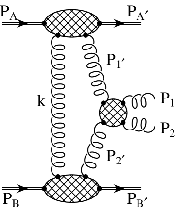
FIG. 2.: Our model of the non-factorizing Double-Pomeron-Exchange (NDPE) amplitude with two gluon jets produced.

Our model for jet production by double pomeron exchange (DPE) is therefore given by Fig. 2. Two gluons couple to each of the diffracted hadrons: this is the minimum number of gluons that can couple to a color-singlet. The top and bottom bubbles imply a sum over all one loop graphs with a quark loop — Fig. 3. One pair of gluons scatters to make the two jets, as in Fig. 4. Note that since the mesons are color-singlet, the jet pair is color singlet and hence Fig. 4 does not include the graph with an $s$-channel gluon. Also in Fig. 3 the graph with a two-gluon two-quark contact interaction is omitted, since, as we will see after Eq. (15), this graph gives a non-leading contribution in the Regge limit. .

For our purposes, the most essential feature of the pomeron is that it gives cross sections that are approximately independent of the center of mass energy $\sqrt{s}$, when $\sqrt{s}$ is made large with all transverse momenta fixed in size. Such behavior is given by exchanges of spin-1 fields — see[1]. Thus, in a perturbative model, the lines coupling bubbles with very different rapidities must all be gluons, exactly as in Fig. 2. Exchange of a quark-antiquark pair instead of a gluon pair would give an amplitude suppressed by a power of $s$. Moreover, for the same reason, the two-gluon form factors in Fig. 2 must be between the meson pairs $(A,A^{\prime})$ and $(B,B^{\prime})$, rather than between the pairs $(A,B^{\prime})$ and $(B,A^{\prime})$.

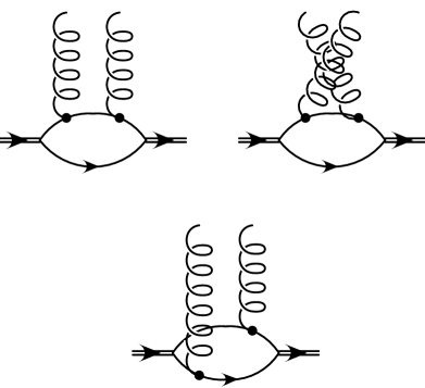
FIG. 3.: Model for two-gluon form factor of meson. There are three other graphs identical to the above, except with the arrows on the quark lines reversed.

FIG. 4.: Graphs for $g+g\to\mbox{\rm jet}+\mbox{\rm jet}$, when the jets are gluon jets, given that the jet pair is color-singlet. Similar graphs apply for production of a quark and antiquark jet.

III Calculation of Amplitude

To compute the amplitude in Fig. 2, one first performs contour integrals for the longitudinal components $k^{-}$ and $k^{+}$ of gluon loop momentum, while making the appropriate approximations to get the leading power behavior in the limit we are considering. In the leading region one finds [23]

$$k^{\mu} \sim \left(m^{2}/\sqrt{s},\,m^{2}/\sqrt{s},\,m\right),$$ (11)

$$p_{1^{\prime}}^{\mu} \sim \left(x_{a}\sqrt{s},\,m^{2}/\sqrt{s},\,m\right),$$ (12)

$$p_{2^{\prime}}^{\mu} \sim \left(m^{2}/\sqrt{s},\,x_{b}\sqrt{s},\,m\right).$$ (13)

The following approximations can now be made:

• Neglect $k^{-}$ in all but the top bubble.

• Neglect $k^{+}$ in all but the bottom bubble.

• Take the dominant component ($+$ times $-$) in the product of the currents at the end of each gluon line.

In addition, the integral over all but one light-cone component of momentum can be easily done for the loop integral inside each form factor. The integral over the transverse momentum ${\bf k}$ still links the different parts of the integral. Since individual graphs for the hard scattering Fig. 4 are a power $E_{T}^{2}/m^{2}$ bigger than the sum, we cannot yet neglect the loop transverse momentum in the hard scattering.

The approximations can be represented as follows. Let the exact formula for Fig. 2 be

$$\int\frac{d^{4}k}{(2\pi)^{4}}\,F^{\kappa\kappa^{\prime}}(k,p_{A},p_{A^{\prime}})\,F^{\lambda\lambda^{\prime}}(-k,p_{B},p_{B^{\prime}})\,\,{\cal A}(\mu\nu;f;p_{1^{\prime}},p_{2^{\prime}})\,\frac{g_{\kappa\lambda}}{k^{2}}\,\frac{g_{\kappa^{\prime}\mu}}{p_{1^{\prime}}^{2}}\,\frac{g_{\lambda^{\prime}\nu}}{p_{2^{\prime}}^{2}},$$ (14)

where $p_{1^{\prime}}=k+p_{A}-p_{A^{\prime}}$ and $p_{2^{\prime}}=-k+p_{B}-p_{B^{\prime}}$, while $F$ represents the 2-gluon form factor of the meson, Fig. 3, and ${\cal A}$ represents the hard scattering subgraph, Fig. 4. The symbol $f$ labels the final state of the hard scattering. Then the approximations we have made are equivalent to replacing this by

$$\int\frac{d^{4}k}{(2\pi)^{4}}\,F^{++}((0,k^{-},{\bf 0}),p_{A},p_{A^{\prime}})\,F^{--}((-k^{+},0,{\bf 0}),p_{B},p_{B^{\prime}}){\cal A}(-+;f;p_{1^{\prime}},p_{2^{\prime}})\,\frac{1}{-{\bf k}^{2}}\,\frac{1}{-{\bf p}_{1^{\prime}}^{2}}\,\frac{1}{{\bf p}_{2^{\prime}}^{2}}.$$ (15)

(The bold-face type indicates two-dimensional transverse vectors.) We now can see that, as stated earlier, the graph where there is a two-gluon-two-quark vertex in Fig. 3 gives a zero contribution in Eq. (15). After doing the contour integrals, we find that the momentum components of the gluons entering the hard scattering are

$$p_{1^{\prime}} = \left(x_{a}\sqrt{\frac{s}{2}}+k^{+},\,\frac{M^{2}}{\sqrt{2s}}-\frac{M^{2}+Q_{1}^{2}}{(1-x_{a})\sqrt{2s}}+k^{-};\,{\bf k}-{\bf Q}_{{\bf 1}}\right)$$ (16)

$$p_{2^{\prime}} = \left(\frac{M^{2}}{\sqrt{2s}}-\frac{M^{2}+Q_{2}^{2}}{(1-x_{b})\sqrt{2s}}-k^{+},\,x_{b}\sqrt{\frac{s}{2}}-k^{-};\,-{\bf k}-{\bf Q}_{{\bf 2}}\right).$$ (17)

Within the hard scattering amplitude ${\cal A}$, we will be able to replace these vectors by $\left(x_{a}\sqrt{s},0,{\bf 0}\right)$ and $\left(0,x_{b}\sqrt{s},{\bf 0}\right)$, but only after taking care of the cancellations that reduce it by a factor of order $m^{2}/E_{T}^{2}$. The gluons $p_{1^{\prime}}$ and $p_{2^{\prime}}$ will be referred to as the incoming gluons for the hard scattering.

The expressions we obtain for scattering amplitudes can conveniently be written in terms of the following quantity obtained from the meson form factor

$$\hat{g}_{I}({\bf k},{\bf Q})\equiv\frac{\delta^{ab}}{\sqrt{N_{c}^{2}-1}\sqrt{({\bf k})^{2}}\sqrt{({\bf Q}+{\bf k})^{2}}}\int_{0}^{1}d\alpha\left\{G^{ab}_{I}(\alpha,\alpha{\bf Q})-G^{ab}_{I}(\alpha,{\bf k}+\alpha{\bf Q})\right\},$$ (18)

where $I$ labels the incoming hadrons ($A$ or $B$), $a$ and $b$ are color indices, $N_{c}=3$ is the number of colors, and where

$$G^{ab}_{I}(\alpha,{\bf v})=-g^{2}G^{2}{\delta^{ab}}\frac{\alpha(1-\alpha)}{(2\pi)^{2}|{\bf v}|}\frac{1}{\sqrt{{\bf v}^{2}+4\Delta(\alpha)}}\ln\left[\frac{\sqrt{{\bf v}^{2}+4\Delta(\alpha)}+{\bf v}^{2}}{\sqrt{{\bf v}^{2}+4\Delta(\alpha)}-{\bf v}^{2}}\right].$$ (19)

Here,

$$\Delta(\alpha)=m^{2}-\alpha(1-\alpha)M^{2},$$ (20)

and now $m$ represents the quark mass. To obtain the integral in Eq. (18) for $I=A$ we start with the sum of graphs in Fig. 3 (plus the three graphs with the quark lines reversed). In accordance with the approximations that give Eq. (15), we take the $+$ component for each of the vector couplings, we set the $k^{+}=0$, and we apply

$$\int\frac{dk^{-}}{2\pi}.$$ (21)

Finally we divide by $P_{A}^{+}$.

This gives the integral in Eq. (18) for the case $I=A$, and a similar procedure is applied for ${\hat{g}}_{B}$. The prefactors in Eq. (18) are adjusted so as to absorb the color factors and the denominators of the gluon propagators in a convenient way.

There is now one trick needed to simplify the calculation of the amplitude Fig. 2, to exhibit the cancellations we mentioned earlier. We have used ${\cal A}(\mu,\nu;f)$ to represent the amplitude for the hard scattering part, Fig. 4. Here, $\mu$ and $\nu$ are the Lorentz indices for the incoming gluons $p_{1^{\prime}}$ and $p_{2^{\prime}}$, and $f$ is a label for the jet part of the final state. As explained above, we need only the component ${\cal A}(-,+;f)$. However, individual Feynman graphs for ${\cal A}$ are a factor of order $E_{T}^{2}/m^{2}$ bigger than the final answer. Following standard methods, we add terms that are zero by the QCD Ward identities and obtain:

$${\cal A}(-,+;f)={\cal A}(-,+;f)-\frac{p_{1^{\prime}\mu}{\cal A}(\mu,+;f)}{p_{1^{\prime}}^{+}}-\frac{{\cal A}(-,\nu;f)p_{2^{\prime}\nu}}{p_{2^{\prime}}^{-}}+\frac{p_{1^{\prime}\mu}{\cal A}(\mu,\nu;f)p_{2^{\prime}\nu}}{p_{1^{\prime}}^{+}p_{2^{\prime}}^{-}}.$$ (22)

After dropping terms that are non-leading by a power, we obtain

$${\cal A}(-,+;f)=\frac{p_{1^{\prime}i}{\cal A}(i,j;f)p_{2^{\prime}j}}{p_{1^{\prime}}^{+}p_{2^{\prime}}^{-}},$$ (23)

where the latin indices $i$ and $j$ refer to the transverse components of vectors. In Eq. (23), the factor $p_{1^{\prime}i}p_{2^{\prime}j}/(p_{1^{\prime}}^{+}p_{2^{\prime}}^{-})$ is of order $m^{2}/E_{T}^{2}$, which demonstrates the previously mentioned cancellation. Within the hard scattering amplitude ${\cal A}(i,j;f)$, it is now correct to approximate $p_{1^{\prime}}$ by $(x_{a}\sqrt{s/2},0,{\bf 0})$ and $p_{2^{\prime}}$ by $(0,x_{b}\sqrt{s/2},{\bf 0})$.

For the amplitude we now find that

$${\cal M} = -\frac{(-i)}{x_{a}x_{b}}\int\frac{d^{2}{\bf k}}{(2\pi)^{2}}\,\hat{g}_{A}({\bf k},-{\bf Q}_{1})\,\hat{g}_{B}({\bf k},{\bf Q}_{2})\,\epsilon_{i}({\bf k}{\bf-}{\bf Q}_{{\bf 1}})\,\epsilon_{j}(-{\bf k}{\bf-}{\bf Q}_{{\bf 2}})\,{\cal A}(i,j;f)$$ (24)

$$\equiv \frac{-iB_{ij}({\bf Q}_{1},{\bf Q}_{2})\,{\cal A}(i,j;f)}{x_{a}x_{b}}.$$ (25)

Here, the “polarization” vectors are defined as

$$\epsilon_{i}({\bf k})=\frac{{\bf k}_{i}}{\sqrt{{\bf k}^{2}}}.$$ (27)

It will be convenient to define

$$\overline{{\cal M}}=x_{a}x_{b}{\cal M}.$$ (28)

This scaled amplitude has the property of being independent of $x_{a}$, $x_{b}$, and $E_{T}$ in the combined Regge and hard scattering limit that we are considering.

We note for later use that when the transverse momenta of the two outgoing hadrons are zero, the hadronic tensor $B_{ij}$ in Eq. (LABEL:mdp) is invariant under rotations about the collision axis, so that we can write

$$B_{ij}({\bf 0},{\bf 0})=2\delta_{ij}{\beta}^{2}(0).$$ (29)

(We will see later that ${\beta}$ is related to the meson-pomeron coupling in our model; its definition here agrees with Eq. (38) below.) It will also be convenient to extract the couplings and to define

$$\tilde{B}_{ij}=\frac{B_{ij}}{g^{4}G^{4}}.$$ (30)

In Eq. (LABEL:mdp) ${\cal A}(i,j;f)$ is the amplitude for an incoming gluon pair in linear polarization state $i,j$ to go to the outgoing final state $f$. The incoming gluon pair for the hard scattering will be in an overall color singlet state since the remaining portion of the final state, the two mesons, is color singlet. We will refer to ${\cal A}(i,j;f)$ and $B_{ij}({\bf Q}_{1},{\bf Q}_{{\bf 2}})$ as the hard scattering amplitude and the hadronic amplitude, respectively. Both amplitudes are $2\times 2$ tensors in the transverse space of gluon polarizations.

IV Cross Section

We now give formulae for the cross section. In terms of the light-cone momentum fractions $x_{a}$ and $x_{b}$,

$$x_{a}x_{b}\frac{d\sigma}{d^{2}{\bf Q}_{1}d^{2}{\bf Q}_{2}dE^{2}_{T}d\phi_{j}dx_{a}dx_{b}}=\frac{|\overline{{\cal M}}|^{2}\kappa^{2}}{2^{17}\pi^{8}E_{T}^{4}\sqrt{1-\kappa}}$$ (31)

with implicit sums over final state color, flavor and spin. Next let us change to the rapidity variables of the jet partons in the final state. These are defined as

$$y_{1}\equiv\frac{1}{2}\ln\frac{p_{1}^{+}}{p_{1}^{-}},~{}y_{2}\equiv\frac{1}{2}\ln\frac{p_{2}^{+}}{p_{2}^{-}},$$ (32)

so that

$$\kappa=\frac{1}{\cosh^{2}(\frac{y_{-}}{2})},$$ (33)

where $y_{-}\equiv y_{1}-y_{2}$. Note that $|\overline{{\cal M}}|^{2}$ depends only on $y_{-}$. In terms of this variable and $y_{+}\equiv(y_{1}+y_{2})/2$ we have

$$\frac{d\sigma}{d^{2}{\bf Q}_{1}d^{2}{\bf Q}_{2}dE^{2}_{T}d\phi_{j}dy_{-}dy_{+}}=\frac{|\overline{{\cal M}}|^{2}\kappa^{2}}{2^{17}\pi^{8}E_{T}^{4}}.$$ (34)

The squared amplitude can be expressed in terms of the hadronic and hard amplitudes as follows:

$$|\overline{{\cal M}}|^{2}=B^{*}_{ij}H_{ijkl}B_{kl},$$ (35)

where $B_{ij}$ is defined in Eq. (LABEL:mdp) and

$$H_{ijkl}(\kappa)=\sum_{f}{\cal A}^{*}(i,j;f){\cal A}(k,l;f).$$ (36)

In the hard amplitude ${\cal A}(i,j;f)$, $i$ and $j$ are gluon polarization indices while $f$ generically represents any final parton pair state. The sum $\sum_{f}$ is over all spin, flavor and color states for final-state partons of given momenta.

From Eqs. (31)–(35) at fixed $\kappa$, we see that the differential cross section is leading twist and has the appropriate large $s$ behavior to approximate an amplitude with pomeron exchange. That is, when $E_{T}$ gets large and $x_{a}$ and $x_{b}$ get small, the amplitude $\overline{{\cal M}}$ is constant, and the cross section goes like $1/E_{T}^{4}$.

The easiest way to see that this is a leading twist contribution is to verify that the same power laws are obtained from photon exchange. Such a process is obtained when one replaces the hadrons in reaction (1) by charged particles, and the exchanged pomerons in Fig. 1 by single photons. Normally, when one has a short-distance subprocess initiated by elementary particles like photons, and one replaces the photons by a composite objects like pomerons, one loses a power of the scale $E_{T}$ of the hard scattering. But this result fails when a diffractive requirement is imposed on the final state, as explained by Collins, Frankfurt and Strikman [12]. Our model is perhaps the simplest example of a failure of hard-scattering factorization. We have exhibited all the graphs at a certain order of perturbation theory for a particular final-state, and there is no possibility of cancellation. The factorization theorem is an order-by-order result; to get factorization one has a cancellation between the graphs that we calculate and some other graphs with different final states.

V Normalization from Elastic Scattering

The parameters of our model are: the mass $m$ of the scalar quark, the mass $M$ of the mesons, the quark-meson coupling $G$, and the gauge coupling $g$. We suppose that the most important unknown is the normalization of our model for the non-perturbative physics. So we set all the masses to a typical hadronic scale: $m^{2}=M^{2}=0.1~{}{\rm GeV}^{2}$. As for the couplings, we have a factor $g^{2}$ in the hard scattering amplitude ${\cal A}$ and a factor $g^{4}G^{4}$ in the hadronic part. The $g^{2}$ in the hard amplitude should be given by the usual running coupling at a scale of order $E_{T}$, and we now determine a suitable numerical value for $g^{4}G^{4}$ from applying our model to elastic scattering. This model is effectively the Low-Nussinov model [15].

We write the elastic-scattering amplitude for our model in the Regge-like form

$${\cal M}_{\rm el}(t)=s\beta^{2}(t).$$ (37)

Here, the pomeron-hadron coupling is given by a transverse integral,

$$\beta^{2}(t) = -\frac{1}{4}g^{4}\int\frac{d^{2}{\bf k}}{(2\pi)^{2}}\hat{g}_{A}({\bf k},{\bf Q})\hat{g}_{B}({\bf k},{\bf Q}),$$ (38)

where ${\bf Q}$ is the momentum transfer, so that $t\equiv-{\bf Q}^{2}$, and $\hat{g}({\bf k},{\bf Q})$ is defined in Eq. (18). We also define

$$\tilde{\beta}(t)^{2}\equiv\frac{\beta(t)^{2}}{g^{4}G^{4}}.$$ (39)

The elastic scattering cross section is then

$$\left(\frac{d\sigma(t)}{dt}\right)_{\rm el}=\frac{|{\cal M}_{\rm el}|^{2}}{16\pi s^{2}}=g^{8}G^{8}\frac{|\tilde{\beta}(t)|^{4}}{16\pi}.$$ (40)

We can now determine $gG$ by equating the left-hand side of this equation to the pp-elastic cross section at some particular $t=t_{0}$ and at some appropriate value of $s$. From Eq. (40) we can reexpress the DPE amplitude $|\overline{{\cal M}}|^{2}$ (defined in Eqs. (LABEL:mdp) – (30)) as follows:

$$|\overline{{\cal M}}|^{2}=16\pi\left(\frac{d\sigma(t_{0})}{dt}\right)_{\rm el}\frac{\tilde{B}^{*}_{ij}H_{ijkl}\tilde{B}_{kl}}{|\tilde{\beta}(t_{0})|^{4}},$$ (41)

where the unknown couplings have dropped out.

This equation, (41), is particularly simple for forward scattering of $A$ and $B$, when we set all the momentum transfers to zero: $Q_{1}=Q_{2}=t_{0}=0$. Then we use Eq. (29) to give

$$|\overline{{\cal M}}(0,0)|^{2}=64\pi\left(\frac{d\sigma(0)}{dt}\right)_{\rm el}\delta_{ij}\delta_{kl}H_{ijkl},$$ (42)

which relates the DPE-to-jets amplitude to an elastic cross section and a hard scattering amplitude The elastic cross section is observable, and hard scattering amplitudes are perturbatively calculable.

VI Numerical Results

In this section we compute numerical values for the DPE-to-jets cross section.

A Zero in forward quark-jet production

Now, there are two hard subprocesses: $gg\to gg$ and $gg\to q\bar{q}$. We first show that the $gg\to q\bar{q}$ subprocess gives a zero in its contribution to the DPE-to-jets process when the transverse momentum transfers from the hadrons are zero, a result previously obtained by Pumplin [17]. Since the $gg\to gg$ gives no such zero, it must be by far the dominant subprocess, and Pumplin’s estimates for the cross section should be much lower than the true values.

By a straightforward perturbative calculation, one can verify that for the quark amplitude, $gg\rightarrow q\bar{q}$,

$${\cal A}_{q}(1,1,\lambda_{1},\lambda_{2})=-{\cal A}_{q}(2,2;\lambda_{1},\lambda_{2})$$ (43)

where $\lambda_{i}$ is the helicity of quark $i$. This property implies, from Eq. (42), that the quark amplitude vanishes when the hadrons $A$ and $B$ are forward scattered. That this same cancellation does not occur for the gluon amplitude can be verified from Eq. (LABEL:ampls) in the appendix.

The cancellation in the case of quark jet production can be understood by examining the helicity amplitudes given by Gastmans and Wu [24] for $e^{+}e^{-}\to\gamma\gamma$. (Notice that because our final state is color-singlet, only the abelian parts of the graphs are relevant.)

Hence our cross section is dominated by the production of gluon jets. All the polarization combinations for the $gg\rightarrow gg$ amplitude are given in the appendix, in Eq. (LABEL:ampls). Special attention is given in deriving these amplitudes with incoming linearly polarized gluons. In terms of the amplitudes in the appendix, the final state sum in Eq. (36) requires a polarization sum and a factor of 8 for color:

$$H_{ijkl}=8\sum_{\alpha\beta}{\bar{A}}^{*}(i,j;\alpha,\beta){\bar{A}}(k,l;\alpha,\beta).$$ (44)

B Comparison cross sections

For comparison purposes, we have also computed (a) the inclusive two-jet cross section (Fig. 5) (i.e., without a diffractive requirement: $A+B\to\mbox{\rm jet}+\mbox{\rm jet}+X)$, and (b) the result of applying the Ingelman-Schlein model to DPE, which gives a result for the process $A+B\to\mbox{\rm$A^{\prime}+B^{\prime}+$jet}+\mbox{\rm jet}+X.$ This last process we call the factorized double-pomeron-exchange (FDPE) two-jet cross section, and it is given by graphs like Fig. 6.

FIG. 5.: Amplitude for inclusive two-jet production.

FIG. 6.: Factorized-Double-Pomeron-Exchange (FDPE) amplitude with two jets produced.

For inclusive two-jet production, the differential cross section is,

$$\frac{d\sigma}{dE^{2}_{T}dy_{-}dy_{+}}=\sum_{a,b}x_{a}f_{a/A}(x_{a})x_{b}f_{b/B}(x_{b})\frac{\kappa^{2}H^{ab}_{\rm incl}(\kappa)}{256\pi E^{4}_{T}},$$ (45)

where

$$x_{a} = \frac{E_{T}}{\sqrt{s}}(e^{y_{1}}+e^{y_{2}}),$$ (46)

$$x_{b} = \frac{E_{T}}{\sqrt{s}}(e^{-y_{1}}+e^{-y_{2}}),$$ (47)

and $H^{ab}_{\rm incl}$ is the standard hard inclusive matrix element squared for incoming partons $a$, $b$. It is summed over all final parton pairs. Note that it is averaged over initial polarization states of the incoming partons $a$ and $b$.

For FDPE, the natural extension of the Ingelman-Schlein model [9] gives

$$\frac{d\sigma}{dE^{2}_{T}dy_{-}dy_{+}} = \frac{\kappa^{2}}{256\pi E^{4}_{T}}\left(\frac{N}{16\pi}\right)^{2}\int dx_{P_{A}}dx_{P_{B}}B^{A}_{t_{A}}(x_{P_{A}})B^{B}_{t_{B}}(x_{P_{B}})$$ (49)

$$x_{a}f_{a/P_{A}}(x_{a}/x_{P_{A}})x_{b}f_{b/P_{B}}(x_{b}/x_{P_{B}})H^{ab}_{\rm incl}(\kappa),$$

where $N$ is a normalization factor [13] that we have set equal to $2/\pi$ to give the conventions of Donnachie and Landshoff [25]. We have used the following integral over the momentum transfer:

$$B^{I}_{t}(x_{P}) = \int^{0}_{-\infty}dt\,\,|\beta_{I}(t)|^{2}x_{P}^{-2\alpha_{{\bf P}}(t)}$$ (50)

$$= \sigma_{0}x_{P}^{-2\alpha_{0}}\int^{0}_{-\infty}dt\,e^{(b_{0}+2\alpha^{\prime}\ln x_{P})t},$$ (51)

where $\alpha_{{\bf P}}(t)\equiv\alpha_{0}+\alpha^{\prime}t$ is the pomeron trajectory function. We will use $\sqrt{\mathstrut\sigma_{0}}=4.6~{}{\rm mb}^{\frac{1}{2}}$, $b_{0}=3.8~{}{\rm GeV}^{-2}$, $\alpha_{0}=1.08$ and $\alpha^{\prime}=0.25~{}{\rm GeV}^{-2}$, following [26].

C Results

In Fig. 7, the differential cross section, $d\sigma/dE^{2}_{T}dy_{+}dy_{-}$, is plotted in ${\rm mb}/{\rm GeV}^{2}$ at $\sqrt{s}=1800~{}{\rm GeV}$, $y_{+}=0$ and $E_{T}=5~{}{\rm GeV}$. We give the differential cross section for the three cases: inclusive jet production, for factorized DPE, and for our model of non-factorizing DPE.

In the calculation of inclusive cross sections, the parton distributions in the proton are those of CTEQ1 [27]. In the calculation of the FDPE cross section, the parton distributions in the Pomeron are given by using the CTEQ package to evolve the distributions numerically from initial distributions at $Q^{2}=4~{}{\rm GeV}^{2}$. As initial distributions, we use an ansatz like that of Ingelman and Schlein [9]. For the gluons we choose

$$f_{g/P}(x)=3(1-x),$$ (52)

and for the light quarks we choose

$$f_{u/P}(x)=f_{d/P}(x)=\frac{3}{4}(1-x);$$ (53)

we set all other parton species to zero. These initial distributions satisfy the momentum sum rule, and split the pomeron’s momentum equally between gluons and quarks. For our estimates of cross sections, these parton densities are sufficiently close to fits obtained at HERA [5]. In all our calculations, the distribution functions were evolved with three quark flavors and $\Lambda=0.281~{}{\rm GeV}$. In the hard amplitude, the running coupling constant was evaluated at $E_{T}$.

For NDPE, we normalize the couplings in our model of the hadrons from the forward elastic scattering cross section, as explained in Sect. V. We use the value $(d\sigma(0)/dt)_{\rm el}=201~{}{\rm mb}/{\rm GeV}^{2}$, which is obtained by the optical theorem from a total cross section $\sigma^{\bar{p}p}_{\rm tot}=62.7~{}{\rm mb}$ [26, 28, 29]. Since the true elastic cross section depends on energy, but our model’s cross section does not, we chose to use the measured cross section at $\sqrt{s}=540~{}{\rm GeV}$. so that the pomeron is being sampled under approximately the same conditions in both the DPE-to-jets and the elastic scattering process. The NDPE cross section depends linearly on the elastic cross section—see Eq. (41)— so that one can trivially rescale our predicted cross sections when a different value for $(d\sigma(0)/dt)_{\rm el}$ is preferred.

The total cross sections integrated over $y_{+}$, $y_{-}$ and for $E_{T}>5.0~{}{\rm GeV}$ are, at $\sqrt{s}=1800~{}{\rm GeV}$,

$$\sigma_{\rm incl}(1800,5) = 2.4~{}{\rm mb},$$ (54)

$$\sigma_{\rm FDPE}(1800,5) = 0.0022~{}{\rm mb},$$ (55)

$$\sigma_{\rm NDPE}(1800,5) = 0.68~{}{\rm mb},$$ (56)

and at $\sqrt{s}=630~{}{\rm GeV}$,

$$\sigma_{\rm incl}(630,5) = 0.31~{}{\rm mb},$$ (58)

$$\sigma_{\rm FDPE}(630,5) = 0.000062~{}{\rm mb},$$ (59)

$$\sigma_{\rm NDPE}(630,5) = 0.18~{}{\rm mb}.$$ (60)

The integration range for the rapidities $y_{+}$ and $y_{-}$ was restricted so that both incoming partons into the hard process had momentum fractions less than 0.05. This corresponds to a typical selection cut on the diffractive hadron for identifying pomeron exchange events. The same cut on the incoming partons was made for the estimate of the inclusive jet cross sections. If one allows the complete range of momentum fractions from 0 to 1 for this case one obtains $\sigma_{{\rm i}{\rm n}{\rm c}{\rm l}}(1800,5)=5.0~{}{\rm mb}$ and $\sigma_{{\rm i}{\rm n}{\rm c}{\rm l}}(630,5)=1.3~{}{\rm mb}$. For quark jets in the NDPE case, we have verified that their cross sections are at least a few orders of magnitude smaller. Also for the NDPE case, by a simple hand calculation of the total cross section using Eqs. (34) and (42) one can confirm the order of magnitudes quoted above. From this exercise, the factor 4 increase at $\sqrt{s}=1800~{}{\rm GeV}$ compared to $\sqrt{s}=630~{}{\rm GeV}$ is seen to arise primarily from the same factor increase in the accessible region of jet rapidity.

We will comment on the implications of these calculations in the next section.

FIG. 7.: Differential cross section $d\sigma/dE^{2}_{T}dy_{+}dy_{-}$ at $\sqrt{s}$=1800 GeV, $E_{T}$=5 GeV for: top solid two-jet inclusive, bottom solid 2 X (NDPE), and dashed 200 X (FDPE).

VII Conclusion

We have estimated jet production in DPE processes, by a mechanism in which the whole of the momentum of the pomerons goes into the jets. The process has a quite dramatic signature: the final state consists of the two diffracted hadrons, two high-$E_{T}$ jets, and nothing else. It is a leading-twist contribution, not suppressed by a power of $E_{T}$, despite the fact that the pomeron is a composite object. This is permitted because the factorization theorem does not apply to diffractive processes.

Moreover, the cross section is an order of magnitude larger or more than the obvious Ingelman-Schlein type process. The lack of pomeron beam jets is presumably the reason why we are able to get such large cross sections.

Our model is, of course, quite primitive. However, by being a complete and consistent calculation in lowest order perturbation theory, it does establish an important principle: that one cannot treat the exchanged pomeron as a particle with associated parton densities. The approximations we have made are concerned only with extracting the leading power behavior in the appropriate kinematic limit. Since gauge-invariance causes some quite non-trivial cancellations before the final result is obtained, the exact gauge invariance and consistency of our model is critical to establishing the general principles.

We have also a new relation, Eq. (42), which relates the DPE-to-jets cross section at zero momentum transfer to the elastic scattering cross section. This relation is independent of all details of the hadronic form factor, and depends only on the use of a two-gluon-exchange model.

There are at least two obvious sources of large corrections to our model:

• Absorptive corrections due to extra exchanges of pomerons and gluons between those objects in our model that have very different rapidities. Recent work by Gotsman, Levin and Maor [30] gives one way of tackling this problem.

• Sudakov corrections that suppress the process of two gluons of low virtuality going into a hard process. Standard QCD methods can presumably be applied here.

From Ref. [30], for example, we expect that the true DPE-to-jets cross section will be an order of magnitude or more smaller than the values we have calculated. But remember that absorptive corrections will reduce all DPE cross sections, including FDPE. More precise modeling of the hadron form factor is also needed. But this is presumably a less important matter.

We plan to return to these issues in a later paper.

In addition, a comparison with existing data [8] from the UA1 detector would be useful. Since more experimental and phenomenological work is necessary to obtain correctly normalized cross sections, we will merely note here some orders of magnitude. At $\sqrt{s}=630~{}{\rm GeV}$, Ref. [8] quotes a cross section for detected DPE events of $0.3~{}{\rm\mu b}$, whereas Streng’s [10] estimate for the same quantity is quoted as $5~{}{\rm\mu b}$. This discrepancy is attributed to the stringent cuts imposed on the data.

Moreover, the experiment finds that $49\%$ of their events have one or more jets with $E_{T}$ above $5~{}{\rm GeV}$. Normally, in a hadron-hadron collision, such a jet fraction would be impossibly high. For example, our FDPE cross section, in Eq. (LABEL:sigma.630), after reduction by absorption and experimental cuts, is much smaller than the data. But our NDPE cross section is tens of ${\rm\mu b}$, so until we apply absorption and Sudakov corrections this partial cross section is in danger of being larger than the full DPE cross section.

What we may reasonably conjecture is that hard scattering cross sections in DPE may be surprisingly high. Although our cross sections are about an order of down from the fully inclusive jet cross section (with the same cuts), it should be remembered that the DPE cross section (without the jet requirement) is itself much smaller than the total cross section [6, 10].

We suggest that a qualitative understanding of the large cross sections can be obtained by observing that, in our model, Fig. 2, we really do not have pomerons exchanged between the hadrons and the jets, but only single gluons. So that we get a color singlets coupling to the hadrons, it is sufficient to add one extra gluon exchanged between the two diffracted hadrons.

If further examination supports the sizes of cross sections we predict, then the mechanism we are using could be very important for all kinds of studies. For example, one can produce the Higgs boson [19]. Although the cross section would be a lot lower than the total Higgs cross section, the lack of a background event could make up for the lower rate in terms of the usefulness of the signature, at least for certain ranges of parameters. Compare Ref. [31].

Formulas for Amplitudes

We give the amplitudes for

$$g(p_{1^{\prime}},\epsilon_{1^{\prime}}(i))+g(p_{2^{\prime}},\epsilon_{2^{\prime}}(j))\rightarrow g(p_{1},\epsilon_{1}({\alpha}))+g(p_{2},\epsilon_{2}({\beta})),$$ (62)

We present them with the color factor $\delta_{cd}$ for the final-state gluons removed. That is, we write the amplitude ${\cal A}(i,j;f)$ in Eq. (36) as

$${\cal A}(i,j;f)=\delta_{cd}{\bar{A}}(i,j;\alpha,\beta).$$ (63)

Note also that to get ${\cal A}$ normalized as in Eq. (LABEL:mdp) we contracted the incoming gluons’ color indices with $\delta^{ab}/(N^{2}_{c}-1)=\delta_{ab}/8$. Our notation for the polarizations ($\epsilon_{1^{\prime}}(i)$, $\epsilon_{1}(\alpha)$, etc.) indicates that we are using a different set of basis states for each of the four gluons. A gluon’s polarization vector must be transverse with respect to its momentum: $\epsilon_{p}\cdot p=0$.

For the incoming gluons, we define linear polarization vectors as

$$\epsilon_{1^{\prime}}(1) = \epsilon_{2^{\prime}}(1)=(0,0;1,0)$$ (64)

$$\epsilon_{1^{\prime}}(2) = \epsilon_{2^{\prime}}(2)=(0,0;0,1),$$ (65)

and for the outgoing gluons, we define polarization vectors in ($I$) and out ($O$) of the $x$-$y$ plane as

$$\epsilon_{1}(I) = \epsilon_{2}(I)=(0,0;\sin\phi,-\cos\phi),$$ (66)

$$\epsilon_{1}(O) = \sqrt{\frac{ax_{a}}{2bx_{b}}}\left(1,\frac{-bx_{b}}{ax_{a}};{\bf 0}\right),$$ (67)

$$\epsilon_{2}(O) = \sqrt{\frac{bx_{a}}{2ax_{b}}}\left(1,\frac{-ax_{b}}{bx_{a}};{\bf 0}\right).$$ (68)

Then straightforward Feynman graph calculations give:

$${\bar{A}}(1,1,I,I) = {\bar{A}}(2,2,O,O)=ig^{2}\frac{3}{4}\left[\left(\frac{4}{\kappa}-1\right)\sin^{2}\phi+\cos^{2}\phi\right],$$ (69)

$${\bar{A}}(1,1,O,O) = {\bar{A}}(2,2,I,I)=ig^{2}\frac{3}{4}\left[\left(\frac{4}{\kappa}-1\right)\cos^{2}\phi+\sin^{2}\phi\right],$$ (70)

$${\bar{A}}(1,2,I,O) = {\bar{A}}(2,1,O,I)=-ig^{2}\frac{3}{4}\left[\frac{1}{a}\cos^{2}\phi+\frac{1}{b}\sin^{2}\phi\right],$$ (71)

$${\bar{A}}(1,2,O,I) = {\bar{A}}(2,1,I,O)=ig^{2}\frac{3}{4}\left[\frac{1}{b}\cos^{2}\phi+\frac{1}{a}\sin^{2}\phi\right],$$ (72)

$${\bar{A}}(1,1,I,O) = {\bar{A}}(1,1,O,I)=-{\bar{A}}(2,2,I,O)=-{\bar{A}}(2,2,O,I),$$ (73)

$$= ig^{2}\frac{3}{4}\left[\frac{1}{a}-\frac{1}{b}\right]\sin\phi\cos\phi,$$ (74)

$${\bar{A}}(1,2,I,I) = {\bar{A}}(2,1,I,I)=-{\bar{A}}(1,2,O,O)=-{\bar{A}}(2,1,O,O)$$ (75)

$$= ig^{2}\frac{3}{2}\left[1-\frac{2}{\kappa}\right]\sin\phi\cos\phi.$$ (76)

REFERENCES

- [1] See, for example: R. J. Eden, P. V. Landshoff, D. I. Olive and J. C. Polkinghorne,“The Analytic S-Matrix”, (Cambridge University Press, 1966); P. Collins, “An Introduction to Regge Theory” (Cambridge University Press, 1977).
- [2] K. Eggert, UA1 Collaboration, “Search for diffractive heavy flavour production at the CERN proton-antiproton collider” in “Elastic and Diffractive Scattering” (K. Goulianos, ed.) (Editions Frontières, Gif-sur-Yvette, 1988).
- [3] A. Brandt, et. al., Phys. Lett. B 297, 417 (1992).
- [4] H1 Collaboration (T. Ahmed et al.), Phys. Lett. B 348, 681 (1995).
- [5] ZEUS Collaboration (M. Derrick et al.), “Diffractive Hard Photoproduction at HERA and Evidence for the Gluon Content of the Pomeron” preprint DESY-95-115, e-Print Archive: hep-ex/9506009; ZEUS Collaboration (M. Derrick et al.), “Measurement of the Diffractive Structure Function in Deep Elastic Scattering at HERA”, preprint DESY-95-093, e-Print Archive: hep-ex/9505010.
- [6] D. M. Chew and G. F. Chew, Phys. Lett. B53, 191 (1974); A. B. Kaidalov and K. A. Ter Martirosyan, Nucl. Phys. B75, 471 (1974); references to other theoretical work may be found in [8] and [10].
- [7] R. Waldi, K. R. Schubert and K. Winter, Z. Phys. C18, 301 (1983); T. Åkesson et al., Nucl. Phys. B264, 154 (1986); references to other experimental work therein.
- [8] D. Joyce, A. Kernan, M. Lindgren, D. Smith, S. J. Wimpenny, M. G. Albrow, B. Denby, and G. Grayer, Phys. Rev. D 48, 1943 (1993).
- [9] G. Ingelman and P. Schlein, Phys. Lett. 152B, 256 (1985).
- [10] K. H. Streng, Phys. Lett. B166, 443 (1986).
- [11] L. Frankfurt and M. Strikman, Phys. Rev. Lett. 63, 1914 (1989).
- [12] J. C. Collins, L. Frankfurt, and M. Strikman, Phys. Lett. B 307, 161 (1993).
- [13] J. C. Collins, J. Huston, J. Pumplin, H. Weerts and J. Whitmore, Phys. Rev. D 51, 3182 (1995).
- [14] A. Berera, Second Workshop on Small- and Diffractive Physics at the Tevatron, 1994.
- [15] F. E. Low, Phys. Rev. D 12, 163 (1975); S. Nussinov, Phys. Rev. Lett. 34, 1286 (1975); Phys. Rev. D 14, 246 (1976); J. F. Gunion and D. E. Soper, Phys. Rev. D 15, 2617 (1977)
- [16] A. Berera and D. E. Soper, Phys. Rev. D 50, 4328 (1994).
- [17] J. Pumplin, Phys. Rev. D 52, 1477 (1995).
- [18] A. Schäfer, O. Nachtmann and R. Schöpf, Phys. Lett. B 249, 331 (1995).
- [19] A. Bialas and P. V. Landshoff, Phys. Lett. B256, 540 (1991).
- [20] A. Donnachie and P. Landshoff, Nucl. Phys. B311, 509 (1989).
- [21] J. C. Collins, D. E. Soper, and G. Sterman, Nucl. Phys. B261, 104 (1985); B308, 833 (1988); G. Bodwin, Phys. Rev. D 31, 2616 (1985); 34, 3932 (1986).
- [22] H.-J. Lu and J. Milana, “Exclusive Production of Higgs Bosons in Hadron Colliders”, Maryland preprint #94-177.
- [23] H. Cheng and T. T. Wu, “Expanding Protons: Scattering at High Energies” (M.I.T. Press, Cambridge MA, 1987); and references therein.
- [24] R. Gastmans and T. T. Wu, “The Ubiquitous Photon” (Oxford, 1990).
- [25] A. Donnachie and P. V. Landshoff, Nucl. Phys. B303, 634 (1988).
- [26] A. Donnachie and P. Landshoff, Nucl. Phys. B231, 189 (1984); Nucl. Phys. B244, 322 (1984).
- [27] J. Botts, J. G. Morfin, J. F. Owens, J. Qiu, W. Tung, and H. Weerts, Phys. Lett. B304, 159 (1993).
- [28] C. Vannini, Rencontres de Moriond, March 1984.
- [29] UA4 collaboration (M. Bozzo et. al.), Phys. Lett. 155B, 197 (1985); Phys. Lett. 171B, 142 (1986).
- [30] E. Gotsman, E. M. Levin and U. Maor, Phys. Lett. B353, 526 (1995).
- [31] J. D. Bjorken, Phys. Rev. D 47, 101 (1992).