Behavior of Diffractive Parton Distribution Functions

Abstract

Diffractive parton distribution functions give the probability to find a parton in a hadron if the hadron is diffractively scattered. We provide an operator definition of these functions and discuss their relation to diffractive deeply inelastic scattering and to photoproduction of jets at HERA. We perform a calculation in the style of “constituent counting rules” for the behavior of these functions when the detected parton carries almost all of the longitudinal momentum transferred from the scattered hadron.

I Introduction

Recently, the Zeus and H1 experiments at HERA have reported the first evidence for diffractive deeply inelastic electron scattering [1],

$$e+A\to e+A^{\prime}+X.$$ (1)

This is an example of a more general phenomenon, diffractive hard scattering, in which a high energy incident hadron participates in a hard interaction, involving very large momentum transfers, but nevertheless the hadron itself is diffractively scattered, emerging with a small transverse momentum and the loss of a rather small fraction of its longitudinal momentum. One may say that the hadron has exchanged a pomeron with the rest of the particles involved and that the pomeron has participated in the hard interaction. The possibility of such interactions was proposed by Ingelman and Schlein [2] on the grounds that the entity exchanged in elastic scattering, called the pomeron, must be made of quarks and gluons, which, being pointlike, can participate in hard interactions. The theoretical ideas and formulas involved are elaborated in some detail in Ref. [3]. The predicted phenomenon was seen in jet production in hadron collisions by the UA8 Collaboration [4].

As discussed in our previous work [5], the Ingelman-Schlein model can be thought of as involving a “diffractive parton distribution function,” which is the subject of this paper. The idea is that this function,

$${d\,f^{\rm diff}_{a/A}(\xi,\mu;x_{IP},t)\over dx_{IP}\,dt}$$ (2)

represents, in a hadron of type $A$, the probability per unit $d\xi$ to find a parton of type $a$ carrying momentum fraction $\xi$, while leaving hadron $A$ intact except for the momentum transfer characterized by parameters $(x_{IP},t)$. Here $t$ is the invariant momentum transfer $t=(P_{\!A}-P_{\!A^{\prime}})^{2}$ while $x_{IP}$ is the fraction of its original longitudinal momentum lost by the hadron. The parameter $\mu$ is the factorization scale, roughly, the resolution of the parton probe. A function expressing the same physics as the diffractive parton distribution (2) has been proposed by Veneziano and Trentadue [6] under the name of “fracture function.” The details are a little different, as we will explain in Sec. II. The original paper of Ingelman and Schlein did not mention the function (2) but instead introduced a related function, the “distribution of partons in the pomeron.”

Our purpose in this paper is, first of all, to relate these various functions and the ideas behind them to one another and to comment on the likely validity of the formulas that express cross sections in terms of these functions. We give operator definitions for the diffractive parton distribution functions and discuss the evolution equation that they obey. We briefly review the expected behavior of ${d\,f^{\rm diff}_{a/A}(\xi,\mu;x_{IP},t)/dx_{IP}\,dt}$ for small $\beta$, where $\beta=\xi/x_{IP}$. Then we use a perturbative calculation to explore how these functions behave for small values of $1-\beta$. In the Ingelman-Schlein language, our results favor a rather “hard” distribution of partons in the pomeron. We also present, in an appendix, a calculation of ${d\,f^{\rm diff}_{a/A}(\xi,\mu;x_{IP},t)/dx_{IP}\,dt}$ in a simple model. We conclude with some observations on the experimental consequences of the theory.

II Diffractive deeply inelastic scattering

In a deeply inelastic scattering reaction, a hadron $A$ with momentum $P_{\!A}^{\mu}$ is struck by a far off shell photon with momentum $q^{\mu}$. It is convenient to use momentum components $k^{\mu}=(k^{+},k^{-},{\bf k})$, where $k^{\pm}=2^{-1/2}(k^{0}\pm k^{3})$, and where we denote transverse components of vectors by boldface. We work in the brick wall frame, in which $P_{\!A}^{\mu}=(P_{\!A}^{+},M_{\!A}^{2}/[2P_{\!A}^{+}],{\bf 0})$ and $q^{\mu}=2^{-1/2}(-Q,Q,{\bf 0})$. One measures the standard hard scattering variables $Q^{2}=-q\cdot q$ and $x=Q^{2}/[2P_{\!A}\cdot q$]. In some deeply inelastic scattering events there will be in the final state a diffractively scattered hadron $A^{\prime}$ with momentum

$$P_{\!A^{\prime}}=\left([1-x_{IP}]P_{\!A}^{+},{{\bf P}_{\!A^{\prime}}^{2}+M_{\!A}^{2}\over 2[1-x_{IP}]P_{\!A}^{+}},{\bf P}_{\!A^{\prime}}\right)$$ (3)

as in Fig. (1). The hadron has lost a fraction $x_{IP}$ of its plus momentum and has gained transverse momentum ${\bf P}_{\!A^{\prime}}$. The invariant momentum transfer from the proton, $t=(P_{\!A}-P_{\!A^{\prime}})^{2}$, is

$$t=-{{\bf P}_{\!A^{\prime}}^{2}+x_{IP}^{2}M_{\!A}^{2}\over 1-x_{IP}}.$$ (4)

The events in which we are interested have small $t$. One expects $|t|\lesssim 1\ {\rm GeV}^{2}$ to be typical. We also suppose that $x_{IP}$ is rather small. One expects pomeron physics to be dominant for $x_{IP}<0.1$. Having found such events, one can construct the contribution to $F_{2}$ from final states containing a diffractively scattered hadron with variables $t$ and $x_{IP}$: $dF_{2}^{\rm diff}(x,Q^{2};x_{IP},t)/dx_{IP}\,dt$.

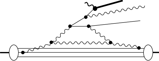
FIG. 1.: A graph for $e+p\to p+X$.

The model of Ingelman and Schlein [2] as applied to deeply inelastic scattering is simple to state. We begin with the usual factorization theorem for the structure function $F_{2}$:

$$F_{2}(x,Q^{2})=\sum_{a}\int_{0}^{1}d\xi\ f_{a/A}(\xi,\mu)\ \hat{F}_{2,a}(x/\xi,Q^{2};\mu).$$ (5)

Here $f_{a/A}(\xi,\mu)$ is the distribution of partons of kind $a$ in hadron $A$ as a function of momentum fraction $\xi$, as measured at a factorization scale $\mu$, while $\hat{F}_{2,a}$ is the structure function for deeply inelastic scattering on parton $a$. If, for simplicity, we ignore $Z$ exchange, then $\hat{F}_{2}$ is

$$\hat{F}_{2,a}(x/\xi,Q^{2};\mu)=e_{a}^{2}\ \delta(1-x/\xi)+{\cal O}(\alpha_{s}).$$ (6)

Thus $F_{2}$ is rather trivially related to the parton distribution functions at the Born level; nevertheless, conceptually the distinction between $F_{2}(x,Q^{2})$ and $f_{a/A}(\xi,\mu)$ is quite important. As in our previous paper [5], we break the analysis into two stages. In the first stage, we hypothesize that the diffractive structure function $F_{2}^{\rm diff}$ can be written in terms of a diffractive parton distribution, Eq. (2):

$${dF_{2}^{\rm diff}(x,Q^{2};x_{IP},t)\over dx_{IP}\,dt}=\sum_{a}\int_{0}^{x_{IP}}d\xi\ {d\,f^{\rm diff}_{a/A}(\xi,\mu;x_{IP},t)\over dx_{IP}\,dt}\ \hat{F}_{2,a}(x/\xi,Q^{2};\mu).$$ (7)

In the second stage, we hypothesize that ${d\,f^{\rm diff}_{a/A}(x_{a},\mu)/dx_{IP}\,dt}$ has a particular form:

$${d\,f^{\rm diff}_{a/A}(\xi,\mu;x_{IP},t)\over dx_{IP}\,dt}={1\over 8\pi^{2}}\,|\beta_{A}(t)|^{2}x_{IP}^{-2\alpha(t)}\,f_{a/{IP}}(\xi/x_{IP},t,\mu)\,.$$ (8)

Here $\beta_{A}(t)$ is the pomeron coupling to hadron A and $\alpha(t)$ is the pomeron trajectory. We distinguish the “Regge factorization” of Eq. (8) from the “diffractive factorization” of Eq. (7).

In Eq. (8) we adopt standard conventions such that the proton-proton elastic scattering amplitude is

$${\cal M}=-\beta_{p}(t)^{2}s^{\alpha(t)}\,.$$ (9)

Then the elastic scattering cross section is

$${d\sigma\over dt}={1\over 16\pi}|\beta_{p}(t)|^{4}s^{2(\alpha(t)-1)}\,.$$ (10)

while the total proton-proton cross section is

$$\sigma_{\rm tot}(pp)=\Re[\beta_{p}(0)^{2}]\,s^{\alpha(0)-1}\,.$$ (11)

The normalization factor $1/(8\pi^{2})$ in Eq. (8) is quite arbitrary. Here, we have adopted the convention of Donnachie and Landshoff [7].

The function $f_{a/{IP}}(\beta,t,\mu)$ thus defined is the “distribution of partons in the pomeron.” In writing Eq. (8), one thinks of the pomeron as a continuation in the angular momentum plane of a set of hadron states. Since hadrons contain partons, the pomeron should also. Thus one has in Eq. (8) the standard factors describing the coupling of the pomeron to hadron A, together with a distribution of partons in the pomeron [2, 3]. Inserting Eq. (8) into (7), one obtains the model of Ingelman and Schlein, applied to the case of deeply inelastic scattering:

$${dF_{2}^{\rm diff}(x,Q^{2};x_{IP},t)\over dx_{IP}\,dt}={|\beta_{A}(t)|^{2}\over 8\pi^{2}}\,x_{IP}^{1-2\alpha(t)}\,\sum_{a}\int_{0}^{1}d\tilde{\beta}\,f_{a/{IP}}(\tilde{\beta},t,\mu)\,\hat{F}_{2,a}(\beta/\tilde{\beta},Q^{2};\mu),$$ (12)

where $\beta=x/x_{IP}$. We offer here a word of caution. Both the structure of Eq. (12) and the language “distribution of partons in the pomeron” suggest that the hadron emits a pomeron some long time before the hard interaction and that the pomeron then splits into partons, one of which participates in the hard interaction. This interpretation is, however, not required by Eq. (12) and is surely quite misleading. In a diagrammatic interpretation of pomeron exchange [8], the exchanged quanta have small plus and minus components of momentum. Thus the exchange takes place over a long interval $(\Delta x^{+},\Delta x^{-})$ in space-time. It begins long before the hard interaction and ends long afterwards. Our diagrammatic analysis in Secs. VII and VIII will provide an illustration of this picture.

We see that Eq. (7), can be regarded as a version of the Ingelman-Schlein model (12) that is more parsimonious in its assumptions. Eq. (7) says only that factorization still applies when hadron $A$ is diffractively scattered. The Ingelman-Schlein model (12) assumes that Regge phenomenology is applicable and, with the aid of this assumption, has more predictive power.

In this paper, we concentrate on the case in which hadron $A^{\prime}$ is the same kind of hadron as hadron $A$, so that vacuum quantum numbers are exchanged, and we consider $x_{IP}$ to be small enough so that pomeron exchange dominates. One should keep in mind, however, that Eq. (7) admits generalizations to cases where $A^{\prime}\neq A$ and where $x_{IP}$ is not at all small. One can also generalize Eq. (12) to $A^{\prime}\neq A$, but then $x_{IP}$ should be fairly small in order that just one or two Regge exchanges dominate.

The diffractive factorization equation (7), or rather a very closely related equation, has been introduced by Veneziano and Trentadue [6]. These authors call the analogue of ${d\,f^{\rm diff}_{a/A}(\xi,\mu)/dx_{IP}\,dt}$ a “fracture function.” Stated precisely, a fracture function is

$${d\,f^{\rm diff}_{a/A}(\xi,\mu;x_{IP})\over dx_{IP}}=\int_{0}^{\infty}d|t|\ {d\,f^{\rm diff}_{a/A}(\xi,\mu;x_{IP},t)\over dx_{IP}\,dt}.$$ (13)

By integrating over $t$, Veneziano and Trentadue eliminate a variable that is perhaps of secondary importance. However, there is some advantage to not integrating over $t$. We are interested in the physics of diffraction, which occurs in the small $t$ region. If we integrate over $t$, then we are forced to consider also the large $t$ region, in which the hadron $A^{\prime}$ is to be thought of not as the original hadron appearing in a scattered form but as a random hadron in a high $P_{T}$ jet produced in the hard interaction. Taking this possibility into account leads to certain complications in the formulas.

In the following sections, we analyze the diffractive parton distributions. According to Eq. (7), the measured quantity $dF_{2}^{\rm diff}/dx_{IP}\,dt$ is approximately the sum of diffractive quark distributions weighted by the square of the quark charges. There are higher order corrections to this relation, some involving the diffractive gluon distribution. Thus these distributions are rather directly related to experiment. The reader may wonder why we concentrate on the theoretical diffractive parton distributions rather than on the physical quantity $dF_{2}^{\rm diff}/dx_{IP}\,dt$. The reasons are the same as in ordinary hard scattering: 1) the diffractive parton distributions are process independent and 2) the factorization (7) allows one to include perturbative corrections to the hard scattering. The reader may also wonder why we don’t frame the analysis in terms of the distribution of partons in the pomeron. Our excuse is ignorance. We don’t know how to relate the Regge factorization in Eq. (8) to quantum field theory.

III The diffractive parton distribution

In this section we give an operator definition of the diffractive parton distribution. We write the ordinary distribution of a quark of type $j\in\{u,\bar{u},d,\bar{d},\dots\}$ in a hadron of type $A$ in terms of field operators $\tilde{\psi}(y^{+},y^{-},{\bf y})$ evaluated at $y^{+}=0$, ${\bf y}=0$ [9, 10]:

$$f_{j/A}(\xi,\mu) \equiv \!{1\over 4\pi}{1\over 2}\sum_{s_{\!A}}\!\int\!dy^{-}e^{-i\xi P_{\!A}^{+}y^{-}}\langle P_{\!A},s_{\!A}|\tilde{\overline{\psi}}_{j}(0,y^{-},{\bf 0})\gamma^{+}\tilde{\psi}_{j}(0)|P_{\!A},s_{\!A}\rangle.$$ (14)

Similarly, the ordinary distribution of a gluon in a proton is written as

$$f_{g/A}(\xi,\mu) \equiv \!{1\over 2\pi\xi P_{\!A}^{+}}{1\over 2}\sum_{s_{\!A}}\!\int\!dy^{-}e^{-i\xi P_{\!A}^{+}y^{-}}\langle P_{\!A},s_{\!A}|\tilde{F}_{a}^{\dagger}(0,y^{-},{\bf 0})^{+\nu}\tilde{F}_{a}(0)_{\nu}^{\ +}|P_{\!A},s_{\!A}\rangle.\ \$$ (15)

The proton state $|P_{\!A},s_{\!A}\rangle$ has spin $s_{\!A}$ and momentum $P_{\!A}^{\mu}=(P_{\!A}^{+},{M_{\!A}^{2}/[2P_{\!A}^{+}]},{\bf 0})$. We average over the spin. Our states are normalized to

$$\langle k|p\rangle=(2\pi)^{3}\,2p^{0}\,\delta^{3}(\vec{p}-\vec{k})=(2\pi)^{3}\,2p^{+}\,\delta(p^{+}-k^{+})\,\delta^{2}({\bf p}-{\bf k})$$ (16)

The field $\tilde{\psi}_{j}(0,y^{-},{\bf 0})$ is the quark field operator modified by multiplication by an exponential of a line integral of the vector potential:

$$\tilde{\psi}_{j}(0,y^{-},{\bf 0})=\left[{\cal P}\exp\left(ig\int_{y^{-}}^{\infty}dx^{-}\,A_{c}^{+}(0,x^{-},{\bf 0})\,t_{c}\right)\right]\psi_{j}(0,y^{-},{\bf 0})\,.$$ (17)

Likewise $\tilde{F}_{a}(0,y^{-},{\bf 0})^{+\nu}$ is defined by

$$\tilde{F}_{a}(0,y^{-},{\bf 0})^{\mu\nu}=\left[{\cal P}\exp\left(ig\int_{y^{-}}^{\infty}dx^{-}\,A_{c}^{+}(0,x^{-},{\bf 0})\,t_{c}\right)\right]_{ab}F_{b}(0,y^{-},{\bf 0})^{\mu\nu}\,.$$ (18)

The ${\cal P}$ denotes path ordering of the exponential. The matrices $t_{c}$ in Eq. (17) are the generators of the $\bf 3$ representation of SU(3), while in Eq. (18) they are the generators of the $\bf 8$ representation. These operator products are ultraviolet divergent, and are renormalized at scale $\mu$ using the $\overline{\rm MS}$ prescription, as described in [9].

The motivation for these definitions is that in QCD canonically quantized on null surfaces $x^{+}=const.$ using $A^{+}=0$ gauge, the operators measure the probability to find a quark and gluon respectively carrying plus component of momentum equal to $\xi P_{\!A}^{+}$. The line integrals of the color potential restore gauge invariance. Then $\overline{\rm MS}$ renormalization removes divergences.

The line integrals of the color potential have a physical interpretation. Whenever a parton is measured by a short distance probe, the color carried by that parton has to go somewhere. For instance, in deeply inelastic scattering, the color is carried away by the recoiling struck quark. In the definition of the parton distribution function, the recoil color flow is idealized as an infinitely narrow jet moving with the speed of light along the path $x^{\mu}=(0,x^{-},{\bf 0})$ with $y^{-}<x^{-}<\infty$. Any gluons from the color field of the hadron can couple to this idealized color source.

Consider now the diffractive distribution of a quark in a proton. The operator is the same as in Eq. (14), but the proton is required to appear in the final state carrying momentum $P_{\!A}^{\prime}$:

$$(2\pi)^{3}2E_{\!A^{\prime}}\ {d\,f^{\rm diff}_{j/A}(\xi,\mu)\over d^{3}\vec{P}_{\!A^{\prime}}}=G_{j/A}^{\rm diff}(P_{\!A},p_{\!A^{\prime}},\xi,\mu)$$ (19)

$$\equiv {1\over 4\pi}{1\over 2}\sum_{s_{\!A}}\int dy^{-}e^{-i\xi P_{\!A}^{+}y^{-}}\sum_{X,s_{\!A^{\prime}}}\langle P_{\!A},s_{\!A}|\tilde{\overline{\psi}}_{j}(0,y^{-},{\bf 0})|P_{\!A^{\prime}},s_{\!A^{\prime}};X\rangle$$ (21)

$$\hskip 99.58464pt\times\gamma^{+}\langle P_{\!A^{\prime}},s_{\!A^{\prime}};X|{\tilde{\psi}}_{j}(0)|P_{\!A},s_{\!A}\rangle.$$

We sum over the spin $s_{\!A^{\prime}}$ of the final state proton and over the states $X$ of any other particles that may accompany it. Similarly, the diffractive distribution of gluons in a hadron is

$$(2\pi)^{3}2E_{\!A^{\prime}}\ {d\,f^{\rm diff}_{g/A}(\xi,\mu)\over d^{3}\vec{P}_{\!A^{\prime}}}=G_{g/A}^{\rm diff}(P_{\!A},P_{\!A^{\prime}},\xi,\mu)$$ (22)

$$\equiv {1\over 2\pi\xi P_{\!A}^{+}}{1\over 2}\sum_{s_{\!A}}\int dy^{-}e^{-i\xi P_{\!A}^{+}y^{-}}\sum_{X,s_{\!A^{\prime}}}\langle P_{\!A},s_{\!A}|\tilde{F}_{a}(0,y^{-},{\bf 0})^{+\nu}|P_{\!A^{\prime}},s_{\!A^{\prime}};X\rangle$$ (24)

$$\hskip 113.81102pt\times\langle P_{\!A^{\prime}},s_{\!A^{\prime}};X|\tilde{F}_{a}(0)_{\nu}^{\ +}|P_{\!A},s_{\!A}\rangle.$$

The Green function $G_{a/A}^{\rm diff}$ for a parton of type $a$ can, at least in principle, be computed from Feynman diagrams together with the Bethe-Salpeter wave functions for the bound states.

We will want to change variables to $x_{IP}$ and $t$ as defined in the previous section. Using Eqs. (3) and (4), we obtain

$${d^{3}{\vec{P}_{\!A^{\prime}}}\over 2E_{\!A^{\prime}}}={dx_{IP}\over 2(1-x_{IP})}\ d^{2}{\bf P}_{\!A^{\prime}}={1\over 4}\,dx_{IP}\,dt\,d\phi\,.$$ (25)

Integrating over the azimuthal angle $\phi$, we have

$${d\,f^{\rm diff}_{a/A}(\xi,\mu)\over dx_{IP}\,dt}={1\over 16\pi^{2}}\ G_{a/A}^{\rm diff}(P_{\!A},P_{\!A^{\prime}},\xi,\mu)$$ (26)

where $G_{j/A}^{\rm diff}$ for quarks is given in Eq. (21) and $G_{g/A}^{\rm diff}$ for gluons is given in Eq. (24).

IV Evolution equation

As mentioned in the previous section, the diffractive parton distributions are ultraviolet divergent and require renormalization. It is convenient to perform the renormalization using the $\overline{\rm MS}$ prescription, as discussed in [9, 10]. This introduces a renormalization scale $\mu$ into the functions. In applications, one sets $\mu$ to be the same order of magnitude as the hard scale of the physical process.

The renormalization involves ultraviolet divergent subgraphs, such as that shown in Fig. 2(a). Subgraphs with more than two external parton legs carrying physical polarization, such as that shown in Fig. 2(b), do not have an overall divergence. Thus the divergent subgraphs are the same as for the ordinary parton distributions. We conclude that the renormalization group equation for the diffractive parton distributions is

$$\mu{d\over d\mu}\,{df^{\rm diff}_{a/A}(\xi,\mu;x_{IP},t)\over dx_{IP}\,dt}=\sum_{b}\int_{\xi}^{1}{dz\over z}\ P_{a/b}(\xi/z,\alpha_{s}(\mu))\ {df^{\rm diff}_{b/A}(z,\mu;x_{IP},t)\over dx_{IP}\,dt}$$ (27)

with the same DGLAP kernel [11], $P_{a/b}(\xi/z,\alpha_{s}(\mu))$, as one uses for the evolution of ordinary parton distribution functions.

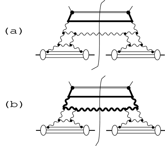
FIG. 2.: Renormalization of the diffractive quark distribution. The subgraph in (a) denoted by heavy lines is ultraviolet divergent, and thus contributes to the evolution kernel. The subgraph in (b) is not ultraviolet divergent (with transverse polarizations for the incoming gluons). The diagrammatic notation is that of Ref. [9]

.

If, following Veneziano and Trentadue, we integrate over $t$, then the large $t$ integration region introduces new ultraviolet divergences and the renormalization group equation is modified [6]. In this paper, we choose to restrict integrations over $t$ to the small $t$ region.

V Validity of diffractive factorization

In Sec. II, we presented the hypothesis of diffractive factorization for diffractive deeply inelastic scattering, as represented by Eq. (7):

$${dF_{2}^{\rm diff}(x,Q^{2};x_{IP},t)\over dx_{IP}\,dt}\sim\sum_{a}\int_{0}^{1}d\xi\ {d\,f^{\rm diff}_{a/A}(\xi,\mu;x_{IP},t)\over dx_{IP}\,dt}\ \hat{F}_{2,a}(x/\xi,Q^{2};\mu).$$ (28)

This is an example of the more general hypothesis of factorization for other kinds of diffractive hard scattering. Another example is diffractive jet production. Consider, for example, the inclusive cross section for the production of two jets in a high energy collisions of two hadrons, $A$ and $B$. (At HERA, this would be $p+\gamma\to jets$ where hadron $B$ is the the hadronic or “resolved” part of the photon.) Let the initial hadron $A$ have momentum

$$P_{\!A}^{\mu}=(P_{\!A}^{+},P_{\!A}^{-},{\bf P}_{\!A})=(P_{\!A}^{+},{M^{2}\over 2P_{\!A}^{+}},{\bf 0})\,,$$ (29)

while hadron $B$ enters the scattering with momentum

$$P_{\!B}^{\mu}=(P_{\!B}^{+},P_{\!B}^{-},{\bf P}_{\!B})=({M^{2}\over 2P_{\!B}^{-}},P_{\!B}^{-},{\bf 0})\,.$$ (30)

We specify the two jets by variables $E_{T}$, $X_{A}$, and $X_{B}$, given in terms of the four momenta $P_{\!1}^{\mu}$ and $P_{\!2}^{\mu}$ of jets $1$ and $2$ by

$$E_{T} = (|{\bf P}_{\!1}|+|{\bf P}_{\!2}|)\,,$$ (31)

$$X_{A} = (P_{\!1}^{+}+P_{\!2}^{+})/P_{\!A}^{+}\,,$$ (32)

$$X_{B} = (P_{\!1}^{-}+P_{\!2}^{-})/P_{\!B}^{-}\,.$$ (33)

If we add the requirement that hadron $A$ emerge scattered with scattering parameters $(x_{IP},t)$, then we have diffractive jet production. The corresponding hypothesis of diffractive factorization for this cross section is

$${d\sigma^{\rm diff}(A+B\to A+{\rm jets}+X)\over dE_{T}\,dX_{A}\,dX_{B}\,dx_{IP}\,dt}\sim$$ (35)

$$\sum_{a,b}\int dx_{a}\,{d\,f^{\rm diff}_{a/A}(x_{a},\mu;x_{IP},t)\over dx_{IP}\,dt}\int dx_{b}\,f_{b/B}(x_{b},\mu)\ {d\hat{\sigma}(a+b\to{\rm jets}+X)\over dE_{T}\,dX_{A}\,dX_{B}}\,.$$

Of course, Eqs. (28) and (35) are approximations, as indicated by the $\sim$ signs. We understand the hypothesis of diffractive factorization to mean that the corrections to these relations are suppressed by a power of $m/Q$ or $m/E_{T}$, where $m$ represents the momentum scale of soft hadronic interactions and $Q$ or $E_{T}$ is the scale of the hard interaction.

This general diffractive factorization hypothesis was put forward by Veneziano and Trentadue in their paper [6] on fracture functions. The Ingelman-Schlein model [2] demands diffractive factorization plus the Regge structure of the diffractive parton distributions. Thus, in a strict interpretation, the validity of the Ingelman-Schlein model logically implies the validity of diffractive factorization. On the other hand, one might interpret the Ingelman-Schlein model as being valid if corrections to it, while not vanishing in the limit of large $Q$, were nevertheless numerically small. Thus, for instance, the authors of Ref. [3] speculated that the factorization inherent in the Ingelman-Schlein model was not likely to be exact up to $m/Q$ corrections but might have the same status as Regge factorization, which has proven to be a useful approximation even if it is not exact.

The hypothesis of diffractive factorization appears to us to be correct in the case of deeply inelastic scattering. A detailed proof of this statement is beyond the scope of this paper. However, we can briefly sketch how such a proof would go, following the ideas of Refs. [12, 13]. The singularities of the cut Feynman graphs for diffractive deeply inelastic scattering are such that the leading integration regions involve 1) a beam jet in the direction of the initial hadron $A$ (which includes the final state diffracted hadron $A^{\prime}$), 2) a hard interaction, 3) one or more final state jets that are not in the direction of hadron $A$, and 4) possible soft gluons (sometimes with soft quark loops) that may communicate between the beam jet and the final state jets. Factorization would be more or less kinematic were it not for the possibility of the soft gluons linking the beam jet with the final state jets. One must use gauge invariance to show that the soft gluons don’t really “see” the details of the final state jets, so that the connections to the final state jets can be replaced by connections to the idealized jet that is embodied in the line integral of the field operator $A_{\mu}$ in the definitions of the diffractive parton distribution functions, Eqs. (14,15,17,18).

What of diffractive factorization for processes with two hadrons in the initial state, such as $\bar{p}+p\to jets$ or $\gamma+p\to jets$? Here the proof of ordinary factorization is much more delicate. The problem is that low momentum gluons can communicate between the partons of the two beam jets. This can happen even before the hard scattering takes place, as in Fig. 3. When one looks for the hard process inclusively, such effects cancel [12, 13]. But the cancellation requires a sum over final states. Collins, Frankfurt, and Strikman [14] have argued that the demand that the final state include a diffractively scattered hadron destroys the factorization. In Ref. [5], we looked at this problem in the context of a simple perturbative model. We found that the diffractive factorization hypothesis is, indeed, not valid. New terms proportional to $\delta(1-X_{A}/x_{IP})$ appear in Eq. (35). (Presumably in a more general model one will also have factorization violating terms that are not proportional to $\delta(1-X_{A}/x_{IP})$ but are singular as $(1-X_{A}/x_{IP})\to 0$.) These new terms have an interesting structure that can be investigated experimentally at HERA.

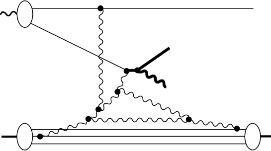
FIG. 3.: A graph for $\gamma+p\to p+{\rm jets}+X$ for which diffractive factorization fails because of soft color interactions among the spectator partons.

VI Diffractive parton distributions for $\beta\to 0$

The diffractive parton distribution ${d\,f^{\rm diff}_{a/A}(\xi,\mu;x_{IP},t)/dx_{IP}\,dt}$ is essentially a long distance object, which is not amenable to calculation using perturbative methods. However, Regge phenomenology provides an expectation for the behavior of ${d\,f^{\rm diff}_{a/A}(\xi,\mu;x_{IP},t)/dx_{IP}\,dt}$ when the parameter

$$\beta=\xi/x_{IP}$$ (36)

is small compared to 1. In the case of the ordinary parton distributions, this expectation is

$$f_{a/A}(x,\mu)\sim{\rm const.}\times(1/x)^{\tilde{\alpha}(0)}$$ (37)

where $\tilde{\alpha}(0)$ is the pomeron intercept. That is, one expected

$$F_{2}(x,Q^{2})\sim{\rm const.}\times(1/x)^{\tilde{\alpha}(0)-1}$$ (38)

for small $x$. The simplest version of this expectation is that $\tilde{\alpha}(0)$ is the same as in soft pomeron physics, $\alpha(0)-1\approx 0.08$ [15]. However, this expectation is hard to reconcile with evolution: if it holds at some rather small value of $Q^{2}$, then $F_{2}$ should be steeper at larger values of $Q^{2}$ [16]. A steeper dependence was also expected on the basis of the perturbative version of the pomeron analyzed at leading log level [17]. Indeed, a steeper dependence, with $\tilde{\alpha}(0)-1\approx 0.4$, is found in experiments at HERA [18].

The analogous expectation [3] for the $\beta$ dependence of diffractive parton distributions at fixed $x_{IP}$ is

$${d\,f^{\rm diff}_{a/A}(\beta x_{IP},\mu;x_{IP},t)\over dx_{IP}\,dt}\sim{\rm const.}\times\left(1\over\beta\right)^{\tilde{\alpha}(0)}.$$ (39)

In this case, the constant is proportional to the triple pomeron coupling used in Regge physics. Presumably, $\tilde{\alpha}(0)$ here should not be the true pomeron intercept $\approx 1.08$ but should be the larger value, $\approx 1.4$, found in the HERA experiments. Then, of course, it is debatable whether the triple pomeron coupling used here should be the same as that found in soft Regge physics. Uncertainty over the precise values, however, should not obscure the simple prediction that the diffractive $F_{2}$ should behave at small $\beta$ like

$${d\,F_{2}^{\rm diff}(\beta x_{IP},Q^{2};x_{IP},t)\over dx_{IP}\,dt}\sim{\rm const.}\times\left(1\over\beta\right)^{\tilde{\alpha}(0)-1}.$$ (40)

with $0\lesssim\tilde{\alpha}(0)-1\lesssim 0.5$. The small $\beta$ behavior of $F_{2}^{\rm diff}$ is analyzed in Refs. [19].

VII Gluon distribution for $\beta\to 1$

The diffractive parton distribution ${d\,f^{\rm diff}_{a/A}(\xi,\mu;x_{IP},t)/dx_{IP}\,dt}$, like the ordinary parton distribution, is essentially not calculable using perturbative methods. Recall, however, that it is possible to derive “constituent counting rules” that give predictions for ordinary parton distributions ${f_{a/A}(x,\mu)}$ in the limit $x\to 1$ for not too large values of the scale parameter $\mu$ [20]. In the same spirit, we consider in this section and the next the diffractive parton distributions in the limit $\beta\to 1$ where $\beta=\xi/x_{IP}$. Our analysis is similar to that if Ref. [3]. The authors of that paper concluded, with certain caveats, that the diffractive gluon distribution should behave like $(1-\beta)^{1}$ as $\beta\to 1$. Our reanalysis suggests a behavior between $(1-\beta)^{1}$ and $(1-\beta)^{0}$, depending on how certain nonperturbative issues are resolved. For the diffractive quark distribution (not treated in Ref. [3]), our analysis in Sec. VIII suggests a behavior between $(1-\beta)^{2}$ and $(1-\beta)^{1}$.

This analysis involves both hard and soft subprocesses, put together in a manner that is not under solid theoretical control. Thus there is not a clearly correct final answer, as far as we can see. What we do here is to provide some calculational results that can help restrict the range of answers and give some basis for the reader’s informed judgment.

Define $\tau=\beta-1=\xi/x_{IP}-1$. Then we examine ${d\,f^{\rm diff}_{a/A}((1-\tau)x_{IP},\mu;x_{IP},t)/dx_{IP}\,dt}$ in the limit $\tau\to 0$, after first taking $x_{IP}<<1$ so as to separate out pomeron exchange from other Regge pole exchanges. We consider the diffractive gluon distribution first (a = g). Later, we supply the modifications needed for the diffractive quark distribution. Throughout this section, except as specifically noted, we consider Feynman graphs in null plane gauge $A^{+}=0$.

Our analysis is based on a model that consists of a selected set of Feynman graphs, with the internal loop momenta integrated over a selected integration region. Within this model there is a hard subgraph in which all internal propagators are far off-shell and a soft subgraph in which the propagators are near to being on-shell. We evaluate the hard subgraph at lowest order in perturbation theory. We offer a perturbatively based conjecture about the behavior of the soft subgraph in the Regge limit $x_{IP}\to 0$.

The simple graphs considered here do not include the graphs that contribute to QCD evolution of the parton distributions. Thus we imagine that the analysis applies to the diffractive parton distribution at a starting scale $\mu_{0}$ that is not too large (say, 2 GeV). Standard parton evolution starting at this scale will soften the distributions.

A Decomposition into hard and soft subgraphs

According to Eq. (24), the diffractive gluon distribution is the square of the matrix element of an operator that destroys a gluon with longitudinal momentum fraction $(1-\tau)x_{IP}$, where the matrix element is taken between the initial proton state and a final state that includes the scattered hadron plus anything else. Since a color octet gluon is destroyed, while the initial and final hadrons are color singlets, the final state must include at least one gluon. We consider here the minimal model in which the final state includes precisely one gluon. Then this gluon carries a very small momentum fraction $\tau x_{IP}$. Call the momentum of the final state gluon $q^{\mu}$, as depicted in Fig. 4. Since this gluon is on-shell, we have

$$q^{\mu}=(\tau x_{IP}P_{\!A}^{+},{{{\bf q}^{2}}\over{2\tau x_{IP}P_{\!A}^{+}}},{\bf q}).$$ (41)

Before proceeding, we pause for a technical point. In general in this section we use the null plane gauge $A^{+}=0$, but for the final state gluon this is not convenient. The polarization vectors $\epsilon^{\mu}(q,j)$ for transverse polarization in the $j$ direction have minus components that grow like $1/\tau$ in the limit $\tau\to 0$:

$$\epsilon^{-}(q,j)={q^{j}\over q^{+}}={q^{j}\over x_{IP}\tau P_{\!A}^{+}}.$$ (42)

We avoid this singular behavior by changing the polarization vectors for this gluon to $A^{-}=0$ gauge. The difference $\Delta\epsilon^{\mu}$ between the old polarization vector and the new is proportional to $q^{\mu}$, so that changing polarization vectors has no effect after we sum over a gauge invariant set of graphs. In $A^{-}=0$ gauge, $\epsilon^{-}(q,j)=0$, $\epsilon^{i}(q,j)=\delta^{ij}$ and

$$\epsilon^{+}(q,j)={q^{j}\over q^{-}}=x_{IP}\tau P_{\!A}^{+}\,{q^{j}\over{\bf q}^{2}}.$$ (43)

Thus $\epsilon^{\mu}(q,j)$ is predominantly transverse, with a plus component that vanishes as $\tau\to 0$.

Some vocabulary will be helpful for discussing the physics of time and momentum scales in this problem. There are three relevant longitudinal momentum scales. We call partons with $p^{+}\sim P_{\!A}^{+}$ fast partons. For instance, the valence quarks in a hadron are typically fast partons. We call partons with $p^{+}\sim x_{IP}P_{\!A}^{+}$ slow partons. Finally, we call partons with $p^{+}\sim\tau x_{IP}P_{\!A}^{+}$ very slow partons. The final state gluon is such a parton.

The gluon cloud surrounding any hadron contains gluons at any momentum fraction. Consider a gluon with momentum fraction $x$ and transverse momentum of order $m$, where $m\approx 0.3\ {\rm GeV}$ gives the scale of a typical hadronic mass or transverse momentum. The contribution of such a gluon to the null plane energy $P^{-}$ of an intermediate state is $p^{-}={\bf p}^{2}/2p^{+}$, which is the minus momentum of a free gluon with transverse momentum ${\bf p}$ and plus momentum $p^{+}$. This “kinetic” minus momentum is of order $m^{2}/(xP_{\!A}^{+})$. Thus a gluon of the type that we are calling a slow gluon has a kinetic null plane energy $p^{-}\sim m^{2}/(x_{IP}P_{\!A}^{+})$ and survives for a typical null plane time $\Delta z^{+}\sim xP_{\!A}^{+}/m^{2}$.

Notice that the final state gluon has a large minus momentum, $q^{-}={{{\bf q}^{2}}/({2\tau x_{IP}P_{\!A}^{+}})}$, at least as long as its transverse momentum $\bf q$ is not too small. Now $\bf q$ is not observed; we are to square the matrix element and integrate over $\bf q$. We cannot say anything about the region of very small $\bf q$, but we can analyze the contribution to the integral from the region $\cal R$ defined by

$${\bf q}^{2}\gg\tau m^{2}.$$ (44)

We will consider the contribution to $df^{\rm diff}/dx_{IP}\,dt$ from the region $\cal R$ with the hope that the contribution from the complementary region ${\bf q}^{2}\lesssim\tau m^{2}$, is not large enough to overwhelm — or, worse, to cancel — the contribution from region $\cal R$.

We will also evaluate the contribution from the smaller integration region in which the transverse momentum ${\bf q}$ is large: ${\bf q}^{2}\gg m^{2}$. Since this region is described by rather standard short distance dynamics, its contribution should provide a lower bound on the true result. (Again, we assume that this contribution is not canceled by some long distance contribution.)

For ${\bf q}\in{\cal R}$ the minus momentum $q^{-}={{{\bf q}^{2}}/({2\tau x_{IP}P_{\!A}^{+}})}$ of the final state gluon is large compared to the kinetic minus momentum $p^{-}\sim m^{2}/P_{\!A}^{+}$ of a typical fast parton and is also large compared to the kinetic minus momentum $p^{-}\sim m^{2}/(x_{IP}P_{\!A}^{+})$ of a typical slow parton. This large minus momentum flows through the graph and is carried out of the graph by the detected gluon. Thus the parton detection with $\tau\to 0$ creates a hard process that happens on a null plane time scale $\Delta x^{+}$ that is short compared to the typical time scale for interactions within the proton or its cloud of slow gluons. We base our analysis on this observation, using low order perturbation theory for the nearly instantaneous interaction that probes the parton distribution.

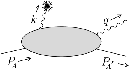
FIG. 4.: Structure of amplitude contributing to the diffractive gluon distribution. At least one gluon must be emitted into the final state.

Three graphs that involve the lowest order hard interaction are shown in Fig. 5. In these graphs, the large minus momentum $q^{-}$ flows through only one or two propagators, as indicated by the heavy lines. These propagators are far off shell. We refer to this part of the graph as the hard subgraph. The rest of the graph is the soft subgraph.

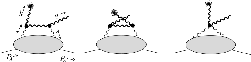
FIG. 5.: Graphs with an order $g^{2}$ hard subgraph.

There are also two graphs of the same order that involve connecting the $q^{\mu}$ and $k^{\mu}$ gluons to a quark line, as depicted in Fig. 6. These graphs require a separate discussion, which we omit in this paper on the grounds that low momentum gluons are likely to be dominant in the pomeron compared to low momentum quarks.

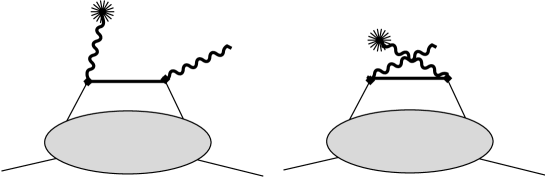
FIG. 6.: More graphs with an order $g^{2}$ hard subgraph. These graphs involve quark exchange from the soft subgraph and are not considered in this paper.

In Fig. 5, we denote by $r^{\mu}$ and $s^{\mu}$, respectively, the momenta of the gluon leaving the soft subgraph and entering it after the hard interaction. Let the momentum fraction of the first gluon be $r^{+}/P_{\!A}^{+}=(1+\sigma)x_{IP}$. Then momentum conservation fixes $s^{+}/P^{+}=\sigma x_{IP}$.

We integrate over $\sigma$. It is convenient to distinguish between the two identical gluons by requiring that $r^{+}>-s^{+}$. That is, $\sigma>-1/2$. In principle, the $\sigma$ integration runs to $\sigma=\infty$, but the reader can verify that the region $\sigma\gg 1$ is not important. We take it as a working assumption, to be verified later, that the region $|\sigma|\ll 1$ is also not important. Thus the important integration region is $\sigma\sim 1$. That is, the gluons that couple the hard subgraph to the soft subgraph are typical “slow” gluons.

We integrate over the transverse momentum ${\bf r}$, setting ${\bf s}={\bf r}+{\bf l}$. We also integrate over $r^{-}$, setting $s^{-}=r^{-}-M_{\!A}^{2}/(2P_{\!A}^{+})+(M_{\!A}^{2}+({\bf P}_{\!A^{\prime}})^{2})/(2(1-x_{IP})P_{\!A}^{+})$. We suppose that the hadron wave functions fix ${\bf r}$ and $r^{-}$ to be no larger than the ordinary size for slow gluons, ${\bf r}^{2}\sim m^{2}$ and $r^{-}\lesssim m^{2}/(x_{IP}P_{\!A}^{+})$. (Contributions in which $r^{\mu}$ is part of a hard virtual loop are more properly considered to be part of a higher order correction to the hard subgraph.)

Taking the limit $\tau\to 0$, we find that if we consider the hard subgraph to be a function of $r^{\mu}$, $s^{\mu}$, and $q^{\mu}$, then it is independent of $r^{-}$, $s^{-}$, ${\bf r}$ and ${\bf s}$ and is also also independent of $x_{IP}$. In addition, the dominant polarizations for the gluons entering the hard subgraph from the soft subgraph are transverse; in a shorthand notation,

$$\sum_{\mu,\nu=\{+,-,1,2\}}[{\rm Hard}]^{\mu\nu}[{\rm Soft}]_{\mu\nu}\approx\sum_{i,j=\{1,2\}}[{\rm Hard}]^{ij}[{\rm Soft}]_{ij}.$$ (45)

That the hard subgraph is independent of $r^{-}$ and $s^{-}$ is not surprising, since $r^{-}\ll q^{-}$ and $s^{-}\ll q^{-}$. That it is independent of $x_{IP}$ follows simply from its invariance under boosts in the longitudinal direction. It is not, however, obvious that the hard subgraph is independent of ${\bf r}$ and ${\bf s}$ and that only transverse polarizations are important. These results follow from an argument that we describe in Appendix A. The picture that emerges is one in which the soft gluon cloud surrounding the hadron is probed by an interaction that is effectively local in null plane time, $x^{+}$ and in transverse position $\bf x$.

B Structure of the diffractive gluon distribution

We take advantage of these results by setting $r^{-}=s^{-}=0$ and ${\bf r}={\bf s}={\bf 0}$ in the hard subgraph and restricting the polarization sum to transverse polarizations. Then the diffractive distribution function depends on the integral over $r^{-}$ and ${\bf r}$ of the soft subgraph. We write this structure as depicted in Fig. 7,

$${{df_{g/A}^{\rm diff}}\over{dx_{IP}\,dt}} = {1\over{64\pi^{3}\tau}}\,{1\over 2}\sum_{s_{\!A},s_{\!A^{\prime}}}\,\sum_{ijkl}\int_{-1/2}^{\infty}d\sigma^{\prime}A_{kl}^{*}(\sigma^{\prime},x_{IP},t;s_{\!A},s_{\!A^{\prime}})\int_{-1/2}^{\infty}d\sigma A_{ij}(\sigma,x_{IP},t;s_{\!A},s_{\!A^{\prime}})$$ (47)

$$\times\sum_{mnab}\int_{\cal R}{{d^{2}{\bf q}}\over{(2\pi)^{2}}}{{{\cal M}_{ab}^{klmn}({\bf q},\sigma^{\prime},\tau)^{*}\ {\cal M}_{ab}^{ijmn}({\bf q},\sigma,\tau)}\over{(k^{2}-i\epsilon)\ (k^{2}+i\epsilon)}}.$$

Here the first line represents the soft subgraphs while the second line represents the integral of the hard subgraphs. We discuss these factors below.

The function $A_{ij}(\sigma,x_{IP},t;s_{\!A},s_{\!A^{\prime}})$ is the amplitude for the proton to emit a gluon with transverse polarization $i$ and momentum fraction $(1+\sigma)x_{IP}$ then absorb a gluon with transverse polarization $j$ and momentum fraction $\sigma x_{IP}$.

$$A^{ij}(\sigma,x_{IP},t;s_{\!A},s_{\!A^{\prime}}) = x_{IP}P_{\!A}^{+}\sum_{a}\int dy^{-}e^{-i\sigma x_{IP}P_{\!A}^{+}y^{-}}$$ (49)

$$\quad\times\langle P_{\!A^{\prime}},s_{\!A^{\prime}}|{\rm T}\left\{A_{a}^{j}(0,y^{-},0_{T})\,A_{a}^{i}(0)\right\}|P_{\!A},s_{\!A}\rangle.$$

There is a summation over the color $a$ of the gluon operators; in $\cal M$ we average over these colors. The factor $x_{IP}P_{\!A}^{+}$ arises from changing the integration in Eq. (47) from $\int dr^{+}$ to $\int d\sigma$.

We now turn to the hard interaction. We begin by considering the probed gluon, which carries momentum $k^{\mu}$. According to Eqs. (26) and (24), the operator that probes the gluon distribution is $\tilde{F}_{a}^{+m}(y)$. (Only $\nu\in\{1,2\}$ contributes in Eq. (24).) In $A^{+}=0$ gauge, this is simply $\partial^{+}A_{a}^{m}(y)$. (We have changed the polarization vector $\epsilon(q,n)$ for the final state gluon from $\epsilon^{+}=0$, so this gluon could couple to the $A^{+}A^{m}$ operator in $\tilde{F}_{a}^{+m}(y)$. However, this graph is not allowed when the two exchanged gluons are in a color singlet state.) The $\partial^{+}$ becomes a $k^{+}=(1-\tau)x_{IP}P_{\!A}^{+}\sim x_{IP}P_{\!A}^{+}$ that we absorb into the normalization. This leaves a propagator for the probed gluon,

$${-iD^{m\mu}(k)\over k^{2}+i\epsilon}={-i\over k^{2}+i\epsilon}\sum_{j^{\prime}}\epsilon^{m}(k,j^{\prime})\,\epsilon^{\mu}(k,j^{\prime})={-i\over k^{2}+i\epsilon}\,\epsilon^{\mu}(k,m).$$ (50)

Thus each probe operator gives a $1/k^{2}$ factor and leaves the amputated hard interaction graph dotted into a polarization vector for a gluon of momentum $k^{\mu}$, polarization $m$, in $A^{+}=0$ gauge.

We call the amputated hard interaction graph ${\cal M}_{ab}^{ijmn}({\bf q},\sigma,\tau)$. The indices $m$ and $n$ are the transverse polarizations of the probed and final state gluons respectively; $a$ and $b$ are their colors. Recall that the final state gluon polarization is represented by a polarization vector $\epsilon^{\mu}(q,n)$ is, by our convention, in $A^{-}=0$ gauge, as in Eq. (43). In $\cal M$, the exchanged gluons are approximated as having zero transverse and minus momenta; one integrates over these momenta in the definition of $A$. The exchanged gluons have transverse polarizations $i$ and $j$ respectively.

In the $\tau\to 0$ limit, the factor $k^{2}$ in the denominator is

$$k^{2}\sim-{\bf q}^{2}/\tau.$$ (51)

Thus the probed gluon is far off shell, $k^{2}\gg m^{2}$, as long as $\bf q$ is in the integration region $\cal R$, ${\bf q}^{2}\gg\tau m^{2}$. Similarly, the virtual lines internal to $\cal M$ are far off shell and have a simple form when ${\bf q}\in{\cal R}$. This is so even though the region $\cal R$ includes small transverse momenta, ${\bf q}^{2}\ll m^{2}$. Indeed, the small transverse momenta near the boundary of $\cal R$ dominate the integral in Eq. (47), as we will see.

Next, we examine the soft subgraphs and then the hard subgraphs in some detail.

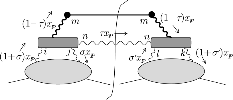
FIG. 7.: Factored structure of the diffractive gluon distribution function for $\tau\to 1$.

C The soft subgraph

In this subsection, we investigate the $x_{IP}$ dependence of $A^{ij}(\sigma,x_{IP},t;s_{\!A},s_{\!A^{\prime}})$ in the limit $x_{IP}\to 0$. Comparing the expected Regge form (8) of ${{df_{g/A}^{\rm diff}}/{dx_{IP}\,dt}}$ with Eq. (47), we see that the expected Regge form of $A^{ij}$ is

$$A^{ij}(\sigma,x_{IP},t;s_{\!A},s_{\!A^{\prime}})\propto x_{IP}^{-\alpha(t)}.$$ (52)

The question is, what is the pomeron trajectory $\alpha(t)$ within the context of the analysis used in this paper?

The operators Eq. (49) are in $A^{+}=0$ gauge, but the amplitude can be put in a gauge invariant form by reexpressing it in terms of the gluon field operators $\tilde{F}^{\mu\nu}$ defined in Eq. (18). We simply replace

$$A^{j}\to{s^{+}A^{j}\over s^{+}+i\epsilon}\to-i{\partial^{+}A^{j}\over s^{+}+i\epsilon}\to-i{\tilde{F}^{+j}\over s^{+}+i\epsilon}$$ (53)

and make a similar replacement for $A^{i}$. The $i\epsilon$ choice here is of some significance. We will discuss it in the following subsection. The resulting form for $A^{ij}$ is

$$A^{ij}(\sigma,x_{IP},t;s_{\!A},s_{\!A^{\prime}}) = {1\over{x_{IP}(\sigma+i\epsilon)(1+\sigma)P_{\!A}^{+}}}\sum_{a}\int dy^{-}e^{-i\sigma x_{IP}P_{\!A}^{+}y^{-}}$$ (55)

$$\quad\times\langle P_{\!A^{\prime}},s_{\!A^{\prime}}|{\rm T}\left\{\tilde{F}_{a}^{+j}(0,y^{-},0_{T})\tilde{F}_{a}^{+i}(0)\right\}|P_{\!A},s_{\!A}\rangle.$$

Since the propagators in the soft subgraph are $\it not$ far off-shell, one is not really justified to use perturbation theory to investigate $A^{ij}(\sigma,x_{IP},t;s_{\!A},s_{\!A^{\prime}})$. Nevertheless, perturbation theory is suggestive. Consider Eq. (55) using Feynman gauge. Suppose that the gluon annihilated by the operator $\tilde{F}_{a}^{+i}$ connects to an on-shell quark carrying no transverse momentum and plus momentum $p^{+}=\lambda P_{\!A}^{+}$, with $\lambda$ of order 1. That is, the gluon couples to a “fast” quark. The relevant factor is

$${-r^{i}\over r^{2}+i\epsilon}\ \bar{\cal U}(\lambda^{\prime}P_{\!A}^{\mu},s)\,igt_{c}\gamma^{+}\,{\cal U}(\lambda P_{\!A}^{\mu},s)\,.$$ (56)

where $\lambda^{\prime}=\lambda-x_{IP}(1+\sigma)$. In the limit $x_{IP}\to 0$, this is independent of $x_{IP}$. Similarly, the coupling of the operator $\tilde{F}_{a}^{+j}$ to a fast quark gives no $x_{IP}$ dependence. Thus perturbation theory suggests that the operator matrix element in Eq. (55) is independent of $x_{IP}$ for small $x_{IP}$. Considering that there is a factor $1/x_{IP}$ in Eq. (55), we find that the pomeron trajectory appearing in Eq. (52) is $\alpha(t)=1$ in this most naive analysis of the soft subgraph. This is close to the pomeron trajectory observed in nature, but of course this most naive analysis is too naive, and we expect that soft interactions among the gluons modify the result. What we see here is that the picture of the pomeron as two gluon exchange, which often gives results that are surprisingly good considering the simplicity of the picture [21], works rather well also in this context.

D Small $\sigma$ singularity

The analysis of the preceding subsection has revealed a $1/\sigma$ singularity within the integration domain $-1/2<\sigma<\infty$ of the momentum fraction $\sigma$. What is the nature of this singularity? If we stick to $A^{+}=0$ gauge, one can check that it arises from the $1/s^{+}$ singularity in the gluon propagator,

$${i\over s^{2}+i\epsilon}\left[-g^{\mu\nu}+{g^{\mu+}s^{\nu}+s^{\mu}g^{\nu+}\over s^{+}}\right].$$ (57)

This singularity is usually interpreted with a principle value prescription, but there is no compelling reason for this choice. In fact, $A^{+}=0$ gauge is not an effective tool for examining the nature of the $1/\sigma$ singularity, since in this gauge the singularity is a gauge artifact. Thus we choose to examine this question in Feynman gauge, in the style of Ref. [12]. (Arguably, it would be better to do the whole problem in Feynman gauge, but this leads to its own complications.)

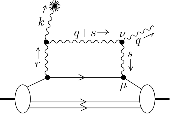
FIG. 8.: Graph with a singularity near $s^{+}=0$.

We consider the graph shown in Fig. 8 in Feynman gauge but with a transverse polarization chosen for the gluon carrying momentum $r^{\mu}$. It is helpful to choose a frame in which $x_{IP}P_{\!A}^{+}\sim m$. Then

$$P_{\!A^{\prime}}^{+}=(1-x_{IP})P_{\!A}^{+}\gg m \quad P_{\!A^{\prime}}^{-}={\bf P}_{\!A^{\prime}}^{2}/[2(1-x_{IP})P_{\!A}^{+}]\ll m$$ (58)

$$q^{+}=\tau x_{IP}P_{\!A}^{+}\ll m \quad q^{-}={\bf q}^{2}/[2\tau x_{IP}P_{\!A}^{+}]\gg m.$$ (59)

The graph contains the structure

$$J^{\mu}\,{-ig_{\mu\nu}\over s^{2}+i\epsilon}\,{N^{\nu}\over(q+s)^{2}+i\epsilon}.$$ (60)

The denominator $(q+s)^{2}$ has the form

$$(q+s)^{2}+i\epsilon=2q\cdot s+s^{2}+i\epsilon=2(q^{-}+s^{-})s^{+}-{\bf q}\cdot{\bf s}+2q^{+}s^{-}-{\bf s}^{2}+i\epsilon$$ (61)

Now $q^{-}$ is large and positive while $s^{-}$ is small in the dominant integration region. Thus the denominator has the approximate form

$${1\over 2q^{-}\,[s^{+}+\cdots+i\epsilon]}$$ (62)

where the dots indicate small terms. This denominator contains the only important dependence on $s^{+}$ as long as $|\sigma|\lesssim 1$ in $s^{+}=\sigma x_{IP}P_{\!A}^{+}$. Notice that there is a singularity very near to $s^{+}=0$, but that, since there are no other singularities nearby, we can deform the integration contour away from this singularity. Thus we deform the $s^{+}$ contour into the upper half complex $s^{+}$ plane. On the deformed contour, we have $s^{+}\sim m$ or $\sigma\sim 1$.

Now we examine the numerators. The largest component of the quark current $J^{\mu}$ is $J^{+}$, while the largest component of the current $N^{\nu}$ of the final state gluon is $N^{-}$. Thus $J_{\mu}N^{\mu}\sim J^{+}N^{-}$. Thus the dominant term in $J_{\mu}N^{\mu}$ is obtained by replacing

$$J_{\mu}N^{\mu}\to{J^{+}\over s^{+}}\ s_{\mu}N^{\mu}.$$ (63)

The factor $s_{\mu}N^{\mu}$ is approximately $s^{+}N^{-}$ as long as $s^{+}$ is not small, and we know that $s^{+}$ is not small since we have deformed the integration contour so that it does not approach $s^{+}=0$.

The next step is to restore the $s^{+}$ integration contour to the real axis, taking care not to cross any singularities. This means that we should move the $1/s^{+}$ singularity in Eq. (63) infinitesimally into the lower half $s^{+}$ plane, so that our replacement becomes

$$J_{\mu}N^{\mu}\to{J^{+}\over s^{+}+i\epsilon}\ s_{\mu}N^{\mu}.$$ (64)

This is in keeping with the usual notation in which integration contours are along the real axis, with poles infinitesimally displaced from the integration contour.

The replacement (64) gives the dominant contribution to our graph. However, if we attach the gluon carrying momentum $s^{\mu}$ everywhere in the hard subgraph and sum the leading terms obtained with this replacement, we will get zero because of the Ward identities obeyed by the hard graph and because the two gluons carrying momenta $r^{\mu}$ and $s^{\mu}$ together form a color singlet. (The relevant identities are discussed in the appendix of Ref. [12]).

We have thus encountered the bête noir of Feynman gauge: the leading contributions graph by graph come from unphysical polarizations that cancel when one sums over graphs. What we need is the subleading contribution. That is easy. We replace

$$J_{\mu}N^{\mu}={J^{+}\over s^{+}+i\epsilon}\ s_{\mu}N^{\mu}+\tilde{J}_{\mu}N^{\mu}.$$ (65)

where

$$\tilde{J}^{\mu}={s^{+}J^{\mu}-J^{+}s^{\mu}\over s^{+}+i\epsilon}.$$ (66)

Now we throw away the first term in (65), since it will cancel, and keep the remainder. This gives the structure in Eq. (53), but now with a prescription for the $1/s^{+}$ singularity determined on physical grounds.

E The hard subgraph

We now turn to the hard interaction function $\cal M$. It is a simple matter to evaluate this function. We find

$${\cal M}_{ab}^{ijmn}({\bf q},\sigma,\tau)=$$ (68)

$${3ig^{2}\over 4(\sigma+i\epsilon)(1+\sigma)}\,\delta_{ab}\biggl{[}\sigma(1+\sigma)\ \delta^{ij}\,\delta^{mn}-\sigma\ \delta^{in}\,\delta^{jm}+(1+\sigma)\ \delta^{im}\,\delta^{jn}\biggr{]}.$$

Thus ${\cal M}\propto\tau^{0}$ as $\tau\to 0$. The $i\epsilon$ prescription in the $1/\sigma$ factor arises from Eq. (62). It matches the $i\epsilon$ prescription in the soft function $A_{ij}$, Eq. (55), so that, after a contour deformation, $\sigma$ is never much smaller than 1.

Inserting Eq. (68) and $k^{2}\sim-{\bf q}^{2}/\tau$ into Eq. (47), we obtain

$${{df_{g/A}^{\rm diff}}\over{dx_{IP}\,dt}} = {1\over{64\pi^{3}\tau}}\,{1\over 2}\sum_{s_{\!A},s_{\!A^{\prime}}}\,\sum_{ijkl}$$ (71)

$$\times\int_{-1/2}^{\infty}d\sigma^{\prime}A_{kl}^{*}(\sigma^{\prime},x_{IP},t;s_{\!A},s_{\!A^{\prime}})\,\int_{-1/2}^{\infty}d\sigma A_{ij}(\sigma,x_{IP},t;s_{\!A},s_{\!A^{\prime}})\ {\cal H}^{klij}(\sigma,\sigma^{\prime})$$

$$\times\int{{d^{2}{\bf q}}\over{(2\pi)^{2}}}{\theta({\bf q}^{2}>\tau M^{2})\over({\bf q}^{2}/\tau)^{2}}.$$

Here ${\cal H}^{klij}(\sigma,\sigma^{\prime})$ is a rational function of $\sigma$ and $\sigma^{\prime}$ that is not of particular interest. Recall that we integrate $\bf q$ over the region $\cal R$ defined by ${\bf q}^{2}\gg\tau m^{2}$ (Eq. (44)), where $m$ is a typical hadronic mass or transverse momentum. Here we make the prescription more precise by integrating over ${\bf q}^{2}>\tau M^{2}$ where $M$ is any fixed mass such that $M\gg m$.

F Result

Performing the integration in Eq. (71) gives for the $\tau\to 0$ limit of the diffractive gluon distribution

$${{df_{g/A}^{\rm diff}}\over{dx_{IP}\,dt}} \sim {1\over{256\pi^{4}\,M^{2}}}\,{1\over 2}\sum_{s_{\!A},s_{\!A^{\prime}}}\,\sum_{ijkl}$$ (73)

$$\times\int_{-1/2}^{\infty}d\sigma^{\prime}A_{kl}^{*}(\sigma^{\prime},x_{IP},t;s_{\!A},s_{\!A^{\prime}})\,\int_{-1/2}^{\infty}d\sigma A_{ij}(\sigma,x_{IP},t;s_{\!A},s_{\!A^{\prime}})\ {\cal H}^{klij}(\sigma,\sigma^{\prime}).$$

Note that ${df_{g/A}^{\rm diff}}/{dx_{IP}\,dt}$ is independent of $\tau$ as $\tau\to 0$:

$${{df_{g/A}^{\rm diff}}(\beta x_{IP},\mu;x_{IP},t)\over{dx_{IP}\,dt}}\sim(1-\beta)^{0}\quad\quad{\rm as}\ \beta\to 1\ {\rm with}\ x_{IP}=const.$$ (74)

This may seem surprising, since the distribution of gluons in a typical hadron behaves like $f_{g/A}(x;\mu_{0})\sim{\rm const.}\times(1-x)^{p}$ with a rather high power $p\approx 5$.

The leading behavior comes from the lower endpoint of the integration in Eq. (71). Thus it is sensitive to the cutoff chosen. Recall that we took ${\bf q}^{2}>\tau M^{2}$ because as long as ${\bf q}^{2}/\tau\gg m^{2}$, the internal lines in the hard subdiagram are far off-shell. This appears to be the natural cutoff. As soon as the internal lines of the subdiagram through which $q^{\mu}$ flows are not far off-shell, the the gluon that goes into the final state and the probed gluon can attach at different space-time points in the gluon cloud of the hadron. Then there is the opportunity for cancellation, as both gluons sample the color charge of the hadron as a whole and find that the hadron as a whole is a color singlet. It is difficult to check this conjecture directly in a realistic model of nonperturbative hadron structure. However we have checked in a very simple model where all the graphs can be included exactly. This model is too simple to have the correct pomeron behavior, but we find that it does have $\tau^{0}$ behavior in the $\tau\to 0$ limit. The model is described in Appendix B.

One might reasonably conjecture that a larger cutoff would be imposed by nonperturbative physics in a more realistic model. For instance, if the gluon emitted into the final state effectively had a substantial mass $m_{g}$, then $q^{-}$ would be $({\bf q}^{2}+m_{g}^{2})/(2x_{IP}\tau P_{\!A}^{+})$. This would induce an effective cutoff ${\bf q}^{2}>m_{g}^{2}$ in Eq. (71). Then we would have obtained ${{df_{g/A}^{\rm diff}}(\beta x_{IP},\mu;x_{IP},t)/{dx_{IP}\,dt}}\propto(1-\beta)^{p}$ with $p=1$. This corresponds to the style of analysis of the constituent counting rules and gives the result $(1-\beta)^{1}$ found in Ref. [3]. Presumably, the contribution from ${\bf q}^{2}\gg m^{2}$ must be present and is not likely to be canceled, so that ${{df_{g/A}^{\rm diff}}(\beta x_{IP},\mu;x_{IP},t)/{dx_{IP}\,dt}}$ should not be smaller than $(1-\beta)^{1}$ at large $\beta$. That is, the power $p$ should not be larger than 1.

We conclude that if the diffractive gluon distribution is parameterized as

$${{df_{g/A}^{\rm diff}}(\beta x_{IP},\mu;x_{IP},t)\over dx_{IP}\,dt}\propto(1-\beta)^{p}$$ (75)

for $\beta\to 1$ at moderate values of the scale $\mu$, say 2 GeV, then

$$0\lesssim p\lesssim 1.$$ (76)

The choice $p\approx 0$ corresponds to an effectively massless final state gluon, while $p\approx 1$ corresponds to an effective gluon mass.

VIII Quark distribution for $\beta\to 1$

In analogy with the gluon case, we write

$$df_{q/A}^{\rm diff}\over{dx_{IP}\,dt} = {1\over{64\pi^{3}\tau}}\,{1\over 2}\sum_{s_{\!A},s_{\!A^{\prime}}}\,\int_{-1/2}^{\infty}d\sigma\int{{d^{2}{\bf s}}\over{(2\pi)^{2}}}\ \int_{-1/2}^{\infty}d\sigma^{\prime}\int{{d^{2}{\bf s}^{\prime}}\over{(2\pi)^{2}}}\$$ (80)

$$\times S_{\rho\sigma}^{*}(\sigma^{\prime},{\bf s}^{\prime};x_{IP},t;s_{\!A},s_{\!A^{\prime}})S_{\mu\nu}(\sigma,{\bf s};x_{IP},t;s_{\!A},s_{\!A^{\prime}})$$

$$\times\sum_{s_{q}\,s_{k}}\sum_{IJ}\int{{d^{2}{\bf q}}\over{(2\pi)^{2}}}\$$

$$\times{{{\cal M}_{IJ}^{\rho\sigma}({\bf q},{\bf k},{\bf s}^{\prime},\sigma,\tau;s_{q},s_{k})^{*}\ {\cal M}_{IJ}^{\mu\nu}({\bf q},{\bf k},{\bf s},\sigma,\tau;s_{q},s_{k})}\over{(k^{2}-i\epsilon)\ (k^{2}+i\epsilon)}}.$$

Here the soft function $S_{\mu\nu}(\sigma,{\bf s};x_{IP},t;s_{\!A},s_{\!A^{\prime}})$ is the amplitude for the proton to emit a gluon with polarization $\mu$, momentum fraction $(1+\sigma)x_{IP}$ and transverse momentum ${\bf r}={\bf s}-{\bf P}_{\!A^{\prime}}$, then absorb a gluon with transverse polarization $\nu$ and momentum fraction $\sigma x_{IP}$ and transverse momentum ${\bf s}$:

$$S_{\mu\nu}(\sigma,{\bf s};x_{IP},t;s_{\!A},s_{\!A^{\prime}}) = x_{IP}P_{\!A}^{+}\sum_{a}\int dy^{-}\int\ d{\bf y}\ e^{-i(\sigma x_{IP}P_{\!A}^{+}y^{-}-{\bf s}\cdot{\bf y})}$$ (82)

$$\times\langle P_{\!A^{\prime}},s_{\!A^{\prime}}|A_{a}^{\nu}(0,y^{-},{\bf y})\,A_{a}^{\mu}(0)|P_{\!A},s_{\!A}\rangle.$$

The function $S$ is simply related to the operator matrix element $A^{ij}$, Eq. (49), that appeared in our discussion of the diffractive gluon distribution:

$$\int{d{\bf s}\over(2\pi)^{2}}\ S^{ij}(\sigma,{\bf s};x_{IP},t;s_{\!A},s_{\!A^{\prime}})=A^{ij}(\sigma,x_{IP},t;s_{\!A},s_{\!A^{\prime}}).$$ (83)

The function

$${\cal M}_{IJ}^{\mu\nu}({\bf q},{\bf k},{\bf s},\sigma,\tau;s_{q},s_{k})$$ (84)

represents the amputated hard interaction graph. Here ${\bf q}$ is the momentum of the antiquark that enters the final state and ${\bf k}$ is the transverse momentum of the probed quark. We have ${\bf k}=-{\bf q}-{\bf l}$ by momentum conservation. The variables $s_{k}$ and $s_{q}$ are the helicities of the probed and final state quarks respectively; $I$ and $J$ are their colors.

There is an important difference with the gluon case. The quark has a mass $m_{q}$. Thus the minus momentum of the on-shell quark entering the final state is

$$q^{-}={({\bf q^{2}}+m_{q}^{2})\over 2\tau x_{IP}P_{\!A}^{+}}.$$ (85)

Then

$$k^{2}\approx{({\bf q^{2}}+m_{q}^{2})\over 2\tau}$$ (86)

in the $\tau\to 0$ limit. What counts here is the mass of the final state quark as it emerges from the hard interaction and propagates into the final state. Presumably the best model for $m_{q}$ in this role is the constituent quark mass ($\sim 0.3\ {\rm GeV}$), not the much smaller current quark mass. This is a substantial mass, so that the condition that defined whether the virtual lines in $\cal M$ are far off shell,

$${({\bf q^{2}}+m_{q}^{2})\over\tau}\gg m^{2},$$ (87)

is satisfied for any ${\bf q^{2}}$ when $\tau$ is small. Thus we do not need to restrict the integration region. On the other hand, the region ${\bf q^{2}}\ll m_{q}^{2}$ is not important in the integration.

We evaluate $\cal M$ in the $\tau\to 0$ limit using null plane spin defined with the plus direction as special for the probed quark and defined with the minus direction as special for the final-state antiquark. We find

$${\cal M}^{\mu\nu}\approx{C_{F}\over 8}\,g^{2}\,\delta_{IJ}\,{\sqrt{\tau}\over\sqrt{{\bf q}^{2}+m_{q}^{2}}}\ w(s_{k})^{\dagger}\,\Gamma^{\mu\nu}\,w(-s_{q}).$$ (88)

The $w(s)$ are two component spinors $w(+{\scriptstyle{1\over 2}})=(1,0)$ and $w(-{\scriptstyle{1\over 2}})=(0,1)$. Then we can write the $2\times 2$ matrix $\Gamma$ using transverse Pauli spin matrices $\sigma^{1}$ and $\sigma^{2}$. For transverse indices $\mu\nu$, we find

$$\Gamma^{ij} = {1\over\sigma+i\epsilon}\,\sigma^{i}({\bf s}\cdot\sigma)\sigma^{j}+{1\over 1+\sigma}\,\sigma^{j}({\bf r}\cdot\sigma)\sigma^{i}$$ (91)

$$+2\delta^{ij}({\bf k}\cdot\sigma)+{2\over\sigma+i\epsilon}\,\sigma^{i}q^{j}-{2\over 1+\sigma}\,\sigma^{j}q^{i}$$

$$+i\left(-{1\over\sigma+i\epsilon}\sigma^{i}\sigma^{j}+{1\over 1+\sigma}\sigma^{j}\sigma^{i}+2\delta^{ij}\right)\ m_{q}$$

(We hope that the Pauli spin matrices $\sigma^{i}$ will not be confused with the momentum fraction $\sigma$ that occurs in this equation in the combinations $1/\sigma$ and $1/(1+\sigma)$.) For one transverse index and one plus index we find

$${1\over k^{+}}\,\Gamma^{+j}\approx 2\sigma^{j}$$ (92)

Also ${\Gamma}^{i+}\approx{\Gamma}^{+i}$, while ${\Gamma}^{++}$ does not give leading contributions as $\tau\to 0$. Finally, we note that ${\Gamma}^{-\nu}$ and ${\Gamma}^{\mu-}$ are not needed because they multiply 0 in $A^{+}=0$ gauge.

The spin function $\Gamma^{\mu\nu}$ is rather complicated, but we are concerned with only two of its properties. First, if we think of $\Gamma$ in coordinate space as a function of the separation $y^{\mu}$ between the points where the two exchanged gluons attach, then $\Gamma$ is proportional to $\delta(y^{+})$ and to a linear combination of $\delta(y_{T})$ and $\partial\delta(y_{T})/\partial y_{k}$. Thus the interaction is hard in the sense of being local in $y^{+}$ and $y_{T}$. Second, and most important, $\Gamma$ is independent of $\tau$.

We can now insert Eqs. (86) and (88) into Eqs. (80) to obtain the $\tau$ dependence of the diffractive quark distribution:

$$df_{q/A}^{\rm diff}\over{dx_{IP}\,dt} = \tau^{2}\ {1\over{64\pi^{3}}}\,{3C_{F}^{2}g^{4}\over 16}\,\,{1\over 2}\sum_{s_{\!A},s_{\!A^{\prime}}}\,\int d\sigma d\sigma^{\prime}\int{{d^{2}{\bf s}}\over{(2\pi)^{2}}}\ \int{{d^{2}{\bf s}^{\prime}}\over{(2\pi)^{2}}}\$$ (95)

$$\times S_{\rho\sigma}^{*}(\sigma^{\prime},{\bf s}^{\prime};x_{IP},t;s_{\!A},s_{\!A^{\prime}})S_{\mu\nu}(\sigma,{\bf s};x_{IP},t;s_{\!A},s_{\!A^{\prime}})$$

$$\times\int{{d^{2}{\bf q}}\over{(2\pi)^{2}}}\ {{\rm Tr}\left\{\Gamma^{\rho\sigma}(\sigma^{\prime},{\bf s}^{\prime},{\bf q})^{\dagger}\Gamma^{\mu\nu}(\sigma,{\bf s},{\bf q})\right\}\over({\bf q}^{2}+m_{q}^{2})^{3}}.$$

The crucial feature here is the factor of $\tau^{2}$.

We conclude that the constituent counting result for the diffractive distribution of quarks is

$${df_{q/A}^{\rm diff}(\beta x_{IP},\mu;x_{IP},t)\over{dx_{IP}\,dt}}\propto(1-\beta)^{2}.$$ (96)

However, suppose that we interpret the calculation of the previous section as saying that the diffractive distribution of gluons is proportional to $(1-\beta)^{0}$ for $\beta$ near 1 when the scale $\mu$ is not too large. Then the evolution equation for the diffractive parton distributions will give a quark distribution that behaves like

$${df_{q/A}^{\rm diff}(\beta x_{IP},\mu;x_{IP},t)\over{dx_{IP}\,dt}}\propto(1-\beta)^{1}.$$ (97)

when the scale $\mu$ is large enough that some gluon to quark evolution has occurred, but not so large that effective power $p$ in $(1-\beta)^{p}$ for the gluon distribution has evolved substantially from $p=0$. A signature of this phenomenon is that the diffractive quark distribution will be growing as $\mu$ increases at large $\beta$, rather than shrinking. Perhaps this is seen in the data [1].

IX Conclusion

We close with some observations concerning the implications for HERA physics of the discussion presented here.

We have discussed two kinds of factorization relevant to diffractive hard scattering. Both are experimentally testable. We say that diffractive factorization holds if the cross section is a standard partonic hard scattering cross section convoluted with a diffractive parton distribution. The diffractive parton distribution gives the distribution of partons in the hadron under the condition that the hadron is diffractively scattered. (If there is a second hadron in the initial state and we do not demand that it be diffractively scattered, then the cross section should also contain a convolution with the ordinary parton distribution within that hadron.) We say that Regge factorization holds if the diffractive parton distribution is a product of $x_{IP}^{-2\alpha(t)}$ times a pomeron-hadron coupling times a function $f_{a/{IP}}(\beta,t,\mu)$ that is interpreted as the distribution of partons “in” the pomeron. These properties together constitute the Ingelman-Schlein model [2].

Diffractive factorization is something that can be disproved for a given process by a counterexample at some fixed order of perturbation theory (with wave functions for the hadronic states). Correspondingly, it could in principle be proved to hold at any fixed order of perturbation theory, which one would take as a strong indication that it holds beyond perturbation theory for that process. Diffractive factorization makes no statement about the Regge structure of the nonperturbative factors. Regge factorization does make such a statement. It would be interesting to study Regge factorization from the point of view of the BFKL pomeron, perhaps extracting a model for the distribution of partons in the pomeron.

Let us discuss first diffractive deeply inelastic scattering, which is simpler than diffractive hard scattering processes with two hadrons in the initial state. For diffractive deeply inelastic scattering, we argue that diffractive factorization is a consequence of perturbative QCD, although a detailed proof is beyond the scope of this paper. From the point of view of current theory, Regge factorization for the diffractive parton distributions is a conjecture based on experience with soft diffractive scattering.

The HERA experiments [1] have now provided evidence concerning these issues. It is a consequence of diffractive factorization that the diffractive structure function $F_{2}^{\rm diff}$ should exhibit approximate scaling as $Q^{2}$ is increased with fixed $x_{IP}$ and $\beta$. This is confirmed by the data. The dependence on $x_{IP}$ in the form $x_{IP}^{1-2\alpha(t)}$ predicted by Regge factorization, Eq. (12), is also confirmed by the data.

For the future, it will be important to measure the diffractive parton distributions in as complete detail as possible, using charged and neutral current events, $F_{2}^{\rm diff}$ and $F_{3}^{\rm diff}$, and probes for heavy flavors in the final state [22]. Especially crucial is the diffractive gluon distribution. This can be measured using diffractive deeply inelastic scattering with high $P_{T}$ jets detected in the final state. If we demand that we see two jets instead of the usual single struck quark jet, and if these two jets have a high transverse momentum relative to the direction determined by the sum of their momenta, then the hard process is of order $\alpha\alpha_{s}$ instead of just $\alpha$. For such a process, gluons participate as initial partons on the same footing as quarks. Since the diffractive quark distributions are already known, it should be possible to extract the diffractive gluon distributions.

Our analysis suggests that the diffractive gluon distribution is quite hard, with a behavior between $(1-\beta)^{1}$ and $(1-\beta)^{0}$ for large $\beta=\xi/x_{IP}$ at moderate values of the scaling parameter $\mu$, say 2 GeV. The corresponding behavior of the diffractive quark distribution, which is quite directly measured in $F_{2}^{\rm diff}$, is between $(1-\beta)^{2}$ and $(1-\beta)^{1}$. Here the $(1-\beta)^{1}$ for quarks would arise if the diffractive gluon distribution is large and behaves like $(1-\beta)^{0}$, so that the quarks at large $\beta$ are produced by $g\to q+\bar{q}$.

Given a complete set of diffractive parton distributions, it will be interesting to test the evolution equation (27).

Let us now turn to hard processes with two hadrons in the initial state, as exemplified by $\gamma+p\to jets+p+X$ at HERA, where we look at the hadronic part of the photon. In this case, the factorization that holds in inclusive hard scattering is expected to break down in diffractive hard scattering, as shown by counterexamples at a fixed order of perturbation theory [14, 5]. If one extracts diffractive parton distribution functions from deeply inelastic scattering and uses them to predict cross sections for $\gamma+p\to jets+p+X$, then the observed cross section should contain extra terms that do not match the prediction [5]. In particular, there should be extra contributions that correspond to the jets carrying almost all of the longitudinal momentum of the pomeron. Perhaps this corresponds to the “superhard” component seen in the UA8 experiment [4] in $\bar{p}+p\to p+jets+X$.

In summary, the HERA results [1], together with the earlier UA8 results [4], have confirmed the basic features of the Ingelman-Schlein picture of diffractive deeply inelastic scattering. The experiments have shown that diffractive scattering is related to exchanges of quanta that, when examined with a hard probe, appear to be the pointlike quarks and gluons of QCD. Much more remains to be done, but already we are challenged to connect the theory of pointlike gluons to the soft color dynamics that is presumably responsible for diffractive scattering.

A Structure of the hard subgraph

In this appendix we investigate the structure of the hard subgraph for the diffractive distribution of gluons in hadron in the limit $\xi/x_{IP}\to 1$. Recall that the hard subgraph is a function of momenta $r^{\mu},s^{\mu}$, and $q^{\mu}$, where $r^{\mu}$ and $s^{\mu}$ are the momenta of the gluons exchanged with the soft subgraph and $q^{\mu}$ is the momentum of the gluon that goes into the final state. Since $q^{\mu}q_{\mu}=0$ we will consider the hard subgraph to be a function of ${\bf q}$ and $q^{-}$, replacing $q^{+}$ by ${\bf q}^{2}/(2q^{-})$. The momentum of the detected gluon is $k^{\mu}=r^{\mu}-s^{\mu}-q^{\mu}$.

In Sec. VIII, we studied the hard subgraph in the limit that applies when $\xi/x_{IP}\to 1$. This limit is really a dual limit. We take $r^{+}\sim s^{+}\sim x_{IP}P_{\!A}^{+}$ but

$${q^{+}\over s^{+}}\equiv{{\bf q}^{2}\over 2s^{+}q^{-}}\ll 1.$$ (A1)

We also recall the definition (44) of the integration region considered for ${\bf q}$,

$${{\bf q}^{2}\over\tau}\gg m^{2}.$$ (A2)

That is, $q^{-}\gg m^{2}/(2x_{IP}P_{\!A}^{+})$. We combine this with the assumption that, in the effective integration region for ${\bf r}$, ${\bf s}$, $r^{-}$ and $s^{-}$, these variables have values typical for slow gluons:

$$r^{-}\sim s^{-}\sim{m^{2}\over 2x_{IP}P_{\!A}^{+}}.\quad{\bf r}^{2}\sim{\bf s}^{2}\sim m^{2}.$$ (A3)

Then

$${r^{-}\over q^{-}}\ll 1,\quad\quad{s^{-}\over q^{-}}\ll 1,\quad\quad{{\bf r}^{2}\over 2s^{+}q^{-}}\ll 1,\quad\quad{{\bf s}^{2}\over 2s^{+}q^{-}}\ll 1.$$ (A4)

We claimed in Sec. VII A that in this limit, the hard subgraph is independent of the variables ${\bf r}$, ${\bf s}$, $r^{-}$, and $s^{-}$. We also claimed that the transverse components of the hard subgraph dominate over other components in the limit considered, as in Eq. (45). In this appendix, we substantiate these claims.

We consider first the question of the independence on the variables ${\bf r}$, ${\bf s}$, $r^{-}$, and $s^{-}$, taking, for the moment, only the transverse components of the hard scattering subgraph. This is the same as multiplying the hard subgraph by purely transverse polarization vectors for the two gluons exchanged with the soft subgraph.

We consider the hard amplitude $\cal M$, defined as in Sec. VII E. Thus $\cal M$ does not include the propagator for the detected gluon with momentum $k^{\mu}$, but does include an $\epsilon^{+}=0$ gauge polarization vector for this gluon. It also includes an $\epsilon^{-}=0$ gauge polarization vector for the gluon with momentum $q^{\mu}$ that enters the final state.

As a matter of convenience, we will analyze the first graph in Fig. 5. Essentially the same argument covers the second graph, while the third graph, with a four gluon interaction, is quite trivial.

The Feynman rules give $\cal M$ as a rational function of the components of $r^{\mu},s^{\mu}$, and $q^{\mu}$. We are interested in particular in the behavior of $\cal M$ for small values of $r^{-}$, $s^{-}$, ${\bf r}$, ${\bf s}$ and ${\bf q}$ as specified in Eqs. (A1) and (A4). For this reason, we need to know if there are any factors of the small variables in the denominator of $\cal M$.

The gluon propagator in Fig. 5 is

$${iD^{\mu\nu}(q+s)\over(q+s)^{2}}=i{-g^{\mu\nu}(s^{+}+q^{+})+{(s+q)^{\mu}\delta_{-}^{\nu}+\delta_{-}^{\mu}(s+q)^{\nu}}\over(s^{+}+q^{+})\,[2(s^{+}+q^{+})(q^{-}+s^{-})-({\bf s}+{\bf q})^{2}]}$$ (A5)

Setting $q^{+}={\bf q}^{2}/(2q^{-})$, the denominator becomes

$$2(s^{+})^{2}q^{-}\ \left(1+{{\bf q}^{2}\over 2s^{+}q^{-}}\right)\ \biggl{\{}\left(1+{{\bf q}^{2}\over 2s^{+}q^{-}}\right)\,\left(1+{s^{-}\over q^{-}}\right)-{{(\bf s}+{\bf q})^{2}\over 2s^{+}q^{-}}\biggr{\}}.$$ (A6)

Then using Eqs. (A1) and (A4) (in either order), the denominator becomes

$$2(s^{+})^{2}q^{-}$$ (A8)

That is, the denominator does not contain factors of the small variables, so that it has a finite limit as the small variables tend to zero.

We can write $\cal M$ as a product

$${\cal M}^{ijmn}=\epsilon(s,i)_{\alpha}\,\epsilon(r,j)_{\beta}\,\epsilon(k,m)_{\gamma}\,\epsilon(q,n)_{\delta}\,M^{\alpha\beta\gamma\delta}.$$ (A9)

The transverse components of the polarization vectors have the form

$$\epsilon(p,i)^{I}=\delta_{iI}$$ (A10)

for $p^{\mu}$ stands for any of the momenta $r^{\mu}$, $s^{\mu}$, $q^{\mu}$ or $k^{\mu}$. For $p^{\mu}=r^{\mu}$ or $s^{\mu}$ we are (temporarily) defining $\epsilon(p,i)^{+}=\epsilon(p,i)^{-}=0$. The polarization vector for the detected gluon has $\epsilon(k,m)^{+}=0$ but has a non-zero minus component

$$\epsilon(k,m)^{-}={k^{m}\over k^{+}}={r^{m}-s^{m}-q^{m}\over r^{+}-s^{+}-q^{+}}.$$ (A11)

The polarization vector for the final-state gluon, which we take to be in $\epsilon^{-}=0$ gauge according to Eq. (43), has a non-zero plus component

$$\epsilon(q,n)^{+}={q^{n}\over q^{-}}.$$ (A12)

Thus neither the gluon propagator nor any of the polarization vectors contains a factor of a small variable in the denominator.

We now consider the transverse tensor ${\cal M}^{ijmn}$ as a function of the variables

$$\{r^{+},s^{+},r^{-},s^{-},q^{-},{\bf r},{\bf s},{\bf q}\}.$$ (A13)

${\cal M}$ is a rational function of these arguments and has dimension $D=0$ and boost dimension $B=0$, where $B$ gives the scaling under boosts in the $z$ direction. That is, for any four-vector $p^{\mu}$,

$$p^{+} \quad{\rm has}\quad D=1,\ B=1,$$ (A14)

$$|{\bf p}| \quad{\rm has}\quad D=1,\ B=0,$$ (A15)

$$p^{-} \quad{\rm has}\quad D=1,\ B=-1.$$ (A16)

Since ${\cal M}$ has $B=0$ and $D=0$, it can be written as a function of a reduced number of arguments, each of which has $B=D=0$:

$${\cal M}^{ijmn}\!\left({r^{+}\over s^{+}},{r^{-}\over q^{-}},{s^{-}\over q^{-}},{{\bf r}\over\sqrt{s^{+}q^{-}}},{{\bf s}\over\sqrt{s^{+}q^{-}}},{{\bf q}\over\sqrt{s^{+}q^{-}}}\right).$$ (A17)

We are interested in the limit in which the last five arguments are small, and we know that none of these arguments occur as factors in the denominators. Thus when Eqs. (A1) and (A4) hold, ${\cal M}$ approaches the limiting value

$${\cal M}^{ijmn}\!\left({r^{+}\over s^{+}},0,0,{\bf 0},{\bf 0},{\bf 0}\right).$$ (A18)

We thus confirm the claim made in Sec. VII A that we can neglect ${\bf r}$, ${\bf s}$, $r^{-}$, and $s^{-}$ in $\cal M$. Furthermore, since the limiting function is covariant under rotations about the $z$ axis, it must be a linear combination of the tensors $\delta^{ij}\delta^{mn}$, $\delta^{im}\delta^{jn}$ and $\delta^{in}\delta^{jm}$. Each of these tensors multiplies a rational function of $r^{+}/s^{+}=(1+\sigma)/\sigma$. That is, the coefficient functions are rational functions of $\sigma$. This is, of course, just the structure given in Eq. (68). The argument given above does not establish that the limiting function is nonzero, but this is what we found by calculation.

We now return to the issue of whether the transverse components of the hard subgraph dominate over other components, as claimed in Sec. VII A. We consider

$$\tilde{\cal M}^{\alpha\beta mn}=\epsilon(k,m)_{\gamma}\,\epsilon(q,n)_{\delta}\,M^{\alpha\beta\gamma\delta}$$ (A19)

and choose values other than $\left\{1,2\right\}$ for $\alpha$ or $\beta$ or both. Now $\alpha=-$ or $\beta=-$ are not possible: $\tilde{\cal M}^{\alpha\beta mn}$ multiplies the soft subgraph with corresponding indices, call it ${\cal S}_{\alpha\beta}$, which vanishes for $\alpha=-$ or $\beta=-$ because of the gauge condition $A^{+}(x)=0$ (that is, $A_{-}(x)=0$). Thus we should consider $\alpha=+$ or $\beta=+$. Let us consider $\alpha=+$ with $\beta=j\in\{1,2\}$ as an example that illustrates the general argument. Thus we wish to investigate whether $\tilde{\cal M}^{+jmn}{\cal S}_{+j}$ is dominated by $\tilde{\cal M}^{ijmn}{\cal S}_{ij}$ in the limit specified by Eqs. (A1) and (A4). We need an order of magnitude estimate for the ratio of ${\cal S}_{+j}$ to ${\cal S}_{ij}$. An analysis of lowest order graphs indicates that this is the same as the ratio of the corresponding components of the polarization vectors for a typical slow gluon, $\epsilon^{-}(s^{\mu},i)/\epsilon^{j}(s^{\mu},i)\sim m/(x_{IP}P_{\!A}^{+})$. We write this as

$${{\cal S}_{+j}\over{\cal S}_{ij}}\sim{|{\bf s}|\over s^{+}}$$ (A20)

and compare

$${|{\bf s}|\over s^{+}}\tilde{\cal M}^{+jmn}$$ (A21)

to $\tilde{\cal M}^{ijmn}$. The analysis is simple. $\tilde{\cal M}^{+jmn}$ has dimension $D=0$ and boost dimension $B=1$. Thus it can be written as $\sqrt{s^{+}/q^{-}}$ times a function ${\cal N}^{jmn}$ that has dimension $D=0$ and boost dimension $B=0$ and, like ${\cal M}^{ijmn}$, has no factors of the small variables in its denominator. As our previous analysis shows, ${\cal N}^{jmn}$ has a finite limit as the the small variables tend to zero. (Actually, ${\cal N}^{jmn}$ vanishes in this limit because of its spin structure, but we will not need to use this fact.) We note that the factor that multiplies ${\cal N}^{jmn}$

$${|{\bf s}|\over s^{+}}\,\sqrt{s^{+}\over q^{-}}={|{\bf s}|\over\sqrt{s^{+}q^{-}}}$$ (A22)

vanishes in the limit specified by Eq. (A4). This establishes the claim.

B A model

In this appendix we compute the diffractive gluon distribution ${{df^{\rm diff}_{g/A}}/{dx_{IP}\,dt}}$ in a simple model. As we will see, this model does not exhibit the pomeron behavior $x_{IP}^{-2\alpha(t)}$ with $\alpha(t)\approx 1$. Nevertheless, the model provides a check that ${{df^{\rm diff}_{g/A}(\beta x_{IP};x_{IP},t)}/{dx_{IP}\,dt}}$ can have a finite limit as $\beta\to 1$ in an exact numerical evaluation of the graphs to a given order of perturbation theory.

The model we will use is scalar-quark QCD, given by the Lagrangian,

$${\cal L} = D_{\mu}\bar{q}\,D^{\mu}q-m^{2}\bar{q}q-{1\over 4}G^{a}_{\mu\nu}G^{\mu\nu}_{a}-{1\over 4}g_{4}\,(\bar{q}q)^{2}-{1\over 2\xi}(\partial\cdot A_{a})^{2}+\left\{\hbox{\rm Faddeev-Popov}\atop{\rm terms}\right\}$$ (B2)

$$+{1\over 2}(\partial\phi)^{2}-{1\over 2}M^{2}\phi^{2}-G\phi\bar{q}q$$

$$= {\cal L}_{\rm QCD}+{\cal L}_{\phi}.$$ (B3)

This model has soft and collinear singularities just as in QCD. As one further simplification, we model the diffractively scattered particle by the scalar $\phi$ field with a $\phi\bar{q}q$ interaction to the quarks. Then the perturbative $\phi\bar{q}q$ interaction plays the role of the nonperturbative Bethe-Salpeter wave function of a real QCD meson. The probability for finding a $q\bar{q}$-pair inside the meson in this model falls of as $1/{\bf k}^{4}$ in the ultraviolet, where $\bf k$ is the transverse momentum of the quark. This good behavior in the ultraviolet is due to the fact that G carries the dimension of mass. Thus the model allows for a simple treatment that approximately simulates properties of bound quarks inside a hadron.

Using this model, we compute the diffractive gluon distribution function within a meson, $df^{{\rm diff}}_{g/A}(\beta x_{IP};x_{IP},t)/{dx_{IP}\,dt}$, as given in Eq. (26), to the lowest nontrivial order in $g$, order $g^{4}$. One of the order $g^{4}$ diagrams for the function $G_{g/A}^{{\rm diff}}(P,q,k)$ in Eq. (26) is shown in Fig. 9. One gluon is detected, and a single gluon is exchanged between the two quark loops on opposite sides of the final state cut. This gluon carries that portion of the momentum transfer from the meson that is lost to the detected gluon (and in a physical process would be lost to the hard interaction). The heavy bar ending with gluon lines represents the gluon density operator in Eq. (21). In addition to the graph shown, at each loop the gluons can also attach to the lower quark line. Also in both cases there is a graph where the gluon lines are crossed. In addition one gluon can attach on each of the quark lines. Finally there are the two-gluon two-quark contact interaction graphs. In total this implies $8^{2}=64$ combinations. After symmetry considerations, there are four types of amplitudes that must be explicitly evaluated. The four amplitudes are shown in Fig. 10.

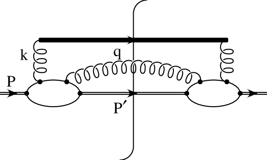
FIG. 9.: Diagram contributing to the diffractive gluon distribution in a meson in the model of this appendix.

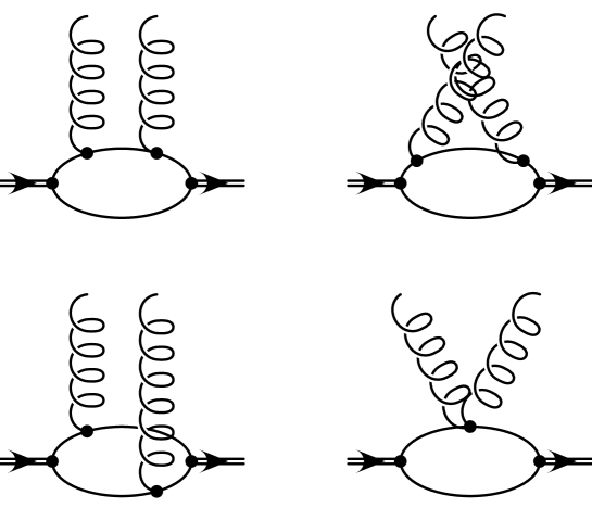
FIG. 10.: Four graphs for the amplitude in Fig. (9)

The final form for $G_{g/A}^{{\rm diff}}$ that we obtain is,

$$G_{g/A}^{{\rm diff}}(P,q,k) = {1\over{2(2\pi)^{3}\beta(1-\beta)x_{{IP}}^{2}}}\int d^{2}{\bf q}\ {{G^{\mu\alpha}(P,q,k)^{*}\ G^{\nu\beta}(P,q,k)\ g_{\alpha\beta}\,c_{\mu\nu}(k)}\over{(k^{2}+i\epsilon)(k^{2}-i\epsilon)}}$$ (B4)

where $k^{+}=\beta x_{{IP}}P^{+}$,

$$c_{\mu\nu}(k) = \frac{1}{(P^{+})^{2}}\ (k^{+2}g_{\mu\nu}+k^{2}g_{\mu}^{+}g_{\nu}^{+}-k_{\mu}k^{+}g_{\nu}^{+}-k_{\nu}k^{+}g_{\mu}^{+}),$$ (B5)

and $G^{\mu\nu}(P,q,k)$ is a second rank tensor containing the sum of quark loops with all possible combinations of attachments by two gluons.

We have evaluated the loop integrals in Eq. (B4) in terms of their explicit Spence function expressions. For this we have used the computer code of G. J. van Oldenborgh and J. A. M. Vermaseren [23]. Their method is an independently formulated extension of the Form algorithm of G. ’t Hooft and M. Veltman [24]. The authors of [23] claim that their algorithms provide easier isolation of both asymptotic behavior and potential numerical instabilities. In one of the most sensitive regions, that of low $t$, their algorithms have proven to be more accurate.

To summarize the specifications of our calculation, it was for small $t$, one external line was massless, and one had to integrate over a large region in the transverse space of the variable ${\bf q}$. Due to gauge invariance, several constraints are placed on $G^{\mu\nu}$ which we have numerically checked to hold. $G^{\mu\nu}(P,q,k)$ has the form

$$G^{\mu\nu}(P,q,k)=\sum_{J=1}^{5}T_{J}^{\mu\nu}A_{J}\,.$$ (B6)

Here the $T_{J}$ are tensors made from the available vectors $P,q,k$. The $A_{J}$ are scalar functions of the dot products of these momenta. In general there would be ten terms in the sum, but gauge invariance cuts this in half. To find the possible $T_{J}$, define

$$P_{q}^{\mu} = q^{2}\,P^{\mu}-P\cdot q\,q^{\mu}\,,$$ (B7)

$$P_{k}^{\nu} = k^{2}\,P^{\nu}-P\cdot k\,k^{\nu}\,,$$ (B8)

$$S_{q}^{\mu} = k\cdot q\,P^{\mu}-P\cdot q\,k^{\mu}\,,$$ (B9)

$$S_{k}^{\nu} = q\cdot k\,P^{\nu}-P\cdot k\,q^{\nu}\,.$$ (B10)

Notice that $q\cdot P_{q}=0$, etc. Now define

$$T_{1}^{\mu\nu} = P_{q}^{\mu}P_{k}^{\nu}\,,$$ (B11)

$$T_{2}^{\mu\nu} = P_{q}^{\mu}S_{k}^{\nu}\,,$$ (B12)

$$T_{3}^{\mu\nu} = S_{q}^{\mu}P_{k}^{\nu}\,,$$ (B13)

$$T_{4}^{\mu\nu} = S_{q}^{\mu}S_{k}^{\nu}\,,$$ (B14)

$$T_{5}^{\mu\nu} = q\cdot k\,g^{\mu\nu}-k^{\mu}q^{\nu}\,.$$ (B15)

These have the property that they are polynomials in the components of the momenta and that $q_{\mu}T_{J}^{\mu\nu}=0$ and $k_{\nu}T_{J}^{\mu\nu}=0$. Thus $G^{\mu\nu}$ is properly gauge invariant. In our calculation, we transformed $G^{\mu\nu}$ into a basis where the first five tensor forms are those given above and the other five are

$$T_{6}^{\mu\nu} = P_{k}^{\mu}P_{q}^{\nu}\,,$$ (B16)

$$T_{7}^{\mu\nu} = P_{k}^{\mu}S_{q}^{\nu}\,,$$ (B17)

$$T_{8}^{\mu\nu} = S_{k}^{\mu}P_{q}^{\nu}\,,$$ (B18)

$$T_{9}^{\mu\nu} = S_{k}^{\mu}S_{q}^{\nu}\,,$$ (B19)

$$T_{10}^{\mu\nu} = g^{\mu\nu}.$$ (B20)

We have checked over a wide range of the parameters $x_{IP}$, $t$ and the transverse momentum ${\bf q}$ that the coefficients of the tensors in Eq. (B20) vanish, leaving only the tensors in Eq. (B15) with nonvanishing coefficients. As a second check for gauge invariance of $G^{\mu\nu}$, we have numerically checked that $q_{\mu}G^{\mu\nu}=0$ and $k_{\nu}G^{\mu\nu}=0$.

In Fig. 11 we show the diffractive gluon distribution function multiplied by $\beta x_{IP}$, at $|t|=1{\ \rm GeV}^{2}$, and for a selected choice of $x_{IP}$ values. The masses of the quarks and mesons were $M^{2}=m^{2}=0.1{\ \rm GeV}^{2}$, while the couplings were $G=0.3{\ \rm GeV}$ and $g=0.1$. We see that the model does not exhibit the behavior

$${{df^{\rm diff}_{g/A}(\beta x_{IP};x_{IP},t)}\over{dx_{IP}\,dt}}\propto x_{IP}^{-2}$$ (B21)

for $x_{IP}\to 1$ at fixed $\beta$ that would be characteristic of pomeron exchange. One needs at least one rung of a gluon ladder to obtain this behavior. The model exhibits the behavior

$${{df^{\rm diff}_{g/A}(\beta x_{IP};x_{IP},t)}\over{dx_{IP}\,dt}}\propto(1-\beta)^{0}$$ (B22)

as $\beta\to 1$ at fixed $x_{IP}$, as in Eq. (74).

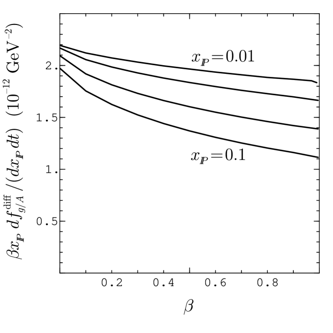
FIG. 11.: Diffractive gluon distribution $\beta x_{IP}\,df_{g/A}^{\rm diff}(\beta x_{IP};x_{IP},t)/dx_{IP}\,dt$ in the model of this appendix as a function of $\beta$ for (from top to bottom) $x_{IP}$=0.01, 0.02, 0.05, 0.1 with $|t|=1\ {\rm GeV}$ In this model, there is no dependence on a renormalization scale $\mu$. The parameter choices are $M^{2}=m^{2}=0.1{\ \rm GeV}^{2}$, $G=0.3{\ \rm GeV}$ and $g=0.1$

One can understand the $\beta$ and $x_{{IP}}$ behavior seen in this numerical study from an analytic viewpoint. In Sec. VII, the detected and emitted gluons coupled do a slow gluon. In the present simple model, they couple directly to a fast quark. This means that the virtual quark line in Fig. 9 is far off shell when ${\bf q}^{2}/((1-\beta)x_{IP})\gg m^{2}$. For example, it is off shell for ${\bf q}^{2}\sim m^{2}$ for any $\beta$ as long as we take $x_{IP}\ll 1$. This gives quite a different behavior from that found in Sec. VII. In the model, the loop serves as a built-in low momentum cut-off. However, the meson can be replaced by a single fast quark line if we substitute an artificial low momentum cut-off

$${\bf q}^{2}>(1-\beta)x_{IP}\ m^{2}$$ (B23)

Then a simple power counting analysis gives,

$${df^{\rm diff}_{g/A}(\beta x_{IP};x_{IP},t)\over dx_{IP}\,dt}\sim{{\rm const.}\over(1-\beta)x_{IP}^{2}}\ \int_{0}^{\infty}dq_{T}^{2}\ {\theta(q_{T}^{2}>(1-\beta)\,x_{IP}\,m^{2})\over\{q_{T}^{2}/[(1-\beta)\,x_{IP}]\}^{2}}$$ (B24)

for $x_{IP}\ll 1$ and $(1-\beta)\ll 1$. Performing the integral gives

$$\frac{df^{\rm diff}_{g/A}(\beta x_{IP};x_{IP},t)}{dx_{IP}\,dt}\sim(1-\beta)^{0}x_{{IP}}^{-1}.$$ (B25)

This agrees with our numerical findings. We find it reassuring that a fully consistent field theoretic calculation of the diffractive gluon distribution gives results that agree with expectations similar to our analytic arguments in Sec. VII.

REFERENCES

- [1] ZEUS Collaboration (M. Derrick, et al.), Phys. Lett. B315, 481 (1993); B332, 228 (1994); B338, 483 (1994); preprint DESY 95-093 (Archive: hep-ex@xxx.lanl.gov - 9505010); H1 Collaboration, (T. Ahmed et al.), Nucl. Phys. B429, 477 (1994); Phys. Lett. B348, 681 (1995).
- [2] G. Ingelman and P. Schlein, Phys. Lett. 152B, 256 (1985).
- [3] E. L. Berger, J. C. Collins, D. E. Soper, and G. Sterman, Nucl. Phys. B286, 704 (1987).
- [4] A. Brandt, et. al., Phys. Lett. B297, 417 (1992).
- [5] A. Berera and D. E. Soper, Phys. Rev. D 50, 4328 (1994).
- [6] G. Veneziano and L. Trentadue, Phys. Lett. B323, 201 (1993).
- [7] A. Donnachie and P. V. Landshoff, Phys. Lett. B B191, 309 (1987); Nucl. Phys. B303, 634 (1988).
- [8] See, for example, E. Gotsman, E. M. Levin, U. Maor, Z. Phys. C 57, 677 (1993); J. Bartels and E. Levin, Nucl. Phys. B387, 617 (1992); J. Bartels, Nucl. Phys. A546, 107c (1992).
- [9] J. C. Collins and D. E. Soper, Nucl. Phys. B194, 445 (1982).
- [10] G. Curci, W. Furmanski and R. Petronzio, Nucl. Phys. B175, 27 (1980).
- [11] V. N. Gribov and L. N. Lipatov, Sov. J. Nucl. Phys. 15, 438 (1972); L. N. Lipatov, Sov. J. Nucl. Phys. 20, 93 (1975); Yu. L. Dokshitzer, Sov. Phys. JEPT 56, 641 (1977); G. Altarelli and G. Parisi, Nucl. Phys. B26, 298 (1978).
- [12] J. C. Collins, D. E. Soper, and G. Sterman, Nucl. Phys. B261, 104 (1985); B308, 833 (1988).
- [13] G. Bodwin, Phys. Rev. D 31, 2616 (1985); 34, 3932 (1986).
- [14] J. C. Collins, L. Frankfurt, and M. Strikman, Phys. Lett. B307, 161 (1993).
- [15] A. Donnachie and P. V. Landshoff, Nucl. Phys. B231, 189 (1984); B244, 322 (1984).
- [16] J. C. Collins, in Physics Simulations at High Energy edited by V. Barger, T. Gottschalk, and F. Halzen (World Scientific, Singapore, 1987).
- [17] V. S. Fadin, E. A. Kuraev, and L. N. Lipatov, Phys. Lett. B60, 50 (1975); I. Balitsky and L. N. Lipatov, Sov. J. Nucl. Phys. 15 438 (1978).
- [18] H1 Collaboration (T. Ahmed et al.), Nucl. Phys. B439, 471 (1995); ZEUS Collaboration (M. Derrick, et al.), Z. Phys. C65, 379 (1995).
- [19] A. Capella, A. Kaidalov, C. Merino, D. Pertermann and J. Tran Thanh Van, preprint LPTHE-ORSAY-95-33, May 1995, archive: hep-ph@xxx.lanl.gov - 9506454; K. Golec-Biernat and J. Kwiecinski, Phys. Lett. B353, 329,(1995).
- [20] S. J. Brodsky and G. Farrar, Phys. Rev. Lett. 31, 1153 (1973); Phys. Rev. D 11, 1309 (1975); V. A. Matveev, R. M. Murddyan and A. V. Tavkheldize, Lett. Nuovo Cimento 7, 719 (1973); F. Close and D. Sivers, Phys. Rev. Lett. 39, 1116 (1977); D. Sivers, Ann. Rev. Nucl. Part. Sci. 32 149 (1982).
- [21] F. E. Low, Phys. Rev. D 12, 163 (1975); S. Nussinov, Phys. Rev. Lett. 34, 1286 (1975); Phys. Rev. D 14, 246 (1976); J. F. Gunion and D. E. Soper, Phys. Rev. D 15, 2617 (1977)
- [22] J. C. Collins, J. Huston, J. Pumplin, H. Weerts and J. J. Whitmore, Phys. Rev. D 51, 3182 (1995).
- [23] G. J. van Oldenborgh and J. A. M. Vermaseren, Z. Phys. C 46, 425 (1990).
- [24] G. ’t Hooft and M. Veltman, Nucl. Phys. B153, 365 (1979).