Spherically symmetric quark-gluon plasma field configurations

Abstract

We study field configurations in a hot quark-gluon plasma with spherical symmetry. We show that the electric fields point into radial direction and solve the effective non-abelian equations of motions. The corresponding charge density has a localized contribution which has a gauge invariant interpretation as a pointlike color charge. We discuss configurations oscillating periodically in time. Furthermore, we calculate the electric field induced by a constant local charge that is removed from the plasma for $t>0$ as a model of a decaying heavy quark.

Introduction

Unlike as QED where linear-response theory supplies a straight-forward definition of the Debye-screening potential as the energy induced by a static delta-like charge distribution, the non-abelian analog is not a gauge invariant way to couple a classical charge to the gauge potentials. Making the perturbed Hamiltonian gauge invariant generally amounts to include ghost fields which compensate for the trivial transformation behavior of the classical field strength. It was argued [1] that particularly in the temporal gauge ($A_{0}=0$) the gauge potentials and fields are related in a quasi-abelian way by $\vec{E}=-\partial^{0}\vec{A},$ rendering the abelian response-theory applicable.

The TAG, however, does not admit an imaginary time formalism (ITF) in the usual way [2], and a reformulation in the so-called physical phase space formulation [3] again would call for the inclusion of vertices in the linear response function necessary to account for the non-abelian character of the theory.

In order to avoid these difficulties one may consider the electric dispersion relation without external sources and define the screening potential as the Fourier-transform of the static propagator on the physical dispersion. I want to point out that taking the static limit $\Pi(k_{0}=0,\vec{k})$ alone does not define a gauge invariant potential, and thus a physical quantity. Although the leading order static self energy is just a constant, $\Pi_{el}(k_{0},\vec{k})=m^{2}=g^{2}T^{2}(N+N_{f}/2)/3$, a next-to leading order definition requires the inclusion of the physical dispersion. In the case that the propagator had a pole well separated from eventually cut contributions, the pole really corresponds to a physical observable [4]. However, due to mass-shell singularities appearing within the standard resummation scheme [5], the longitudinal self energy turns out to be sensible to a – perturbatively uncalculable – magnetic mass [6]. Although the electric self-energy does develop a gauge invariant pole at next-to-leading order, it is not clear to what observable this quantity corresponds.

In this paper we study spherically symmetric field configurations at leading order which have an interpretation as generated by a local charge in a gauge invariant way.

I Observables for spherical symmetry

Let us reconsider the generic idea to put a pointlike static quark in the hot quark-gluon plasma. A classical source may be characterized by the following properties.

• The source is assumed to have no internal structure such as spin which would involve a magnetic moment.

• The source is localized and pointlike, and its location is static with respect to the rest frame of the plasma. Since at finite temperature essentially infrared physics is concerned, one can in fact exclude the location of the charge as singular region from space-time. To make this statement more precise, we consider physics only at distances greater or equal $T$ away from the hypothetical classical source.

From (i) and (ii) it follows that observables have to be spherically symmetric. Let us illustrate that those two assumptions are sufficient in classical electrodynamics to single out the Coulomb potential as the only solution, up to a multiplicative factor. The fields satisfy the sourceless Maxwell equations,

$$\vec{\partial}\vec{E}=0,\quad\vec{\partial}\times\vec{B}-\dot{\vec{E}}=0,\quad\vec{\partial}\times\vec{E}+\dot{\vec{B}}=0,\quad\vec{\partial}\vec{B}=0$$ (1)

and are spherically symmetric. Due to the famous theorem saying that ’you cannot comb a hedgehog’, spherically symmetric vector fields can always be written as a gradient of a scalar in three dimensions, to wit

$$\vec{E}(r,t)=\frac{\vec{r}}{r}E(r,t)\quad \Rightarrow \quad\vec{E}(r,t)=\vec{\partial}f(r,t)$$ (2)

$$\vec{B}(r,t)=\frac{\vec{r}}{r}B(r,t)\quad \Rightarrow \quad\vec{B}(r,t)=\vec{\partial}g(r,t).$$ (3)

It follows from the Gauss law that

$$\Delta f(r,t)=0\quad\Rightarrow\quad f(r,t)=a(t)+\frac{b(t)}{r}\quad\Rightarrow\quad\vec{E}(r,t)=b(t)\;\vec{\partial}\frac{1}{r}\quad$$ (4)

and from the second Maxwell-equation in (1) $\dot{\vec{E}}=\vec{\partial}\times\vec{B}=\vec{\partial}\times\vec{\partial}g=0,$ thus $\dot{b}(t)=0$ and the electric field $\vec{E}\propto\vec{r}/r^{3}$ corresponds to the Coulomb potential.

Turning to the non-abelian case, the symmetry properties (3) cannot be imposed directly on the fields, since those are not gauge invariant quantities. According to their transformation behavior we are able to distinguish two classes of quantities in a gauge theory, these which transform inhomogeneously as the gauge potentials,

$$A_{\mu}\to U^{-1}A_{\mu}U+\frac{1}{ig}U^{-1}\partial_{\mu}U$$ (5)

and those that transform homogeneously

$$\vec{E}\to U^{-1}\vec{E}U$$ (6)

as the electric and magnetic fields, the charge and the spatial current. That quantities will be called pre-gauge invariant since the trace of products of them defines observables. Operators that have positive and gauge invariant eigenvalues correspond to physical quantities, and the eigenvalue is the physical observable. Considering e.g. the eigenvalue problem of the Lie-group valued electric fields

$$\hat{\vec{E}}(\vec{x},t)\left|E(\vec{x})\right\rangle=\vec{E}(\vec{x},t)\left|E(\vec{x})\right\rangle$$ (7)

where the hermitian field operator $\hat{\vec{E}}(\vec{x},t)$ is taken in the Heisenberg-representation, it is obvious that the eigenvalue is real and remains unchanged under unitary (gauge) transformations (6). In that sense all pre-gauge invariant quantities potentially correspond to physical observables. In order to construct a set of equal time observables, however, we need those operators to commute with each other. As concerns the Lie algebra $\mathrm{su(N)}$ one may chose a Cartan-Weyl representation with the basis elements $T^{s},\,s=1,\ldots,r,\,r=\mbox{rank of the algebra}$, spanning the abelian Cartan subalgebra and the remaining $n-r$ generators $T^{\pm a}$ where $a$ is an r-dimensional root vector. A set of commuting variables is given by the diagonal components $\vec{E}^{s}T^{s}$ (no sum over s) and the hermitian commutators

$$\left[E^{i,a}T^{a},(E^{i,a}T^{a})^{\dagger}\right]=E^{i,a}(E^{i,a})^{*}\;\sum_{s}a(s)T^{s}\quad\mbox{(no sum over $i$ and $a$) }$$ (8)

where $a(s)$ is some weight depending on the group under consideration. Imposing spherical symmetry restricts the real diagonal components $\vec{E}^{s}$ analogously to the abelian case (3), whereas only the modulus of the complex components $\vec{E}^{a}$ of the roots is subject to the symmetry,

$$\vec{E}^{a}=\frac{\vec{r}}{r}|E^{a}(r,t)|{\mathrm{e}}^{i\chi^{a}(r,\Omega,t)}.$$ (9)

This can also be seen directly by considering the eigenvalues of the eigenvalue problem (7) where only products like $E^{a}E^{-a}=E^{a}(E^{a})^{*}$ enter. Moreover, on account of the commutator $[T^{s},T^{a}]=a(s)T^{a}$, the phase of one additional non-diagonal color component in (9) can be absorbed with the help of the local gauge transformation $U=\exp(iT^{s}\chi^{a}/a(s))$ which leaves the abelian part $E^{s}T^{s}$ invariant. This shows, that in a spherically symmetric situation, only $r+1$ ($N$ for SU(N) ) components of pre-gauge invariant variables can been chosen to depend on the radial coordinate and time, but the vector component of the variables has always to point in radial direction as in the abelian case.

One could also consider the more general situation where external space-time and internal symmetries mix. For $\mathrm{SU}(2)$ as internal symmetry group, this leads to an enlarged number of solutions of the Maxwell equations [7], but is in principle restricted to the case where internal and external symmetry groups are locally isomorphic i.e.  $\mathrm{O(3)}\sim\mathrm{SU(2)}$.

II Spherically symmetric field configurations in a hot quark-gluon plasma

Let us now turn to the similar situation in a hot quark-gluon plasma. For field strengths of order of the temperature, $A\sim T$, and in the long wavelength limit, $\partial\sim gT$, the Maxwell-equations without external source generalize to [8]

$$\left[D_{\mu},F^{\mu\nu}\right]=j_{\mathrm{ind}}^{\nu}$$ (10)

where $D^{\mu}=\partial^{\mu}+ig\left[A^{\mu},\;.\;\right]$ and $F^{\mu\nu}=\left[D^{\mu},D^{\nu}\right]/(ig)$. In that regime the full non-abelian character of the theory enters, and one cannot expand the covariant derivative in a series in the coupling constant. The induced current $j_{\mathrm{ind}}^{\mu}$ describes the response of the plasma to the non-abelian gauge fields and has to be a covariantly conserved quantity

$$\left[D_{\mu},j^{\mu}\right]=0$$ (11)

for consistency with the Maxwell equations (10). It can be expressed by means of an auxiliary field $W^{\mu}$

$$j^{\mu}_{\mathrm{ind}}(x)=m^{2}\int\frac{\mathrm{d}\Omega_{v}}{4\pi}v^{\mu}W^{0}(x,v)$$ (12)

where $v^{\mu}=(1,\vec{v})$ denotes a null vector and the angular integral $\int\mathrm{d}\Omega$ runs over all directions of $\vec{v}$. $W^{\mu}$ is a solution to

$$\left[v\cdot D,W^{\mu}\right]=F^{\mu\nu}v_{\nu}$$ (13)

and conjugate to $v^{\mu},$ $v_{\mu}W^{\mu}=0.$ The set of equations (10,12) and (13) forms a complicated highly non-linear system of integro-differential equations describing the long wavelength behavior of a hot quark-gluon plasma. A particular class of plain-wave solutions where the gauge potential depends on space-time only as a function of $(p\cdot x)$ has been found in [9].

Here, we will consider spherically symmetric configurations with vanishing magnetic fields $B^{i}=\epsilon^{ijk}F_{jk}=0$. Note that under a gauge transformation $\vec{B}$ transforms homogeneously as the electric field (6) so that solutions with vanishing magnetic fields have a gauge invariant meaning. Moreover, those configurations are singled out in the sense that the spatial components of the corresponding gauge potentials can always be written as pure gauge,

$$\vec{A}=\frac{1}{ig}V^{-1}\vec{\partial}V,$$ (14)

with $V$ being a space-time dependent element of the gauge group. In that case the gauge potentials even become pre-gauge invariant quantities. This class of solutions could also have been obtained by assuming the gauge fields to be spherically symmetric in the first place, which also leads to vanishing magnetic fields. However, as pointed out above, gauge potentials a priori have no meaning as observables and thus assuming them to be radially symmetric is rather an ansatz than a necessary consequence imposed by a symmetry condition.

With the particular form of the potential (14) it is now possible to find radially symmetric solutions of the Maxwell equations. For this purpose we note that the covariant derivative of a group valued quantity $X$ can be rewritten in the form

$$\left[\vec{D},X\right]=V^{-1}\left(\vec{\partial}(VXV^{-1})\right)V,$$ (15)

which suggests the introduction of the gauge equivalent quantities

$$\vec{\mathcal{E}}=V{\vec{E}}V^{-1},\quad{\mathcal{Q}}=V\rho_{\mathrm{ind}}V^{-1},\quad{\mathcal{W}}^{0}=VW^{0}V^{-1}.$$ (16)

Thus the Gauss-law and the zeroth component of (13)

$$[\vec{D},\vec{E}]=\rho_{\mathrm{ind}},\quad\left[v\cdot D,W^{0}\right]=F^{0i}v_{i}=-\vec{E}\vec{v}$$ (17)

assume quasi-abelian form

$$\vec{\partial}\vec{\mathcal{E}}={\mathcal{Q}},\quad(v\cdot\partial)\;{\mathcal{W}}^{0}=-\vec{\mathcal{E}}{\vec{v}}.$$ (18)

We may further choose the spatial components of $v$ to point into radial direction, $\vec{v}=\vec{r}/r.$ This entails that the spatial components of the induced current in (12) vanishes and the induced charge becomes proportional to ${\mathcal{W}}^{0}$,

$${\mathcal{Q}}(r,t)=m^{2}\int\frac{\mathrm{d}\Omega}{4\pi}{\mathcal{W}}^{0}(r,t)=m^{2}{\mathcal{W}}^{0}(r,t).$$ (19)

Due to the linearity of Eq. (18) and the particular form (9), the diagonal color components of the electric field satisfy the differential equation

$$(\partial_{0}+\partial_{r})(\frac{2}{r}+\partial_{r}){\mathcal{E}}=m^{2}{\mathcal{E}}$$ (20)

which will be in the center of our further investigations.

We construct solutions in terms of eigenfunctions of the time derivative, ${\mathcal{E}}(r,t)={\mathcal{E}}(r){\mathrm{e}}^{i\omega t}$ where the separation parameter $\omega$ may in general assume complex values. Eq. (20) can be straightforwardly transformed into the radial Schrödinger-equation for the hydrogen atom

$$\frac{d^{2}}{d\rho^{2}}\left({\mathrm{e}}^{i\omega r/2}{\mathcal{E}}(\rho)\right)+\frac{2}{\rho}\frac{d}{d\rho}\left({\mathrm{e}}^{i\omega r/2}{\mathcal{E}}(\rho)\right)+\left(-\frac{2}{\rho^{2}}+\frac{i\omega}{\kappa\rho}-\frac{1}{4}\right)\left({\mathrm{e}}^{i\omega r/2}{\mathcal{E}}(\rho)\right)=0$$ (21)

with $\kappa=\sqrt{4m^{2}-\omega^{2}}$ and $\rho=\kappa r$. The solution of (20) is composed of a singular and a regular part,

$${\mathcal{E}}(r)=\frac{{\mathrm{e}}^{-(\kappa+i\omega)\frac{r}{2}}}{4\pi r^{2}}\left(\frac{C_{1}}{2}\Gamma(2-i\frac{\omega}{\kappa})U(-1-i\frac{\omega}{\kappa},-2,\kappa r)+C_{2}r^{3}M(2-i\frac{\omega}{\kappa},4,\kappa r)\right)$$ (22)

where $U$ and $M$ denote the confluent hypergeometric functions [10], $C_{1},C_{2}$ are constants and the additional factor in front of the first term is chosen such that the series in $r$ of the first summand in the brackets starts with unity.

The quantity $i\omega/(\kappa\rho)$ which is the charge of the nucleus in the corresponding quantum mechanical problem, is an imaginary number for real $\omega$. This entails that $\kappa$ becomes purely imaginary when the first argument in the hypergeometric function $M$ is a negative integer and its power series terminates. Consequently, no stationary regular bounded solutions – corresponding to the quantum mechanical bound states – exist.

The singular part proportional to $U$ which is usually excluded by the demand of regularity at the origin has in fact an interpretation as the electric field generated by a pointlike source. Let us ’measure’ the charge corresponding to that field according to (18). More precisely, we consider the divergence of ${\mathcal{E}}$ in the sense of distributions acting as a functional on $C_{0}^{\infty}({{\mathbb{R}}}^{3})$ test functions $\varphi$,

$$\left({\mathcal{Q}},\varphi\right)=-\left(\vec{\mathcal{E}},\vec{\partial}\varphi\right):=-\int d\Omega\int_{0}^{\infty}drr^{2}\vec{\mathcal{E}}(r)\vec{\partial}\varphi(r\Omega)$$ (23)

which by integration by parts leads to

$$\lim_{r\to 0}(4\pi r^{2}{\mathcal{E}}(r))\varphi(0)+\int d\Omega\int_{0}^{\infty}drr^{2}\left(\frac{(r^{2}{\mathcal{E}}(r))^{\prime}}{r^{2}}\right)\varphi(r\Omega)=:C_{1}(\delta^{3},\varphi)+(\vec{\partial}\vec{\mathcal{E}},\varphi).$$ (24)

The resulting charge is composed of a pointlike source $\propto\delta^{3}(r)$ which gets contributions only from the singular part of the electric field and the divergence which corresponds to the charge induced by the plasma. In what follows we will not consider the true vacuum solution $\propto M$ and concentrate on to physically more interesting situations with local charges. Particularly, we focus on an oscillating point charge and a charge which is constant for $t<0$ and vanishes for $t\geq 0$.

A Monochromatic oscillations

One particularly interesting class are stationary plasma waves induced by a periodically oscillating charge, ${\mathcal{Q}}^{\mathrm{local}}(r,t;\omega)=\delta^{3}(r){\mathrm{e}}^{i\omega t}$ which electrical field is given by (22) multiplied by ${\mathrm{e}}^{i\omega t}$ with $C_{1}=1$ and $C_{2}=0$. Above the frequency $\bar{\omega}=2m$, the inverse damping length $\kappa$ becomes an imaginary quantity, and we choose the root such that $\Im(\kappa)<0$. The exponentially decreasing radial dependence in (22) turns into a radially periodic one. The hypergeometric function $U$ increases for large radial distances like $r^{1+i\omega/\kappa}$ which combines with the prefactor to $r^{-1+i\omega/\kappa}<r^{-1}$.

For very large frequencies, $\kappa\to-i\omega$, the hypergeometric function independently from $r$ becomes unity, and the radial dependence of the exponential vanishes. In this case, the electric fields $\propto\exp(i\omega t)/r^{2}$ cease to propagate in the plasma.

In the other extreme of a static charge, i.e. for $\omega\to 0$, the electric field $\propto{\mathrm{e}}^{-mr}(1+mr)/r^{2}$ corresponds to the exponentially screened Debye potential.

It is instructive to consider the situation of perturbations with periods corresponding to mass threshold $\bar{\omega}$. In that case the damping length $1/\kappa$ becomes infinite and the argument in the gamma function in (22) diverges. However, the infinities are just compensated by the hypergeometric function and one finds in the limit $\kappa\to 0$

$${\mathcal{E}}^{\omega=2m}(r,t)=m^{2}\frac{(2ix)^{3/2}}{x^{2}}{\mathrm{e}}^{2iy-ix}K_{3}(2\sqrt{2ix})$$ (25)

where $x=mr$, $y=mt$, and $K_{3}$ denotes the Neumann function of imaginary argument. The large distance behavior is somehow in between the static exponential decrease and the high frequency power-law behavior. In fact, asymptotically expanding the Bessel function,

$${\mathcal{E}}^{\omega=2m}(r,t) = \frac{\sqrt{\pi}m^{2}}{2x^{2}}{(2ix)^{5/4}}\thinspace{\mathrm{e}}^{2iy-ix-2\sqrt{2ix}}\left(1+\frac{35}{16\sqrt{2ix}}+{\mathcal{O}}\left(\frac{1}{x}\right)\right)$$ (26)

$$= \frac{\sqrt{\pi}m^{2}}{2x^{2}}{(2ix)^{5/4}}\thinspace\exp\left(2iy-ix-2(1+i)\sqrt{x}-\frac{i\pi}{8}+\frac{35(1-i)}{32\sqrt{x}}+{\mathcal{O}}\left(\frac{1}{x}\right)\right)$$ (27)

shows that the field is damped with an exponential $\propto\sqrt{x}$ only. The phase gets also contributions from $\sqrt{x}$, a constant term and inverse powers of the root. Asymptotically, constant phases propagate with velocity

$$v_{\phi}=\frac{dx}{dy}=2\left(1-x^{-1/2}+x^{-1}+\frac{29}{64}x^{-3/2}+{\mathcal{O}}(x^{-2})\right)$$

which approaches twice the speed of light for $x\to\infty$. Physical information about the propagation of waves in the plasma may be deduced from the acceleration of the phase velocity,

$$\frac{dv_{\phi}}{dy}=v_{\phi}\frac{dv_{\phi}}{dx}\sim 2x^{-3/2}-6x^{-2}+\frac{279}{32}x^{-5/2}+{\mathcal{O}}(x^{-2}).$$

The leading coefficient has a positive sign which means that a maximum of the oscillation runs slightly faster away from the origin than its neighboring maximum remoter from the source. A similar study in the regime $x\lesssim 1$ shows that also there waves appear accelerated in positive radial direction with a maximal acceleration at $x\sim 0.3$ (Fig1.).

FIG. 1.: Phase speed (left) and phase acceleration (right) of the electric field in function of the distance of a localized charge periodically oscillating with frequency $2m$.

B Shock wave of a suddenly removed point charge

In this section we study the situation where the localized charge is constant for $t<0$ and vanishes for $t\geq 0$. In a physical experiment, the charge may be a heavy quark which due to its large mass can be thought of as a well localized classical color source. At $t=0$ the quark may decay into a number of lighter particles which can escape the plasma or be thermalized depending on their energy, the temperature and the size of the plasma. In any case, we are faced with a scenario of a – with respect to the typical time scale $m$ of the plasma – suddenly disappearing color-charge.

To model the situation we have to find a superposition of the monochromatic oscillating solutions studied in the last section. This can be easily achieved by observing that the charge can be written as

$$\delta^{3}(r)\theta(-t)=\delta^{3}(r)\frac{i}{2\pi}\int_{\mathcal{C}}d\omega\frac{{\mathrm{e}}^{i\omega t}}{\omega}=\frac{i}{2\pi}\int_{\mathcal{C}}\frac{d\omega}{\omega}Q^{\mathrm{l}ocal}(r,t;\omega).$$ (28)

The path of integration is parallel to the real $\omega$ axes as shown in Fig. 2, and picks up the residue when closed in the lower half plane. The corresponding superposition of the monochromatic electric fields becomes

$${\mathcal{E}}^{\mathrm{s}w}(r,t)=\frac{i}{16\pi^{2}r^{2}}\int_{\mathcal{C}}d\omega\frac{{\mathrm{e}}^{i\omega t-(\kappa+i\omega)\frac{r}{2}}}{\omega}\Gamma(2-\frac{i\omega}{\kappa})U(-1-\frac{i\omega}{\kappa},-2,\kappa r).$$ (29)

Prior to evaluating this integral by closing the contours above and below respectively, we have to define the root $\kappa=\sqrt{4m^{2}-\omega^{2}}$ for complex values of $\omega$. It admits to branch points and it turns out to be most useful to chose the cuts parallel to the imaginary $\omega$-axes. The sign is chosen that $\kappa\to i\omega$ for large modulus of $\omega$ and $|\Re(\omega)|>2m$.

FIG. 2.: Cut and pole structure in the $\omega$-plane of the decaying-particle solution.

This choice admits to close the contour in the lower half plane for $t-r<0$ where the integrand vanishes exponentially on the arc. The only contribution comes from the residuum which gives the static limit

$${\mathcal{E}}^{t<r}(r,t)=\frac{{\mathrm{e}}^{-mr}}{4\pi r^{2}}(1+mr)$$ (30)

corresponding to the Debye potential.

For $t>r$ we may deform the contour to the arc $|\omega|\to\infty,\,\Im(\omega)>0$ on which the integrand vanishes but which picks up two cut-contributions. The contours around the cuts are well separated from the pole which facilitates considerably an asymptotical and numerical evaluation of the integration. In order to calculate the discontinuity we need the relation

$$\Gamma(2-a)U(-1-a,-2,z) - \Gamma(2+a)U(-1+a,-2,-z){\mathrm{e}}^{z}$$ (31)

$$= \frac{a(a^{2}-1)\pi}{6\sin\pi a}z^{3}M(2-a,4,z)$$ (32)

which can readily be derived from the integral representation of the hypergeometric function.

Coosing the parametrization $\omega=2m(-1+iu)$ for the left contribution, we get

$${\mathcal{E}}^{t>r}(r,t)=-m^{2}\frac{ix}{12\pi}\int_{0}^{\infty} du\frac{\exp(-2iy+ix-2yu+xu+x\sqrt{u}\sqrt{u+2i})}{\sin\pi\frac{i+u}{\sqrt{u}\sqrt{u+2i}}}\times$$ (34)

$$M(2-\frac{i+u}{\sqrt{u}\sqrt{u+2i}},4,-2x\sqrt{u}\sqrt{u+2i})+\mathrm{h.c.}$$

where the complex conjugate part stems from the right cut. This expression is a particular superposition of regular solutions corresponding to vanishing local charge since the causal information of the decay propagates in the future directed light cone $t>x$ of the event at $(x=0,t=0)$.

The evaluation of the integral (34) is quite complicated since the integration variable appears not only in the argument but also in the index of the hypergeometric function. For values of $x\sim 1$ and larger, the situation is quite hopeless since even the asymptotic expansion of $M$ for large arguments is spoiled by the diverging index at small $u$ where the integrand contributes most.

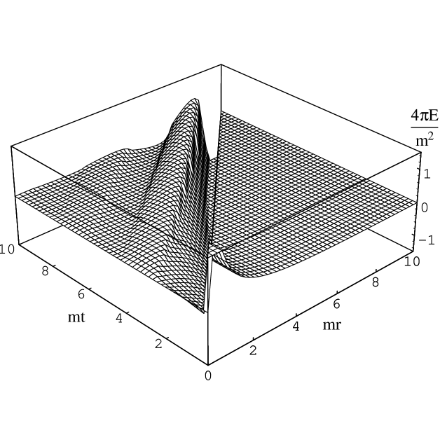
FIG. 3.: The electric shock wave propagating in the plasma. Below the light cone $t<r$ the electric fields correspond to the Debye potential, are hit by the shock wave at $t=r$ and vanish asymptotically for late times in the forward-directed light-cone.

However, a numerical integration is still possible with the result shown in Fig. 3. The graph shows that waves are damped for large distances in direction orthogonal to the light cone. In the region close to the light cone $r\sim t$ the amplitudes increase with the distance of the origin.

III Summary and Conclusion

We studied the spherically symmetric solutions of electric field configurations in a hot quark-gluon plasma. We showed assuming vanishing magnetic fields, which is a necessary compatibility condition with the symmetry imposed, that the electric fields which are a priori no physical observables in a non-abelian theory can nevertheless be given a physical interpretation. As in the abelian case, they are radially directed vector fields. Their physical components can be gauge transformed to depend on time and radius only. Using this property together with the equations of motions in the hard thermal loop approximation, we construct a differential equation for the fields. The solution of that equation consists of a singular and a regular part. Evaluating the corresponding charge in the sense of generalized functions shows that the singularity at the origin corresponds to pointlike charge, and the remaining part has an interpretation a induced charge. This admits to uniquely relate localized charge, induced charge and corresponding electric field in a manifestly gauge invariant way.

We focus on two particular interesting physical situations: A periodically oscillating and a suddenly removed local charge. In the first case, we establish the electric field and concentrate on oscillations with frequencies close to the frequency $2m_{\mathrm{D}ebye}$. The asymptotic field is found to oscillate with amplitude $(mr)^{-3/4}\thinspace{\mathrm{e}}^{-2\sqrt{mr}}$, which is in between the exponentially damped static limit corresponding to the Debye potential and a power-law behavior for oscillations above $\omega=2m$.

In the second example we study a suitably chosen superposition of the periodic solution which has constant local charge for $t<0$ and vanishing local charge for $t>0$. The electric field is found to correspond to the static Debye case for $t<r$. In the causal region $t>r$, the electric field can be written as an integral which we evaluate numerically. The suddenly disappearing charge may be regarded as a model for a heavy, well localized quark placed in a hot quark-gluon plasma which spontaneously decays into a number of lighter particles which can escape the plasma or be thermalized.

We found a gauge invariant concept to replace the QED-inspired idea of putting a local classical source into a plasma that potentially violates gauge invariance in the non-abelian case. We find that symmetry properties, and in particular spherical symmetry, already single out a class of solutions which admit a posteriori an interpretation of a localized charge. That result encourages to look for a symmetry-based definitions of physical observables, and in particular of the Debye mass. Work in that direction is currently under progress.

REFERENCES

- [1] K. Kajantie and J.Kapusta, Ann. Phys. (N.Y.) 169 (1985) 477; U. Heinz, K. Kajantie and T. Toimela, Ann. Phys. (N.Y.) 176 (1987) 218; J. Kapusta, Finite temperature field theory, Cambridge University Press, 1989.
- [2] K. James and P. V. Landshoff, Phys. Lett. B 251 (1990) 167.
- [3] H. Nachbagauer, Finite temperature formalism for non-abelian gauge theories in the physical phase space, preprint ENSLAPP-A-510/95, hep-ph/9503244, To appear in Phys. Rev. D.
- [4] R. Kobes, G. Kunstatter and A. Rebhan, Nucl. Phys. B 355 (1991) 1.
- [5] E. Braaten and R. D. Pisarski, Nucl. Phys. B 337 (1990) 569.
- [6] A. K. Rebhan, Nucl. Phys. B 430 (1994) 319. H. Schulz, Nucl. Phys. B 413 (1994) 353.
- [7] M. Carmeli, Kh. Huleihil and E. Leibowitz, Gauge fields: Classification and equations of motion, World Scientific, Singapore 1989.
- [8] J. P. Blaizot and E. Iancu, Nucl. Phys. B390 (1993) 589, Phys. Rev. Lett. 70 (1993) 3376.
- [9] J. P. Blaizot and E. Iancu, Phys. Lett. B326 (1994) 138; Phys. Rev. Lett. 72 (1994) 3317.
- [10] M. Abramowitz and I. A. Stegun (eds.), Handbook of Mathematical Functions (Dover Publ., New York, 1965).