CERN-TH/95-226

HU-TFT-95-50

IUHET-312

August 27, 1995

GENERIC RULES FOR HIGH TEMPERATURE
DIMENSIONAL REDUCTION AND THEIR
APPLICATION TO THE STANDARD MODEL

K. Kajantie^a, M. Laine^a, K. Rummukainen^b and M. Shaposhnikov^c

^aDepartment of Physics, P.O.Box 9, 00014 University of Helsinki, Finland
^bIndiana University, Department of Physics, Swain Hall West 117,
Bloomington IN 47405 USA
^cTheory Division, CERN,
CH-1211 Geneva 23, Switzerland

Abstract

We formulate the rules for dimensional reduction of a generic finite temperature gauge theory to a simpler three-dimensional effective bosonic theory in terms of a matching of Green’s functions in the full and the effective theory, and present a computation of a generic set of 1- and 2-loop graphs needed for the application of these rules. As a concrete application we determine the explicit mapping of the physical parameters of the standard electroweak theory to a three-dimensional SU(2)$\times$U(1) gauge-Higgs theory. We argue that this three-dimensional theory has a universal character and appears as an effective theory for many extensions of the Standard Model.

1 Introduction

The properties of matter at high temperature are interesting for a number of experimental and cosmological applications. QCD at high temperature and density may be relevant for heavy ion collisions, while finite temperature phase transitions may play an important role in the evolution of the universe. In gauge theories, an entirely analytic perturbative study of the properties of high temperature matter is not possible due to the so called infrared problem in the thermodynamics of Yang-Mills fields [1]. A direct way to compute static equilibrium quantities at high temperature would be to do lattice Monte Carlo simulations in the 4d high temperature theory. However, in many interesting cases the use of the full 4d theory is difficult, if not impossible [2].

These obstacles invoke a demand for a formalism which can solve in a constructive way the problems mentioned. Since a finite temperature equilibrium field theory is equivalent to a zero temperature Euclidean field theory with compact 4th dimension, the idea of the 4d $\rightarrow$ 3d dimensional reduction is natural [3]–[6]. Dimensional reduction means that some properties of the equilibrium high temperature plasma can be derived from a simpler 3d effective theory. The construction of the effective theory is free of IR problems. The 3d theory is purely bosonic, and may then be studied by non-perturbative methods, such as lattice MC simulations. In fact, the idea of dimensional reduction has been around for quite a long time [3, 4]. However, some concrete analytical results for the construction of the 3d effective theory have appeared only recently. They are relevant for the description of the high temperature electroweak phase transition [2],[7]–[13] and high temperature QCD [14]–[19].

The aim of the present paper is the formulation of the general rules of dimensional reduction in a constructive way. Namely, we present a set of 1-loop and 2-loop Feynman diagrams with the results of their computation which can be used for dimensional reduction in any gauge field theory. As an example we construct the 3d effective theory corresponding to the Standard Model of electroweak interactions. New elements here in comparison with [7] are the inclusion of fermions, and the direct relation of the parameters of the effective theory to the physical parameters of the EW theory (the physical Z and W boson, Higgs particle and top quark masses, the muon lifetime and the temperature). We also discuss the strategy for the derivation of the simplest possible effective theory for typical extensions of the electroweak theory, like the models with two Higgs doublets, and the Minimal Supersymmetric Standard Model.

The paper is organized as follows. In Section 2 we formulate the general notion of dimensional reduction and analyse the expansion parameters involved there. In Section 3 we present the building blocks for the construction of the effective theory. Section 4 contains the dimensional reduction of the Standard Model. In Section 5 we relate the parameters in the $\overline{\mbox{\rm MS}}$ scheme to the physical parameters, thus completing the relation of 3d couplings to temperature and observables. Section 6 is a discussion. We argue there that the effective theory of most of the extensions of Standard Model is just the SU(2)$\times$U(1)+Higgs model.

2 Dimensional reduction

The equilibrium properties of matter at high temperatures are related to Matsubara Green’s functions of different field operators. By the concept of dimensional reduction we mean that with some accuracy, all the 4d static bosonic Green’s functions in low energy domain (see below) can be computed with the help of some effective 3d field theory. Let us start with useful definitions.

2.1 Superheavy, heavy and light modes

In order to define dimensional reduction, consider a generic renormalizable field theory at high temperature containing gauge $A_{\mu}$, scalar $\phi$ and fermionic fields $\psi$,

$$L={1\over 4}F_{\mu\nu}F_{\mu\nu}+(D_{\mu}\phi)^{\dagger}(D_{\mu}\phi)+V(\phi)+g_{Y}{\bar{\psi}}\phi\psi+\delta L.$$ (1)

Here the group indices are suppressed, $\delta L$ contains the counterterms, and $V(\phi)$ is of the form

$$V(\phi)=m_{S}^{2}\phi^{\dagger}\phi+\lambda(\phi^{\dagger}\phi)^{2}.$$ (2)

For power counting let us assume that $\lambda\sim g^{2}$ and $g_{Y}\sim g$, where $g$, $\lambda$ and $g_{Y}$ are the gauge, scalar, and Yukawa couplings, respectively. Write all 4d Matsubara fields in the form

$$\phi(x,\tau)=\sum_{n=-\infty}^{\infty}\phi_{n}(x)\exp(i\omega^{b}_{n}\tau),$$ (3)

$$\psi(x,\tau)=\sum_{n=-\infty}^{\infty}\psi_{n}(x)\exp(i\omega^{f}_{n}\tau),$$ (4)

where $\omega^{b}_{n}=2n\pi T,~{}\omega^{f}_{n}=(2n+1)\pi T$ are the 3d tree masses for the bosonic ($\phi_{n}$) and fermionic ($\psi_{n}$) 3d fields. Consider the 1-loop corrections (for definiteness in the $\overline{\mbox{\rm MS}}$-scheme) to the masses of the static modes $\phi_{0}$ from the modes $\phi_{n\neq 0}$ and $\psi_{n}$. In general, they have the form

$$m_{i}^{2}(T)=\gamma_{i}T^{2}+m_{i}^{2},~{}~{}\gamma_{i}\sim g^{2},$$ (5)

where $m_{i}^{2}$ is the zero-temperature mass of the scalar field evaluated at some scale $\mu_{T}^{m}$ (see below, and [7]). In general, $m^{2}(T)$ may be matrices, and in the discussion below we mean the eigenvalues of those. For the spatial components of the gauge fields $\gamma_{i}=0,~{}m_{i}^{2}=0$; for the temporal components of the gauge fields $\gamma_{i}\neq 0,~{}m_{i}^{2}=0$; for the scalar fields $\gamma_{i}\neq 0,~{}m_{i}^{2}\neq 0$. Now, let us divide the masses into different categories depending on their magnitude at high temperature. The 3d masses of all fermionic modes and all bosonic modes with $n\neq 0$ are proportional to $\pi T$, and we will call these modes superheavy. The masses of the temporal components of the gauge fields $A_{0}$ are proportional to $gT$, and these modes are called heavy. The scalar fields can be separated in two different groups. If $m_{i}^{2}$ is different from $-\gamma_{i}T^{2}$, the scalar mass is proportional to $gT$, and the field corresponding to this mass is “heavy”. In the contrary, one may be close to a tree-level phase transition temperature so that $\gamma_{i}T^{2}$ and $m_{i}^{2}$ cancel each other. Then $m_{i}^{2}(T)\sim(g^{2}T)^{2}$, and we call this field “light”. We denote a generic light scalar mass by $m_{3}^{2}$. All spatial components of the gauge fields are “light” because for them $\gamma_{i}=0$.

After these definitions we are ready to explain the conjecture behind dimensional reduction. Two levels of dimensional reduction are usually considered. On the first level the effective theory is constructed for the light and heavy modes (superheavy modes are “integrated out”). The second level is the theory for the light modes only. In this paper we require the 3d Lagrangian of the effective theory to be super-renormalizable, so that scalar self-interactions are at most quartic. The super-renormalizable character introduces an absolute upper bound on the accuracy of the description of the 4d world by a 3d theory, to be discussed below.

2.2 Two levels of dimensional reduction

The theory for light and heavy modes. This theory is valid up to momenta $k\ll T$, but $k$ may be as large as $gT$. Consider a (super)renormalizable 3d gauge-Higgs theory with the Lagrangian

$$L={1\over 4}F_{ij}F_{ij}+(D_{i}\phi)^{\dagger}(D_{i}\phi)+V_{3}(\phi,A_{0})+{\frac{1}{2}}(D_{i}A_{0})^{2}+\delta L,$$ (6)

where $V_{3}(\phi,A_{0})$ is of the form

$$V_{3}(\phi,A_{0})=m^{2}\phi^{\dagger}\phi+\lambda_{3}(\phi^{\dagger}\phi)^{2}+h_{3}\phi^{\dagger}\phi A_{0}^{2}+\frac{1}{2}m_{D}^{2}A_{0}^{2}+\frac{1}{4}\lambda_{A}A_{0}^{4}.$$ (7)

The gauge couplings $g_{3}$ have the dimension GeV^1/2 and the scalar couplings $\lambda_{3}$ the dimension GeV. To leading order, the parameter $m_{D}\sim gT$ is nothing but the Debye mass. Consider bosonic static $n$-point one-particle-irreducible Matsubara Green’s functions $G^{(4)}_{n}(\vec{k}_{i})$ for the light and heavy fields in the full 4d theory, multiplied by factor $T^{n/2-1}$ to have the dimension GeV^3-n/2, and depending on external 3-momenta $\vec{k}_{i}$. The statement of dimensional reduction is that there is a mapping of the temperature and the 4d coupling constants of the underlying theory to the 3d theory such that the 3d theory gives the same light and heavy Green’s functions as the full 4d theory for $k\leq gT$ up to terms of order $O(g^{4})$,

$$\frac{\Delta G}{G}\sim O(g^{4}).$$ (8)

Fourth order in $g$ appears from a powercounting estimate of the contributions of the neglected 6-dimensional operators to typical Green’s functions. For example, the operator $g^{6}\phi^{2}A_{0}^{4}/T^{2}$ contributes to the 2-point scalar correlator at order $g^{6}m_{D}^{2}\sim g^{8}T^{2}$. Since the order of magnitude of $m_{3}^{2}$ is $g^{4}T^{2}$, the relative error is $O(g^{4})$. The same estimate arises by comparing the contribution of the neglected operator $g^{2}(k^{4}/T^{2})\phi^{2}$ to the tree-level term $k^{2}$ at momenta $k\sim gT$. To reach the accuracy goal (8), the parameters of the 3d theory should be known with relative uncertainty $O(g^{4})$, which means 1-loop accuracy [$T(g^{2}+g^{4})$] for the coupling constants, 2-loop accuracy [$T^{2}(g^{2}+g^{4})$] for the heavy masses, and 3-loop accuracy [$m^{2}+T^{2}(g^{2}+g^{4}+g^{6})$] for the light scalar masses.

Some comments are now in order.
(i) The problem of constructing an effective 3d theory giving an accuracy better than $O(g^{4})$ for all Green’s functions is far from being trivial (if possible at all). It is clear, though, that if the theory exists, it must contain 6-dimensional operators, and the 4d-3d mapping for the light scalar modes must be done beyond 3-loop level.
(ii) Often dimensional reduction is done on the tree-level for the couplings and 1-loop level for the masses, i.e., at order $g^{2}$. This 3d theory reproduces the 1-loop resummed effective potential for the Higgs field [20, 21, 22]. However, the relative uncertainty in the mass squared of the light scalar field is $\Delta m_{3}^{2}/m_{3}^{2}\sim O(1)$, since the tree-level mass term is compensated for by the 1-loop thermal correction near the phase transition. Hence ${\Delta G}/{G}\sim O(1)$, and from the point of view of calculating general correlators, the theory is useless. To obtain the minimal useful accuracy $O(g^{2})$, one should go to the 2-loop order $g^{4}$ in the scalar mass parameter. A more complete $g^{4}$ calculation, including 1-loop dimensional reduction [$T(g^{2}+g^{4})$] for the couplings coupled to the scalar fields, 1-loop dimensional reduction [$T^{2}g^{2}$] for the heavy masses, and 2-loop dimensional reduction [$m^{2}+T^{2}(g^{2}+g^{4})$] for the scalar mass, is needed [7] to reproduce the resummed 2-loop effective potential for the Higgs field [23, 24]. The accuracy $g^{4}$ corresponds to 1-loop accuracy in vacuum renormalization, and we will work with this accuracy throughout this paper. In a weakly coupled theory, the relative error $O(g^{2})\sim g^{2}/16\pi^{2}$ of the $g^{4}$-calculation is numerically very small. In the Standard Model, the largest contributions arise from the top quark.
(iii) For some quantities, such as the critical temperature and the observables in the broken phase, the $g^{4}$ computation described in (ii) gives a relative error of order $O(g^{4})$.

Consider now the second level of dimensional reduction.

The theory for light modes only. This theory is valid up to momenta $k\ll gT$, but $k$ may be as large as $g^{2}T$. The Lagrangian for this theory is just

$$L={1\over 4}F_{ij}F_{ij}+(D_{i}\phi)^{\dagger}(D_{i}\phi)+V_{3}(\phi),$$ (9)

where $V_{3}(\phi)$ is of the form

$$V_{3}(\phi)=\bar{m}_{3}^{2}\phi^{\dagger}\phi+\bar{\lambda}_{3}(\phi^{\dagger}\phi)^{2}.$$ (10)

Only light scalar fields are present. The effective field theory can provide the accuracy

$$\frac{\Delta G}{G}\sim O(g^{3}).$$ (11)

This estimate arises as follows: there are neglected 6-dimensional operators of the form ${g^{6}T\phi^{6}}/{m_{\rm heavy}^{3}}\sim{g^{3}\phi^{6}}/{T^{2}}$, contributing to the two-point scalar correlator at order $g^{3}m_{3}^{2}\sim g^{7}T^{2}$. This should be compared with $m_{3}^{2}\sim g^{4}T^{2}$. Note that in contrast to the integration over the superheavy scale, odd powers of coupling constants appear, since $m_{\rm heavy}\sim gT$. To reach the accuracy (11) one must know $\bar{\lambda}_{3}$ in eq. (10) including corrections of order $g^{4}T$ and $\bar{m}_{3}^{2}$ including corrections of order $g^{6}T^{2}$.

Comments analogous to the above are applicable to the second level of dimensional reduction:
(ii) To go beyond the accuracy $O(g^{3})$, the 6-dimensional operators must be included in the Lagrangian and light scalar masses must be computed at least with accuracy $g^{7}T^{2}$.
(ii) In practice, it is convenient to do the integration over the heavy scale to the same order in the loop expansion as the integration over the superheavy scale. This means 1-loop level [$T(g^{2}+g^{3})$] for the couplings and 2-loop level [$m_{3}^{2}+T^{2}(g^{3}+g^{4})$] for the scalar mass squared $\bar{m}_{3}^{2}$. The relative error in the couplings is then $O(g^{2})$. In $\bar{m}_{3}^{2}$, the relative error is $O(g)$, which is also the relative error in the Green’s functions. Numerically, $O(g)\sim g/4\pi$ is small in a weakly coupled theory. Note that since the theory in eq. (6) is purely bosonic, there are no large fermionic corrections.
(iii) The procedure described in (ii) provides $O(g^{3})$ accuracy in the critical temperature and the broken phase observables.

Concrete numerical estimates of the accuracy of the effective field theory depend on the observable and on the details of the model. Some estimates for the electroweak theory were presented in [2, 7, 8], and we add some more in Section 5.4.

2.3 Dimensional reduction by matching

The definition of dimensional reduction described above provides a method of mapping the 4d theory on the 3d one. One just writes down the most general 3d super-renormalizable Lagrangian for the heavy and light modes, and defines its parameters by matching to a specified accuracy the 2-, 3-, and 4-point Green’s functions in the 3d effective theory and in the underlying 4d fundamental theory. The Green’s functions to be matched correspond to those appearing in the 3d Lagrangian. For the 2-point functions one needs the momentum dependent part, but the 4-point functions may be taken at vanishing external momenta. Due to gauge invariance, the 3-point functions are not needed at all. The scalar Green’s functions with vanishing momenta are most conveniently generated from an effective potential.

Consider in some more detail the renormalized 2-point function for the light scalar field. In the full 4d theory, it is of the form

$$k^{2}+m_{S}^{2}+\Pi(k^{2})=k^{2}+m_{S}^{2}+\Pi_{3}(k^{2})+\overline{\Pi}(k^{2}),$$ (12)

and we want to match it to the corresponding function in the 3d theory:

$$k^{2}+m_{3}^{2}+\Pi_{3}(k^{2}).$$ (13)

Here $\Pi_{3}(k^{2})$ is the contribution of the light and heavy modes only, and $\overline{\Pi}(k^{2})$ represents all other contributions (corresponding 2-loop graphs contain at least 2 superheavy lines). Since there are no IR-problems related to the integration over the superheavy modes, $\overline{\Pi}(k^{2})$ is analytic in the external momentum $k^{2}$, and can for $k\ll T$ be expanded as

$$\overline{\Pi}(k^{2})=\overline{\Pi}(0)+\overline{\Pi}^{\prime}(0)k^{2}+O(g^{2}\frac{k^{4}}{T^{2}}).$$ (14)

Here the $\Pi$’s are of order $g^{2}$ and if we restrict to $k\leq gT$, the higher-order contributions $O(g^{2}{k^{4}}/{T^{2}})$ are at most of order $g^{6}T^{2}$ and can be neglected. Assuming that $\overline{\Pi}(0)$ has been calculated to 2-loop accuracy [$T^{2}(g^{2}+g^{4})$] and $\overline{\Pi}^{\prime}(0)$ to 1-loop accuracy $g^{2}$, one can rewrite the right-hand-side of eq. (12) as

$$[1+\overline{\Pi}^{\prime}(0)]\Bigl{\{}k^{2}+[m_{S}^{2}+\overline{\Pi}(0)][1-\overline{\Pi}^{\prime}(0)]+\Pi_{3}(k^{2})\Bigr{\}},$$ (15)

where $\Pi_{3}(k^{2})$ is of order $g^{2}Tm_{D}\sim g^{3}T^{2}$ and only terms up to order $g^{4}T^{2}$ are kept. The matching of eqs. (13) and (15) can now be carried out by relating the normalizations of the fields in 3d and 4d through

$$\phi_{\mbox{\scriptsize 3d}}^{2}={1\over T}[1+\overline{\Pi}^{\prime}(0)]\phi_{4d}^{2},$$ (16)

and by relating the masses as

$$m_{3}^{2}=[m_{S}^{2}+\overline{\Pi}(0)][1-\overline{\Pi}^{\prime}(0)],$$ (17)

which is the order $g^{4}$ result for $m_{3}^{2}$. The other coupling constants can be fixed similarly, using the appropriate correlators and taking always into account the different normalizations of the fields in 4d and 3d. The 3d theory relevant for the Standard Model is constructed in this way in Sec. 4.

The general structure of the relationships of the 4d and 3d parameters is determined by the super-renormalizable character of the 3d theory. The 4d couplings and masses are functions of the 4d $\overline{\mbox{\rm MS}}$ parameter $\mu_{4}$, but the 3d scalar and gauge coupling constants are renormalization group (RG) invariant, since the 3d theory contains only mass divergences. For example, on the 1-loop level the relationships of the 4d and 3d coupling constants must have the form

$$g_{3}^{2}=T[g^{2}(\mu_{4})-\beta_{g^{2}}\log(\mu_{4}/c_{g^{2}}T)],\quad\lambda_{3}=T[\lambda(\mu_{4})-\beta_{\lambda}\log(\mu_{4}/c_{\lambda}T)],$$ (18)

where $c_{g^{2}}$ and $c_{\lambda}$ are definite fixed functions of physical parameters computable in perturbation theory (see below), and the $\beta$’s are the corresponding $\beta$-functions. The scalar masses in the effective 3d theory, on the other hand, are not RG-invariant, but require ultraviolet renormalization on the 2-loop level. Just dimensionally, the renormalized mass parameters are of the form

$$m_{3}^{2}(\mu_{3})={1\over 16\pi^{2}}f_{2m}\log\frac{\Lambda_{m}}{\mu_{3}},$$ (19)

where $f_{2m}\sim g_{3}^{4}$. For clarity, let us point out that $\mu_{3}$ in eq. (19) is independent of the $\mu_{4}$ of the 4d theory, since the bare mass parameter produced by the dimensional reduction step is RG-invariant. In Sec. 3 we present a set of rules, together with a computation of the necessary Feynman diagrams, allowing one to define the mapping of 4d on 3d (at 1-loop level for coupling constants and 2-loop level for masses) for an arbitrary gauge theory.

An important comment is now in order. The matching procedure of dimensional reduction described above is different from the initial [3] method of dimensional reduction which is defined as the sequence of the following steps:
(i) Define a 3d bosonic effective action as

$$\exp(-S_{\mbox{\scriptsize eff}})=\int D\psi D\phi_{n\neq 0}\exp(-S),$$ (20)

where integration over all superheavy modes is performed.
(ii)Make a perturbative computation of $S_{\mbox{\scriptsize eff}}$ and represent it in the form

$$S_{\mbox{\scriptsize eff}}=cVT^{3}+\int d^{3}xL_{{\mbox{\scriptsize eff}}}(T)+\sum_{n}\frac{O_{n}}{T^{n}},$$ (21)

where $L_{{\mbox{\scriptsize eff}}}(T)$ is a renormalizable 3d effective bosonic Lagrangian with temperature-dependent constants, $O_{n}$ are operators of dimensionality $n$, suppressed by powers of temperature, $c$ is a number related to the number of degrees of freedom of the theory and $V$ is the volume of the system.
(iii) Drop all the terms $O_{n}$. The effective action contains then light and heavy fields. The final step is the integration over the heavy modes in a way described in (i).

The difficulties with the procedure described above, arising at 2-loop level, have been pointed out, e.g., in [25, 26]. The problems are due to steps (ii) and (iii), since step (i) produces non-local operators which cannot be expanded in powers of $p^{2}/T^{2}$. In terms of graphs, in the procedure of eq. (20) the internal lines of the Feynman diagrams are always superheavy (or heavy). For example, the only scalar diagram contributing to the scalar mass renormalization on the 2-loop level is shown in Fig. 1.a. In the Green’s function approach the extra graph in Fig. 1.b, containing two superheavy and one light internal lines appears. As is pointed out in [7] this diagram does not vanish in the high temperature limit, and therefore, gives a contribution to the 3d mass. Physically, the reason is that light fields can have high momenta $p\sim T$ when they interact with the superheavy fields. The need to include light fields in the internal lines of many-loop graphs in order to establish a useful local effective field theory, is also well known in the context of large-mass expansion in zero-temperature field theory (see, e.g., [27]).

When we speak of “integrating over” the superheavy or heavy scale below, we always mean the matching procedure for the Green’s functions described in this Section.

3 Building blocks for dimensional reduction

In this Section, we give results for the typical diagrams appearing in the construction of the effective 3d theory. We account here for the momentum integrations and spin contractions; the isospin contractions, combinatorial factors, and coupling constants relevant for the Standard Model are added in Sec. 4. We work in Landau gauge, where the vector propagators are transversal. The wave function normalization factors relating the 4d and 3d fields depend on the gauge condition [6], but the final parameters of 3d theory are gauge-independent at least to the order in which we are working [7, 9]. Landau-gauge is a convenient choice since it reduces the number of diagrams considerably: an external scalar leg with vanishing momentum cannot directly couple to a vector field, since the vertex is proportional to the loop momentum, and hence gives zero when contracted with the transversal vector propagator.

We will work throughout in Euclidian space. The conventions for the Euclidian $\gamma$-matrices $\gamma_{\mu}$ in terms of the Minkowskian matrices $\gamma^{\mu}$ are that $\gamma_{0}=\gamma^{0}$, $\gamma_{i}=-i\gamma^{i}$. The main properties are $\gamma_{\mu}^{\dagger}=\gamma_{\mu}$, $\{\gamma_{\mu},\gamma_{\nu}\}=2\delta_{\mu\nu}$, $\mathop{\rm Tr}\gamma_{\mu}=0$, $\mathop{\rm Tr}1=4$. Due to the relations $t=-i\tau$ and $A_{0}^{M}=iA_{0}^{E}$ between Minkowskian and Euclidian variables, the covariant derivative is $i\gamma^{\mu}D_{\mu}^{M}=-\gamma_{\mu}D_{\mu}^{E}$. The matrix $\gamma_{5}$ satisfies

$$\{\gamma_{\mu},\gamma_{5}\}=0,\quad\gamma_{5}^{2}=1,\quad$$

$$\mathop{\rm Tr}\gamma_{5}=\mathop{\rm Tr}\gamma_{5}\gamma_{\mu}\gamma_{\nu}=0,\quad\mathop{\rm Tr}\gamma_{5}\gamma_{\mu}\gamma_{\nu}\gamma_{\sigma}\gamma_{\rho}\propto\epsilon_{\mu\nu\rho\sigma}.$$ (22)

We define $a_{R,L}=(1\pm\gamma_{5})/2$.

The general form of the theory is the following. There are scalars $\phi$, vector fields $A^{a}_{\mu}$, ghosts $\eta^{a}$, and fermions $\psi$. In the symmetric phase, only the scalar fields have a mass parameter; any mass parameters are inessential to dimensional reduction, though, since we assume $m\sim gT$ so that masses contribute at higher order . The propagators are

$$\langle\phi(-p)\phi(p)\rangle = \frac{1}{p^{2}+m_{S}^{2}},\quad\langle A^{a}_{\mu}(-p)A^{b}_{\nu}(p)\rangle=\delta^{ab}\frac{\delta_{\mu\nu}-\frac{p_{\mu}p_{\nu}}{p^{2}}}{p^{2}},$$

$$\langle\bar{\eta}^{a}(p)\eta^{b}(p)\rangle = -\frac{\delta^{ab}}{p^{2}},\quad\quad\quad\langle\bar{\psi}_{\alpha}(p)\psi_{\beta}(p)\rangle=\frac{i\hbox{$p$}\kern-5.03125pt\hbox to5.03125pt{\hss$\,/$\hss}_{\beta\alpha}}{p^{2}}.$$ (23)

Defining

$$F_{\mu\nu\rho}(p,q,r) = \delta_{\mu\rho}(p_{\nu}-r_{\nu})+\delta_{\rho\nu}(r_{\mu}-q_{\mu})+\delta_{\nu\mu}(q_{\rho}-p_{\rho}),$$ (24)

$$G^{abcd}_{\mu\nu\sigma\!\rho} = f^{abe}f^{cde}(\delta_{\mu\sigma}\delta_{\nu\rho}-\delta_{\mu\rho}\delta_{\nu\sigma})+(b\leftrightarrow c,\nu\leftrightarrow\sigma)+(b\leftrightarrow d,\nu\leftrightarrow\rho),$$

where $f^{abc}$ is antisymmetric, the theory has the following types of vertices. The self-interactions of vector fields are due to vertices of the form

$$igf^{abc}F_{\mu\nu\rho}(p,q,r)A^{a}_{\mu}(p)A^{b}_{\nu}(q)A^{c}_{\rho}(r),\quad igf^{abc}p_{\mu}\bar{\eta}^{a}(p)A^{b}_{\mu}(q)\eta^{c}(r),$$ (25)

$$g^{2}G^{abcd}_{\mu\nu\sigma\!\rho}A^{a}_{\mu}A^{b}_{\nu}A^{c}_{\sigma}A^{d}_{\rho}.$$

In the actual calculation one only needs the expression

$$G^{\alpha\alpha cd}_{\mu\nu\sigma\!\rho}=f^{\alpha ce}f^{\alpha de}(2\delta_{\mu\nu}\delta_{\sigma\!\rho}-\delta_{\mu\sigma}\delta_{\nu\rho}-\delta_{\mu\rho}\delta_{\nu\sigma}),$$ (26)

where $\alpha$ is not summed over, so that the isospin part separates for the quartic vertex as it does for the cubic one. Fermions interact through vertices of the type

$$ig\bar{\psi}\gamma_{\mu}A_{\mu}a_{L}\psi,\quad ig\bar{\psi}\gamma_{\mu}A_{\mu}\psi,\quad g_{Y}\bar{\psi}\phi\psi,\quad g_{Y}\bar{\psi}\gamma_{5}\phi\psi,$$ (27)

and the scalar vertices are of the form

$$\lambda\phi^{4},\quad ig(p_{\mu}-r_{\mu})\phi(p)A_{\mu}(q)\phi(r),\quad g^{2}\phi\phi A_{\mu}A_{\mu}.$$ (28)

In the above formulas, momentum conservation is implied. The isospin indices are suppressed in eqs. (27) and (28). It turns out that for the calculations in this paper it is sufficient to treat explicitly only the first and third vertex in eq. (27), since the other two give results differing only by trivial numerical coefficients.

In addition to the renormalized vertices, one needs counterterms. The wave function counterterms are denoted by $\delta Z_{S}=Z_{S}-1$ (and similarly for the other fields), where

$$\phi_{B}=Z_{S}^{1/2}\phi,\quad A_{B}=Z_{V}^{1/2}A,\quad\psi_{L,B}=(Z_{F}^{L})^{1/2}\psi_{L},\quad\psi_{R,B}=(Z_{F}^{R})^{1/2}\psi_{R}$$ (29)

and $\psi_{L(R)}=a_{L(R)}\psi$. The only mass counterterm in the symmetric phase is $\delta m_{S}^{2}$. In the broken phase, the shift in the scalar field generates mass counterterms for vectors and fermions, as well. The coupling constant counterterms are denoted by $\delta g^{2}$, $\delta\lambda$ and $\delta g_{Y}$, and are defined by

$$g_{B}^{2}\phi_{B}^{2}A_{B}^{2}=(g^{2}+\delta g^{2})\phi^{2}A^{2},\quad\lambda_{B}\phi_{B}^{4}=(\lambda+\delta\lambda)\phi^{4},$$

$$g_{Y,B}\bar{\psi}_{B}\phi_{B}\psi_{B}=(g_{Y}+\delta g_{Y})\bar{\psi}\phi\psi.$$ (30)

3.1 Integration over the superheavy scale

In this Section we construct a local 3d effective field theory which contains the bosonic $n=0$ Matsubara modes only, and produces the same static Green’s functions as the full 4d theory with the required accuracy. As explained in Sec. 2, the recipe is to first identify the general structure of the effective theory, and then to compare static correlators calculated from the 3d and 4d theories. The structure of the effective theory differs from the tree-level action for $n=0$ modes in the 4d theory in that the absence of Lorentz symmetry allows the temporal components of the gauge fields to develop mass terms and quartic self-interactions. At 1-loop level, the construction of the 3d theory proceeds simply by calculating the effect of fermions and $n\neq 0$ bosons to two-, three-, and four-point correlators of the static modes. At 2-loop level, there can be $n=0$ modes in the loops, as well, and hence one must carefully compare the correlators in the two theories. In Sec. 3.1.2 we calculate how the 3d fields are related to the 4d fields, in Sec. 3.1.3 we compute the effective couplings of the gauge sector, in Sec. 3.1.4 we address the fundamental scalar sector, and in Sec. 3.1.5 we study the adjoint scalar sector, which is composed of the temporal components of the gauge fields.

3.1.1 Notation and basic integrals

To give results for the diagrams appearing in the integration over the superheavy fields, we use the following notation:

$${\hbox{$\sum$}\!\!\!\!\!\!\int}_{\!\!\!\!p} = T\sum_{n}\int\frac{d^{d}p}{(2\pi)^{d}},\quad{\hbox{$\sum$}\!\!\!\!\!\!\int}_{\!\!\!\!p}^{\prime}=T\sum_{n\neq 0}\int\frac{d^{d}p}{(2\pi)^{d}},\quad d=3-2\epsilon,$$

$$p_{b} = (\omega_{n}^{b},\vec{p}),\quad p_{f}=(\omega_{n}^{f},\vec{p}),\quad\omega^{b}_{n}=2n\pi T,\quad\omega^{f}_{n}=(2n+1)\pi T,\quad k\equiv(0,\vec{k}),$$

$$\imath_{\epsilon} = \ln\frac{\mu^{2}}{T^{2}}+2\gamma_{E}-2\ln 2-2\frac{\zeta^{\prime}(2)}{\zeta(2)},\quad c=\frac{1}{2}\biggl{[}\ln\frac{8\pi}{9}+\frac{\zeta^{\prime}(2)}{\zeta(2)}-2\gamma_{E}]\approx-0.348725,$$

$${c_{B}} = \ln(4\pi)-\gamma_{E}\approx 1.953808,\quad c_{F}=c_{B}-2\ln 2\approx 0.567514,$$

$$L_{b} = \ln\frac{\mu^{2}}{T^{2}}-2c_{B},\quad L_{f}=\ln\frac{\mu^{2}}{T^{2}}-2c_{F},\quad\frac{1}{\epsilon_{b}}=\frac{1}{\epsilon}+L_{b},\quad\frac{1}{\epsilon_{f}}=\frac{1}{\epsilon}+L_{f}.$$ (31)

The theory is regularized in the $\overline{\rm MS}$-scheme, $\mu$ is the corresponding scale parameter.

The basic integrals appearing in 1-loop integration over the superheavy modes are the following. The fermionic and bosonic tadpole integrals, to the accuracy they are needed, are [23]

$$I_{b}^{\prime}(m) = {\hbox{$\sum$}\!\!\!\!\!\!\int}_{\!\!\!\!p_{b}}^{\prime}\frac{1}{p^{2}+m^{2}}=\mu^{-2\epsilon}\biggl{[}\frac{T^{2}}{12}(1+\epsilon\imath_{\epsilon})-\frac{m^{2}}{16\pi^{2}}\biggl{(}\frac{1}{\epsilon}+L_{b}\biggr{)}\biggr{]},$$ (32)

$$I_{f}(m) = {\hbox{$\sum$}\!\!\!\!\!\!\int}_{\!\!\!\!p_{f}}\frac{1}{p^{2}+m^{2}}=\mu^{-2\epsilon}\biggl{[}-\frac{T^{2}}{24}\Bigl{[}1+\epsilon(\imath_{\epsilon}-2\ln 2)\Bigr{]}-\frac{m^{2}}{16\pi^{2}}\biggl{(}\frac{1}{\epsilon}+L_{f}\biggr{)}\biggr{]}.$$ (33)

Taking derivatives with respect to mass squared and temperature in eqs. (32), (33), one can derive other integrals. In the end one can put the masses in the propagators to zero, since the integrals over superheavy modes are analytic in the mass parameters, and hence the effect of higher orders is suppressed by $m^{2}/T^{2}$. The dependence on external momenta is likewise analytic, and can be expanded in $k^{2}/T^{2}$. Since all the parameters of the effective theory are at most of order $gT$, higher order contributions in $k^{2}/T^{2}$ can only produce contributions suppressed by coupling constants. The masses will play a role only in Sec. 3.1.4, where we calculate integrals over superheavy modes not directly, but by using the effective potential; the needed integrals are given there. The required massless integrals are

$$B_{b}^{\prime} \equiv {\hbox{$\sum$}\!\!\!\!\!\!\int}_{\!\!\!\!p_{b}}^{\prime}\frac{1}{(p^{2})^{2}}=\frac{1}{16\pi^{2}}\frac{1}{\epsilon_{b}},$$

$$B_{b}^{\prime}(k) = {\hbox{$\sum$}\!\!\!\!\!\!\int}_{\!\!\!\!p_{b}}^{\prime}\frac{1}{p^{2}(p+k)^{2}}=\frac{1}{16\pi^{2}}\frac{1}{\epsilon_{b}}\biggl{[}1+{\cal O}\Bigl{(}\frac{k^{2}}{T^{2}}\Bigr{)}\biggr{]},$$

$$J^{b}_{\alpha\beta} \equiv {\hbox{$\sum$}\!\!\!\!\!\!\int}_{\!\!\!\!p_{b}}^{\prime}\frac{p_{\alpha}p_{\beta}}{p^{2}(p+k)^{2}}-{\hbox{$\sum$}\!\!\!\!\!\!\int}_{\!\!\!\!p_{b}}^{\prime}\frac{p_{\alpha}p_{\beta}}{(p^{2})^{2}},$$

$$J^{b}_{00} = -\frac{k^{2}}{16\pi^{2}}\biggl{(}\frac{1}{12\epsilon_{b}}+\frac{1}{6}\biggr{)},$$

$$J^{b}_{ij} = -\biggl{(}\delta_{ij}-\frac{k_{i}k_{j}}{k^{2}}\biggr{)}\frac{k^{2}}{16\pi^{2}}\biggl{(}\frac{1}{12\epsilon_{b}}\biggr{)}+\frac{k_{i}k_{j}}{16\pi^{2}}\biggl{(}\frac{1}{4\epsilon_{b}}\biggr{)},$$ (34)

$$K^{b}_{\alpha\beta} \equiv {\hbox{$\sum$}\!\!\!\!\!\!\int}_{\!\!\!\!p_{b}}^{\prime}\frac{p_{\alpha}p_{\beta}}{(p^{2})^{2}(p+k)^{2}},$$

$$K^{b}_{00} = \frac{1}{16\pi^{2}}\biggl{(}\frac{1}{4\epsilon_{b}}+\frac{1}{2}\biggr{)},$$

$$K^{b}_{ij} = \frac{\delta_{ij}}{16\pi^{2}}\biggl{(}\frac{1}{4\epsilon_{b}}\biggr{)},$$

$$L^{b}_{0} \equiv {\hbox{$\sum$}\!\!\!\!\!\!\int}_{\!\!\!\!p_{b}}^{\prime}\frac{p_{0}^{4}}{(p^{2})^{4}}=\frac{1}{16\pi^{2}}\biggl{(}\frac{1}{8\epsilon_{b}}+\frac{1}{3}\biggr{)}.$$

Here we did not write $\mu^{-2\epsilon}$ explicitly and neglected the higher-order contributions in $k^{2}/T^{2}$. For the fermionic case one simply replaces $1/\epsilon_{b}$ by $1/\epsilon_{f}$ everywhere in eq. (34).

3.1.2 Wave function normalization

Let us calculate how the 3d fields are related to the 4d fields. This is to be done on 1-loop level. In practice, one has to calculate the contribution of the superheavy modes to the momentum-dependent part of the two-point correlator of the light and heavy modes. Indeed, the contribution of the light and heavy modes is the same in the full theory and the effective theory, whereas the contribution of the superheavy modes can be produced in the effective theory only by a different normalization of the fields.

The generic diagrams needed for the scalar correlator, and for the temporal and spatial components of the vector correlator, are shown in Figs. 2.a and 2.b. To determine the wave function normalization factor, one needs only the parts proportional to $k^{2}$ from these diagrams. We identify the diagram by the types of propagators that appear in it, S, V, F, and $\eta$ denoting the scalar, vector, fermion and ghost propagators. Counterterm contributions are denoted by CT. After some simple algebra one gets for the diagrams of Fig. 2.a the results

$${\cal Z}^{\phi}_{\rm CT} = k^{2}\delta Z_{S},$$ (35)

$${\cal Z}^{\phi}_{\rm SV} = {\hbox{$\sum$}\!\!\!\!\!\!\int}_{\!\!\!\!p_{b}}^{\prime}\frac{(2k_{\mu}+p_{\mu})(2k_{\nu}+p_{\nu})\Bigl{(}\delta_{\mu\nu}-\frac{p_{\mu}p_{\nu}}{p^{2}}\Bigr{)}}{p^{2}[(p+k)^{2}+m_{S}^{2}]}$$ (36)

$$\Rightarrow 4k^{2}B_{b}^{\prime}-4k_{i}k_{j}K^{b}_{ij}=\frac{k^{2}}{16\pi^{2}}\frac{3}{\epsilon_{b}},$$

$${\cal Z}^{\phi}_{\rm FF} = {\hbox{$\sum$}\!\!\!\!\!\!\int}_{\!\!\!\!p_{f}}\frac{\mathop{\rm Tr}(i\hbox{$p$}\kern-5.03125pt\hbox to5.03125pt{\hss$\,/$\hss})[i\hbox{$(p+k)$}\kern-31.69012pt\hbox to30.55203pt{\hss$\,/$\hss}]}{p^{2}(p+k)^{2}}$$ (37)

$$\Rightarrow 2k^{2}B_{f}^{\prime}=\frac{k^{2}}{16\pi^{2}}\frac{2}{\epsilon_{f}}.$$

When the correct coefficients are taken into account, the counterterm contribution ${\cal Z}^{\phi}_{\rm CT}$ cancels the $1/\epsilon$-parts from the two other contributions, since there is no wave-function renormalization in the 3d theory. The remaining $L_{b}$- and $L_{f}$-terms determine the relation of the 3d fields to the 4d fields. Explicit expressions for the EW theory are given in Sec. 4.

For the vector correlator, the spatial and temporal components have to be calculated separately. For the spatial components, one only needs to calculate the transversal part, and hence the longitudinal part is not displayed below. The symbols $J^{b(T)}_{ij}$, $K^{b(T)}_{ij}$ mean the transversal parts of $J^{b}_{ij}$, $K^{b}_{ij}$ in eq. (34). The diagrams in Fig. 2.b give

$${\cal Z}^{A_{0}}_{\rm CT} = k^{2}\delta Z_{V},$$ (38)

$${\cal Z}^{A_{i}}_{\rm CT} = k^{2}\biggl{(}\delta_{ij}-\frac{k_{i}k_{j}}{k^{2}}\biggr{)}\delta Z_{V},$$ (39)

$${\cal Z}^{A_{0}}_{\rm SS} = {\hbox{$\sum$}\!\!\!\!\!\!\int}_{\!\!\!\!p_{b}}^{\prime}\frac{(2p_{0})(2p_{0})}{[p^{2}+m_{S}^{2}][(p+k)^{2}+m_{S}^{2}]}$$ (40)

$$\Rightarrow 4J^{b}_{00}=\frac{k^{2}}{16\pi^{2}}\biggl{(}-\frac{1}{3\epsilon_{b}}-\frac{2}{3}\biggr{)},$$

$${\cal Z}^{A_{i}}_{\rm SS} = {\hbox{$\sum$}\!\!\!\!\!\!\int}_{\!\!\!\!p_{b}}^{\prime}\frac{(2p_{i}+k_{i})(2p_{j}+k_{j})}{[p^{2}+m_{S}^{2}][(p+k)^{2}+m_{S}^{2}]}$$ (41)

$$\Rightarrow 4J^{b(T)}_{ij}=\biggl{(}\delta_{ij}-\frac{k_{i}k_{j}}{k^{2}}\biggr{)}\frac{k^{2}}{16\pi^{2}}\biggl{(}-\frac{1}{3\epsilon_{b}}\biggr{)},$$

$${\cal Z}^{A_{0}}_{\rm\eta\eta} = {\hbox{$\sum$}\!\!\!\!\!\!\int}_{\!\!\!\!p_{b}}^{\prime}\frac{p_{0}^{2}}{p^{2}(p+k)^{2}}$$ (42)

$$\Rightarrow J^{b}_{00}=\frac{k^{2}}{16\pi^{2}}\biggl{(}-\frac{1}{12\epsilon_{b}}-\frac{1}{6}\biggr{)},$$

$${\cal Z}^{A_{i}}_{\rm\eta\eta} = {\hbox{$\sum$}\!\!\!\!\!\!\int}_{\!\!\!\!p_{b}}^{\prime}\frac{p_{i}(p_{j}+k_{j})}{p^{2}(p+k)^{2}}$$ (43)

$$\Rightarrow J^{b(T)}_{ij}=\biggl{(}\delta_{ij}-\frac{k_{i}k_{j}}{k^{2}}\biggr{)}\frac{k^{2}}{16\pi^{2}}\biggl{(}-\frac{1}{12\epsilon_{b}}\biggr{)},$$

$${\cal Z}^{A_{0}}_{\rm FF} = {\hbox{$\sum$}\!\!\!\!\!\!\int}_{\!\!\!\!p_{f}}\frac{\mathop{\rm Tr}[i\hbox{$p$}\kern-5.03125pt\hbox to5.03125pt{\hss$\,/$\hss}\gamma_{0}a_{L}][i\hbox{$(p+k)$}\kern-31.69012pt\hbox to30.55203pt{\hss$\,/$\hss}\gamma_{0}a_{L}]}{p^{2}(p+k)^{2}}$$ (44)

$$= -2\;{\hbox{$\sum$}\!\!\!\!\!\!\int}_{\!\!\!\!p_{f}}\frac{2p_{0}^{2}-\delta_{00}(p^{2}+p\cdot k)}{p^{2}(p+k)^{2}}$$

$$\Rightarrow -4J^{f}_{00}-k^{2}B_{f}^{\prime}=\frac{k^{2}}{16\pi^{2}}\biggl{(}-\frac{2}{3\epsilon_{f}}+\frac{2}{3}\biggr{)},$$

$${\cal Z}^{A_{i}}_{\rm FF} = {\hbox{$\sum$}\!\!\!\!\!\!\int}_{\!\!\!\!p_{f}}\frac{\mathop{\rm Tr}[i\hbox{$p$}\kern-5.03125pt\hbox to5.03125pt{\hss$\,/$\hss}\gamma_{i}a_{L}][i\hbox{$(p+k)$}\kern-31.69012pt\hbox to30.55203pt{\hss$\,/$\hss}\gamma_{j}a_{L}]}{p^{2}(p+k)^{2}}$$ (45)

$$= -2\;{\hbox{$\sum$}\!\!\!\!\!\!\int}_{\!\!\!\!p_{f}}\frac{2p_{i}p_{j}+p_{i}k_{j}+p_{j}k_{i}-\delta_{ij}(p^{2}+p\cdot k)}{p^{2}(p+k)^{2}}$$

$$\Rightarrow -4J^{f(T)}_{ij}-\biggl{(}\delta_{ij}-\frac{k_{i}k_{j}}{k^{2}}\biggr{)}k^{2}B_{f}^{\prime}=\biggl{(}\delta_{ij}-\frac{k_{i}k_{j}}{k^{2}}\biggr{)}\frac{k^{2}}{16\pi^{2}}\biggl{(}-\frac{2}{3\epsilon_{f}}\biggr{)}.$$

To give the two remaining contributions ${\cal Z}^{A_{0}}_{\rm VV}$ and ${\cal Z}^{A_{i}}_{\rm VV}$, we note that

$${\cal Z}^{A_{0}}_{\rm VV}={\hbox{$\sum$}\!\!\!\!\!\!\int}_{\!\!\!\!p_{b}}^{\prime}\frac{M_{00}}{p^{2}(p+k)^{2}},\quad{\cal Z}^{A_{i}}_{\rm VV}={\hbox{$\sum$}\!\!\!\!\!\!\int}_{\!\!\!\!p_{b}}^{\prime}\frac{M_{ij}}{p^{2}(p+k)^{2}},$$ (46)

where, apart from terms proportional to $k_{\mu}$, [28]

$$M_{\mu\nu} = \biggl{(}\delta_{\alpha\beta}-\frac{p_{\alpha}p_{\beta}}{p^{2}}\biggr{)}\biggl{(}\delta_{\sigma\rho}-\frac{(p+k)_{\sigma}(p+k)_{\rho}}{(p+k)^{2}}\biggr{)}F_{\mu\alpha\sigma}(k,p,-p-k)F_{\nu\beta\rho}(k,p,-p-k)$$ (47)

$$\Rightarrow \Bigl{[}p^{2}+(p+k)^{2}+4k^{2}\Bigr{]}\delta_{\mu\nu}+(10-8\epsilon)p_{\mu}p_{\nu}$$

$$-\frac{2}{p^{2}}\Bigl{[}(p^{2}+2p\cdot k)^{2}\delta_{\mu\nu}-(p^{2}+2p\cdot k-k^{2})p_{\mu}p_{\nu}\Bigr{]}+\frac{1}{p^{2}(p+k)^{2}}\Bigl{[}k^{4}p_{\mu}p_{\nu}\Bigr{]}.$$

Here we utilized the symmetry of the integrand in the change $p\to-p-k$. The results for the $k^{2}$-terms can then be seen to be

$${\cal Z}^{A_{0}}_{\rm VV} \Rightarrow 4k^{2}B_{b}^{\prime}+(10-8\epsilon)J^{b}_{00}-2\Bigl{[}-k^{2}B_{b}^{\prime}+2k^{2}K^{b}_{00}\Bigr{]}=\frac{k^{2}}{16\pi^{2}}\biggl{(}\frac{25}{6}\frac{1}{\epsilon_{b}}-3\biggr{)},$$ (48)

$${\cal Z}^{A_{i}}_{\rm VV} \Rightarrow 4k^{2}B_{b}^{\prime}\biggl{(}\delta_{ij}-\frac{k_{i}k_{j}}{k^{2}}\biggr{)}+(10-8\epsilon)J^{b(T)}_{ij}-2\Bigl{[}-k^{2}B_{b}^{\prime}\biggl{(}\delta_{ij}-\frac{k_{i}k_{j}}{k^{2}}\biggr{)}$$ (49)

$$+2k^{2}K^{b(T)}_{ij}\Bigr{]}=\biggl{(}\delta_{ij}-\frac{k_{i}k_{j}}{k^{2}}\biggr{)}\frac{k^{2}}{16\pi^{2}}\biggl{(}\frac{25}{6}\frac{1}{\epsilon_{b}}+\frac{2}{3}\biggr{)}.$$

The constant $2/3$ in eq. (49) comes from $-8\epsilon J^{b(T)}_{ij}$. When all the contributions are summed together with the correct coefficients, the counterterm contributions ${\cal Z}^{A}_{\rm CT}$ again cancel the $1/\epsilon$-parts.

3.1.3 The couplings of the gauge sector

To calculate the couplings of the gauge sector, one has to study some vertex to which the gauge fields couple. The spatial gauge fields feel only one coupling constant $g_{3}^{2}$ due to gauge invariance. The interaction of the temporal components of the gauge fields with the other scalar fields is not protected by gauge invariance, and hence the corresponding couplings may differ from $g_{3}^{2}$. We calculate the couplings related to the gauge fields from a four-point correlator, since the external momenta may then be assumed to be zero. In practice, it is most convenient to choose the $(\phi\phi AA)$-correlator, since then one gets the two couplings related to the $(\phi\phi A_{i}A_{j})$- and $(\phi\phi A_{0}A_{0})$-vertices from almost the same calculations. The diagrams needed are shown in Fig. 3. The results are (${\cal G}_{0}$ is the tree-level contribution)

$${\cal G}^{A_{0}}_{0} = {\cal G}^{A_{i}}_{0}=g^{2},$$ (50)

$${\cal G}^{A_{0}}_{\rm CT} = {\cal G}^{A_{i}}_{\rm CT}=\delta g^{2},$$ (51)

$${\cal G}^{A_{0}}_{\rm SS} = {\hbox{$\sum$}\!\!\!\!\!\!\int}_{\!\!\!\!p_{b}}^{\prime}\frac{1}{(p^{2})^{2}}=B_{b}^{\prime}=\frac{1}{16\pi^{2}}\frac{1}{\epsilon_{b}},$$ (52)

$${\cal G}^{A_{i}}_{\rm SS} = {\hbox{$\sum$}\!\!\!\!\!\!\int}_{\!\!\!\!p_{b}}^{\prime}\frac{\delta_{ij}}{(p^{2})^{2}}=\delta_{ij}B_{b}^{\prime}=\frac{\delta_{ij}}{16\pi^{2}}\frac{1}{\epsilon_{b}},$$ (53)

$${\cal G}^{A_{0}}_{\rm SV} = {\hbox{$\sum$}\!\!\!\!\!\!\int}_{\!\!\!\!p_{b}}^{\prime}\frac{\Bigl{(}\delta_{00}-\frac{p_{0}^{2}}{p^{2}}\Bigr{)}}{(p^{2})^{2}}$$ (54)

$$=B_{b}^{\prime}-K^{b}_{00}=\frac{1}{16\pi^{2}}\biggl{(}\frac{3}{4}\frac{1}{\epsilon_{b}}-\frac{1}{2}\biggr{)},$$

$${\cal G}^{A_{i}}_{\rm SV} = {\hbox{$\sum$}\!\!\!\!\!\!\int}_{\!\!\!\!p_{b}}^{\prime}\frac{\Bigl{(}\delta_{ij}-\frac{p_{i}p_{j}}{p^{2}}\Bigr{)}}{(p^{2})^{2}}$$ (55)

$$=\delta_{ij}B_{b}^{\prime}-K^{b}_{ij}=\frac{\delta_{ij}}{16\pi^{2}}\biggl{(}\frac{3}{4}\frac{1}{\epsilon_{b}}\biggr{)},$$

$${\cal G}^{A_{0}}_{\rm VV} = {\hbox{$\sum$}\!\!\!\!\!\!\int}_{\!\!\!\!p_{b}}^{\prime}\frac{\Bigl{(}\delta_{\alpha\mu}-\frac{p_{\alpha}p_{\mu}}{p^{2}}\Bigr{)}\Bigl{(}\delta_{\alpha\nu}-\frac{p_{\alpha}p_{\nu}}{p^{2}}\Bigr{)}}{(p^{2})^{2}}\Bigl{(}2\delta_{\mu\nu}\delta_{00}-2\delta_{\mu 0}\delta_{\nu 0}\Bigr{)}$$ (56)

$$=4(1-\epsilon)B_{b}^{\prime}+2K^{b}_{00}=\frac{1}{16\pi^{2}}\biggl{(}\frac{9}{2}\frac{1}{\epsilon_{b}}-3\biggr{)},$$

$${\cal G}^{A_{i}}_{\rm VV} = {\hbox{$\sum$}\!\!\!\!\!\!\int}_{\!\!\!\!p_{b}}^{\prime}\frac{\Bigl{(}\delta_{\alpha\mu}-\frac{p_{\alpha}p_{\mu}}{p^{2}}\Bigr{)}\Bigl{(}\delta_{\alpha\nu}-\frac{p_{\alpha}p_{\nu}}{p^{2}}\Bigr{)}}{(p^{2})^{2}}\Bigl{(}2\delta_{\mu\nu}\delta_{ij}-\delta_{\mu i}\delta_{\nu j}-\delta_{\mu j}\delta_{\nu i}\Bigr{)}$$ (57)

$$=4(1-\epsilon)B_{b}^{\prime}\delta_{ij}+2K^{b}_{ij}=\frac{\delta_{ij}}{16\pi^{2}}\biggl{(}\frac{9}{2}\frac{1}{\epsilon_{b}}-4\biggr{)},$$

$${\cal G}^{A_{0}}_{\rm SSS} = {\hbox{$\sum$}\!\!\!\!\!\!\int}_{\!\!\!\!p_{b}}^{\prime}\frac{(2p_{0})^{2}}{(p^{2})^{3}}=4K^{b}_{00}=\frac{1}{16\pi^{2}}\biggl{(}\frac{1}{\epsilon_{b}}+2\biggr{)},$$ (58)

$${\cal G}^{A_{i}}_{\rm SSS} = {\hbox{$\sum$}\!\!\!\!\!\!\int}_{\!\!\!\!p_{b}}^{\prime}\frac{(2p_{i})(2p_{j})}{(p^{2})^{3}}=4K^{b}_{ij}=\frac{\delta_{ij}}{16\pi^{2}}\biggl{(}\frac{1}{\epsilon_{b}}\biggr{)},$$ (59)

$${\cal G}^{A_{0}}_{\rm VVV} = {\hbox{$\sum$}\!\!\!\!\!\!\int}_{\!\!\!\!p_{b}}^{\prime}\frac{\Bigl{(}\delta_{\alpha\mu}-\frac{p_{\alpha}p_{\mu}}{p^{2}}\Bigr{)}\Bigl{(}\delta_{\alpha\nu}-\frac{p_{\alpha}p_{\nu}}{p^{2}}\Bigr{)}\Bigl{(}\delta_{\sigma\rho}-\frac{p_{\sigma}p_{\rho}}{p^{2}}\Bigr{)}}{(p^{2})^{3}}F_{0\mu\sigma}(0,p,-p)F_{0\nu\rho}(0,p,-p)$$ (60)

$$= 4(3-2\epsilon){\hbox{$\sum$}\!\!\!\!\!\!\int}_{\!\!\!\!p_{b}}^{\prime}\frac{p_{0}^{2}}{(p^{2})^{3}}=4(3-2\epsilon)K^{b}_{00}=\frac{1}{16\pi^{2}}\biggl{(}\frac{3}{\epsilon_{b}}+4\biggr{)},$$

$${\cal G}^{A_{i}}_{\rm VVV} = {\hbox{$\sum$}\!\!\!\!\!\!\int}_{\!\!\!\!p_{b}}^{\prime}\frac{\Bigl{(}\delta_{\alpha\mu}-\frac{p_{\alpha}p_{\mu}}{p^{2}}\Bigr{)}\Bigl{(}\delta_{\alpha\nu}-\frac{p_{\alpha}p_{\nu}}{p^{2}}\Bigr{)}\Bigl{(}\delta_{\sigma\rho}-\frac{p_{\sigma}p_{\rho}}{p^{2}}\Bigr{)}}{(p^{2})^{3}}F_{i\mu\sigma}(0,p,-p)F_{j\nu\rho}(0,p,-p)$$ (61)

$$= 4(3-2\epsilon){\hbox{$\sum$}\!\!\!\!\!\!\int}_{\!\!\!\!p_{b}}^{\prime}\frac{p_{i}p_{j}}{(p^{2})^{3}}=4(3-2\epsilon)K^{b}_{ij}=\frac{\delta_{ij}}{16\pi^{2}}\biggl{(}\frac{3}{\epsilon_{b}}-2\biggr{)},$$

$${\cal G}^{A_{0}}_{\rm FFFF} = {\hbox{$\sum$}\!\!\!\!\!\!\int}_{\!\!\!\!p_{f}}\frac{1}{(p^{2})^{4}}\mathop{\rm Tr}[(i\hbox{$p$}\kern-5.03125pt\hbox to5.03125pt{\hss$\,/$\hss})(i\hbox{$p$}\kern-5.03125pt\hbox to5.03125pt{\hss$\,/$\hss})(i\hbox{$p$}\kern-5.03125pt\hbox to5.03125pt{\hss$\,/$\hss}\gamma_{0}a_{L})(i\hbox{$p$}\kern-5.03125pt\hbox to5.03125pt{\hss$\,/$\hss}\gamma_{0}a_{L})]$$ (62)

$$= 2\;{\hbox{$\sum$}\!\!\!\!\!\!\int}_{\!\!\!\!p_{f}}\frac{2p_{0}^{2}-p^{2}\delta_{00}}{(p^{2})^{3}}=4K^{f}_{00}-2B_{f}^{\prime}=\frac{1}{16\pi^{2}}\biggl{(}-\frac{1}{\epsilon_{f}}+2\biggr{)},$$

$${\cal G}^{A_{i}}_{\rm FFFF} = {\hbox{$\sum$}\!\!\!\!\!\!\int}_{\!\!\!\!p_{f}}\frac{1}{(p^{2})^{4}}\mathop{\rm Tr}[(i\hbox{$p$}\kern-5.03125pt\hbox to5.03125pt{\hss$\,/$\hss})(i\hbox{$p$}\kern-5.03125pt\hbox to5.03125pt{\hss$\,/$\hss})(i\hbox{$p$}\kern-5.03125pt\hbox to5.03125pt{\hss$\,/$\hss}\gamma_{i}a_{L})(i\hbox{$p$}\kern-5.03125pt\hbox to5.03125pt{\hss$\,/$\hss}\gamma_{j}a_{L})]$$ (63)

$$= 2\;{\hbox{$\sum$}\!\!\!\!\!\!\int}_{\!\!\!\!p_{f}}\frac{2p_{i}p_{j}-p^{2}\delta_{ij}}{(p^{2})^{3}}=4K^{f}_{ij}-2B_{f}^{\prime}\delta_{ij}=\frac{\delta_{ij}}{16\pi^{2}}\biggl{(}-\frac{1}{\epsilon_{f}}\biggr{)}.$$

The counterterm contributions ${\cal G}^{A_{0}}_{\rm CT}$, ${\cal G}^{A_{i}}_{\rm CT}$ cancel the $1/\epsilon$-parts from the other contributions, since there is no coupling constant renormalization in the 3d theory. The final result for the 3d couplings then consists of the tree-level result corrected by logarithmic terms and constants.

3.1.4 The couplings of the fundamental scalar sector

To derive the 3d mass and self-coupling of the $\phi$-field, one has to calculate the effect of the superheavy modes on the two- and four-point scalar correlators with vanishing external momenta. These contributions can most easily be derived by calculating the effective potential $V(\varphi)$ for the scalar field, and extracting from it the part coming from the superheavy modes. The effective potential contains the one-particle-irreducible Green’s functions $G_{n}$ at vanishing external momenta through $V(\varphi)=\sum_{n}(1/n!)G_{n}\varphi^{n}$, so that the terms quadratic and quartic in $\varphi$ give the two- and four-point correlators. The usefulness of $V(\varphi)$ lies in the fact that the combinatorial factors associated with it are simpler than those associated with a direct evaluation of Feynman diagrams.

Since the superheavy modes do not suffer from IR-problems, their contribution to the effective potential is analytic in the mass parameters appearing in the propagators. In contrast to the direct evaluation of superheavy contributions in the previous sections, the masses cannot here be neglected, though, but are quite essential: the mass parameters depend quadratically on the shifted field $\varphi$, so that terms of the form $T^{2}m^{2}$, $m^{4}$ determine the two- and four-point scalar correlators. To get the quartic coupling, it is enough to extract the $m^{4}$-term from the 1-loop effective potential. For the mass parameter $m_{3}^{2}$, however, one needs a 2-loop calculation.

Let us note that to get the correct result to order $g^{4}$ for $V(\varphi)$ actually requires resummation [23]. This can be done by adding and subtracting from the Lagrangian the 1-loop thermal mass terms

$$\overline{\Pi}_{\phi}(0)\phi(0,\vec{k})\phi(0,-\vec{k}),\quad\frac{1}{2}\overline{\Pi}_{A_{0}}(0)A_{0}(0,\vec{k})A_{0}(0,-\vec{k}),$$ (64)

where the bar indicates that only contributions from the superheavy modes are included. The terms added to $\cal L$ with plus-signs are treated as tree-level masses, whereas the terms subtracted with minus-signs are treated as counterterms. For the present problem, however, resummation is inessential, since it affects only the contributions coming from the $n=0$-modes. In other words, it is sufficient to know which contributions to $V(\varphi)$ come from 3d, but the exact expressions are not needed. Hence the thermal corrections to masses may be neglected, allowing one to treat the temporal and spatial components of the gauge fields as having the same mass, which simplifies the expressions somewhat. Just for cosmetic reasons, one might wish to calculate the 1-loop contributions from the thermal counterterms, though, since they cancel the linear terms of the form $mT^{3}$ in the unresummed 2-loop $V(\varphi)$, see below.

To calculate $V(\varphi)$, one shifts $\phi\to\phi+\varphi$, neglects linear terms, and calculates all the one-particle-irreducible vacuum diagrams. The masses of the scalar, vector and fermion fields, respectively, are of the form

$$m^{2}=m_{S}^{2}+n_{1}\lambda\varphi^{2},\quad M^{2}=n_{2}g^{2}\varphi^{2},\quad m_{f}^{2}=n_{3}g_{Y}^{2}\varphi^{2},$$ (65)

where $n_{1}$, $n_{2}$, $n_{3}$ are some numerical factors. The propagators in eq. (23) change accordingly. The ghosts remain massless in Landau gauge. The shift generates mass counterterms ($\delta m^{2}$, $\delta M^{2}$ and $\delta m_{f}$) from the corresponding coupling constant counterterms, as well.

To calculate the 1-loop contribution to $V(\varphi)$, one needs the integrals [23]

$$J_{b}(m) = \frac{1}{2}{\hbox{$\sum$}\!\!\!\!\!\!\int}_{\!\!\!\!p_{b}}\ln({p^{2}+m^{2}})=\mu^{-2\epsilon}\biggl{[}\frac{m^{2}T^{2}}{24}-\frac{m^{3}T}{12\pi}-\frac{m^{4}}{64\pi^{2}}\biggl{(}\frac{1}{\epsilon}+L_{b}\biggr{)}\biggr{]}+{\cal O}\Bigl{(}\frac{m^{6}}{T^{2}}\Bigr{)},$$

$$J_{f}(m) = \frac{1}{2}{\hbox{$\sum$}\!\!\!\!\!\!\int}_{\!\!\!\!p_{f}}\ln({p^{2}+m^{2}})=\mu^{-2\epsilon}\biggl{[}-\frac{m^{2}T^{2}}{48}-\frac{m^{4}}{64\pi^{2}}\biggl{(}\frac{1}{\epsilon}+L_{f}\biggr{)}\biggr{]}+{\cal O}\Bigl{(}\frac{m^{6}}{T^{2}}\Bigr{)}.$$ (66)

The terms suppressed by $T^{2}$ and neglected in eq. (66) are

$$J_{b}^{(6)}=\frac{\zeta(3)}{768\pi^{4}}\frac{m^{6}}{T^{2}},\quad J_{f}^{(6)}=\frac{7\zeta(3)}{768\pi^{4}}\frac{m^{6}}{T^{2}},$$ (67)

and give the higher order operators discussed in Sec. 5.4. In the 3d theory, the integral corresponding to $J_{b}(m)$ is

$$J_{3}(m)=\frac{T}{2}\int\frac{d^{d}p}{(2\pi)^{d}}\ln({p^{2}+m^{2}})=\mu^{-2\epsilon}\bigg{(}-\frac{m^{3}T}{12\pi}\biggr{)},$$ (68)

which is just a part of $J_{b}(m)$. With these integrals, one can write the typical scalar, vector and fermion contributions ${\cal C}_{S}(m)$, ${\cal C}_{V}(M)$ and ${\cal C}_{F}(m_{f})$ to $V_{1}(\varphi)$, and separate from these the 3d-part. The massless ghosts do not contribute. The results are

$${\cal C}_{S}(m) \equiv -{\hbox{$\sum$}\!\!\!\!\!\!\int}_{\!\!\!\!p_{b}}\ln\biggl{(}\frac{1}{p^{2}+m^{2}}\biggr{)}^{1/2}=J_{b}(m)$$ (69)

$$= {\cal C}_{S}^{3d}+\mu^{-2\epsilon}\biggl{[}\frac{m^{2}T^{2}}{24}-\frac{m^{4}}{64\pi^{2}}\biggl{(}\frac{1}{\epsilon}+L_{b}\biggr{)}\biggr{]},$$

$${\cal C}_{V}(M) \equiv -{\hbox{$\sum$}\!\!\!\!\!\!\int}_{\!\!\!\!p_{b}}\ln\biggl{(}\det\frac{\delta_{\mu\nu}-p_{\mu}p_{\nu}/p^{2}}{p^{2}+M^{2}}\biggr{)}^{1/2}=(3-2\epsilon)J_{b}(M)$$ (70)

$$= {\cal C}_{V}^{3d}+\mu^{-2\epsilon}\biggl{[}\frac{M^{2}T^{2}}{8}-\frac{M^{4}}{64\pi^{2}}\biggl{(}\frac{3}{\epsilon}+3L_{b}-2\biggr{)}\biggr{]},$$

$${\cal C}_{F}(m_{f}) \equiv {\hbox{$\sum$}\!\!\!\!\!\!\int}_{\!\!\!\!p_{f}}\ln\det\frac{1}{i\hbox{$p$}\kern-5.03125pt\hbox to5.03125pt{\hss$\,/$\hss}+m_{f}}=-4J_{f}(m_{f})$$ (71)

$$= \mu^{-2\epsilon}\biggl{[}\frac{m_{f}^{2}T^{2}}{12}+\frac{m_{f}^{4}}{16\pi^{2}}\biggl{(}\frac{1}{\epsilon}+L_{f}\biggr{)}\biggr{]},$$

where ${\cal C}_{S}^{3d}$ and ${\cal C}_{V}^{3d}$ are the corresponding integrals in the 3d theory. The $1/\epsilon$-parts are $T$-independent, and are cancelled by the 1-loop counterterms $\frac{1}{2}\delta m_{S}^{2}\varphi^{2}$, $\frac{1}{4}\delta\lambda\varphi^{4}$. Since the bosonic field content of the 3d theory is the same as that of the original theory, the parts ${\cal C}_{S}^{3d}$ and ${\cal C}_{V}^{3d}$ are reproduced by the 3d theory. The coefficient of $\varphi^{2}/2$ of the remaining terms determines the 1-loop result for $m_{3}^{2}$, and the coefficient of $\varphi^{4}/4$ the 1-loop result for $\lambda_{3}$. In this simple way, the couplings of the fundamental scalar sector in the effective 3d theory get fixed at 1-loop order.

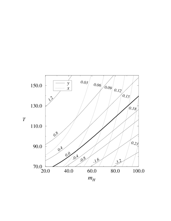
Figure 8: The dimensionless dynamical parameters $x=\bar{\lambda}_{3}/\bar{g}_{3}^{2}$ and $y=\bar{m}_{3}^{2}(\bar{g}_{3}^{2})/\bar{g}_{3}^{4}$ of the 3d SU(2)+Higgs theory as a function of $m_{H}$ and $T$. The parameter $x$ depends on temperature only through logarithmic 1-loop corrections. The tree-level value for the critical temperature $T_{c}$ is given by the line $y=0$, and the true $T_{c}$ is rather close to this line.

Next we go to 2-loop level, which is required for the mass $m_{3}^{2}$. In general, there are three classes of diagrams (see, e.g., Fig. 23 in [23]) contributing at order $g^{4}$: the sunset diagrams, the figure 8 -diagrams, and the 1-loop counterterm diagrams. The counterterm diagrams can contain either the mass or the wave function counterterm. The general strategy is the same as at 1-loop level: from each bosonic diagram, one separates the contribution coming from the $n=0$ modes, since this contribution is reproduced by the 3d theory. The remaining part, analytic in the mass parameters, is not reproduced by the 2-loop diagrams of the 3d theory, and must hence be due to corrections to the tree-level parameters of the 3d theory. The fermionic diagrams do not appear in the 3d theory, but they are IR-safe, and hence directly produce terms analytic in the mass parameters, contributing to $m_{3}^{2}$. We will first give the basic integrals appearing in the calculation, and then the results for the contributions of the superheavy modes to all the different types of diagrams that can appear.

The bosonic tadpole integral is

$$I_{b}(m)={\hbox{$\sum$}\!\!\!\!\!\!\int}_{\!\!\!\!p_{b}}\frac{1}{p^{2}+m^{2}}=I_{b}^{\prime}(m)+I_{3}(m),$$ (72)

where $I^{\prime}_{b}(m)$ is in eq. (32) and the 3d integral is

$$I_{3}(m)=T\int\frac{d^{d}p}{(2\pi)^{d}}\frac{1}{p^{2}+m^{2}}=\mu^{-2\epsilon}\bigg{(}-\frac{mT}{4\pi}\biggr{)}.$$ (73)

The fermionic tadpole integral $I_{f}(m)$ is given in eq. (33). The products appearing in the 2-loop diagrams, apart from inessential vacuum terms, are

$$I_{b}(m_{1})I_{b}(m_{2}) = I_{3}(m_{1})I_{3}(m_{2})+\frac{1}{12}\mu^{-2\epsilon}T^{2}\Bigl{[}I_{3}(m_{1})+I_{3}(m_{2})\Bigr{]}$$ (74)

$$-\mu^{-4\epsilon}\frac{T^{2}}{16\pi^{2}}(m_{1}^{2}+m_{2}^{2})\biggl{(}\frac{1}{12\epsilon}+\frac{L_{b}}{12}+\frac{\imath_{\epsilon}}{12}\biggr{)},$$

$$I_{b}(m)I_{f}(m_{f}) = -\frac{1}{24}\mu^{-2\epsilon}T^{2}I_{3}(m)+\mu^{-4\epsilon}\frac{T^{2}}{16\pi^{2}}\biggl{[}m^{2}\biggl{(}\frac{1}{24\epsilon}+\frac{L_{b}}{24}+\frac{\imath_{\epsilon}}{24}-\frac{1}{12}\ln 2\biggr{)},$$ (75)

$$-m_{f}^{2}\biggl{(}\frac{1}{12\epsilon}+\frac{L_{f}}{12}+\frac{\imath_{\epsilon}}{12}\biggr{)}\biggr{]},$$

$$I_{f}(m_{f})I_{f}(m_{f^{\prime}}) = \mu^{-4\epsilon}\frac{T^{2}}{16\pi^{2}}(m_{f}^{2}+m_{f^{\prime}}^{2})\biggl{(}\frac{1}{24\epsilon}+\frac{L_{f}}{24}+\frac{\imath_{\epsilon}}{24}-\frac{1}{12}\ln 2\biggr{)}.$$ (76)

The bosonic sunset integral is [7, 29]

$$H_{b}(m_{1},m_{2},m_{3}) = {\hbox{$\sum$}\!\!\!\!\!\!\int}_{\!\!\!\!p_{b},q_{b}}\frac{1}{[p^{2}+m_{1}^{2}][q^{2}+m_{2}^{2}][(p+q)^{2}+m_{3}^{2}]}$$ (77)

$$= \mu^{-4\epsilon}\frac{T^{2}}{16\pi^{2}}\biggl{(}\frac{1}{4\epsilon}+\ln\frac{\mu}{m_{1}+m_{2}+m_{3}}+\frac{1}{2}\biggr{)}$$

$$= H_{3}(m_{1},m_{2},m_{3})+\mu^{-4\epsilon}\frac{T^{2}}{16\pi^{2}}\biggl{(}\frac{1}{4}L_{b}+\frac{1}{4}\imath_{\epsilon}+\ln\frac{3T}{\mu}+c\biggr{)},$$

where $H_{3}(m_{1},m_{2},m_{3})$ is the corresponding integral in 3d. Using eq. (31) one can see that the expression in the brackets on the last line actually vanishes, so that $H_{3}(m_{1},m_{2},m_{3})$ is the second line in eq. (77). However, it proves useful to write $H_{b}(m_{1},m_{2},m_{3})$ in the form indicated. The fermionic integral

$$H_{f}(m_{f},m_{f^{\prime}},m) = {\hbox{$\sum$}\!\!\!\!\!\!\int}_{\!\!\!\!p_{f},q_{f}}\frac{1}{[p^{2}+m_{f}^{2}][q^{2}+m_{f^{\prime}}^{2}][(p+q)^{2}+m^{2}]}$$ (78)

vanishes [23].

There is also a third integral, $L(m_{1},m_{2})$, appearing in the 2-loop graphs [23]. Apart from vacuum terms, it is given by

$$L(m_{1},m_{2}) = {\hbox{$\sum$}\!\!\!\!\!\!\int}_{\!\!\!\!p_{b},q_{b}}\frac{(p\cdot q)^{2}}{p^{2}(p^{2}+m_{1}^{2})q^{2}(q^{2}+m_{2}^{2})}$$ (79)

$$= L_{3}(m_{1},m_{2})+\mu^{-2\epsilon}\frac{T^{2}}{24}\Bigl{[}I_{3}(m_{1})+I_{3}(m_{2})\Bigr{]}$$

$$- \mu^{-4\epsilon}\frac{T^{2}}{16\pi^{2}}(m_{1}^{2}+m_{2}^{2})\biggl{(}\frac{1}{48\epsilon}+\frac{L_{b}}{48}+\frac{\imath_{\epsilon}}{48}-\frac{1}{48}\biggr{)},$$

where

$$L_{3}(m_{1},m_{2})=\frac{1}{3}I_{3}(m_{1})I_{3}(m_{2}).$$ (80)

However, this integral does not contribute to the integration over the superheavy scale in the Standard Model, since it is cancelled between the figure 8 and sunset diagrams containing only SU(2) vector fields (${\cal D}_{\rm VV}$ and ${\cal D}_{\rm VVV}$ below) [23].

Using the given integrals and results from [23] for the 2-loop diagrams, one can write down the contributions from the superheavy modes to all the possible types of 2-loop diagrams. We give here explicit results only for the simplest mass combinations in the propagators, relevant for Sec. 4; the results for the cases with other masses can be read by using eqs. (74)-(77) and Appendix A of [23]. As stated above, we need not bother about resummation. The results are

$${\cal D}_{\rm SSS}(m_{1},m_{2},m_{3}) = {\hbox{$\sum$}\!\!\!\!\!\!\int}_{\!\!\!\!p_{b},q_{b}}\frac{1}{[p^{2}+m_{1}^{2}][q^{2}+m_{2}^{2}][(p+q)^{2}+m_{3}^{2}]}$$ (81)

$$= {\cal D}^{3d}_{\rm SSS}+\mu^{-4\epsilon}\frac{T^{2}}{16\pi^{2}}\biggl{(}\frac{L_{b}}{4}+\frac{\imath_{\epsilon}}{4}+\ln\frac{3T}{\mu}+c\biggr{)},$$

$${\cal D}_{\rm SSV}(m_{1},m_{2},M) = {\hbox{$\sum$}\!\!\!\!\!\!\int}_{\!\!\!\!p_{b},q_{b}}\frac{(2p_{\mu}+q_{\mu})(2p_{\nu}+q_{\nu})\Bigl{(}\delta_{\mu\nu}-\frac{q_{\mu}q_{\nu}}{q^{2}}\Bigr{)}}{[p^{2}+m_{1}^{2}][q^{2}+M^{2}][(p+q)^{2}+m_{2}^{2}]}$$ (82)

$$= {\cal D}^{3d}_{\rm SSV}+\frac{1}{6}\mu^{-2\epsilon}T^{2}I_{3}(M)$$

$$+\mu^{-4\epsilon}\frac{T^{2}}{16\pi^{2}}\biggl{[}M^{2}\biggl{(}-\frac{1}{6\epsilon}+\frac{L_{b}}{12}+\frac{\imath_{\epsilon}}{12}+\ln\frac{3T}{\mu}+c\biggr{)}$$

$$-2(m_{1}^{2}+m_{2}^{2})\biggl{(}\frac{L_{b}}{4}+\frac{\imath_{\epsilon}}{4}+\ln\frac{3T}{\mu}+c\biggr{)}\biggr{]},$$

$${\cal D}_{\rm SVV}(m,M,M) = {\hbox{$\sum$}\!\!\!\!\!\!\int}_{\!\!\!\!p_{b},q_{b}}\frac{4\Bigl{(}\delta_{\mu\nu}-\frac{p_{\mu}p_{\nu}}{p^{2}}\Bigr{)}\Bigl{(}\delta_{\mu\nu}-\frac{q_{\mu}q_{\nu}}{q^{2}}\Bigr{)}}{[p^{2}+M^{2}][q^{2}+M^{2}][(p+q)^{2}+m^{2}]}$$ (83)

$$= {\cal D}^{3d}_{\rm SVV}+\mu^{-4\epsilon}\frac{T^{2}}{16\pi^{2}}\biggl{[}\frac{5}{2}L_{b}+\frac{5}{2}\imath_{\epsilon}+10\biggl{(}\ln\frac{3T}{\mu}+c\biggr{)}\biggr{]},$$

$${\cal D}_{\rm VVV}(M,M,M) = \!\!\!\!{\hbox{$\sum$}\!\!\!\!\!\!\int}_{\!\!\!\!p_{b},q_{b}}\!\!\!\frac{\Bigl{(}\delta_{\mu\alpha}-\frac{p_{\mu}p_{\alpha}}{p^{2}}\Bigr{)}\Bigl{(}\delta_{\nu\beta}-\frac{q_{\nu}q_{\beta}}{q^{2}}\Bigr{)}\Bigl{(}\delta_{\rho\gamma}-\frac{r_{\rho}r_{\gamma}}{r^{2}}\Bigr{)}}{[p^{2}+M^{2}][q^{2}+M^{2}][(p+q)^{2}+M^{2}]}F_{\mu\nu\rho}(p,q,r)F_{\alpha\beta\gamma}(p,q,r)$$ (84)

$$= \tilde{\cal D}^{3d}_{\rm VVV}+\frac{7}{4}\mu^{-2\epsilon}T^{2}I_{3}(M)-3L(M,M)$$

$$-\mu^{-4\epsilon}\frac{T^{2}}{16\pi^{2}}M^{2}\biggl{[}\frac{7}{4}\frac{1}{\epsilon}+\frac{31}{4}L_{b}+\frac{31}{4}\imath_{\epsilon}+24\biggl{(}\ln\frac{3T}{\mu}+c\biggr{)}-1\biggr{]},$$

$${\cal D}_{\rm\eta\eta V}(M) = -{\hbox{$\sum$}\!\!\!\!\!\!\int}_{\!\!\!\!p_{b},q_{b}}\frac{p_{\mu}(p_{\nu}+q_{\nu})\Bigl{(}\delta_{\mu\nu}-\frac{q_{\mu}q_{\nu}}{q^{2}}\Bigr{)}}{p^{2}(q^{2}+M^{2})(p+q)^{2}}$$ (85)

$$= {\cal D}^{3d}_{\rm\eta\eta V}-\frac{1}{24}\mu^{-2\epsilon}T^{2}I_{3}(M)$$

$$-\mu^{-4\epsilon}\frac{T^{2}}{16\pi^{2}}M^{2}\biggl{[}-\frac{1}{24\epsilon}+\frac{L_{b}}{48}+\frac{\imath_{\epsilon}}{48}+\frac{1}{4}\biggl{(}\ln\frac{3T}{\mu}+c\biggr{)}\biggr{]},$$

$${\cal D}_{\rm FFS}(m_{f},m_{f^{\prime}},m) = {\hbox{$\sum$}\!\!\!\!\!\!\int}_{\!\!\!\!p_{f},q_{f}}\frac{\mathop{\rm Tr}(i\hbox{$p$}\kern-5.03125pt\hbox to5.03125pt{\hss$\,/$\hss}+m_{f})(i\hbox{$q$}\kern-4.8229pt\hbox to4.8229pt{\hss$\,/$\hss}-m_{f^{\prime}})}{[p^{2}+m_{f}^{2}][q^{2}+m_{f^{\prime}}^{2}][(p+q)^{2}+m^{2}]}$$ (86)

$$= -\frac{1}{6}\mu^{-2\epsilon}T^{2}I_{3}(m)+\mu^{-4\epsilon}\frac{T^{2}}{16\pi^{2}}\biggl{[}m^{2}\biggl{(}\frac{1}{6\epsilon}+\frac{L_{b}}{6}+\frac{\imath_{\epsilon}}{6}-\frac{1}{3}\ln 2\biggr{)}$$

$$-(m_{f}^{2}+m_{f^{\prime}}^{2})\biggl{(}\frac{1}{4\epsilon}+\frac{L_{f}}{4}+\frac{\imath_{\epsilon}}{4}-\frac{1}{6}\ln 2\biggr{)}\biggr{]},$$

$${\cal D}_{\rm FFV}(m_{f},m_{f^{\prime}},M) = -{\hbox{$\sum$}\!\!\!\!\!\!\int}_{\!\!\!\!p_{f},q_{f}}\frac{\mathop{\rm Tr}(i\hbox{$p$}\kern-5.03125pt\hbox to5.03125pt{\hss$\,/$\hss}+m_{f})\gamma_{\mu}a_{L}(i\hbox{$q$}\kern-4.8229pt\hbox to4.8229pt{\hss$\,/$\hss}-m_{f^{\prime}})\gamma_{\nu}a_{L}}{[p^{2}+m_{f}^{2}][q^{2}+m_{f^{\prime}}^{2}][(p+q)^{2}+M^{2}]}\biggl{(}\delta_{\mu\nu}-\frac{r_{\mu}r_{\nu}}{r^{2}}\biggr{)}$$ (87)

$$= -\frac{1}{6}\mu^{-2\epsilon}T^{2}I_{3}(M)+\mu^{-4\epsilon}\frac{T^{2}}{16\pi^{2}}\biggl{[}M^{2}\biggl{(}\frac{1}{6\epsilon}+\frac{L_{b}}{6}+\frac{\imath_{\epsilon}}{6}-\frac{1}{3}\ln 2-\frac{1}{6}\biggr{)}$$

$$-(m_{f}^{2}+m_{f^{\prime}}^{2})\biggl{(}\frac{1}{4\epsilon}+\frac{L_{f}}{4}+\frac{\imath_{\epsilon}}{4}-\frac{1}{6}\ln 2-\frac{1}{4}\biggr{)}\biggr{]},$$

$${\cal D}_{\rm SS}(m_{1},m_{2}) = -{\hbox{$\sum$}\!\!\!\!\!\!\int}_{\!\!\!\!p_{b},q_{b}}\frac{1}{(p^{2}+m_{1}^{2})(q^{2}+m_{2}^{2})}$$ (88)

$$= {\cal D}^{3d}_{\rm SS}-\frac{1}{12}\mu^{-2\epsilon}T^{2}\Bigl{[}I_{3}(m_{1})+I_{3}(m_{2})\Bigr{]}$$

$$+\mu^{-4\epsilon}\frac{T^{2}}{16\pi^{2}}(m_{1}^{2}+m_{2}^{2})\biggl{(}\frac{1}{12\epsilon}+\frac{L_{b}}{12}+\frac{\imath_{\epsilon}}{12}\biggr{)},$$

$${\cal D}_{\rm SV}(m,M) = -2\;{\hbox{$\sum$}\!\!\!\!\!\!\int}_{\!\!\!\!p_{b},q_{b}}\frac{\delta_{\mu\nu}\Bigl{(}\delta_{\mu\nu}-\frac{q_{\mu}q_{\nu}}{q^{2}}\Bigr{)}}{(p^{2}+m^{2})(q^{2}+M^{2})}$$ (89)

$$= {\cal D}^{3d}_{\rm SV}-\frac{1}{2}\mu^{-2\epsilon}T^{2}\Bigl{[}I_{3}(m)+I_{3}(M)\Bigr{]}$$

$$+\mu^{-4\epsilon}\frac{T^{2}}{16\pi^{2}}(m^{2}+M^{2})\biggl{(}\frac{1}{2\epsilon}+\frac{L_{b}}{2}+\frac{\imath_{\epsilon}}{2}-\frac{1}{3}\biggr{)},$$

$${\cal D}_{\rm VV}(M_{1},M_{2}) = -{\hbox{$\sum$}\!\!\!\!\!\!\int}_{\!\!\!\!p_{b},q_{b}}\frac{\Bigl{(}\delta_{\mu\nu}-\frac{p_{\mu}p_{\nu}}{p^{2}}\Bigr{)}\Bigl{(}\delta_{\sigma\rho}-\frac{q_{\sigma}q_{\rho}}{q^{2}}\Bigr{)}}{(p^{2}+M_{1}^{2})(q^{2}+M_{2}^{2})}(2\delta_{\mu\nu}\delta_{\sigma\rho}-\delta_{\mu\sigma}\delta_{\nu\rho}-\delta_{\mu\rho}\delta_{\nu\sigma})$$ (90)

$$= \tilde{\cal D}^{3d}_{\rm VV}-\frac{7}{6}\mu^{-2\epsilon}T^{2}\Bigl{[}I_{3}(M_{1})+I_{3}(M_{2})\Bigr{]}+2L(M_{1},M_{2})$$

$$+\mu^{-4\epsilon}\frac{T^{2}}{16\pi^{2}}(M_{1}^{2}+M_{2}^{2})\biggl{(}\frac{7}{6\epsilon}+\frac{7}{6}L_{b}+\frac{7}{6}\imath_{\epsilon}-\frac{5}{3}\biggr{)},$$

$${\cal D}_{S}(m) = {\hbox{$\sum$}\!\!\!\!\!\!\int}_{\!\!\!\!p_{b}}\frac{\delta m^{2}+\delta Z_{S}p^{2}}{p^{2}+m^{2}}=\mu^{-2\epsilon}\frac{T^{2}}{12}(1+\epsilon\imath_{\epsilon})(\delta m^{2}-m^{2}\delta Z_{S}),$$ (91)

$${\cal D}_{V}(M) = {\hbox{$\sum$}\!\!\!\!\!\!\int}_{\!\!\!\!p_{b}}\frac{\delta M^{2}+\delta Z_{V}p^{2}}{p^{2}+M^{2}}\delta_{\mu\nu}\Bigl{(}\delta_{\mu\nu}-\frac{p_{\mu}p_{\nu}}{p^{2}}\Bigr{)}$$ (92)

$$= \mu^{-2\epsilon}\frac{T^{2}}{12}[3+3\epsilon\imath_{\epsilon}-2\epsilon](\delta M^{2}-M^{2}\delta Z_{V}),$$

$${\cal D}_{F}(m_{f}) = {\hbox{$\sum$}\!\!\!\!\!\!\int}_{\!\!\!\!p_{f}}\frac{1}{p^{2}+m_{f}^{2}}\mathop{\rm Tr}[i\hbox{$p$}\kern-5.03125pt\hbox to5.03125pt{\hss$\,/$\hss}-m_{f}][\delta m_{f}+i\hbox{$p$}\kern-5.03125pt\hbox to5.03125pt{\hss$\,/$\hss}(a_{L}\delta Z^{L}_{F}+a_{R}\delta Z^{R}_{F})]$$ (93)

$$= \mu^{-2\epsilon}\frac{T^{2}}{12}[1+\epsilon(\imath_{\epsilon}-2\ln 2)][\delta m_{f}^{2}-m_{f}^{2}(\delta Z^{L}_{F}+\delta Z^{R}_{F})].$$

In the expressions for ${\cal D}_{\rm VVV}$ and ${\cal D}_{\rm FFV}$, we used $r$ as a shorthand for $-p-q$. The tilde over $\tilde{\cal D}^{3d}_{\rm VVV}$ and $\tilde{\cal D}^{3d}_{\rm VV}$ indicates that the 3d-part of $L(M,M)$ is not included. In eq. (93), $\delta m_{f}^{2}\equiv 2m_{f}\delta m_{f}$.

In addition to the diagrams mentioned above, one may calculate the thermal counterterm diagrams. According to eq. (64), they give contributions of the form

$$-\overline{\Pi}_{\phi}(0)I_{3}(m),\quad-\overline{\Pi}_{A_{0}}(0)I_{3}(M).$$ (94)

These contributions cancel the linear terms proportional to $T^{2}I_{3}(m)$, $T^{2}I_{3}(M)$ in eqs. (81)-(93). After this cancellation, all that is left is terms proportional to the masses squared. Using eq. (65), such terms give the coefficient of $\varphi^{2}/2$, i.e., the mass $m_{3}^{2}$ of the 3d theory. The counterterm contributions ${\cal D}_{S}(m)$, ${\cal D}_{V}(M)$, ${\cal D}_{F}(m_{f})$ do not cancel all the $1/\epsilon$-parts from the other contributions, since there remains a 2-loop mass counterterm in the 3d theory [7].

3.1.5 The couplings of the adjoint scalar sector

The couplings of the adjoint scalar sector could be calculated from an effective potential as for the fundamental scalar sector, but for completeness we calculate them directly from Feynman diagrams. We make here just a 1-loop calculation.

The 1-loop diagrams needed for calculating the $(A_{0}A_{0})$-correlator at vanishing external momenta are shown in Fig. 4. We need two new integrals, obtained by taking the derivative of eqs. (32), (33) with respect to $T$. With the accuracy needed,

$$E_{b}^{\prime}(m) = {\hbox{$\sum$}\!\!\!\!\!\!\int}_{\!\!\!\!p_{b}}^{\prime}\frac{p_{0}^{2}}{(p^{2}+m^{2})^{2}}=-\frac{T^{2}}{24}-\frac{m^{2}}{16\pi^{2}}\biggl{(}\frac{1}{2\epsilon_{b}}+1\biggr{)},$$

$$E_{f}(m) = {\hbox{$\sum$}\!\!\!\!\!\!\int}_{\!\!\!\!p_{f}}\frac{p_{0}^{2}}{(p^{2}+m^{2})^{2}}=\frac{T^{2}}{48}-\frac{m^{2}}{16\pi^{2}}\biggl{(}\frac{1}{2\epsilon_{f}}+1\biggr{)}.$$ (95)

Note that $E_{b}^{\prime}(0)$ is the constant part subtracted in the definition of $J^{b}_{00}$ in eq. (34). Using the integrals in eq. (95) together with those in eqs. (32), (34), the diagrams in Fig. 4 give

$${\cal A}^{(2)}_{\rm S} = {\hbox{$\sum$}\!\!\!\!\!\!\int}_{\!\!\!\!p_{b}}^{\prime}\frac{1}{p^{2}+m_{S}^{2}}=I_{b}^{\prime}(m_{S})=\frac{T^{2}}{12}-\frac{m_{S}^{2}}{16\pi^{2}}\frac{1}{\epsilon_{b}},$$ (96)

$${\cal A}^{(2)}_{\rm V} = {\hbox{$\sum$}\!\!\!\!\!\!\int}_{\!\!\!\!p_{b}}^{\prime}\frac{\delta_{\mu\nu}-\frac{p_{\mu}p_{\nu}}{p^{2}}}{p^{2}}\Bigl{(}2\delta_{00}\delta_{\mu\nu}-2\delta_{0\mu}\delta_{0\nu}\Bigr{)}=4(1-\epsilon)I_{b}^{\prime}(0)+2E_{b}^{\prime}(0)=\frac{T^{2}}{4},$$ (97)

$${\cal A}^{(2)}_{\rm SS} = {\hbox{$\sum$}\!\!\!\!\!\!\int}_{\!\!\!\!p_{b}}^{\prime}\frac{(2p_{0})^{2}}{(p^{2}+m_{S}^{2})^{2}}=4E_{b}^{\prime}(m_{S})=-\frac{T^{2}}{6}-\frac{m_{S}^{2}}{16\pi^{2}}\biggl{(}\frac{2}{\epsilon_{b}}+4\biggr{)},$$ (98)

$${\cal A}^{(2)}_{\rm VV} = {\hbox{$\sum$}\!\!\!\!\!\!\int}_{\!\!\!\!p_{b}}^{\prime}\frac{(12-8\epsilon)p_{0}^{2}}{(p^{2})^{2}}=(12-8\epsilon)E_{b}^{\prime}(0)=-\frac{T^{2}}{2},$$ (99)

$${\cal A}^{(2)}_{\eta\eta} = {\hbox{$\sum$}\!\!\!\!\!\!\int}_{\!\!\!\!p_{b}}^{\prime}\frac{p_{0}^{2}}{(p^{2})^{2}}=E_{b}^{\prime}(0)=-\frac{T^{2}}{24},$$ (100)

$${\cal A}^{(2)}_{\rm FF} = -2{\hbox{$\sum$}\!\!\!\!\!\!\int}_{\!\!\!\!p_{f}}\frac{2p_{0}^{2}-p^{2}}{(p^{2})^{2}}=-4E_{f}(0)+2I_{f}(0)=-\frac{T^{2}}{6}.$$ (101)

For ${\cal A}^{(2)}_{\rm SS}$, ${\cal A}^{(2)}_{\rm VV}$, ${\cal A}^{(2)}_{\rm\eta\eta}$, and ${\cal A}^{(2)}_{\rm FF}$, the integrand was obtained from eqs. (40), (47), (42), and (44) by putting $k\to 0$. In the final result, the $1/\epsilon$-parts cancel between ${\cal A}^{(2)}_{\rm S}$ and ${\cal A}^{(2)}_{\rm SS}$. The constant term proportional to $m_{S}^{2}$ is of higher order, and the $T^{2}$-terms give the desired 3d mass parameter.

The diagrams needed for the $(A_{0}A_{0}A_{0}A_{0})$-correlator are shown in Fig. 5. They give

$${\cal A}^{(4)}_{\rm SS} = {\hbox{$\sum$}\!\!\!\!\!\!\int}_{\!\!\!\!p_{b}}^{\prime}\frac{1}{(p^{2})^{2}}=B_{b}^{\prime}=\frac{1}{16\pi^{2}}\frac{1}{\epsilon_{b}},$$ (102)

$${\cal A}^{(4)}_{\rm SSS} = {\hbox{$\sum$}\!\!\!\!\!\!\int}_{\!\!\!\!p_{b}}^{\prime}\frac{(2p_{0})^{2}}{(p^{2})^{3}}=4K^{b}_{00}=\frac{1}{16\pi^{2}}\biggl{(}\frac{1}{\epsilon_{b}}+2\biggr{)},$$ (103)

$${\cal A}^{(4)}_{\rm SSSS} = {\hbox{$\sum$}\!\!\!\!\!\!\int}_{\!\!\!\!p_{b}}^{\prime}\frac{(2p_{0})^{4}}{(p^{2})^{4}}=16L^{b}_{0}=\frac{1}{16\pi^{2}}\biggl{(}\frac{2}{\epsilon_{b}}+\frac{16}{3}\biggr{)},$$ (104)

$${\cal A}^{(4)}_{\rm VV} = {\hbox{$\sum$}\!\!\!\!\!\!\int}_{\!\!\!\!p_{b}}^{\prime}\frac{\Bigl{(}\delta_{\mu\nu}-\frac{p_{\mu}p_{\nu}}{p^{2}}\Bigr{)}\Bigl{(}\delta_{\sigma\rho}-\frac{p_{\sigma}p_{\rho}}{p^{2}}\Bigr{)}}{(p^{2})^{2}}$$ (105)

$$\times\Bigl{(}2\delta_{00}\delta_{\mu\sigma}-2\delta_{0\mu}\delta_{0\sigma}\Bigr{)}\Bigl{(}2\delta_{00}\delta_{\nu\rho}-2\delta_{0\nu}\delta_{0\rho}\Bigr{)}$$

$$= 8(1-\epsilon)B_{b}^{\prime}+4L^{b}_{0}=\frac{1}{16\pi^{2}}\biggl{(}\frac{17}{2}\frac{1}{\epsilon_{b}}-\frac{20}{3}\biggr{)},$$

$${\cal A}^{(4)}_{\rm VVV} = {\hbox{$\sum$}\!\!\!\!\!\!\int}_{\!\!\!\!p_{b}}^{\prime}\frac{\Bigl{(}\delta_{\mu\nu}-\frac{p_{\mu}p_{\nu}}{p^{2}}\Bigr{)}\Bigl{(}\delta_{\sigma\alpha}-\frac{p_{\sigma}p_{\alpha}}{p^{2}}\Bigr{)}\Bigl{(}\delta_{\rho\beta}-\frac{p_{\rho}p_{\beta}}{p^{2}}\Bigr{)}}{(p^{2})^{3}}$$ (106)

$$\times F_{0\mu\sigma}(0,p,-p)F_{0\nu\rho}(0,p,-p)\Bigl{(}2\delta_{00}\delta_{\alpha\beta}-2\delta_{0\alpha}\delta_{0\beta}\Bigr{)}$$

$$= 16(1-\epsilon)K^{b}_{00}+8L^{b}_{0}=\frac{1}{16\pi^{2}}\biggl{(}\frac{5}{\epsilon_{b}}+\frac{20}{3}\biggr{)},$$

$${\cal A}^{(4)}_{\rm VVVV} = {\hbox{$\sum$}\!\!\!\!\!\!\int}_{\!\!\!\!p_{b}}^{\prime}\frac{\Bigl{(}\delta_{\alpha\beta}-\frac{p_{\alpha}p_{\beta}}{p^{2}}\Bigr{)}\Bigl{(}\delta_{\gamma\delta}-\frac{p_{\gamma}p_{\delta}}{p^{2}}\Bigr{)}\Bigl{(}\delta_{\mu\nu}-\frac{p_{\mu}p_{\nu}}{p^{2}}\Bigr{)}\Bigl{(}\delta_{\sigma\rho}-\frac{p_{\sigma}p_{\rho}}{p^{2}}\Bigr{)}}{(p^{2})^{4}}$$ (107)

$$\times F_{0\alpha\gamma}(0,p,-p)F_{0\delta\nu}(0,p,-p)F_{0\mu\sigma}(0,p,-p)F_{0\beta\rho}(0,p,-p)$$

$$= 16(3-2\epsilon)L^{b}_{0}=\frac{1}{16\pi^{2}}\biggl{(}\frac{6}{\epsilon_{b}}+12\biggr{)},$$

$${\cal A}^{(4)}_{\rm\eta\eta\eta\eta} = {\hbox{$\sum$}\!\!\!\!\!\!\int}_{\!\!\!\!p_{b}}^{\prime}\frac{p_{0}^{4}}{(p^{2})^{4}}=L^{b}_{0}=\frac{1}{16\pi^{2}}\biggl{(}\frac{1}{8\epsilon_{b}}+\frac{1}{3}\biggr{)},$$ (108)

$${\cal A}^{(4)}_{\rm FFFF} = {\hbox{$\sum$}\!\!\!\!\!\!\int}_{\!\!\!\!p_{f}}\frac{1}{(p^{2})^{4}}\mathop{\rm Tr}[(i\hbox{$p$}\kern-5.03125pt\hbox to5.03125pt{\hss$\,/$\hss}\gamma_{0}a_{L})(i\hbox{$p$}\kern-5.03125pt\hbox to5.03125pt{\hss$\,/$\hss}\gamma_{0}a_{L})(i\hbox{$p$}\kern-5.03125pt\hbox to5.03125pt{\hss$\,/$\hss}\gamma_{0}a_{L})(i\hbox{$p$}\kern-5.03125pt\hbox to5.03125pt{\hss$\,/$\hss}\gamma_{0}a_{L})]$$ (109)

$$= =16L^{f}_{0}-16K^{f}_{00}+2B_{f}^{\prime}=\frac{1}{16\pi^{2}}\biggl{(}-\frac{8}{3}\biggr{)}.$$

Again the $1/\epsilon$-parts cancel when the correct coefficients are included, since there are no coupling constant counterterms in the 3d theory.

3.2 Integration over the heavy scale

The integration over the heavy scale proceeds analogously to the integration over the superheavy scale. Instead of an infinite number of excitations with masses $\sim\pi T$, there are now a finite number of fields with masses $m_{D}\sim gT$. The heavy fields include, in particular, the temporal components $A_{0}$ of the gauge fields. The heavy fields are scalars in the effective 3d theory, so no gauge fixing is needed for the integration. The general form of the resulting theory differs from the starting point only by the absence of the heavy fields, so that the final theory is the light bosonic sector of the original 4d theory, but in three spatial dimensions.

There are three kinds of vertices which the heavy field $A_{0}$ feels. The interactions with the spatial gauge fields follow from eq. (25), and are of the form

$$ig_{3}f^{abc}A_{0}^{a}(p)A_{i}^{b}(q)A_{0}^{c}(r)(p_{i}-r_{i}),\quad g_{3}^{2}G^{abcd}_{ij00}A^{a}_{i}A^{b}_{j}A^{c}_{0}A^{d}_{0},$$ (110)

where $G^{abcd}_{ij00}\propto\delta_{ij}$. Here $g_{3}$ denotes the dimensionful 3d gauge coupling, and the fields have also been scaled by $T$ to have the dimension GeV^1/2. In addition to eq. (110) there are different quartic scalar vertices. One of the scalar vertices, the quartic self-interaction of $A_{0}$, can be neglected, since the coupling constant is of order $g^{4}$, and would appear only inside 2-loop graphs where it is further suppressed by other couplings.

The integration measure in 3d is denoted by

$$\int dp\equiv\int\frac{d^{d}p}{(2\pi)^{d}}.$$ (111)

The $A_{0}$-propagator in the symmetric phase is

$$\langle A_{0}(p)A_{0}(-p)\rangle=\frac{1}{p^{2}+m_{D}^{2}}.$$ (112)

The basic integrals needed are $\bar{I}_{3}(m)$, which is just eq. (73) without $T$, together with ${\cal B}(k^{2};m_{1},m_{2})$ and ${\cal J}_{ij}$, defined by

$${\cal B}(k^{2};m_{1},m_{2}) = \int dp\frac{1}{[p^{2}+m_{1}^{2}][(p+k)^{2}+m_{2}^{2}]}$$ (113)

$$= \frac{i}{8\pi(k^{2})^{1/2}}\ln\frac{m_{1}+m_{2}-i(k^{2})^{1/2}}{m_{1}+m_{2}+i(k^{2})^{1/2}}$$

$$= \frac{1}{4\pi(m_{1}+m_{2})}\biggl{[}1-\frac{1}{3}\frac{k^{2}}{(m_{1}+m_{2})^{2}}+\ldots\biggr{]},$$

$${\cal J}_{ij} = \int dp\frac{p_{i}p_{j}}{[p^{2}+m_{D}^{2}][(p+k)^{2}+m_{D}^{2}]}-\int dp\frac{p_{i}p_{j}}{(p^{2}+m_{D}^{2})^{2}}$$ (114)

$$= -\biggl{(}\delta_{ij}-\frac{k_{i}k_{j}}{k^{2}}\biggr{)}\frac{k^{2}}{96\pi m_{D}}+\frac{k_{i}k_{j}}{32\pi m_{D}}+{\cal O}\Bigl{(}\frac{k^{4}}{m_{D}^{3}}\Bigr{)}.$$

Using these integrals, the task is to calculate the corrections from $m_{D}$ to the parameters of the final theory in powers of $g_{3}^{2}/m_{D}$, where it is assumed that the light masses and momenta are $m\sim k\sim g_{3}^{2}$.

Let us start with wave function normalization. Since the fundamental scalar field interacts with $A_{0}$ only through quartic vertices, there is no momentum-dependent correction from the $A_{0}$-field to the $\phi$-correlator. Hence the normalization of $\phi$ does not change. The momentum-dependent correction to the $A_{i}$-correlator comes from the diagram with two internal $A_{0}$-propagators, and is, in analogy with ${\cal Z}^{A_{i}}_{\rm SS}$ in eq. (41),

$${\cal Z}^{A_{i}}_{\rm LL} = \int dp\frac{(2p_{i}+k_{i})(2p_{j}+k_{j})}{[p^{2}+m_{D}^{2}][(p+k)^{2}+m_{D}^{2}]}$$ (115)

$$\Rightarrow 4{\cal J}^{(T)}_{ij}=-\biggl{(}\delta_{ij}-\frac{k_{i}k_{j}}{k^{2}}\biggr{)}\frac{k^{2}}{24\pi m_{D}}.$$

The heavy propagators are denoted by L.

To fix the gauge coupling, one can calculate the contributions of $A_{0}$ to the $(\phi\phi A_{i}A_{j})$-vertex. There are two types of diagrams, in analogy with ${\cal G}^{A_{i}}_{\rm SS}$ and ${\cal G}^{A_{i}}_{\rm SSS}$ in eqs. (53), (59). The contributions are

$${\cal G}_{\rm LL} = \int dp\frac{\delta_{ij}}{(p^{2}+m_{D}^{2})^{2}}=\frac{\delta_{ij}}{8\pi m_{D}},$$ (116)

$${\cal G}_{\rm LLL} = \int dp\frac{(2p_{i})(2p_{j})}{(p^{2}+m_{D}^{2})^{3}}=\frac{\delta_{ij}}{8\pi m_{D}}.$$ (117)

It is very easy to calculate the 1-loop corrections to the parameters of the scalar sector, since the field one is integrating over is itself a scalar. Hence the diagrams can give just $\bar{I}_{3}(m_{D})$ or ${\cal B}(0;m_{D},m_{D})$. For the mass parameter, one needs again a 2-loop calculation, and it is best to employ the effective potential. After the shift, the mass of the heavy field is of the form $m_{L}^{2}=m_{D}^{2}+h_{3}\varphi^{2}$, where $h_{3}$ is the coupling of the $(\phi\phi A_{0}A_{0})$-interaction. The diagrams with heavy fields in internal lines do not exist in the final theory, so their effect has to be produced by different parameters in the action. One needs to expand the results of these diagrams in powers of $m/m_{D}$ to such order that terms of the form $m_{D}m$ and $m^{2}$ are kept. Constant terms proportional to $m_{D}^{2}$ ar neglected. For the expansion, one writes

$$m_{L}=m_{D}+\frac{1}{2}\frac{h_{3}\varphi^{2}}{m_{D}}+\ldots\,.$$ (118)

There are four types of possible 2-loop diagrams, and they give [7]

$$D_{\rm LS}(m) = \int dp\,dq\frac{1}{(p^{2}+m_{L}^{2})(q^{2}+m^{2})}$$ (119)

$$= \bar{I}_{3}(m_{L})\bar{I}_{3}(m)\Rightarrow-\frac{\mu^{-2\epsilon}}{4\pi}m_{D}\bar{I}_{3}(m),$$

$$D_{\rm LV}(M) = \int dp\,dq\frac{\delta_{ij}\Bigl{(}\delta_{ij}-\frac{q_{i}q_{j}}{q^{2}}\Bigr{)}}{(p^{2}+m_{L}^{2})(q^{2}+M^{2})}$$ (120)

$$= (2-2\epsilon)\bar{I}_{3}(m_{L})\bar{I}_{3}(M)\Rightarrow-\frac{\mu^{-2\epsilon}}{2\pi}m_{D}\bar{I}_{3}(M),$$

$$D_{\rm LLS}(m) = \int dp\,dq\frac{1}{[p^{2}+m_{L}^{2}][q^{2}+m_{L}^{2}][(p+q)^{2}+m^{2}]}$$ (121)

$$= \bar{H}_{3}(m_{L},m_{L},m)\Rightarrow\frac{\mu^{-4\epsilon}}{16\pi^{2}}\biggl{(}\frac{1}{4\epsilon}+\ln\frac{\mu}{2m_{D}}+\frac{1}{2}\biggr{)},$$

$$D_{\rm LLV}(M) = \int dp\,dq\frac{(2p_{i}+q_{i})(2p_{j}+q_{j})\Bigl{(}\delta_{ij}-\frac{q_{i}q_{j}}{q^{2}}\Bigr{)}}{[p^{2}+m_{L}^{2}][q^{2}+M^{2}][(p+q)^{2}+m_{L}^{2}]}$$ (122)

$$= (M^{2}-4m_{L}^{2})\bar{H}_{3}(m_{L},m_{L},M)+2\bar{I}_{3}(m_{L})\bar{I}_{3}(M)-\bar{I}_{3}(m_{L})\bar{I}_{3}(m_{L})$$

$$\Rightarrow -\frac{\mu^{-2\epsilon}}{\pi}m_{D}\bar{I}_{3}(M)$$

$$+\frac{\mu^{-4\epsilon}}{16\pi^{2}}\biggl{[}M^{2}\biggl{(}\frac{1}{4\epsilon}+\ln\frac{\mu}{2m_{D}}\biggr{)}-h_{3}\varphi^{2}\biggl{(}\frac{1}{\epsilon}+4\ln\frac{\mu}{2m_{D}}+1\biggr{)}\biggr{]}.$$

Here $\bar{H}_{3}$ is the $H_{3}$ of eq. (77) divided by $T^{2}$. The “linear” terms proportional to $m_{D}\bar{I}_{3}(m)$ in $D_{\rm LV}$ and $D_{\rm LLV}$ cancel each other, and those in $D_{\rm LS}$ are cancelled by corrections from $m_{D}$ to the mass of the scalar field inside 1-loop diagrams. This is in complete analogy with the cancellation of linear terms in the integration over the superheavy scale by the thermal counterterms. The actual effect then comes from the diagrams $D_{\rm LLS}$ and $D_{\rm LLV}$. The $1/\epsilon$-parts account for the change in the mass counterterm, and the rest gives the change in the renormalized mass parameter.

4 Dimensional reduction in the Standard Model

In this Section we add the correct coefficients, relevant for the Standard Model, to the generic results of Sec. 3. The coefficients are composed of combinatorial factors, group theoretic factors from isospin contractions, and of coupling constants. We also explain in detail how the final 3d theory is constructed.

4.1 Notation

We treat the Standard Model with the Higgs sector

$${\cal L}_{s}=(D_{\mu}\Phi)^{\dagger}D_{\mu}\Phi-\nu^{2}\Phi^{\dagger}\Phi+\lambda\Bigl{(}\Phi^{\dagger}\Phi\Bigr{)}^{2}$$ (123)

in the following consistent approximation. We take $g_{Y}\neq 0$ only for the top quark, so that the Yukawa sector is

$${\cal L}_{Y}=g_{Y}\bigl{(}\bar{q}_{L}\tilde{\Phi}t_{R}+\bar{t}_{R}\tilde{\Phi}^{\dagger}q_{L}\bigr{)}.$$ (124)

Here $\tilde{\Phi}=i\tau_{2}\Phi^{*}$, $\tau_{2}$ is a Pauli matrix, and $\Phi$ is the Higgs doublet. The gauge couplings are denoted by $g$, $g^{\prime}$, and $g_{S}$. We use the formal power-counting rule $g^{\prime 2}\sim g^{3}$, and keep contributions only below order $g^{5}$. This allows one to neglect $g^{\prime 2}$ e.g. inside 1-loop formulas of vacuum renormalization, so that $m_{W}=m_{Z}$ there.

Most of the counterterms of the Standard Model can be read from eq. (A11) of [23]. For completeness, let us state the bare parameters of the Higgs sector, since the terms proportional to $\lambda$ were neglected in [23]:

$$\lambda_{B} = \lambda+\frac{\mu^{-2\epsilon}}{(4\pi)^{2}\epsilon}\biggl{(}\frac{9}{16}g^{4}-\frac{9}{2}\lambda g^{2}+12\lambda^{2}-3g_{Y}^{4}+6\lambda g_{Y}^{2}\biggr{)},$$ (125)

$${\nu}^{2}_{B} = \nu^{2}\biggl{[}1-\frac{\mu^{-2\epsilon}}{(4\pi)^{2}\epsilon}\biggl{(}\frac{9}{4}g^{2}-6\lambda-3g_{Y}^{2}\biggr{)}\biggr{]}.$$ (126)

Here the coupling constants have not been scaled to be dimensionless in contrast to [23]. Note that our convention for $\lambda$ differs from [23] additionally by the factor 6. Let us also write down a few useful combinations of the bare parameters:

$$\nu^{2}_{B}\phi_{B}^{2} = \nu^{2}\phi^{2}\biggl{[}1+\frac{\mu^{-2\epsilon}}{(4\pi)^{2}\epsilon}6\lambda\biggr{]},$$ (127)

$$\lambda_{B}\phi_{B}^{4} = \phi^{4}\biggl{[}\lambda+\frac{\mu^{-2\epsilon}}{(4\pi)^{2}\epsilon}\biggl{(}\frac{9}{16}g^{4}+12\lambda^{2}-3g_{Y}^{4}\biggr{)}\biggr{]},$$ (128)

$$g_{B}^{2}\phi_{B}^{2}A_{B}^{2} = g^{2}\phi^{2}A^{2}\biggl{[}1-\frac{\mu^{-2\epsilon}}{(4\pi)^{2}\epsilon}\biggl{(}\frac{3}{4}g^{2}+3g_{Y}^{2}\biggr{)}\biggr{]},$$ (129)

$$g_{Y,B}\bar{q}_{L,B}\tilde{\Phi}_{B}t_{R,B} = g_{Y}\bar{q}_{L}\tilde{\Phi}t_{R}\biggl{[}1-\frac{\mu^{-2\epsilon}}{(4\pi)^{2}\epsilon}4g_{S}^{2}\biggr{]}.$$ (130)

Within our approximation, the Standard Model contains five running parameters, $\nu^{2}(\mu)$, $g^{2}(\mu)$, $\lambda(\mu)$, $g_{Y}^{2}(\mu)$, and $g_{S}^{2}(\mu)$. The first four run at 1-loop order as

$$\mu\frac{d}{d\mu}\nu^{2}(\mu) = \frac{1}{8\pi^{2}}\biggl{(}-\frac{9}{4}g^{2}+6\lambda+3g_{Y}^{2}\biggr{)}\nu^{2},$$ (131)

$$\mu\frac{d}{d\mu}g^{2}(\mu) = \frac{1}{8\pi^{2}}\biggl{(}\frac{8n_{F}+N_{s}-44}{6}\biggr{)}g^{4},$$ (132)

$$\mu\frac{d}{d\mu}\lambda(\mu) = \frac{1}{8\pi^{2}}\biggl{(}\frac{9}{16}g^{4}-\frac{9}{2}\lambda g^{2}+12\lambda^{2}-3g_{Y}^{4}+6\lambda g_{Y}^{2}\biggr{)},$$ (133)

$$\mu\frac{d}{d\mu}g_{Y}^{2}(\mu) = \frac{1}{8\pi^{2}}\biggl{(}\frac{9}{2}g_{Y}^{4}-\frac{9}{4}g^{2}g_{Y}^{2}-8g_{S}^{2}g_{Y}^{2}\biggr{)}.$$ (134)

Here $n_{F}=3$ is the number of families and $N_{s}=1$ is the number of Higgs doublets. The running of the strong coupling $g_{S}$ is not explicitly needed for the present problem, since $g_{S}$ appears only inside loop corrections. The running of $g^{\prime 2}$ is of higher order according to our convention. The fields $\Phi$, $A$ and $\psi$ run as well, and the formulas can be extracted, e.g., from eqs. (127)-(130), (131)-(134).

To simplify some of the formulas below, we will use extensively the notation

$$h\equiv\frac{m_{H}}{m_{W}},\quad t\equiv\frac{m_{t}}{m_{W}},\quad s\equiv\frac{g_{S}}{g},$$ (135)

where $m_{W}$, $m_{H}$ and $m_{t}$ are the physical W boson, Higgs particle and top quark masses. Inside 1-loop formulas one may use the tree level relations $g^{2}h^{2}=8\lambda$ and $g^{2}t^{2}=2g_{Y}^{2}$.

4.2 Integration over the superheavy scale

For the SU(2)+Higgs model, the formulas for dimensional reduction to order $g^{4}$ have been given in [7]. We add here the effect of fermions, and correct an error coming from [6].

Due to 3d gauge invariance, the effective 3d theory is of the form

$$S = \int\!d^{3}x\biggl{\{}\frac{1}{4}G^{a}_{ij}G^{a}_{ij}+\frac{1}{4}F_{ij}F_{ij}+(D_{i}\Phi)^{\dagger}(D_{i}\Phi)+m_{3}^{2}\Phi^{\dagger}\Phi+\lambda_{3}(\Phi^{\dagger}\Phi)^{2}$$ (136)

$$\hskip 28.45274pt+\frac{1}{2}(D_{i}A_{0}^{a})^{2}+\frac{1}{2}m_{D}^{2}A_{0}^{a}A_{0}^{a}+\frac{1}{4}\lambda_{A}(A_{0}^{a}A_{0}^{a})^{2}+\frac{1}{2}(\partial_{i}B_{0})^{2}+\frac{1}{2}m_{D}^{\prime 2}B_{0}B_{0}$$

$$\hskip 28.45274pt+h_{3}\Phi^{\dagger}\Phi A_{0}^{a}A_{0}^{a}+h_{3}^{\prime}\Phi^{\dagger}\Phi B_{0}B_{0}-\frac{1}{2}g_{3}g_{3}^{\prime}B_{0}\Phi^{\dagger}A_{0}^{a}\tau^{a}\Phi\,\,\biggr{\}},$$

where $G^{a}_{ij}=\partial_{i}A_{j}^{a}-\partial_{j}A_{i}^{a}+g_{3}\epsilon^{abc}A^{b}_{i}A^{c}_{j}$, $F_{ij}=\partial_{i}B_{j}-\partial_{j}B_{i}$, $D_{i}\Phi=(\partial_{i}-ig_{3}\tau^{a}A^{a}_{i}/2+ig_{3}^{\prime}B_{i}/2)\Phi$, $D_{i}A_{0}^{a}=\partial_{i}A_{0}^{a}+g_{3}\epsilon^{abc}A_{i}^{b}A_{0}^{c}$, and $\Phi=(\phi_{3}+i\phi_{4},\phi_{1}+i\phi_{2})^{T}/\sqrt{2}$. The $\tau^{a}$:s are the Pauli matrices. The factor $1/T$ multiplying the action has been scaled into the fields and the coupling constants, so that the fields have the dimension GeV^1/2 and the couplings $g_{3}^{2}$, $\lambda_{3}$ have the dimension GeV. Due to the convention $g^{\prime 2}\sim g^{3}$, we can use $h_{3}^{\prime}=g_{3}^{\prime 2}/4$, neglect the quartic coupling of $B_{0}$-fields, and use the indicated tree-level values $g_{3}$, $g_{3}^{\prime}$ in the part mixing $A_{0}$ and $B_{0}$. The problem is to calculate the parameters in eq. (136) to order $g^{4}$ in the coupling constants.

First, let us calculate how the 3d fields are related to the 4d fields. The momentum-dependent contribution of the superheavy modes to the two-point scalar correlator is

$${\cal Z}^{\phi}={\cal Z}^{\phi}_{\rm CT}-\frac{3}{4}g^{2}{\cal Z}^{\phi}_{\rm SV}+\frac{3}{2}g_{Y}^{2}{\cal Z}^{\phi}_{\rm FF}=\frac{k^{2}}{16\pi^{2}}(-\frac{9}{4}g^{2}L_{b}+3g_{Y}^{2}L_{f}),$$ (137)

where the ${\cal Z}^{\phi}$’s are from eqs. (35)-(37). For the spatial and temporal components of the gauge fields one gets

$${\cal Z}^{A}={\cal Z}^{A}_{\rm CT}-\frac{N_{s}}{2}g^{2}{\cal Z}^{A}_{\rm SS}+2g^{2}{\cal Z}^{A}_{\eta\eta}-2n_{F}g^{2}{\cal Z}^{A}_{\rm FF}-g^{2}{\cal Z}^{A}_{\rm VV},$$ (138)

where the ${\cal Z}^{A}$’s are from eqs. (38)-(49). This gives

$${\cal Z}^{A_{0}} = \frac{g^{2}k^{2}}{16\pi^{2}}\biggl{[}\frac{4n_{F}}{3}(L_{f}-1)+\frac{N_{s}}{6}(L_{b}+2)-\frac{13}{3}L_{b}+\frac{8}{3}\biggr{]},$$ (139)

$${\cal Z}^{A_{i}} = \biggl{(}\delta_{ij}-\frac{k_{i}k_{j}}{k^{2}}\biggr{)}\frac{g^{2}k^{2}}{16\pi^{2}}\biggl{[}\frac{4n_{F}}{3}L_{f}+\frac{N_{s}}{6}L_{b}-\frac{13}{3}L_{b}-\frac{2}{3}\biggr{]}.$$ (140)

The $\cal Z$’s here correspond just to $\overline{\Pi}^{\prime}(0)k^{2}$ in eq. (14). Hence the wave functions in the 3d action are related to the renormalized 4d wave functions in the $\overline{\rm MS}$-scheme by

$$\phi_{3}^{2} = \frac{1}{T}\phi^{2}\biggl{\{}1+\frac{1}{16\pi^{2}}\biggl{[}-\frac{9}{4}g^{2}L_{b}+3g_{Y}^{2}L_{f}\biggr{]}\biggr{\}},$$ (141)

$$\bigl{(}A_{0}^{3d}\bigr{)}^{2} = \frac{1}{T}\bigl{(}A_{0}\bigr{)}^{2}\biggl{\{}1+\frac{g^{2}}{16\pi^{2}}\biggl{[}\frac{4n_{F}}{3}(L_{f}-1)+\frac{N_{s}}{6}(L_{b}+2)-\frac{13}{3}L_{b}+\frac{8}{3}\biggr{]}\biggr{\}},$$ (142)

$$\bigl{(}A_{i}^{3d}\bigr{)}^{2} = \frac{1}{T}\bigl{(}A_{i}\bigr{)}^{2}\biggl{\{}1+\frac{g^{2}}{16\pi^{2}}\biggl{[}\frac{4n_{F}}{3}L_{f}+\frac{N_{s}}{6}L_{b}-\frac{13}{3}L_{b}-\frac{2}{3}\biggr{]}\biggr{\}}.$$ (143)

The factor $1/T$ arises because of the rescaling in eq. (136). The loop corrections to the normalization of $B_{0}$ are of higher order according to our convention. When the running of fields in 4d is taken into account, $\phi_{3}$, $A_{0}^{3d}$ and $A_{i}^{3d}$ are seen to be independent of $\mu$.

The constant $-2/3$ inside the square brackets in the formulas for $A_{0}^{3d}$ and $A_{i}^{3d}$ in eqs. (142), (143) is missing in [7], due to an error in eq. (6.3) in [6]. This error propagates to $g_{3}^{2}$ and $h_{3}$; the correct result for $g_{3}^{2}$ is also given in eq. (6) of [18].

Second, let us calculate the 1-loop corrections to the coupling constants of the gauge sector. The couplings $g_{3}^{2}$ and $h_{3}$ can be extracted from the $n\neq 0$ contributions to the $(\phi\phi A_{i}A_{j})$- and $(\phi\phi A_{0}A_{0})$-correlators at vanishing external momenta, respectively. The corrections to the $(\phi\phi BB)$- and $(\phi\phi B_{0}A_{0})$-vertices are of higher order. The contributions from the relevant diagrams are in eqs. (50)-(63). The coefficients are such that

$${\cal G}^{A} = {\cal G}^{A}_{0}+{\cal G}^{A}_{\rm CT}-6\lambda g^{2}{\cal G}^{A}_{\rm SS}-g^{4}{\cal G}^{A}_{\rm SV}-g^{4}{\cal G}^{A}_{\rm VV}$$ (144)

$$+6\lambda g^{2}{\cal G}^{A}_{\rm SSS}+2g^{4}{\cal G}^{A}_{\rm VVV}-3g^{2}g_{Y}^{2}{\cal G}^{A}_{\rm FFFF}.$$

This gives the effective vertices

$$\frac{g^{2}}{8}\phi_{i}\phi_{i}A^{a}_{j}A^{a}_{j}\biggl{[}1+\frac{1}{16\pi^{2}}\biggl{(}\frac{3}{4}g^{2}L_{b}+3g_{Y}^{2}L_{f}\biggr{)}\biggr{]},$$

$$\frac{g^{2}}{8}\phi_{i}\phi_{i}A^{a}_{0}A^{a}_{0}\biggl{[}1+\frac{1}{16\pi^{2}}\biggl{(}\frac{3}{4}g^{2}L_{b}+3g_{Y}^{2}L_{f}+\frac{23}{2}g^{2}+12\lambda-6g_{Y}^{2}\biggr{)}\biggr{]},$$ (145)

where the fields are those of the 4d theory. When the fields are redefined according to eqs. (141)-(143) and the vertex is identified with the corresponding vertex in eq. (136), one gets the final result for the coupling constants $g_{3}^{2}$ and $h_{3}$:

$$g_{3}^{2} = g^{2}(\mu)T\biggl{[}1+\frac{g^{2}}{16\pi^{2}}\biggl{(}\frac{44-N_{s}}{6}L_{b}-\frac{4n_{F}}{3}L_{f}+\frac{2}{3}\biggr{)}\biggr{]},$$ (146)

$$h_{3} = \frac{1}{4}g^{2}(\mu)T\biggl{[}1+\frac{g^{2}}{16\pi^{2}}\biggl{(}\frac{44-N_{s}}{6}L_{b}-\frac{4n_{F}}{3}L_{f}+\frac{53}{6}$$ (147)

$$-\frac{N_{s}}{3}+\frac{4n_{F}}{3}+\frac{3}{2}h^{2}-3t^{2}\biggr{)}\biggr{]}.$$

As to the Higgs sector, the 1-loop unresummed contribution to the effective potential in Landau gauge is

$$V_{1}(\varphi)={\cal C}_{S}(m_{1})+3{\cal C}_{S}(m_{2})+2{\cal C}_{V}(m_{T})+{\cal C}_{V}(\sqrt{m_{T}^{2}+m_{T}^{\prime 2}})+3{\cal C}_{F}(m_{f}),$$ (148)

where the ${\cal C}$’s are from eqs. (69)-(71). The masses appearing in $V_{1}(\varphi)$ are

$$m_{1}^{2}=-\nu^{2}+3\lambda\varphi^{2},\quad m_{2}^{2}=-\nu^{2}+\lambda\varphi^{2},$$

$$m_{T}^{2}=\frac{1}{4}g^{2}\varphi^{2},\quad m_{T}^{\prime 2}=\frac{1}{4}g^{\prime 2}\varphi^{2},\quad m_{f}^{2}=\frac{1}{2}g_{Y}^{2}\varphi^{2}.$$ (149)

From the term quartic in masses in $V_{1}(\varphi)$, one gets the $n\neq 0$ contribution to the four-point scalar correlator at vanishing momenta. Redefining the field $\phi$ according to eq. (141), the coupling constant $\lambda_{3}$ is then

$$\lambda_{3} = \lambda(\mu)T\biggl{\{}1-\frac{3}{4}\frac{g^{2}}{16\pi^{2}}\biggl{[}\biggl{(}\frac{6}{h^{2}}-6+2h^{2}\biggr{)}L_{b}+\biggl{(}4t^{2}-8\frac{t^{4}}{h^{2}}\biggr{)}L_{f}-\frac{4}{h^{2}}\biggr{]}\biggr{\}}.$$ (150)

The coefficient of $\varphi^{2}/2$ in $V_{1}(\varphi)$ gives the 1-loop result for the scalar mass squared. The result is the term of order $g^{2}$ on the first line of eq. (156).

For the 2-loop contribution to the mass squared $m_{3}^{2}$, one needs the 2-loop effective potential $V_{2}(\varphi)$. The diagrams needed for $V_{2}(\varphi)$ in the Standard Model are those in Fig. 23 of [23], added by two purely scalar diagrams, the figure-8 and the sunset. In terms of eqs. (81)-(93), the result is

$$V_{2}(\varphi) = -3\lambda^{2}\varphi^{2}\Bigl{[}{\cal D}_{\rm SSS}(m_{1},m_{1},m_{1})+{\cal D}_{\rm SSS}(m_{1},m_{2},m_{2})\Bigr{]}$$ (151)

$$-\frac{3}{8}g^{2}\Bigl{[}{\cal D}_{\rm SSV}(m_{1},m_{2},m_{T})+{\cal D}_{\rm SSV}(m_{2},m_{2},m_{T})\Bigr{]}$$

$$-\frac{3}{64}g^{4}\varphi^{2}{\cal D}_{\rm SVV}(m_{1},m_{T},m_{T})-\frac{1}{2}g^{2}{\cal D}_{\rm VVV}(m_{T},m_{T},m_{T})$$

$$-\frac{3}{4}g_{Y}^{2}\Bigl{[}{\cal D}_{\rm FFS}(m_{f},m_{f},m_{1})+{\cal D}_{\rm FFS}(m_{f},m_{f},m_{2})+2{\cal D}_{\rm FFS}(m_{f},0,m_{2})\Bigr{]}$$

$$-\frac{3}{8}g^{2}\Bigl{[}{\cal D}_{\rm FFV}(m_{f},m_{f},m_{T})+4{\cal D}_{\rm FFV}(m_{f},0,m_{T})+(8n_{F}-5){\cal D}_{\rm FFV}(0,0,m_{T})\Bigr{]}$$

$$-3g^{2}{\cal D}_{\eta\eta{\rm V}}(m_{T})-4g_{S}^{2}{\cal D}_{\rm FFV}(m_{f},m_{f},0)$$

$$-\frac{3}{4}\lambda\Bigl{[}{\cal D}_{\rm SS}(m_{1},m_{1})+2{\cal D}_{\rm SS}(m_{1},m_{2})+5{\cal D}_{\rm SS}(m_{2},m_{2})\Bigr{]}$$

$$-\frac{3}{16}g^{2}\Bigl{[}{\cal D}_{\rm SV}(m_{1},m_{T})+3{\cal D}_{\rm SV}(m_{2},m_{T})\Bigr{]}-\frac{3}{4}g^{2}{\cal D}_{\rm VV}(m_{T},m_{T})$$

$$+\frac{1}{2}{\cal D}_{\rm S}(m_{1})+\frac{3}{2}{\cal D}_{\rm S}(m_{2})+\frac{3}{2}{\cal D}_{\rm V}(m_{T})+3{\cal D}_{\rm F}(m_{f}),$$

where the mass counterterms needed for calculating ${\cal D}_{\rm S}$, ${\cal D}_{\rm V}$, and ${\cal D}_{\rm F}$ include those generated by the shift. The $\imath_{\epsilon}$’s from the different diagrams cancel in the sum. The linear terms of the form $T^{2}I_{3}(m)$ are cancelled by the thermal counterterms as explained after eq. (94). Apart from vacuum terms, the terms with $1/\epsilon$’s combine to $\varphi^{2}/2$ multiplied by

$$-\frac{T^{2}}{16\pi^{2}}\frac{\mu^{-4\epsilon}}{4\epsilon}\biggl{(}\frac{81}{16}g^{4}+9\lambda g^{2}-12\lambda^{2}\biggr{)},$$ (152)

which is the order $g^{4}$-result for the mass counterterm of the 3d theory. However, one can add higher-order corrections to the mass counterterm by calculating the mass divergence directly in the 3d theory, obtaining

$$\delta m_{3}^{2}=-\frac{1}{16\pi^{2}}\frac{\mu^{-4\epsilon}}{4\epsilon}\biggl{(}\frac{39}{16}g_{3}^{4}+12h_{3}g_{3}^{2}-6h_{3}^{2}+9\lambda_{3}g_{3}^{2}-12\lambda_{3}^{2}\biggr{)}.$$ (153)

This agrees to order $g^{4}$ with eq. (152) and is the final result for $\delta m_{3}^{2}$.

Summing the finite contributions in eq. (151), one gets the expression for the renormalized part $m_{3}^{2}(\mu)$ of the mass squared. With the shorthand notations

$$\tilde{\nu}^{2} = \nu^{2}(\mu)\biggl{\{}1-\frac{3}{4}\frac{g^{2}}{16\pi^{2}}\biggl{[}\biggl{(}h^{2}-3\biggr{)}L_{b}+2t^{2}L_{f}\biggr{]}\biggr{\}},$$ (154)

$$\tilde{g}_{Y}^{2} = Tg_{Y}^{2}(\mu)\biggl{\{}1-\frac{3}{8}\frac{g^{2}}{16\pi^{2}}\biggl{[}\biggl{(}6t^{2}-6-\frac{64}{3}s^{2}\biggr{)}L_{f}$$ (155)

$$+ 2+28\ln{2}-12h^{2}\ln 2+8t^{2}\ln 2-\frac{64}{9}s^{2}(4\ln 2-3)\biggr{]}\biggr{\}},$$

the result after redefinition of fields is

$$m_{3}^{2}(\mu) = -\tilde{\nu}^{2}+T\biggl{(}\frac{1}{2}\lambda_{3}+\frac{3}{16}g_{3}^{2}+\frac{1}{16}g_{3}^{\prime 2}+\frac{1}{4}\tilde{g}_{Y}^{2}\biggr{)}$$ (156)

$$+ \frac{T^{2}}{16\pi^{2}}\biggl{[}g^{4}\biggl{(}\frac{137}{96}+\frac{3n_{F}}{2}\ln{2}+\frac{n_{F}}{12}\biggr{)}+\frac{3}{4}\lambda g^{2}\biggr{]}$$

$$+ \frac{1}{16\pi^{2}}\biggl{(}\frac{39}{16}g_{3}^{4}+12h_{3}g_{3}^{2}-6h_{3}^{2}+9\lambda_{3}g_{3}^{2}-12\lambda_{3}^{2}\biggr{)}\biggl{(}\ln\frac{3T}{\mu}+c\biggr{)}.$$

Here, as in eq. (153), we have taken into account higher-order corrections in the logarithmic term.

The parameters $m_{D}^{\prime 2}$, $m_{D}^{2}$ and $\lambda_{A}$ require the calculation of the effect of $n\neq 0$ modes on the $(B_{0}B_{0})$-, $(A_{0}A_{0})$- and $(A_{0}A_{0}A_{0}A_{0})$-correlators at vanishing momenta. Using eqs. (96)-(101), the two-point correlator for the U(1)-field $B_{0}$ is

$${\cal A}^{(2)}_{\rm U(1)} = g^{\prime 2}\Bigl{[}N_{s}{\cal A}^{(2)}_{\rm S}-\frac{N_{s}}{2}{\cal A}^{(2)}_{\rm SS}-\frac{10n_{F}}{3}{\cal A}^{(2)}_{\rm FF}\Bigr{]}.$$ (157)

For the SU(2)-field $A_{0}$, one gets

$${\cal A}^{(2)}_{\rm SU(2)} = g^{2}\Bigl{[}N_{s}{\cal A}^{(2)}_{\rm S}+{\cal A}^{(2)}_{\rm V}-\frac{N_{s}}{2}{\cal A}^{(2)}_{\rm SS}-{\cal A}^{(2)}_{\rm VV}+2{\cal A}^{(2)}_{\eta\eta}-2n_{F}{\cal A}^{(2)}_{\rm FF}\Bigr{]}.$$ (158)

Using eqs. (102)-(109), the four-point correlator is

$${\cal A}^{(4)}_{\rm SU(2)} = g^{4}\Bigl{[}-\frac{N_{s}}{4}{\cal A}^{(4)}_{\rm SS}+\frac{N_{s}}{2}{\cal A}^{(4)}_{\rm SSS}-\frac{N_{s}}{8}{\cal A}^{(4)}_{\rm SSSS}-\frac{1}{2}{\cal A}^{(4)}_{\rm VV}$$ (159)

$$+2{\cal A}^{(4)}_{\rm VVV}-{\cal A}^{(4)}_{\rm VVVV}+2{\cal A}^{(4)}_{\eta\eta\eta\eta}+\frac{n_{F}}{2}{\cal A}^{(4)}_{\rm FFFF}\Bigr{]}.$$

Since there is no tree-level term corresponding to the correlators in eqs. (157)-(159), the redefinition of fields in eq. (142) produces terms of higher order. The final results can then be read directly from eqs. (157)-(159):

$$m_{D}^{\prime 2} = \biggl{(}\frac{N_{s}}{6}+\frac{5n_{F}}{9}\biggr{)}g^{\prime 2}T^{2},$$ (160)

$$m_{D}^{2} = \biggl{(}\frac{2}{3}+\frac{N_{s}}{6}+\frac{n_{F}}{3}\biggr{)}g^{2}T^{2},$$ (161)

$$\lambda_{A} = T\frac{g^{4}}{16\pi^{2}}\frac{16+N_{s}-4n_{F}}{3}.$$ (162)

In principle, the mass $m_{D}^{2}$ should be determined to order $g^{4}$ to be compatible with the accuracy of vacuum renormalization. We have, however, not made this calculation, since the effect of $g^{4}$-corrections to $m_{D}^{2}$ contributes in higher order than $g^{4}$ to the Higgs field effective potential $V(\varphi)$, which drives the EW phase transition.

Using eqs. (131)-(134), one sees that the quantities $g_{3}^{2}$, $h_{3}$, $\lambda_{3}$, $\tilde{\nu}^{2}$ and $\tilde{g}_{Y}^{2}$ are independent of $\mu$ to the order they are presented above. In other words, when the running parameters $g^{2}(\mu)$, $\nu^{2}(\mu)$, $\lambda(\mu)$ and $g_{Y}^{2}(\mu)$ are expressed in terms of physical parameters in Sec. 5, the $\mu$-dependence cancels in the 3d parameters. The $\mu$-dependence of $\lambda_{A}$, $m_{D}^{2}$ is of higher order, as well; actually $m_{D}^{2}$ runs only at order $g^{6}$ [7]. Note also that the $\mu$ in $m_{3}^{2}(\mu)$ is independent of the $\mu$ used in the construction of the 3d theory (although the notation is the same), since the bare mass parameter $m_{3}^{2}(\mu)+\delta m_{3}^{2}$, being the sum of eqs. (153) and (156), is independent of $\mu$.

4.3 Integration over the heavy scale

The action in eq. (136) can be further simplified by integrating out the $A_{0}$- and $B_{0}$-fields. The masses of these fields are of the order $gT$ and $g^{\prime}T\sim g^{3/2}T$, respectively. The resulting action is of the form in eq. (136) with the $A_{0}$- and $B_{0}$-fields left out and the parameters modified. There are no infrared divergences related to this integration, either, since the $A_{0}$- and $B_{0}$-fields are massive. We denote the new parameters by a bar. For the SU(2)-Higgs model, the relations of the old and the barred parameters have been given in [7].

The calculation of the barred parameters proceeds in complete analogy with dimensional reduction. At 1-loop level, there is no momentum-dependent correction from the heavy $A_{0}$- and $B_{0}$-fields to the $\phi_{3}$-correlator, so that $\bar{\phi}_{3}=\phi_{3}$. The momentum-dependent correction to the $A_{i}$-correlator is

$$-g_{3}^{2}{\cal Z}^{A_{i}}_{\rm LL},$$ (163)

where ${\cal Z}^{A_{i}}_{\rm LL}$ is from eq. (115), so that

$$\bigl{(}\bar{A}_{i}\bigr{)}^{2}=\bigl{(}A_{i}^{3d}\bigr{)}^{2}\biggl{(}1+\frac{g_{3}^{2}}{24\pi m_{D}}\biggr{)}.$$ (164)

The field $B_{0}$ does not get normalized, since $B_{0}$ and $B_{i}$ do not interact.

To find $\bar{g}_{3}^{2}$, one can evaluate the two diagrams with $A_{0}$ in the loop contributing to the $(\phi_{3})^{2}\bigl{(}A^{3d}_{i}\bigr{)}^{2}$-vertex. In terms of ${\cal G}_{\rm LL}$ and ${\cal G}_{\rm LLL}$ in eqs. (116)-(117), the result is

$$g_{3}^{2}\delta_{ij}-8h_{3}g_{3}^{2}{\cal G}_{\rm LL}+8h_{3}g_{3}^{2}{\cal G}_{\rm LLL}=g_{3}^{2}\delta_{ij}.$$ (165)

Hence

$$\bar{g}_{3}^{2}\bar{\phi}_{3}^{2}\bar{A}_{i}^{2}=g_{3}^{2}\phi_{3}^{2}\bigl{(}A^{3d}_{i}\bigr{)}^{2},$$ (166)

which gives

$$\bar{g}_{3}^{2}=g_{3}^{2}\biggl{(}1-\frac{g_{3}^{2}}{24\pi m_{D}}\biggr{)}.$$ (167)

The coupling $g_{3}^{\prime 2}$ does not get normalized, since $B_{0}$ and $B_{i}$ do not interact.

The 1-loop corrections to the scalar coupling constant are

$$-3h_{3}^{2}{\cal B}(0;m_{D},m_{D})-\frac{1}{8}g_{3}^{2}g_{3}^{\prime 2}{\cal B}(0;m_{D},m_{D}^{\prime})-\frac{1}{16}g_{3}^{\prime 4}{\cal B}(0;m_{D}^{\prime},m_{D}^{\prime}).$$ (168)

This gives

$$\bar{\lambda}_{3}=\lambda_{3}-\frac{1}{8\pi}\biggl{(}3\frac{h_{3}^{2}}{m_{D}}+\frac{g_{3}^{\prime 4}}{16m_{D}^{\prime}}+\frac{g_{3}^{\prime 2}g_{3}^{2}}{4(m_{D}+m_{D}^{\prime})}\biggr{)}.$$ (169)

The 1-loop corrections to the scalar mass parameter are

$$3h_{3}\bar{I}_{3}(m_{D})+\frac{1}{4}g_{3}^{\prime 2}\bar{I}_{3}(m_{D}^{\prime}),$$ (170)

giving the first line in eq. (174). To calculate the 2-loop corrections, one needs the effective potential. The 2-loop contribution from the heavy scale to the effective potential is

$$V_{2}^{\rm heavy}(\varphi) = \frac{3}{2}h_{3}\Bigl{[}D_{\rm LS}(m_{1})+3D_{\rm LS}(m_{2})\Bigr{]}+3g_{3}^{2}D_{\rm LV}(m_{T})$$ (171)

$$-3h_{3}^{2}\varphi^{2}D_{\rm LLS}(m_{1})-\frac{3}{2}g_{3}^{2}D_{\rm LLV}(m_{T}),$$

where the $D$’s are from eqs. (119)-(122) and we used $g^{\prime 2}\sim g^{3}$. The $1/\epsilon$-parts modify the mass counterterm of eq. (153) to become

$$-\frac{1}{16\pi^{2}}\frac{\mu^{-4\epsilon}}{4\epsilon}\biggl{(}\frac{51}{16}g_{3}^{4}+9\lambda_{3}g_{3}^{2}-12\lambda_{3}^{2}\biggr{)}.$$ (172)

However, one can again include higher order corrections by calculating the counterterm directly in the final theory, getting

$$\delta\bar{m}_{3}^{2}=-\frac{1}{16\pi^{2}}\frac{\mu^{-4\epsilon}}{4\epsilon}\biggl{(}\frac{51}{16}\bar{g}_{3}^{4}+9\bar{\lambda}_{3}\bar{g}_{3}^{2}-12\bar{\lambda}_{3}^{2}\biggr{)}.$$ (173)

Finally, the renormalized mass parameter $\bar{m}_{3}^{2}(\mu)$ is

$$\bar{m}_{3}^{2}(\mu) = m_{3}^{2}(\mu)-\frac{1}{4\pi}\biggl{(}3h_{3}m_{D}+\frac{1}{4}g_{3}^{\prime 2}m_{D}^{\prime}\biggr{)}$$ (174)

$$\hskip 14.22636pt+\frac{1}{16\pi^{2}}\biggl{[}\biggl{(}-\frac{3}{4}g_{3}^{4}+12h_{3}g_{3}^{2}-6h_{3}^{2}\biggr{)}\ln\frac{\mu}{2m_{D}}+3h_{3}g_{3}^{2}-3h_{3}^{2}\biggr{]}$$

$$= -\tilde{\nu}^{2}+T\biggl{(}\frac{1}{2}\lambda_{3}+\frac{3}{16}g_{3}^{2}+\frac{1}{16}g_{3}^{\prime 2}+\frac{1}{4}\tilde{g}_{Y}^{2}\biggr{)}-\frac{1}{4\pi}\biggl{(}3h_{3}m_{D}+\frac{1}{4}g_{3}^{\prime 2}m_{D}^{\prime}\biggr{)}$$

$$\hskip 14.22636pt+\frac{T^{2}}{16\pi^{2}}\biggl{[}g^{4}\biggl{(}\frac{137}{96}+\frac{3n_{F}}{2}\ln{2}+\frac{n_{F}}{12}\biggr{)}+\frac{3}{4}\lambda g^{2}\biggr{]}$$

$$\hskip 14.22636pt+\frac{1}{16\pi^{2}}\biggl{[}\biggl{(}-\frac{3}{4}g_{3}^{4}+12h_{3}g_{3}^{2}-6h_{3}^{2}\biggr{)}\biggl{(}\ln\frac{3T}{2m_{D}}+c\biggr{)}+3h_{3}g_{3}^{2}-3h_{3}^{2}\biggr{]}$$

$$\hskip 14.22636pt+\frac{1}{16\pi^{2}}\biggl{(}\frac{51}{16}\bar{g}_{3}^{4}+9\bar{\lambda}_{3}\bar{g}_{3}^{2}-12\bar{\lambda}_{3}^{2}\biggr{)}\biggl{(}\ln\frac{3T}{\mu}+c\biggr{)},$$

where we used eq. (156) and included higher order corrections in the logarithmic term on the last line. Eq. (174) completes the evaluation of the couplings of the 3d SU(2)$\times$U(1)+Higgs theory.

5 Relation of the $\overline{\rm MS}$-scheme and Physics in the Standard Model

In Sec. 4, we have given the relations of the running parameters in the $\overline{\mbox{\rm MS}}$-scheme to the parameters of the effective 3d theory with accuracy $g^{4}$. For this accuracy to be meaningful, the running parameters in the $\overline{\rm MS}$-scheme should be expressed with accuracy $g^{4}$ in terms of true physical parameters, like pole masses. We give these relations in the present Section.

The accuracy $g^{4}$ requires 1-loop renormalization of the vacuum theory. The 1-loop renormalization of the Standard Model is, of course, a well studied subject. Usually, however, one does not use the $\overline{\mbox{\rm MS}}$-scheme we have employed above, but the so called on-shell scheme [30, 31, 32, 33]. In the on-shell scheme, the divergences appearing in the loop integrals are handled with dimensional regularization as in the $\overline{\rm MS}$-scheme, but the finite parts of the counterterms are chosen differently. Indeed, the renormalized parameters are chosen to be physical and independent of $\mu$. For instance, the renormalized mass squared of the scalar field is $\nu^{2}_{\rm os}=m_{H}^{2}/2$, and the gauge and scalar couplings are given by

$$g^{2}_{\rm os}=\frac{e^{2}_{\rm os}}{s^{2}_{W}},\quad g^{\prime 2}_{\rm os}=\frac{e^{2}_{\rm os}}{c^{2}_{W}},\quad\lambda_{\rm os}=\frac{g^{2}_{\rm os}}{8}\frac{m_{H}^{2}}{m_{W}^{2}}.$$ (175)

Here $m_{H}$ and $m_{W}$ are the physical pole masses of the Higgs particle and the W boson, and

$$e^{2}_{\rm os}\equiv 4\pi\alpha,\quad c_{W}\equiv\frac{m_{W}}{m_{Z}},\quad s_{W}\equiv\sqrt{1-\frac{m_{W}^{2}}{m_{Z}^{2}}},$$ (176)

where $\alpha$ is the electromagnetic fine structure constant defined in the Thomson limit, and $m_{Z}$ is the physical pole mass of the Z boson. The parameters $c_{W}$ and $s_{W}$ are just shorthand notations without any higher order corrections.

To convert results from the on-shell scheme to the $\overline{\rm MS}$-scheme, let us note that since all physical quantities derived in the two schemes are exactly the same, the bare Lagrangians, including the counterterms, must be the same. In particular, all the bare parameters of the theories must be the same (often the wave function renormalization factors are not even needed, see e.g. [30]). For the gauge coupling this means

$$g_{B}^{2}=g^{2}(\mu)+\delta g^{2}(\mu)=g^{2}_{\rm os}+\delta g^{2}_{\rm os},$$ (177)

that is,

$$g^{2}(\mu)=g^{2}_{\rm os}\biggl{(}1+\frac{\delta g^{2}_{\rm os}-\delta g^{2}(\mu)}{g^{2}_{\rm os}}\biggr{)}.$$ (178)

The counterterm $\delta g^{2}(\mu)$ of the $\overline{\rm MS}$-scheme cancels the $1/\epsilon$-parts in $\delta g^{2}_{\rm os}$, so that eq. (178) is finite. In this way, the running parameters in the $\overline{\rm MS}$-scheme can be expressed in terms of physical parameters. We shall work out the explicit expressions in some detail below; the reader only interested in the final numerical results for the 3d parameters in terms of the physical 4d parameters may turn to Sec. 5.3.

5.1 The parameters $g^{2}(\mu)$ and $g^{\prime 2}$ in terms of physical parameters

The expression for $\delta g^{2}_{\rm os}$, determining $g^{2}(\mu)$ through eq. (178), can in principle be read directly for example from eq. (28.a) in [30]. With our sign conventions, the equation reads

$$\frac{\delta g^{2}_{\rm os}}{g^{2}_{\rm os}}=2\frac{\delta e_{\rm os}}{e_{\rm os}}-\frac{c_{W}^{2}}{s_{W}^{2}}\biggl{[}\frac{\tilde{\Pi}_{Z}(-m_{Z}^{2})}{m_{Z}^{2}}-\frac{\tilde{\Pi}_{W}(-m_{W}^{2})}{m_{W}^{2}}\biggr{]}.$$ (179)

Here $\tilde{\Pi}$ means the unrenormalized but regularized self-energy. This equation is gauge-independent, since $\delta e_{\rm os}$ and the self-energies at the pole are [30]. However, a reliable estimate of eq. (179) cannot be given purely perturbatively, since the expression for $\delta e_{\rm os}$ contains the photon self-energy $\tilde{\Pi}_{\gamma}(k^{2})/k^{2}$ evaluated at vanishing momentum $k^{2}$. Indeed, $\tilde{\Pi}_{\gamma}(k^{2})/k^{2}$ includes logarithms of all the small lepton and quark masses, as is seen e.g. in eq. (5.40) of [32]. This indicates that strong interactions are important for $\delta e_{\rm os}$. There exists a standard technique of expressing the hadronic contribution to $\delta e_{\rm os}$ in terms of a dispersion relation, and hence $\delta e_{\rm os}$ is known with very good accuracy [33, 34] in spite of strong interactions. We find it convenient, though, to write the expression for $\delta g^{2}_{\rm os}$ in a form somewhat different from eq. (179), so that $\delta e_{\rm os}$ is not directly visible. Such a way is expressing $\delta g^{2}_{\rm os}$ in terms of the Fermi constant $G_{\mu}$.

The Fermi constant $G_{\mu}$ is defined [30, 31, 34] in terms of the muon lifetime by

$$\frac{1}{\tau_{\mu}}=\frac{G_{\mu}^{2}m_{\mu}^{5}}{192\pi^{3}}\biggl{(}1-8\frac{m_{e}^{2}}{m_{\mu}^{2}}\biggr{)}\biggl{[}1+\frac{\alpha}{2\pi}\biggl{(}1+\frac{2\alpha}{3\pi}\ln\frac{m_{\mu}}{m_{e}}\biggl{)}\biggl{(}\frac{25}{4}-\pi^{2}\biggr{)}\biggr{]}.$$ (180)

The $\alpha$-corrections here account for the QED-corrections to muon decay in the local Fermi-model. On the other hand, calculating the muon lifetime in the Standard Model, one gets a prediction for the $G_{\mu}$ of eq. (180) [30, 31, 32, 33]:

$$\frac{G_{\mu}}{\sqrt{2}}=\frac{g^{2}_{\rm os}}{8m_{W}^{2}}\frac{1}{1-\Delta r}.$$ (181)

Here $\Delta r$ depends on the parameters of the Standard Model. Using eqs. (28.a), (34.b) of [30], the 1-loop expression for $\Delta r$ in the on-shell scheme in the Feynman-$R_{\xi}$-gauge can be written as

$$\Delta r = \frac{{\mathop{\rm Re}}\Bigl{[}\tilde{\Pi}_{W}(0)-\tilde{\Pi}_{W}(-m_{W}^{2})\Bigr{]}}{m_{W}^{2}}+\frac{\delta g^{2}_{\rm os}}{g^{2}_{\rm os}}$$ (182)

$$+ \frac{g^{2}_{\rm os}}{16\pi^{2}}\biggl{[}4\biggl{(}\frac{1}{\epsilon}+\ln\frac{\mu^{2}}{m_{W}^{2}}\biggr{)}+6+\frac{7-4s_{W}^{2}}{2s_{W}^{2}}\ln c_{W}^{2}\biggr{]}.$$

This equation can also be extracted from [33] as a combination of eqs. (3.8), (3.16), (3.17), (4.18), (A.1), (A.2) and (B.3). Let us note that the value of eq. (182) is finite and gauge-independent, since $\Delta r$ is a physical observable. In addition, $\delta g^{2}_{\rm os}/g^{2}_{\rm os}$ and $\tilde{\Pi}_{W}(-m_{W}^{2})$ are gauge-independent. However, $\tilde{\Pi}_{W}(0)$ is not gauge-independent, and eq. (182) as a whole holds only in the Feynman-$R_{\xi}$ gauge.

Usually eq. (182), with $\delta g^{2}_{\rm os}$ plugged in from eq. (179) and $g^{2}_{\rm os}$ from eqs. (175), (176), is used in determining $m_{W}$ from eq. (181) in terms of the very precisely known parameters $G_{\mu}$ and $m_{Z}$, and the masses $m_{t}$ and $m_{H}$ [33, 34]. For fixed $m_{t}$ and $m_{H}$, the estimated uncertainty in the value of $m_{W}$ determined this way is only of the order of $0.01$ GeV [33, 34, 35, 36]. This is much smaller than the present experimental uncertainty in the W mass, $m_{W}=80.22\pm 0.18$ GeV [34]. In other words, with the present accuracy in the determination of $m_{W}$, one should replace $m_{W}$ as an input parameter with the hadronic contribution to $\delta e_{\rm os}$. The $m_{W}$ obtained this way is shown in Table 1 as a function of $m_{t}$ and $m_{H}$ for $\alpha_{S}=0.125$.

Table 1: The mass $m_{W}$ as a function of $m_{t}$ and $m_{H}$ according to [37]. The uncertainty in $m_{W}$ is about $0.01$ GeV for fixed $m_{t}$, $m_{H}$ [33, 34, 35, 36].

$m_{t}\backslash m_{H}$	35	50	60	70	80	90	100	200	300
165	80.38	80.36	80.35	80.34	80.34	80.33	80.32	80.28	80.25
175	80.44	80.42	80.41	80.41	80.40	80.39	80.39	80.34	80.31
185	80.50	80.49	80.48	80.47	80.46	80.46	80.45	80.40	80.37

When $m_{W}$ is fixed, either from Table 1 or in the future from experiment, $\Delta r$ is known from eq. (181), and $\delta g^{2}_{\rm os}$ can be solved from eq. (182) in a simple form. Using eq. (178), one then gets

$$g^{2}(\mu) = g^{2}_{0}\biggl{\{}1+\frac{g^{2}_{0}}{16\pi^{2}}\biggl{[}\biggl{(}\frac{4n_{F}}{3}-\frac{43}{6}\biggr{)}\ln\frac{\mu^{2}}{m_{W}^{2}}$$ (183)

$$- \frac{33}{4}F(m_{W};m_{W},m_{W})+\frac{1}{12}(h^{4}-4h^{2}+12)F(m_{W};m_{W},m_{H})$$

$$- \frac{1}{2}(t^{4}+t^{2}-2)F(m_{W};m_{t},0)-2\ln{t}-\frac{h^{2}}{24}+\frac{t^{2}}{4}+\frac{20n_{F}}{9}-\frac{257}{72}\biggr{]}\biggr{\}}.$$

Here we used $g^{\prime 2}\sim g^{3}$, and defined $g_{0}^{2}=4\sqrt{2}G_{\mu}m_{W}^{2}=g^{2}_{\rm os}/(1-\Delta r)$. The reason for using $g_{0}^{2}$ as the tree-level value instead of $g^{2}_{\rm os}$ is that for $g^{2}_{\rm os}$ there would be a rather large correction $\Delta r$ in the 1-loop formula, indicating bad convergence. For instance, for $m_{W}=80.22$ GeV, $\Delta r=0.045$. The physical reason [31, 33, 34] for the large correction is that $g^{2}_{\rm os}$ is defined in terms of the fine structure constant $\alpha$ measured at vanishing momentum scale, whereas the momentum scale of weak interactions is $m_{W}^{2}$. With $g_{0}^{2}$, the 1-loop correction is extremely small for $\mu\sim m_{W}$.

The function $F(k;m_{1},m_{2})$ in eq. (183) has been defined in [32], and its explicit form is given in eq. (5.2). Note that from eqs. (182) and (183) one can see that there are no dangerous logarithms in $\tilde{\Pi}_{W}(0)/m_{W}^{2}$ in contrast to $\tilde{\Pi}_{\gamma}(0)/k^{2}$, since any such logarithms are suppressed by $m_{f}^{2}/m_{W}^{2}$. Eq. (183) is the final result for $g^{2}(\mu)$ in terms of physical parameters.

In analogy with the definition for $g_{0}^{2}$, we define the U(1) coupling to be

$$g^{\prime 2}=g_{0}^{2}\frac{s_{W}^{2}}{c_{W}^{2}}=g_{0}^{2}\frac{m_{Z}^{2}-m_{W}^{2}}{m_{W}^{2}}$$ (184)

instead of $g^{\prime 2}_{\rm os}$. The value of $g^{\prime 2}$ is larger than the value of $g^{\prime 2}_{\rm os}$, corresponding again roughly to $\alpha_{\rm EM}$ running from the Thomson limit $q^{2}=0$ to the electroweak scale.

5.2 The parameters $\nu^{2}(\mu)$, $\lambda(\mu)$, and $g_{Y}^{2}(\mu)$ in terms of physical parameters

The parameters $\nu^{2}(\mu)$, $\lambda(\mu)$, and $g_{Y}^{2}(\mu)$ could be determined from the precision calculations in the on-shell scheme just as $g^{2}(\mu)$. For illustration, however, we will calculate the 1-loop corrections to the tree-level values

$$\nu^{2}=\frac{1}{2}m_{H}^{2},\quad\lambda=\frac{1}{\sqrt{2}}G_{\mu}m_{H}^{2}=\frac{g_{0}^{2}}{8}\frac{m_{H}^{2}}{m_{W}^{2}},\quad g_{Y}^{2}=2\sqrt{2}G_{\mu}m_{t}^{2}=\frac{g_{0}^{2}}{2}\frac{m_{t}^{2}}{m_{W}^{2}}$$ (185)

in some more detail.

To calculate $\nu^{2}(\mu)$, $\lambda(\mu)$, and $g_{Y}^{2}(\mu)$ at 1-loop level, one has to calculate the 1-loop corrections to the propagators of the Higgs particle, $W$-boson and top quark in the broken phase, and extract from these the pole masses. The diagrams needed are shown in Fig. 6. To go to the broken phase, the Higgs field $\phi_{1}$ is shifted to the classical minimum $\varphi$, where $\varphi^{2}=\nu^{2}/\lambda$. The masses appearing in the Feynman rules are denoted by $m_{1}^{2}=2\nu^{2}$ for the Higgs field, $m_{T}^{2}=g^{2}\nu^{2}/4\lambda$ for the $W$-boson, and $m_{f}^{2}=g_{Y}^{2}\nu^{2}/2\lambda$ for the top quark. The radiatively corrected 1-loop propagators are then of the form

$$\langle\phi_{1}(-p)\phi_{1}(p)\rangle = \frac{1}{p^{2}+m_{1}^{2}-\Pi_{H}(p^{2})},$$

$$\langle A^{a}_{\mu}(-p)A^{b}_{\nu}(p)\rangle = \delta^{ab}\frac{\delta_{\mu\nu}-p_{\mu}p_{\nu}/p^{2}}{p^{2}+m_{T}^{2}-\Pi_{W}(p^{2})}+{\rm\quad longitudinal\;part}$$ (186)

$$\langle\Psi_{\alpha}(p)\overline{\Psi}_{\beta}(p)\rangle = \biggl{[}\frac{1}{i\hbox{$p$}\kern-5.03125pt\hbox to5.03125pt{\hss$\,/$\hss}+m_{f}+i\hbox{$p$}\kern-5.03125pt\hbox to5.03125pt{\hss$\,/$\hss}\Sigma_{v}(p^{2})+i\hbox{$p$}\kern-5.03125pt\hbox to5.03125pt{\hss$\,/$\hss}\gamma_{5}\Sigma_{a}(p^{2})+m_{f}\Sigma_{s}(p^{2})}\biggr{]}_{\alpha\beta}.$$

To give the results for the radiatively corrected propagators, we use the function $F(k;m_{1},m_{2})$ defined in [32]. For $|m_{1}-m_{2}|<k<m_{1}+m_{2}$, $F(k;m_{1},m_{2})$ is

$$F(k;m_{1},m_{2}) = 1-\frac{m_{1}^{2}-m_{2}^{2}}{k^{2}}\ln\frac{m_{1}}{m_{2}}+\frac{m_{1}^{2}+m_{2}^{2}}{m_{1}^{2}-m_{2}^{2}}\ln\frac{m_{1}}{m_{2}}$$

$$- \frac{2}{k^{2}}\sqrt{(m_{1}+m_{2})^{2}-k^{2}}\sqrt{k^{2}-(m_{1}-m_{2})^{2}}\arctan\frac{\sqrt{k^{2}-(m_{1}-m_{2})^{2}}}{\sqrt{(m_{1}+m_{2})^{2}-k^{2}}},$$

and has the special values

$$F(m_{1};m_{1},m_{2}) = 1-r^{2}\frac{3-r^{2}}{1-r^{2}}\ln{r}-2r\sqrt{4-r^{2}}\arctan\frac{\sqrt{2-r}}{\sqrt{2+r}},$$

$$F(m_{1};m_{2},m_{2}) = 2-2\sqrt{4r^{2}-1}\arctan\frac{1}{\sqrt{4r^{2}-1}},$$

$$F(m;m,m) = 2-\frac{\pi}{\sqrt{3}},$$ (188)

where $r=m_{2}/m_{1}$. We also need the analytical continuation

$$F(m_{1};m_{2},0)=1+(r^{2}-1)\ln\biggl{(}1-\frac{1}{r^{2}}\biggr{)}.$$ (189)

For $m_{H}<2m_{W}$, the only formula needed in the region where it develops an imaginary part, is $F(m_{1};m_{2},0)$.

With the help of $F(k;m_{1},m_{2})$, one can write down the special values

$$\Pi_{H}(-m_{H}^{2}) = \!\!\frac{3}{8}\frac{g^{2}}{16\pi^{2}}m_{H}^{2}\biggl{[}2(h^{2}+2t^{2}-3)\ln\frac{\mu^{2}}{m_{W}^{2}}+3h^{2}F(m_{H};m_{H},m_{H})$$ (190)

$$+ \!\!\frac{h^{4}-4h^{2}+12}{h^{2}}F(m_{H};m_{W},m_{W})-4t^{2}\frac{4t^{2}-h^{2}}{h^{2}}F(m_{H};m_{t},m_{t})$$

$$- \!\!2h^{2}\ln{h}-8t^{2}\ln{t}-2h^{2}-2-12\frac{1}{h^{2}}+16\frac{t^{4}}{h^{2}}\biggr{]},$$

$$\Pi_{W}(-m_{W}^{2}) = \frac{3}{8}\frac{g^{2}}{16\pi^{2}}m_{W}^{2}\biggl{[}2\Bigl{(}\frac{16n_{F}-59}{9}-h^{2}-2t^{2}-6\frac{1}{h^{2}}+8\frac{t^{4}}{h^{2}}\Bigl{)}\ln\frac{\mu^{2}}{m_{W}^{2}}$$ (191)

$$- 22F(m_{W};m_{W},m_{W})+\frac{2}{9}(h^{4}-4h^{2}+12)F(m_{W};m_{W},m_{H})$$

$$- \frac{4}{3}(t^{4}+t^{2}-2)F(m_{W};m_{t},0)$$

$$+ 4h^{2}\frac{h^{2}-2}{h^{2}-1}\ln{h}+\frac{8}{3}\Bigl{(}3t^{2}-2-12\frac{t^{4}}{h^{2}}\Bigr{)}\ln{t}-\frac{22}{9}h^{2}-\frac{4}{h^{2}}-\frac{4}{3}t^{2}$$

$$+ 16\frac{t^{4}}{h^{2}}+\frac{4}{27}(40n_{F}-17)+\frac{8}{3}\Bigl{(}1-\frac{4}{3}n_{F}\Bigr{)}\ln(-1-i\epsilon)\biggr{]},$$

$$\Sigma_{v}(-m_{t}^{2})-\Sigma_{s}(-m_{t}^{2}) = \frac{3}{16}\frac{g^{2}}{16\pi^{2}}\biggl{[}2\Bigl{(}t^{2}-h^{2}-6\frac{1}{h^{2}}+8\frac{t^{4}}{h^{2}}-\frac{32}{3}s^{2}\Bigr{)}\ln\frac{\mu^{2}}{m_{W}^{2}}$$ (192)

$$+ \frac{2}{3}(4t^{2}-h^{2})F(m_{t};m_{t},m_{H})+\frac{2}{3}\Bigl{(}1-\frac{1}{t^{2}}\Bigr{)}F(m_{t};m_{t},m_{W})$$

$$+ \frac{2}{3}\Bigl{(}t^{2}+1-\frac{2}{t^{2}}\Bigr{)}F(m_{t};m_{W},0)$$

$$+ 4h^{2}\ln{h}-32\frac{t^{4}}{h^{2}}\ln{t}-\frac{4}{3}t^{2}\frac{2t^{2}+h^{2}}{t^{2}-h^{2}}\ln\frac{t}{h}+\frac{128}{3}s^{2}\ln t$$

$$- 2+2t^{2}-2h^{2}-\frac{4}{h^{2}}+16\frac{t^{4}}{h^{2}}-\frac{256}{9}s^{2}\biggr{]}.$$

Here we again used notation from eq. (135). The expressions (190)-(192) are gauge-independent, and are the only values of $\Pi_{H}$, $\Pi_{W}$ and the $\Sigma$’s that will be needed here. The value of $\Pi_{W}(-m_{W}^{2})$ can be extracted from [32], and that of $\Pi_{H}(-m_{H}^{2})$ from [38]. As a check, we have explicitly verified the gauge-independence of $\Pi_{W}(-m_{W}^{2})$.

Numerically the dominant terms in eqs. (190)-(192) are the fermionic contributions $16t^{4}/h^{2}$ and $-32(t^{4}/h^{2})\ln(\mu/m_{t})$. These terms come from the fermionic tadpoles, and from the fermionic loops in the Higgs and $W$-boson correlators. The fermionic terms are large because $m_{t}/m_{W}$ is large, and hence the gauge coupling is large: $g_{Y}\approx 1.0$. Consequently, higher order fermionic corrections are rather important.

With eqs. (190)-(192) and (183), one can express $\nu^{2}(\mu)$, $\lambda(\mu)$ and $g_{Y}^{2}(\mu)$ in terms of physical parameters. To do so, the physical pole masses have to be extracted from eqs. (186). For the Higgs particle and $W$-boson, this is straightforward. For the top quark, the 1-loop equation for the physical mass $m_{t}$ is

$$\overline{u}(p)\bigl{[}i\hbox{$p$}\kern-5.03125pt\hbox to5.03125pt{\hss$\,/$\hss}+m_{f}+i\hbox{$p$}\kern-5.03125pt\hbox to5.03125pt{\hss$\,/$\hss}\Sigma_{v}(-m_{t}^{2})+i\hbox{$p$}\kern-5.03125pt\hbox to5.03125pt{\hss$\,/$\hss}\gamma_{5}\Sigma_{a}(-m_{t}^{2})+m_{f}\Sigma_{s}(-m_{t}^{2})\bigr{]}u(p)=0.$$ (193)

Here $u(p)$ is an asymptotic spinor satisfying $(i\hbox{$p$}\kern-5.03125pt\hbox to5.03125pt{\hss$\,/$\hss}+m_{t})u(p)=0$. In eq. (193), the factor $\Sigma_{a}$ multiplying $\gamma_{5}$ does not affect the physical mass, since $\bar{u}(p)\gamma_{5}u(p)=0$. The factor $\Sigma_{a}$ would have an effect if the top mass were determined from the requirement that the determinant of the inverse propagator vanishes, in which case $\Sigma_{a}$ produces an unphysical imaginary part to the self-energy even for $m_{t}<m_{W}$. Physically, the reason why the top quark can be considered an asymptotic state, is that the time scale $\tau\sim m_{W}^{4}/m_{t}^{5}$ of weak interactions is much smaller than the scale $1$ fm of strong interactions.

Evaluating the expressions for the Higgs particle, W boson, and top quark masses, and expressing $m_{1}$, $m_{T}$ and $m_{f}$ in terms of the coupling constants, one can then solve for the parameters $\nu^{2}(\mu)$, $\lambda(\mu)$ and $g_{Y}^{2}(\mu)$. The results are

$$\nu^{2}(\mu) = \frac{m_{H}^{2}}{2}\,{\mathop{\rm Re}}\biggl{[}1+\frac{\Pi_{H}(-m_{H}^{2})}{m_{H}^{2}}\biggr{]},$$

$$\lambda(\mu) = \frac{g_{0}^{2}}{8}\frac{m_{H}^{2}}{m_{W}^{2}}\,{\mathop{\rm Re}}\biggl{[}1-\frac{\Pi_{W}(-m_{W}^{2})}{m_{W}^{2}}+\frac{\delta g^{2}(\mu)}{g_{0}^{2}}+\frac{\Pi_{H}(-m_{H}^{2})}{m_{H}^{2}}\biggr{]},$$ (194)

$$g_{Y}^{2}(\mu) = \frac{g_{0}^{2}}{2}\frac{m_{t}^{2}}{m_{W}^{2}}\,{\mathop{\rm Re}}\biggl{[}1-\frac{\Pi_{W}(-m_{W}^{2})}{m_{W}^{2}}+\frac{\delta g^{2}(\mu)}{g_{0}^{2}}+2\Sigma_{v}(-m_{t}^{2})-2\Sigma_{s}(-m_{t}^{2})\biggr{]}.$$

Here $\delta g^{2}(\mu)$ is the renormalized 1-loop correction in eq. (183). The $\mu$-dependences in eqs. (194) naturally reproduce those in eqs. (131)-(134). We will not write down explicitly the expressions in eq. (194), since we did not find any significant simplification in the final result, apart from the $\mu$-dependent terms. Together with eqs. (183) and (184) and the value $\alpha_{S}=0.125$, eqs. (194) complete the relation of $\overline{\rm MS}$ to Physics.

5.3 Numerical results for the parameters of the effective 3d theory in Standard Model

In Secs. 5.1 and 5.2 we have expressed the five parameters $g^{2}(\mu)$, $g^{\prime 2}$, $\nu^{2}(\mu)$, $\lambda(\mu)$, and $g_{Y}^{2}(\mu)$ in terms of the five physical parameters $G_{\mu}$, $m_{W}$, $m_{Z}$, $m_{H}$ and $m_{t}$. In addition, due to the large experimental uncertainty in $m_{W}$, we replaced $m_{W}$ as an input parameter with the hadronic contribution to the photon self-energy through Table 1. We have then four parameters left: the very well known $G_{\mu}=1.16639\times 10^{-5}$ GeV^-2 [39], $m_{Z}=91.1887$ GeV [34], the less well known $m_{t}=175$ GeV [40], and the unknown $m_{H}$. We shall fix $m_{t}$ and use the Higgs mass as a free parameter. Then we can calculate the parameters of the effective 3d theory in terms of $m_{H}$ and $T$.

We do not write down the formulas for the 3d parameters in terms of the physical 4d parameters from eqs. (183), (190)-(192), (194) and Secs. 4.2, 4.3 explicitly, since we found no significant simplification in the final result apart from the $\ln\mu$-terms.

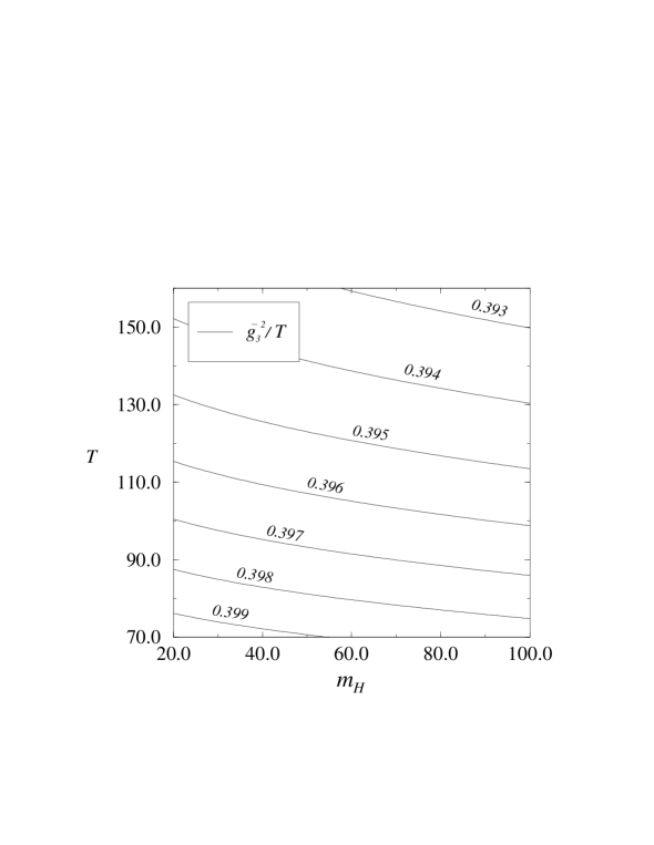
Figure 7: The scale $\bar{g}_{3}^{2}$ of the 3d SU(2)+Higgs theory divided by the temperature $T$, as a function of $m_{H}$ and $T$. The dependence of $\bar{g}_{3}^{2}/T$ on $m_{H}$ is caused by 1-loop corrections including the Higgs particle, and by the implicit dependence of $m_{W}$ on $m_{H}$ through Table 1. The dependence on temperature is caused by the logarithmic running in eq. (146).

Numerically, the properties of the 3d SU(2)$\times$U(1)+Higgs theory relevant for the EW phase transition can be presented as a function of the physical parameters through a few figures. First, put $m_{Z}\to m_{W}$ so that $g^{\prime}=0$. Then the final 3d theory has three parameters: the scale is given by $\bar{g}_{3}^{2}$, and the dynamics is given by the two dimensionless ratios $x=\bar{\lambda}_{3}/\bar{g}_{3}^{2}$, $y=\bar{m}_{3}^{2}(\bar{g}_{3}^{2})/\bar{g}_{3}^{4}$. The scale $\bar{g}_{3}^{2}$ is given as a function of $m_{H}$ and $T$ in Fig. 7, and the parameters $x$ and $y$ are given in Fig. 8. The phase diagram of the theory with the parameters $x$, $y$, together with the values of the latent heat, surface tension and correlation lengths in units of $\bar{g}_{3}^{2}$, have been studied with lattice MC simulations in [50].

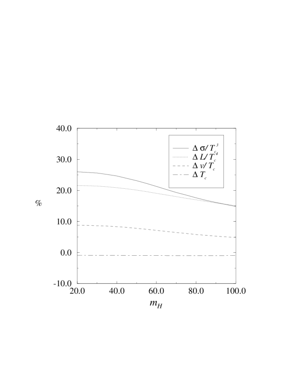
Figure 9: The percentual perturbative effect of the U(1)-subgroup on the critical temperature $T_{c}$, vacuum expectation value of the Higgs field $v(T_{c})/T_{c}$, latent heat $L/T_{c}^{4}$, and surface tension $\sigma/T_{c}^{3}$ as a function of the Higgs mass. For $v/T$, we have used the gauge-independent definition $v^{2}/T^{2}\equiv 2\langle\Phi_{3}^{\dagger}\Phi_{3}\rangle/T$. The surface tension is defined with the tree-level formula $\sigma=\int d\varphi\sqrt{2V(\varphi)}$. The effective potential $V(\varphi)$ here is the RG-improved 2-loop effective potential for the Higgs field [7] in the 3d SU(2)$\times$U(1)+Higgs theory (with the convention $g^{\prime 2}\sim g^{3}$).

Finally, one has to account for the effect of the U(1)-subgroup on the EW phase transition. Since there are no lattice simulations available for the 3d SU(2)$\times$U(1)+Higgs model, the best one can do is to estimate the effect of the U(1)-subgroup perturbatively. In Fig. 9, we display the percentual perturbative effect of the U(1)-subgroup on the critical temperature $T_{c}$, the vacuum expectation value of the Higgs field $v$, the latent heat $L$, and the surface tension $\sigma$ as a function of the physical Higgs mass. Using the non-perturbative values for the case $g^{\prime}=0$ from [50], one can then derive results for the full Standard Model.

5.4 The effect of higher-order operators

In Landau gauge in the Standard Model, the dominant 6-dimensional $\phi^{6}$-operators related to the integration over the superheavy scale are

$$O^{(6)}_{g^{2}} = \frac{3\zeta(3)}{16\,384\pi^{4}}\frac{g^{6}\phi^{6}}{T^{2}},$$ (195)

$$O^{(6)}_{g_{Y}^{2}} = -\frac{7\zeta(3)}{512\pi^{4}}\frac{g_{Y}^{6}\phi^{6}}{T^{2}}.$$ (196)

These follow from eq. (67) in Sec. 3. A complete list of the dominant fermionic contributions to the other 6-dimensional operators has been worked out in [41]. The dominant $\phi^{6}$-operator related to the integration over the heavy scale is

$$O^{(6)}_{\rm heavy}=\frac{3\sqrt{6/5}}{10\,240\pi}\frac{g^{3}\phi^{6}}{T^{2}}.$$ (197)

The 6-dimensional operators are neglected in the effective theories discussed in this paper, and their importance has to be estimated.

It is rather difficult to estimate the effect of the 6-dimensional operators comprehensively, apart from the powercounting estimate in Sec. 2. What can be done easily, though, is an evaluation of the shift caused by the $\phi^{6}$-operators in the vacuum expectation value of the Higgs field. A generic 6-dimensional operator $O^{(6)}=c\phi^{6}/T^{2}$ produces the term $\delta V=c\varphi^{6}/T^{2}$ to the effective potential $V(\varphi)$. Through

$$V^{\prime}(\varphi+\delta\varphi)+\delta V^{\prime}(\varphi)=0,$$ (198)

the relative shift induced is

$$\frac{\delta\varphi}{\varphi}=-\frac{\delta V^{\prime}}{\varphi V^{\prime\prime}}\approx-\frac{3c}{\lambda}\frac{\varphi^{2}}{T^{2}},$$ (199)

where it was assumed that $V^{\prime\prime}(\varphi)\sim 2\lambda\varphi^{2}$. For $m_{H}\sim m_{W}$ so that $\lambda\sim g^{2}/8$, the coefficients $3c/\lambda$ in the Standard Model following from eqs. (195), (196), (197) are

$$\biggl{(}\frac{3c}{\lambda}\biggr{)}_{g^{2}}\sim 10^{-5},\quad\biggl{(}\frac{3c}{\lambda}\biggr{)}_{g_{Y}^{2}}\sim-10^{-2},\quad\biggl{(}\frac{3c}{\lambda}\biggr{)}_{\rm heavy}\sim 10^{-3}.$$ (200)

The contributions from the top quark are seen to be dominant, and in the region where $\varphi/T\sim 1$, the effect of the corresponding 6-dimensional operator is of the order of one percent. Note that from the point of view of the 6-dimensional operators, the integration over the heavy scale is relatively better than the integration over the superheavy scale, although in terms of powers of coupling constants, the accuracy is worse. We conclude that the final 3d effective theory for the light fields should give results accurate within a few percent for all thermodynamic properties of the phase transition, like the latent heat, the surface tension, and the correlation lengths. For the critical temperature, the accuracy should be an order of magnitude better. In the pure SU(2)+Higgs theory without fermions, the accuracy of the theory with light and heavy fields should be better than 1% for all thermodynamic properties.

6 Discussion

The set of diagrams described and computed in Section 3 is sufficient to make a dimensional reduction of a large class of theories. In particular, it can be used for a construction of an effective 3d theory for different extensions of the Standard Model. Below we will argue that in many cases the effective theory appears to be just the SU(2)$\times$U(1)+Higgs model. We do not attempt to carry out the necessary computations here and discuss the general strategy only.

Let us take as an example the two Higgs doublet model. The integration over the superheavy modes gives a 3d SU(2)$\times$U(1) theory with two Higgs doublets, one Higgs triplet and one singlet (the last two are the zero components of the gauge fields). Construct now the 1-loop scalar mass matrix for the doublets and find the temperatures at which its eigenvalues are zero. Take the higher temperature; this is the temperature near which the phase transition takes place. Determine the mass of the other scalar at this temperature. Generally, it is of the order of $gT$, and therefore, is heavy. Integrate it out together with the heavy triplet and singlet – the result is the simple SU(2)$\times$U(1) model. In the case when both scalars are light near the critical temperature a more complicated model, containing two scalar doublets, should be studied. It is clear, however, that this case requires some fine tuning. The consideration of the phase transitions in the two Higgs doublet model on 1-loop level can be found in [42, 43].

The same strategy is applicable to the Minimal Supersymmetric Standard Model. If there is no breaking of colour and charge at high temperature (breaking is possible, in principle, since the theory contains squarks), then all degrees of freedom, excluding those belonging to the two Higgs doublet model, can be integrated out. We then return back to the case considered previously. The conclusion in this case is similar to the previous one, namely that the phase transition in MSSM can be described by a 3d SU(2)$\times$U(1) gauge-Higgs model, at least in a part of the parameter space. A 1-loop analysis of this theory was carried out in [44, 45, 46].

The procedure of dimensional reduction will give an infrared safe connection between the parameters of the underlying 4d theory and those of the 3d theory. The latter can then be studied by non-perturbative means, such as lattice Monte Carlo simulations [47, 48, 10, 49, 50].

Figure 1: The 2-loop graph (a) relevant for calculating the dimensionally reduced mass parameter in the “integration out”-procedure, and the additional graph (b) needed in the “matching” procedure. The thick lines are superheavy fields, and the thin dashed lines light fields.

Figure 2: The diagrams needed for the dimensional reduction of (a) the wave function $\phi$, and (b) the wave functions $A_{i}$ and $A_{0}$. Dashed line is a scalar propagator, wiggly line a vector propagator, double line a ghost propagator, and solid line a fermion propagator. The bare blob indicates the wave function counterterm.

Figure 3: The diagrams needed for calculating the 3d coupling constants $g_{3}^{2}$ and $h_{3}$.

Figure 4: The diagrams needed for calculating the 3d mass of the temporal components of the gauge fields.

Figure 5: The diagrams needed for calculating the quartic self-coupling of the temporal components of the gauge fields.

Figure 6: The diagrams needed for calculating the pole mass of (a) the Higgs particle, (b) the W boson and (c) the top quark. Curly line is the gluon propagator. For scalars, the counterterm indicated by the bare blob contains both the mass counterterm $\delta\nu^{2}$ and the counterterm from wave function renormalization. For vectors and fermions, the bare blob contains only the counterterm from wave function renormalization. The blobs with the short lines attached denote counterterms generated by the shift.

References

- [1] A.D. Linde, Phys. Lett. B 96 (1980) 289.
- [2] K. Farakos, K. Kajantie, K. Rummukainen and M. Shaposhnikov, Nucl. Phys. B 442 (1995) 317.
- [3] P. Ginsparg, Nucl. Phys. B 170 (1980) 388.
- [4] T. Appelquist and R. Pisarski, Phys. Rev. D 23 (1981) 2305.
- [5] S. Nadkarni, Phys. Rev. D 27 (1983) 917.
- [6] N.P. Landsman, Nucl. Phys. B 322 (1989) 498.
- [7] K. Farakos, K. Kajantie, K. Rummukainen and M. Shaposhnikov, Nucl. Phys. B 425 (1994) 67.
- [8] A. Jakovác, K. Kajantie and A. Patkós, Phys. Rev. D 49 (1994) 6810.
- [9] A. Jakovác and A. Patkós, Phys. Lett. B 334 (1994) 391.
- [10] F. Karsch, T. Neuhaus and A. Patkós, Nucl. Phys. B 441 (1995) 629.
- [11] J. Kripfganz, A. Laser and M.G. Schmidt, Phys. Lett. B 351 (1995) 266.
- [12] M. Laine, Phys. Lett. B 335 (1994) 173; Phys. Rev. D 51 (1995) 4525.
- [13] M. Laine, hep-lat/9504001, Nucl. Phys. B, to be published.
- [14] P. Lacock, D.E. Miller and T. Reisz, Nucl. Phys. B 369 (1992) 501.
- [15] L. Kärkkäinen, P. Lacock, B. Petersson and T. Reisz, Nucl. Phys. B 395 (1993) 733.
- [16] E. Braaten and A. Nieto, Phys. Rev. Lett. 73 (1994) 2402; E. Braaten, Phys. Rev. Lett. 74 (1995) 2164; E. Braaten and A. Nieto, Phys. Rev. Lett. 74 (1995) 3530; E. Braaten and A. Nieto, Phys. Rev. D 51 (1995) 6990.
- [17] S. Chapman, Phys. Rev. D 50 (1994) 5308.
- [18] S.-Z. Huang and M. Lissia, Nucl. Phys. B 438 (1995) 54.
- [19] P. Arnold and L. Yaffe, UW-PT-95-06 [hep-ph/9508280].
- [20] M. Dine, P. Huet, R.G. Leigh, A.D. Linde and D. Linde, Phys. Rev. D 46 (1992) 550.
- [21] M.E. Carrington, Phys. Rev. D 45 (1992) 2933.
- [22] W. Buchmüller, Z. Fodor, T. Helbig and D. Walliser, Ann. Phys. 234 (1994) 260.
- [23] P. Arnold and O. Espinosa, Phys. Rev. D 47 (1993) 3546; Phys. Rev. D 50 (1994) 6662 (Erratum).
- [24] Z. Fodor and A. Hebecker, Nucl. Phys. B 432 (1994) 127.
- [25] A. Jakovác, hep-ph/9502313.
- [26] U. Kerres, G. Mack and G. Palma, DESY-94-226 [hep-lat/9505008].
- [27] J.C. Collins, Renormalization (Cambridge University Press, 1984); G.P. Lepage, in From Actions to Answers, eds. T. DeGrand and D. Toussaint (World Scientific, Singapore, 1989).
- [28] P. Pascual and R. Tarrach, QCD: Renormalization for the Practitioner (Springer-Verlag, New York, 1984).
- [29] P. Arnold and C. Zhai, Phys. Rev. D 50 (1994) 7603; Phys. Rev. D 51 (1995) 1906.
- [30] A. Sirlin, Phys. Rev. D 22 (1980) 971.
- [31] A. Sirlin, Phys. Rev. D 29 (1984) 89.
- [32] M. Böhm, H. Spiesberger and W. Hollik, Fortschr. Phys. 34 (1986) 687.
- [33] W. Hollik, Fortschr. Phys. 38 (1990) 165.
- [34] D. Bardin et al., in CERN Report 95-03, Reports of the Working Group on Precision Calculations for the resonance, eds. D. Bardin, W. Hollik and G. Passarino (CERN, 1995).
- [35] A. Sirlin, Comm. Nucl. Part. Phys. 21 (1994) 287.
- [36] B.A. Kniehl, FERMILAB-PUB-95/247-T [hep-ph/9403386].
- [37] G. Montagna, O. Nicrosini, G. Passarino, F. Piccinini and R. Pittau, program TOPAZ0, [34]; Nucl. Phys. B 401 (1993) 3; Comput. Phys. Commun. 76 (1993) 328.
- [38] J.A. Casas, J.R. Espinosa, M. Quirós and A. Riotto, Nucl. Phys. B 436 (1995) 3; Nucl. Phys. B 439 (1995) 466 (Erratum).
- [39] Particle Data Group, Phys. Rev. D 50 (1994) 1173.
- [40] CDF Collaboration, Phys. Rev. Lett. 74 (1995) 2626; D0 Collaboration, Phys. Rev. Lett. 74 (1995) 2632.
- [41] G.D. Moore, private communication.
- [42] A.I. Bochkarev, S.V. Kuzmin and M.E. Shaposhnikov, Phys. Lett. B 244 (1990) 275; Phys. Rev. D 43 (1991) 369.
- [43] N. Turok and J. Zadrozny, Nucl. Phys. B 369 (1992) 729.
- [44] G.F. Giudice, Phys. Rev. D 45 (1992) 3177.
- [45] A. Brignole, J.R. Espinosa, M. Quirós and F. Zwirner, Phys. Lett. B 324 (1994) 181.
- [46] J.R. Espinosa, M. Quirós and F. Zwirner, Phys. Lett. B 307 (1993) 106.
- [47] K. Kajantie, K. Rummukainen and M. Shaposhnikov, Nucl. Phys. B 407 (1993) 356.
- [48] K. Farakos, K. Kajantie, K. Rummukainen and M. Shaposhnikov, Phys. Lett. B 336 (1994) 494.
- [49] E.M. Ilgenfritz, J. Kripfganz, H. Perlt and A. Schiller, HU-BERLIN-IEP-95/7 [hep-lat/9506023].
- [50] K. Farakos, K. Kajantie, M. Laine, K. Rummukainen and M. Shaposhnikov, in preparation.