Hyperon Decays in Chiral Perturbation Theory Revisited

Abstract

The discrepancies found between S-wave and P-wave fits for hyperon decays are reinvestigated using the heavy baryon chiral Lagrangian formalism. The agreement is found to improve through the inclusion of previously omitted diagrams. The S-waves are unaffected by this, but the P-wave predictions are modified. A correlated fit to the chiral parameters is performed and the results discussed.

August 1995

I Introduction

Chiral perturbation theory is an effective theory which obeys the symmetries of QCD and contains a number of parameters which must be determined experimentally. If the theory reflects nature, then the parameters should be universal. This can be tested through one-loop SU(3) breaking calculations for the decays of the octet and decuplet baryons. Uncalculable terms may yield corrections of up to 30 percent to these predictions, but if the variance in the comparison to experiment goes beyond this, the validity of the chiral expansion is questioned for that process, and the reliability of estimating unmeasured processes is open. The two-body weak $\Delta s=1$ decays of hyperons are a natural place to investigate the validity of chiral perturbation theory. The experimental observables have been well measured, and calculations including leading logarithmic corrections (which appear through one-loop SU(3) breaking diagrams) have been performed[1, 2]. A comparison of these results, however, showed that the parameters which fit the S-wave decays was inadequate for describing the P-wave decays. This caused concern about the legitimacy of the chiral Lagrangian expansion, at least for these processes[1, 3]. In this paper, previously omitted diagrams have been included in the calculation of P-wave amplitudes for nonleptonic hyperon decay. A correlated fit to the three weak parameters is performed and compared to previous results. The fit to the data improves markedly when one of the strong parameters, which is not well constrained at present, is also allowed to vary.

II The Chiral Lagrangian for Nonleptonic Decays.

Heavy Baryon Chiral Perturbation Theory (HBChPT), which is used to make predictions for hadronic processes at momentum transfers much less than one GeV, is introduced and well described in Ref.[4]. The weak interaction portion of the Lagrangian needed for $\Delta s=1$ hyperon decays, which transforms under ${\rm SU(3)_{L}}\otimes{\rm SU(3)_{R}}$ as an $(8_{L},1_{R})$, is outlined in Ref.[1, 2]. The Lagrangian

$${\cal L}={\cal L}_{strong}+{\cal L}_{weak}$$

contains the particles which are dynamic in the energy regime relevant for hyperon decay. This includes the lowest mass octet and decuplet of baryons, and the octet of pseudo-Goldstone bosons.

$${\cal L}_{strong} = i\ {\rm Tr}\ \bar{B}_{v}\ \left(v\cdot{\cal D}\right)B_{v}+2\ D\ {\rm Tr}\ \bar{B}_{v}\ S_{v}^{\mu}\ \{A_{\mu},B_{v}\}+2\ F\ {\rm Tr}\ \bar{B}_{v}\ S_{v}^{\mu}\ [A_{\mu},B_{v}]$$ (3)

$$-\ i\ \bar{T}_{v}^{\mu}\ (v\cdot{\cal D})\ T_{v\mu}+\Delta m\ \bar{T}_{v}^{\mu}\ T_{v\mu}+{\cal C}\ \left(\bar{T}_{v}^{\mu}\ A_{\mu}\ B_{v}+\bar{B}_{v}\ A_{\mu}\ T_{v}^{\mu}\right){\phantom{f^{2}\over 4}}$$

$$+\ 2\ {\cal H}\ \bar{T}_{v}^{\mu}\ S_{v\nu}\ A^{\nu}\ T_{v\mu}+{f^{2}\over 8}\ {\rm Tr}\ \partial_{\mu}\Sigma\partial^{\mu}\Sigma^{\dagger}+\mu\ {\rm Tr}\left(m_{q}\Sigma+m_{q}^{\dagger}\Sigma^{\dagger}\right)\ +\ \cdots\ \ \ \ ,$$

where $f\sim 93$ MeV is the meson decay constant, the light quark mass matrix $m_{q}={\rm diag}\{m_{u},m_{d},m_{s}\}$, and ${\cal D_{\mu}}=\partial_{\mu}+[V_{\mu},\;]$ is the covariant chiral derivative. The subscript $v$ on the baryon fields makes explicit that, in HBChPT, velocity is a good quantum number and labels the field for this portion of the Lagrangian. The actual full Lagrangian is a sum over all such velocities on terms like that above. The $B_{v}$ are the octet of baryons, and the $T_{v}^{\mu}$ are the decuplet of baryons (the $\mu$ index is the Lorentz superscript for this Rarita-Swinger field). The vector and axial vector chiral currents used are defined by

$$V_{\mu} = {1\over 2}(\xi\partial_{\mu}\xi^{\dagger}+\xi^{\dagger}\partial_{\mu}\xi)$$ (4)

$$A_{\mu} = {i\over 2}(\xi\partial_{\mu}\xi^{\dagger}-\xi^{\dagger}\partial_{\mu}\xi)\ \ \ .$$ (5)

Higher dimension operators, which contain more derivatives or insertions of the light quark mass matrix, are not needed in Eq. (3) to the order we are working. The octet of pseudo-Goldstone bosons, $M$, appears through

$$\Sigma=\xi^{2}={\rm exp}\left({2iM\over f}\right)\ \ \ .$$ (6)

The strong couplings constants $F,D,{\cal C}$, and ${\cal H}$ have been obtained by comparing one-loop computations of axial matrix elements between octet baryons to semileptonic baryon decay measurements[4]. The constants ${\cal C}$ and ${\cal H}$ are further constrained through the one-loop computation of the strong decays of decuplet baryons [5]. This yields,

$$D=0.6\pm 0.1 F=0.4\pm 0.1\ \$$ (7)

$$1.1<|{\cal C}|<1.8 -2.8<{\cal H}<-1.6\ \ \ \ ,$$ (8)

Note that the sign of ${\cal C}$ remains a convention. The errors do not include theoretical errors.

Assuming octet dominance (the $\Delta I={1\over 2}$ rule), the $\Delta s=1$ weak Lagrangian is

$${\cal L}_{weak} = G_{F}\ m_{\pi}^{2}\ \sqrt{2}f_{\pi}\ h_{D}\ {\rm Tr}\ {\overline{B}}_{v}\ \{\xi^{\dagger}h\xi\,,B_{v}\}\;+\;G_{F}\ m_{\pi}^{2}\ \sqrt{2}f_{\pi}\ h_{F}\ {\rm Tr}\ {\overline{B}}_{v}\ {[\xi^{\dagger}h\xi\,,B_{v}]}\;$$ (10)

$$+G_{F}\ m_{\pi}^{2}\ \sqrt{2}f_{\pi}\ h_{C}\ {\overline{T}}^{\mu}_{v}\ (\xi^{\dagger}h\xi)\ T_{v\mu}\;+\;G_{F}\ m_{\pi}^{2}\ h_{\pi}\ {f_{\pi}^{2}\over 4}\ {\rm Tr}\left(h\,\partial_{\mu}\Sigma\partial^{\mu}\Sigma^{\dagger}\right)\ +\ \cdots\ ,$$

where

$$h=\left(\matrix{0&0&0\cr 0&0&1\cr 0&0&0}\right)\ \ \ ,$$ (11)

picks out just the $\Delta s=1$ piece needed for hyperon decays. The constants $f_{\pi}$, $h_{D},h_{F},h_{\pi}$ and $h_{C}$ are then fit to reproduce experimental data. Predictive power is obtained because there are many more observables than parameters. The pion decay constant $f_{\pi}\sim 93$ MeV. Factors of $G_{F}m_{\pi}^{2}\sqrt{2}f_{\pi}$ are inserted in Eq. (10) so that the constants $h_{D}$, $h_{F}$, and $h_{C}$ are dimensionless. Nonleptonic kaon decays suggest that the weak meson coupling $h_{\pi}=1.4$.

III Hyperon Decay Amplitudes

In this section, the formulae for the S-wave and P-wave amplitudes for $\Delta S=1$ nonleptonic hyperon decay are discussed. The S-wave amplitudes were calculated previously[2]. The portion of the P-wave amplitudes coming from the diagrams in Figure 1 were also calculated in [2]. The pieces which are new and the subject of this work affect the P-wave amplitudes and arise from the diagrams in Figure 2.

The total amplitude for a decay of an initial octet baryon to a final octet baryon, $B_{i}\rightarrow B_{f}\pi$ is given by

$${\cal A}=i\ G_{F}\ m_{\pi}^{2}\ \sqrt{2}\ f_{\pi}\ \overline{u}_{B_{f}}\ \left[{\cal A}^{(S)}+2k\cdot S_{v}{\cal A}^{(P)}\right]u_{B_{i}}\ \ \ ,$$ (12)

where $k$ is the outgoing momentum of the pion and $S_{v}$ is the spin operator for the baryons. The amplitudes ${\cal A}^{(S)}$ and ${\cal A}^{(P)}$ are the S-wave and P-wave amplitudes. Of all physically possible decays within the octet of baryons, only four are independent after isospin symmetry has been imposed. In keeping with Refs. [1, 2], we will continue to choose those four to be $\Sigma^{+}\rightarrow n\pi^{+}$, $\Sigma^{-}\rightarrow n\pi^{-}$, $\Lambda\rightarrow p\pi^{-}$, and $\Xi^{-}\rightarrow\Lambda\pi^{-}$. The results will be given using the following definitions of ${\cal A}^{(S)}$ or ${\cal A}^{(P)}$:

$${\cal A}^{S,P}_{if}=\alpha^{S,P}_{if}+\left(\beta^{S,P}_{if}-\lambda^{S,P}_{if}\ \alpha^{S,P}_{if}\right){m_{K}^{2}\over 16\pi^{2}f_{K}^{2}}\log\left({m_{K}^{2}\over\Lambda_{\chi}^{2}}\right)\ \ \ ,$$ (13)

where

$$\beta^{(P)}_{if}=\beta^{(P1)}_{if}+\beta^{(P2)}_{if}\ \ .$$ (14)

The kaon decay parameter and mass are $f_{K}$ and $m_{K}$, respectively, and the chiral symmetry breaking scale, $\Lambda_{\chi}\sim 1$ GeV.

The $\alpha^{(S)}_{if}$, $\beta^{(S)}_{if}$ (including both octet and decuplet intermediate states, denoted $\overline{\beta}^{(S)}_{if}$ in Ref.[2]), and $\lambda^{(S)}_{if}$ terms can be found in Ref.[2]. Despite apparent differences in amplitude definitions, these can be taken straight across because of the units used. The values finally obtained will be different simply because the fit to parameters will include the changes in the P-wave amplitudes.

Similarly, the $\alpha^{(P)}_{if}$ and $\lambda^{(P)}_{if}$ are unaffected by the inclusion of the graphs in Figure 2. The $\overline{\beta}^{(P)}_{if}$ in Ref.[2] will now be called $\beta^{(P1)}_{if}$ and the new graphs will give $\beta^{(P2)}_{if}$. The diagrams in Fig. 2 yield

$$\beta^{(P2)}_{\Sigma^{+}n} = {D\over 3}{h_{D}+3h_{F}\over m_{\Lambda}-m_{N}}\ \lambda_{\Lambda}+F\ {h_{F}-h_{D}\over m_{\Sigma}-m_{N}}\ \lambda_{\Sigma}-{(F+D)(h_{F}-h_{D})\over m_{\Sigma}-m_{N}}\ \lambda_{N}$$ (15)

$$\beta^{(P2)}_{\Sigma^{-}n} = {D\over 3}\ {h_{D}+3h_{F}\over m_{\Lambda}-m_{N}}\ \lambda_{\Lambda}-F\ {h_{F}-h_{D}\over m_{\Sigma}-m_{N}}\ \lambda_{\Sigma}$$ (16)

$$\beta^{(P2)}_{\Lambda p} = {2D\over\sqrt{6}}\ {h_{F}-h_{D}\over m_{\Sigma}-m_{N}}\ \lambda_{\Sigma}-{F+D\over\sqrt{6}}\ {3h_{F}+h_{D}\over m_{\Lambda}-m_{N}}\ \lambda_{N}$$ (17)

$$\beta^{(P2)}_{\Xi\Lambda} = -\ {D-F\over\sqrt{6}}\ {3h_{F}-h_{D}\over m_{\Xi}-m_{\Lambda}}\ \lambda_{\Xi}+{2D\over\sqrt{6}}\ {h_{F}+h_{D}\over m_{\Xi}-m_{\Sigma}}\ \lambda_{\Sigma}\ \ \ ,$$ (18)

with

$$\lambda_{N} = {17\over 6}D^{2}-5DF+{15\over 2}F^{2}+{1\over 2}{\cal C}^{2}$$ (19)

$$\lambda_{\Lambda} = {7\over 3}D^{2}+9F^{2}+{\cal C}^{2}$$ (20)

$$\lambda_{\Sigma} = {13\over 3}D^{2}+3F^{2}+{7\over 3}{\cal C}^{2}$$ (21)

$$\lambda_{\Xi} = {17\over 6}D^{2}+5FD+{15\over 2}F^{2}+{13\over 6}{\cal C}^{2}\ \ .$$ (22)

IV Discussion

The amplitudes obtained from including the diagrams in Fig. 2 are shown in Tables 1 and 2. The experimental measurements, including errors, are shown in the first column. The second column contains the tree level SU(3) predictions, where the chiral parameters used are the ones extracted from tree-level fits. The third column shows the results of Ref. [2].

The fourth column contains the chiral one-loop predictions using weak parameters obtained by fitting only to the S-wave experimental values. To most closely match the analysis of Ref. [2], the strong interaction couplings are chosen to be F=0.4, D=0.61, $|{\cal C}|=1.6$, and ${\cal H}=-1.9$. Letting the weak parameters $h_{D}$, $h_{F}$, and $h_{C}$ vary, a fit to the S-wave decays yields [6]

$$h_{D}=-0.32\pm 0.01,\hskip 28.45274pth_{F}=0.98\pm 0.03,\hskip 28.45274pth_{C}=-1.37\pm 0.27\ \ .$$ (23)

The errors shown are only those which arise from the experimental variances. The parameter $h_{C}$ is not well determined and large variations in its value do not appreciably change the predicted amplitudes. The S-wave predictions are essentially unchanged using the parameters above, and the loop corrected chiral predictions are in excellent agreement with experiment, as demonstrated in Ref. [2]. The situation for the P-wave predictions is improved for $\Sigma^{+}\rightarrow n\pi^{+}$, where the agreement is within the allowed 30 percent variation for chiral predictions. For the decays $\Sigma\rightarrow n\pi^{-}$ and $\Lambda\rightarrow p\pi^{-}$, the additional graphs bring the prediction back to tree level values, while the $\Xi\rightarrow\Lambda\pi^{-}$ decay remains essentially unchanged.

The fifth column in Tables 1 and 2 contains the results from using both S-wave and P-wave amplitudes to fit the weak chiral parameters. The tree level $\Omega$ decays for which there are experimental results are used as well. Expressions for these are in Ref. [2]. The strong decays of the decuplet favor midpoint values for $|{\cal C}|$ and ${\cal H}$ of 1.2 and –2.2, respectively [5]. A fit to $h_{D}$, $h_{F}$, and $h_{C}$ in this scenario yields

$$h_{D}=-0.38\pm 0.01,\hskip 28.45274pth_{F}=0.92\pm 0.01,\hskip 28.45274pth_{C}=0.74\pm 0.18\ \ .$$ (24)

The S-waves are still within 30 percent, but the P-waves get worse. The nonleptonic hyperon decays clearly favor a larger value for $|{\cal C}|$ than do the strong decuplet decays. The dependence on ${\cal H}$ is not as sensitive.

Using the eight independent nonleptonic hyperon decays, along with the $\Omega$ decays, and ${\cal H}=-2.2$, the parameters ${\cal C}$, $h_{D}$, $h_{F}$, and $h_{C}$ are allowed to vary. The best fit is obtained when

$$|{\cal C}|=1.76\pm 0.01 h_{D}=-0.42\pm 0.01,$$ (25)

$$h_{F}=0.76\pm 0.01 h_{C}=0.26\pm 0.10$$ (26)

The matrix of correlation coefficients for this fit, given in the order ($h_{C}$, $h_{D}$, $h_{F}$, ${\cal C}$) is

$$\left(\begin{array}[]{rrrr}1.000&-0.914&-0.974&0.149\\ -0.914&1.000&0.919&-0.024\\ -0.974&0.919&1.000&-0.009\\ 0.149&-0.024&-0.009&1.000\\ \end{array}\right)$$ (31)

The S-wave and P-wave amplitude predictions using these parameters are given in the final column of each Table. The S-waves remain well described, and all but the $\Lambda\rightarrow p\pi^{-}$ P-wave modes do as well as the S-waves. This later decay amplitude becomes positive for parameter values still within ranges allowed by other observables, but the agreement remains poor. Still, the additional diagrams have improved the situation to the point where the chiral expansion appears to be on more solid footing with respect to the P-wave decays. As Jenkins points out in Ref. [2], the large corrections which the loop diagrams give to the tree-level results need not be taken as evidence that the chiral expansion is ill-behaved if it is the leading order terms which are anomalously small rather than the loop effects which are unnaturally large.

	S-waves
decay	exp	tree	theory[2]	theory (S)	theory ($\Delta$)	theory
$\hskip 5.69046pt\Sigma^{+}\rightarrow n\pi^{+}$	0.06 $\pm$ 0.01	0.00	–0.09	–0.09	0.00	–0.13
$\hskip 5.69046pt\Sigma^{-}\rightarrow n\pi^{-}$	1.88$\pm$0.01	1.21	1.90	1.88	1.74	1.90
$\hskip 5.69046pt\Lambda\rightarrow p\pi^{-}$	1.42$\pm$0.01	0.91	1.44	1.42	1.44	1.28
$\hskip 5.69046pt\Xi^{-}\rightarrow\Lambda\pi^{-}$	–1.98$\pm$0.01	–1.19	–2.04	–1.98	–1.91	–2.02

Table 1. The S-wave $\Delta s=1$ hyperon amplitudes. The first column is the experimental result and the next is the tree level prediction of chiral perturbation theory [1, 2]. The third column contains the loop corrected results of Ref.[2]. The “theory (S)” column gives the fit using S-wave predictions only, with the Ref. [2] values $|{\cal C}|$ = 1.6 and ${\cal H}$ = –1.9. The “theory ($\Delta$)” column fits both S-wave and P-wave expressions, but uses $|{\cal C}|$=1.2 and ${\cal H}$ = –2.2 taken from the strong decuplet decays. The last column uses the parameters which were obtained from a best fit including both S-waves and P-waves, ${\cal H}$ = –2.2, and ${\cal C}$ fit, including the diagrams of Fig. 2.

	P-waves
decay	exp	tree	theory[2]	theory (S)	theory ($\Delta$)	theory
$\hskip 14.22636pt\Sigma^{+}\rightarrow n\pi^{+}$	1.81$\pm$0.01	–0.06	0.82	1.54	1.10	1.83
$\hskip 5.69046pt\Sigma^{-}\rightarrow n\pi^{-}$	–0.06$\pm$0.01	0.13	0.34	0.16	0.34	–0.04
$\hskip 5.69046pt\Lambda\rightarrow p\pi^{-}$	0.52$\pm$0.02	–0.28	–0.52	–0.27	–0.51	–0.11
$\hskip 5.69046pt\Xi^{-}\rightarrow\Lambda\pi^{-}$	0.48$\pm$0.02	0.11	0.35	0.34	0.67	0.48

Table 2. The P-wave $\Delta s=1$ hyperon amplitudes. The first column is the experimental result and the next is the tree level prediction of chiral perturbation theory [1, 2]. The third column contains the loop corrected results of Ref.[2]. The column labelled “theory (S)” uses the parameters obtained from fitting to the S-wave expressions only, with $|{\cal C}|$ = 1.6 and ${\cal H}$ = –1.9, and includes the P-wave diagrams of Fig. 2. The “theory ($\Delta$)” column fits both S-wave and P-wave decays, but uses $|{\cal C}|$=1.2 and ${\cal H}$ = –2.2 taken from strong decuplet decays. The last column is the result of parameters extracted from a best fit of both S-wave and P-wave expressions, with ${\cal H}$ = –2.2, and ${\cal C}$ fit, including the diagrams of Fig. 2.

V Acknowledgements

I would like to thank the Institute for Nuclear Theory at the University of Washington, where much of this work was completed, for their kind hospitality. I gratefully acknowledge advice from Martin Savage and Ted Allen. I thank Martin for many discussions and his always interesting observations and suggestions, and Ted for invaluable assistance with computers, codes, and error analysis. This work is supported in part by the US Dept. of Energy under grant number DE-FG05-90ER40592.

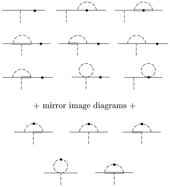
FIG. 1.: Feynman diagrams for P-wave $\Delta s=1$ hyperon decay calculated in Ref. [2]. The wavefunction renormalization graphs are not shown. The dashed lines are mesons, and the solid lines are octet baryons. The unmarked vertex is a strong interaction and the black dots are weak vertices.

FIG. 2.: Feynman diagrams for P-wave $\Delta s=1$ hyperon decay included, in addition to the ones in Figure 1, in the present calculation. The dashed lines are mesons, and the solid lines are octet baryons. The unmarked vertex is a strong interaction and the black dots are weak vertices.

REFERENCES

• [1] J. Bijnens, H. Sonoda, and M.B. Wise, Nucl. Phys. B261 (1985) 185.
• [2] E. Jenkins, Nucl. Phys. B375 (1992) 561.
• [3] C. Carone and H. Georgi, Nucl. Phys. B375 (1992) 243.
• [4] E. Jenkins and A. Manohar, Phys. Lett. B255 (1991) 558; B259 (1991) 353.
• [5] M.N. Butler, M.J. Savage and R.P. Springer, Nuc. Phys. B399 (1993) 69.
• [6] All fits here were performed using MINUIT, the Function Minimization and Error Analysis program written by F. James, CERN Program Library entry D506, Geneva, 1994.
Refer to caption