THE $\xi(2220)$ REVISITED:
STRONG DECAYS OF THE $1^{3}F_{2}$ and $1^{3}F_{4}$ $s\bar{s}$ MESONS

Abstract

We calculated the decay widths of the $1^{3}F_{2}$ and $1^{3}F_{4}$ $s\bar{s}$ mesons and compared them to the measured properties of the $\xi(2220)$ (now known as the $f_{4}(2220)$). Including previously neglected decay modes we found that the width of the ${}^{3}F_{2}$ state $s\bar{s}$ meson is much larger than previously believed making this explanation unlikely. On the other hand the predicted width of the ${}^{3}F_{4}$ state, although broader than the observed width, is consistent within the uncertainties of the model. This interpretation predicts large partial widths to $KK^{*}(892)$ and $K^{*}(892)K^{*}(892)$ final states which should be looked for. A second possibility that would account for the different properties of the $\xi(2220)$ seen in different experiments is that two hadronic states exist at this mass. The first would be a broader ${}^{3}F_{4}$ $s\bar{s}$ state which is seen in hadron beam experiments while the second would be a narrow state with high glue content seen in the gluon rich $J/\psi$ radiative decay. Further experimental results are needed to sort this out.

I INTRODUCTION

It is roughly a decade since the $\xi(2220)$, now known as the $f_{4}(2220)$, was discovered by the MARK III collaboration in $J/\psi$ radiative decays to $K^{+}K^{-}$ and $K_{S}K_{S}$ final states [1]. Its most interesting property, which attracted considerable attention, was its narrow width of roughly 30 MeV. Because the width was inconsistent with expectations for a conventional $q\bar{q}$ meson with such a large mass, the $\xi$’s discovery led to speculation that it might be a Higgs boson [2], a bound state of coloured scalars [3], a four quark state [4, 5], a $\Lambda\bar{\Lambda}$ bound state [6], a hybrid [7], or a glueball [8]. Despite the prevailing wisdom, the authors of Ref. [9, 5] argued that the properties of the $\xi(2220)$ could be consistent with those of a conventional meson: the L=3 $s\bar{s}$ meson with $J^{PC}=2^{++}$ or $J^{PC}=4^{++}$.

In the original analysis of L=3 $s\bar{s}$ properties it was shown that of the $q\bar{q}$ states with the appropriate $J^{PC}$ quantum numbers only the ${}^{3}F_{2}$ and ${}^{3}F_{4}$ $s\bar{s}$ states of the first L=3 multiplet have masses consistent with the $\xi(2220)$ [9]. According to this analysis these two states were exceptional in that they have a limited number of available decay modes which are all relatively weak. However, the analysis was not exhaustive in that it did not calculate the decay widths to all possible final states. In particular it made the assumption, which we will see to be incorrect, that the decays to an $L=1$ meson and a $K$ or $\eta$ were small on the basis of phase space arguments alone.

To further complicate the discussion, more recent experiments have observed a hadronic state decaying to $K\bar{K}$ in different reactions and with different properties. The various experimental results relevant to the $\xi(2220)$ are summarized in Table I. The most recent measurement of the $\xi(2220)$ properties by the BES collaboration [11] indicates that its decays are approximately flavour symmetric giving support to the glueball interpretation. At the same time, although the narrow $\xi(2220)$ was not seen in $J/\psi$ radiative decays by the DM2 experiment despite the fact that DM2 has slightly higher statistics, DM2 did observe a broader state decaying into $K\bar{K}$ [10]. If all the experiments are taken at face value the overall picture is confused and contradictory.

In this paper we re-examine the nature of the $\xi(2220)/f_{4}(2220)$ meson and calculate the partial widths of the ${}^{3}F_{2}$ and ${}^{3}F_{4}$ $s\bar{s}$ states to all OZI-allowed 2-body final states allowed by phase space. To give a measure of the reliability of our analysis we calculate the widths using both the ${}^{3}P_{0}$ decay model (often referred to as the quark-pair creation decay model) [15, 16] and the flux-tube breaking decay model [17]. As an additional consistency check we calculated several partial widths using the pseudoscalar decay model [18]. Our goal is to shed some light on the nature of the $\xi(2220)$ by comparing the quark model predictions for the hadronic widths to the various experimental results.

The outline of the paper is as follows. In section II we briefly outline the models of hadron decays and the fitting of the parameters of the models. We relegate the details to the appendices. In section III we present the results of our calculations for the $L=3$ mesons and discuss our results. In the final section we attempt to make sense of the various contradictory experimental results and put forward our interpretation along with some suggested measurements which may clear up the situation.

II MODELS OF MESON PROPERTIES AND DECAYS

The quark model has proven to be a useful tool to describe the properties of hadrons. The quark model has successfully described weak, electromagnetic, and strong couplings . In some cases we will use simplified meson wavefunctions which have been used elsewhere to describe hadronic decays [17] while in other cases we will use more complicated wavefunctions from a relativized quark model which includes one-gluon exchange and a linear confining potential [18]. The strong decay analysis was performed using the QCD based flux-tube breaking model [17]. It has the attractive feature of describing decay rates to all possible final states in terms of just one fitted parameter. We also include results for the ${}^{3}P_{0}$ model, often referred to as the quark-pair creation model [15, 16], which is a limiting case of the flux-tube breaking model and which greatly simplifies the calculations and gives similar results. As a final check we calculated some partial widths using the pseudoscalar emission model [18] and confirmed that it also gave results similar to those of the flux-tube breaking model.

A Decays by the ${}^{3}P_{0}$ Model

The ${}^{3}P_{0}$ model [15, 16] is applicable to OZI-allowed strong decays of a meson into two other mesons, as well as the two-body strong decays of baryons and other hadrons. Meson decay occurs when a quark-antiquark pair is produced from the vacuum in a state suitable for quark rearrangement to occur, as in Fig. 1. The created pair will have the quantum numbers of the vacuum, ${}^{3}P_{0}$. There is one undetermined parameter $\gamma$ in the model - it represents the probability that a quark-antiquark pair will be created from the vacuum. The rest of the model is just the description of the overlap of the initial meson (A) and the created pair with the two final mesons (B,C), to calculate the probability that rearrangement (and hence decay) will occur. A brief description of the model is included in Appendix A, and the techniques by which the calculations were performed are discussed in Appendices C and D.

B Decays by the Flux-Tube Breaking Model

In the flux-tube picture a meson consists of a quark and antiquark connected by a tube of chromoelectric flux, which is treated as a vibrating string. For mesons the string is in its vibrational ground state. Vibrational excitations of the string would correspond to a type of meson hybrid, particles whose existence have not yet been confirmed.

The flux-tube breaking decay model [17] is similar to the ${}^{3}P_{0}$ model, but extends it by considering the actual dynamics of the flux-tubes. This is done by including a factor representing the overlap of the flux-tube of the initial meson with those of the two outgoing mesons. A brief review of the model is given in Appendix B, and the techniques by which the calculations were performed are discussed in Appendices C and D.

C Fitting the Parameters of the Decay Models

The point of these calculations is to obtain a reliable estimate of the ${}^{3}F_{2}$ and ${}^{3}F_{4}$ $s\bar{s}$ meson decay widths. To do so we considered several variations of the flux-tube breaking model. By seeing how much the results vary under the various assumptions we can estimate the reliability of the predictions.

The first variation lies with the normalization of the mock meson wavefunctions and the phase space used to calculate the decay widths [19]. In the Appendices we have normalized the mock meson wavefunctions relativistically to $2E$ and used relativistic phase space, which leads to a factor of $E_{B}E_{C}/M_{A}$ in the final expression for the width in the centre of mass frame. We will refer to this as relativistic phase space/normalization (RPSN). However, there are arguments [20] that heavy quark effective theory fixes the assumptions in the mock meson prescription and suggests that the energy factor be replaced by $\widetilde{M}_{B}\widetilde{M}_{C}/\widetilde{M}_{A}$, where the $\widetilde{M}_{i}$ are the calculated masses of the meson $i$ in a spin-independent quark-antiquark potential [17]. (In other words $\widetilde{M}_{i}$ is given by the hyperfine averaged mass that is equal to the centre of gravity of the triplet and singlet masses of a multiplet of given $L$.) We will refer to this as the Kokoski-Isgur phase space/normalization (KIPSN).

The second variation in our results is the choice of wavefunctions. We calculate decay widths for two cases. In the first we use simple harmonic oscillator (SHO) wavefunctions with a common oscillator parameter for all mesons. In the second case we use the wavefunctions, calculated in a relativized quark model, of Ref. [18] which we will label RQM. In all we looked at six cases: the ${}^{3}P_{0}$ model using the SHO wavefunctions, the flux-tube breaking model again using the SHO wavefunctions, and the flux-tube breaking model using the RQM wavefunctions of Ref. [18]; in all three cases we used both choices of phase space/normalization.

Some comments about the details of the calculations are in order. For the SHO wavefunctions, we took for the oscillator parameter $\beta=400$ MeV which is the value used by Kokoski and Isgur [17]. However, different quark models find different values of $\beta$ so that there is the question of the sensitivity of our results to $\beta$. We will address this issue below. We used quark masses in the ratio $m_{u}:m_{d}:m_{s}=3:3:5$ — this differs from the calculations of Ref. [17], which ignored the strange-quark mass difference. In the RQM wavefunctions these parameters are already set — the values of $\beta$ were found individually for each meson, and the quark masses were fitted: $m_{u}=220$ MeV, $m_{d}=220$ MeV, and $m_{s}=419$ MeV. We have treated all mesons as narrow resonances, and have ignored mass differences between members of the same isospin multiplet . Masses were taken from the Review of Particle Properties 1994 [21] if the state was included in their Meson Summary Table . If it was not, then the masses predicted in Ref. [18] were used. (This includes the masses of the $1^{3}F_{2}$ and $1^{3}F_{4}$ $s\bar{s}$ mesons: 2240 MeV and 2200 MeV respectively.) Meson flavour wavefunctions were also taken from Ref. [18] - for the isoscalars we assumed ideal mixing ($\phi_{\rm nonstrange}=\frac{1}{\sqrt{2}}(u\bar{u}+d\bar{d})$, $\phi_{\rm strange}=s\bar{s}$), except for the radial ground state pseudoscalars, where we assumed perfect mixing ($\phi_{\eta}=\frac{1}{\sqrt{2}}(\phi_{\rm nonstrange}-\phi_{\rm strange})$, $\phi_{\eta^{\prime}}=\frac{1}{\sqrt{2}}(\phi_{\rm nonstrange}+\phi_{\rm strange})$).

We fitted $\gamma$, the one undetermined parameter of the model, in a global least squares fit of 28 of the best known meson decays. (We minimized the quantity defined by $\chi^{2}=\sum_{i}(\Gamma^{model}_{i}-\Gamma^{exp}_{i})^{2}/\sigma_{\Gamma_{i}}^{2}$ where $\sigma_{\Gamma_{i}}$ is the experimental error .) The experimental values for these decays and the fitted values for the six cases are listed in Table II. To give a more descriptive picture of the results we plotted in Fig. 2, on a logarithmic scale, the ratio of the fitted values to the experimental values. From Table II one can see that the results for the ${}^{3}P_{0}$ and flux-tube breaking models for the SHO wavefunctions are very similar. We therefore only plotted the ${}^{3}P_{0}$ model results using the SHO wavefunctions and the flux-tube breaking model results for the RQM wavefunctions. A reference line is drawn in each case for $\Gamma^{model}/\Gamma^{exp}=1$ to guide the eye. Since all the partial widths are proportional to $\gamma^{2}$, using a different fit strategy rescales $\gamma$. This is equivalent to simply shifting all points on the plot simultaneously making it easy to visualize any change in agreement for specific decays.

The KIPSN gives a better overall fit to the data. Even so, certain decays, $K_{3}^{*}(1780)\to K\rho$ and $f_{4}(2050)\to\omega\omega$ for example, are fit much better using the RPSN. For both the RPSN and KIPSN one can see in Fig. 2 that a significant number of the decays differ from the experimental values by factors of two or more. Decays with two pseudoscalars in the final state tend to do better with the KIPSN but the KIPSN generally underestimates decays of high L mesons with vector mesons in the final states. On the other hand the RPSN tends to overestimate decays with two pseudoscalars in the final states. Similar observations can be made for the flux-tube breaking model using the RQM wavefunctions. Having said all this we stress that these are only general observations and exceptions can be found to any of them in Table II. One must therefore be very careful not to take the predictions at face value but should try if possible to compare the predicted decay to a similar one that is experimentally well known.

Finally, we consider the sensitivity of our results to $\beta$. In addition to the fits discussed above, we performed simultaneous fits of both $\gamma$ and $\beta$ to the 28 decay widths for both the RPSN and the KIPSN. The resulting values of $\gamma$ and $\beta$ are 13.4 and 481 MeV respectively for RPSN and 5.60 and 371 MeV respectively for KIPSN. In both cases the overall fits improved slightly, with some widths in better agreement and some in worse agreement with experiment when compared to the fits for $\beta=400$ MeV. However, the fitted widths of the most relevant ${}^{3}F_{4}$ decays improve slightly for RPSN but show mixed results for KIPSN. We also redid our fits of $\gamma$ to the decay widths for $\beta=350$ GeV and $\beta=450$ GeV. For $\beta=350$ MeV the overall fit improves slightly for KIPSN although the predicted $f_{4}(2050)$ decay widths are a little worse and the $K_{4}(2045)$ widths are a little better. For RPSN the overall fit is a little worse as are the ${}^{3}F_{4}$ decays. For $\beta=450$ MeV the overall fit with KIPSN becomes a little worse as does the fitted ${}^{3}F_{4}$ widths while for RPSN the overall fit and fitted ${}^{3}F_{4}$ widths become a little better. We conclude that while there is some sensitivity to $\beta$, the results for modest changes in $\beta$ (including the $\beta$ we obtain by fitting $\gamma$ and $\beta$ simultaneously) are consistent with those for $\beta=400$ MeV within the overall uncertainty we assign to our results. It should be stressed that it is not sufficient to simply change $\beta$ but that a new value of $\gamma$ must be fitted to the experimental widths included in our fit.

III RESULTS FOR ${}^{3}F_{2}$ and ${}^{3}F_{4}$ $s\bar{s}$ MESON DECAYS

Using the $\gamma$’s obtained from our fit we calculated all kinematically allowed partial widths for the ${}^{3}F_{2}$ and ${}^{3}F_{4}$ $s\bar{s}$ meson decays. The results are given in Tables III and IV.

For the ${}^{3}F_{4}$ state the main decay modes are:

$$f_{4}^{\prime}\to K^{*}(892)K^{*}(892),\;K\bar{K},\;KK^{*}(892),\;\phi\phi,\;KK_{2}^{*}(1430),\;KK_{1}(1400),\;\eta\eta,\;\eta\eta^{\prime}$$ (1)

For the KIPSN and the SHO wavefunctions the total width is 132 MeV with the ${}^{3}P_{0}$ model. For this set of assumptions the $K\bar{K}$, $\eta\eta$, and $\eta\eta^{\prime}$ modes are probably reasonably good estimates. However, the decay widths to $KK^{*}(892)$ and $K^{*}(892)K^{*}(892)$ are likely to be larger than the predictions. On this basis it does not seem likely to us that the $f_{4}^{\prime}$ width is less than the predicted total width by a factor of two or more, i.e. we do not expect it to be less than about 70 MeV. If anything, we would expect it to be larger than the predicted width, i.e. $>140$ MeV.

For the ${}^{3}F_{2}$ state we obtain results similar to the ${}^{3}F_{4}$ state for the $K\bar{K}$, $KK^{*}(892)$, and $K^{*}(892)K^{*}(892)$ modes. However, the ${}^{3}F_{2}$ also has large partial widths to $KK_{1}(1270)$, $K^{*}(892)K_{1}(1270)$, $KK_{2}^{*}(1430)$ and $\eta f_{1}(1510)$. In fact, $KK_{1}(1270)$ is the dominant decay mode. It is large in all variations of the calculation we give in Table IV. The most closely related decay in our fit is the decay $\pi_{2}(1670)\to f_{2}(1270)\pi$ which is relatively large and is well reproduced by the KI normalization and SHO wavefunction case. The total width for this case is $\sim 400$ MeV . Even if this width is overestimated by a factor of two, it would still be too large to identify with the $\xi(2220)$.

Although this result appears surprising it has a straightforward explanation. Examining Table IV, the lowest angular momentum final states in $f_{2}^{\prime}$ decay are P-waves. All of these decays are relatively broad but the $f_{2}^{\prime}\to K_{1}(1270)K$ is the P-wave decay with the largest available phase space. In fact, one could almost order the P-wave decays using phase space alone. The analogous decay of the $f_{4}^{\prime}$ is in an F-wave and therefore is subject to a larger angular momentum barrier. The lowest angular momentum partial wave for $f_{4}^{\prime}$ decays is a D-wave which although it has the largest partial width of all $f_{4}^{\prime}$ decays is still smaller than the P-wave $f_{2}^{\prime}$ decay.

As another measure of the reliability of these predictions we calculated the widths of the $K_{4}^{*}(2045)$ and $f_{4}(2050)$ mesons (the ${}^{3}F_{4}$ $K$-like and non-strange isovector mesons, respectively). The results for all significant kinematically allowed final states are given for the ${}^{3}P_{0}$ model using SHO wavefunctions in Tables V and VI respectively. The results are consistent with the general fit results given in Table II and Fig. 2. In general, the widths calculated using RPSN tend to be larger and those calculated using the KIPSN tend to be smaller. More specifically, decays to two pseudoscalar mesons using RPSN are generally overestimated while the results calculated using KIPSN are in reasonable agreement with experiment. There is no pattern for the decays to two vector final states. The decay $K_{4}^{*}(2045)\to K^{*}(892)\rho$ is greatly overestimated using RPSN but is in good agreement using KIPSN. In contrast, the predicted decay $f_{4}(2050)\to\omega\omega$ agrees well using RPSN but is greatly underestimated using KIPSN. The total widths tend to be overestimated using RPSN but are underestimated using KIPSN, both to varying degrees. The only conclusion we can draw from these results is that the total width probably lies between the two estimates but it is difficult to guess if it is closer to the lower or upper value.

Finally, in Table VII we give the predicted total widths for the ${}^{3}F_{2}$ and ${}^{3}F_{4}$ $s\bar{s}$ states for the different values of $\beta$ considered in the previous section. Although they vary considerably, by roughly a factor of 2 going from $\beta=350$ MeV to $\beta=450$ GeV (except for the $\Gamma(^{3}F_{2})$ with RPSN which varies by a factor of 3), these values are consistent within the large uncertainties we assign to our results.

IV DISCUSSION AND CONCLUSIONS

The motivation for this paper was to re-examine the possibility that the $\xi(2220)$ is an L=3 $s\bar{s}$ meson. This question is especially timely given the recent BES measurements of a narrow resonance with a mass of 2.2 GeV seen in $J/\psi$ radiative decays. To do so we calculated all kinematically allowed hadronic decays of the ${}^{3}F_{2}$ and ${}^{3}F_{4}$ $s\bar{s}$ states using several variations of the flux-tube breaking decay model.

It appears very unlikely that the $\xi(2220)$ can be understood as the ${}^{3}F_{2}$ $s\bar{s}$ state. All variations of our calculation indicate that the ${}^{3}F_{2}$ $s\bar{s}$ is rather broad, $\gtrsim 400$ MeV. The dominant decay mode is the difficult to reconstruct $KK_{1}(1270)$ final state. Other final states with large branching ratios are $K^{*}(892)K_{1}(1270)$, $KK^{*}(892)$, $K^{*}(892)K^{*}(892)$, $KK_{2}^{*}(1430)$, $K\bar{K}$, and $\eta f_{1}(1510)$.

It is more likely that the ${}^{3}F_{4}(s\bar{s})$ state can be associated with the $\xi(2220)$. The calculated width is $\sim 140$ MeV but given the uncertainties of the models it is possible, although perhaps unlikely, that the width could be small enough to be compatible with the width reported in the Review of Particle Properties 1994 [21]. In this scenario the largest decay modes are to $K^{*}(892)K^{*}(892)$, $K\bar{K}$, $KK^{*}(892)$, and $\phi\phi$. Since only the $K\bar{K}$ final state has been observed an important test of this interpretation would be the observation of some of these other modes.

There are, however, some problems with the ${}^{3}F_{4}(s\bar{s})$ identification of the $\xi(2220)$. Foremost is the flavour symmetric decay patterns recently measured by the BES collaboration [11]. These results contradict the expectations for a conventional $s\bar{s}$ meson. Second is the wide range of measured widths for this state. Although the Review of Particle Properties 1994 lists an average width of $38^{+15}_{-13}$ MeV the widths measured in hadron production experiments, LASS and E147, are larger while those measured in $J/\psi$ radiative decay tend to be narrow. The exception is the DM2 experiment which does not see, in $J/\psi$ radiative decay, a narrow state in $J/\psi\to\gamma K\bar{K}$ but does observe a relatively broad state at this mass.

To account for these contradictions we propose a second explanation of what is being observed in this mass region — that two different hadron states are observed, a narrow state produced in $J/\psi$ radiative decay and a broader state produced in hadron beam experiments. The broader state would be identified with the ${}^{3}F_{4}(s\bar{s})$ state. The predicted width is consistent with the quark model predictions and the LASS collaboration shows evidence that its quantum numbers are $J^{PC}=4^{++}$. We would then identify the narrow hadron state observed in the gluon rich $J/\psi$ radiative decays as a glueball candidate predicted by lattice gauge theory results [22]. Recent lattice results indicate that glueballs may be narrower than one might naively expect [23]. The scalar glueball width is expected to be less that 200 MeV and one might expect a higher angular momentum state to be even narrower. The narrow state is not seen in hadron beam production because it is narrow, is produced weakly in these experiments through intermediate gluons, and is hidden by the $s\bar{s}$ state. Conversely, the broader state is not seen in $J/\psi$ radiative decays since this mode preferentially produces states with a high glue content. Crucial to this explanation is the experimental verification of the BES results on the flavour symmetric couplings of the state produced in $J/\psi$ radiative decay and the observation of other decay modes for the broader state in addition to the theoretical verification that the predicted tensor glueball is as narrow as the observed width.

The $\xi(2220)$ has been a longstanding source of controversy. It is a dramatic reminder that there still is much that we don’t understand about hadron spectroscopy and demonstrates the need for further experimental results to better understand this subject and ultimately better understand non-Abelian gauge theories, of which QCD is but one example.

A Review of the ${}^{3}P_{0}$ Model of Meson Decay

We are looking at the meson decay $A\rightarrow BC$ in the ${}^{3}P_{0}$ model (Fig. 1). Define the S matrix

$\displaystyle S=I-2\pi i\>\delta(E_{f}-E_{i})\>T$

and then

$$\langle f|T|i\rangle=\delta^{3}(\vec{P}_{f}-\vec{P}_{i})\>M^{M_{J_{A}}M_{J_{B}}M_{J_{C}}}$$ (A1)

which gives, using relativistic phase space, the decay width in the centre of mass (CM) frame

$$\Gamma=\pi^{2}\frac{P}{M_{A}^{2}}\frac{s}{(2J_{A}+1)}\sum_{M_{J_{A}},M_{J_{B}},M_{J_{C}}}|M^{M_{J_{A}}M_{J_{B}}M_{J_{C}}}|^{2}.$$ (A2)

Here $P$ is the magnitude of the momentum of either outgoing meson, $M_{A}$ is the mass of meson A, $|J_{A},M_{J_{A}}\rangle$ are the quantum numbers of the total angular momentum of A, $s\equiv 1/(1+\delta_{BC})$ is a statistical factor which is needed if B and C are identical particles, and $M^{M_{J_{A}}M_{J_{B}}M_{J_{C}}}$ is the decay amplitude.

For the meson state we use a mock meson defined by[24]:

$$|A(n_{A}\mbox{}^{2S_{A}+1}L_{A}\,\mbox{}_{J_{A}M_{J_{A}}})(\vec{P}_{A})\rangle = \sqrt{2E_{A}}\>\sum_{M_{L_{A}},M_{S_{A}}}\!\langle L_{A}M_{L_{A}}S_{A}M_{S_{A}}|J_{A}M_{J_{A}}\rangle$$ (A5)

$$\times\int\!{\rm d}^{3}\vec{p}_{A}\;\psi_{n_{A}L_{A}M_{L_{A}}}\!(\vec{p}_{A})\;\chi^{12}_{S_{A}M_{S_{A}}}\,\phi^{12}_{A}\;\,\omega^{12}_{A}$$

$$\times|q_{1}({\scriptstyle\frac{m_{1}}{m_{1}+m_{2}}}\vec{P}_{A}+\vec{p}_{A})\>\bar{q}_{2}({\scriptstyle\frac{m_{2}}{m_{1}+m_{2}}}\vec{P}_{A}-\vec{p}_{A})\rangle$$

The subscripts 1 and 2 refer to the the quark and antiquark of meson A, respectively; $\vec{p}_{1}$ and $m_{1}$ are the momentum and mass of the quark. Note that the mock meson is normalized relativistically to $2E_{A}\>\delta^{3}(\vec{P}_{A}-\vec{P}_{A}^{\prime})$, but uses nonrelativistic spinors and CM coordinates ($\vec{P}_{A}=\vec{p}_{1}+\vec{p}_{2}$ is the momentum of the CM; $\vec{p}_{A}=(m_{2}\vec{p}_{1}-m_{1}\vec{p}_{2})/(m_{1}+m_{2})$ is the relative momentum). $n_{A}$ is the radial quantum number; $|L_{A},M_{L_{A}}\rangle$ and $|S_{A},M_{S_{A}}\rangle$ are the quantum numbers of the orbital angular momentum between the two quarks, and their total spin angular momentum, respectively; $\langle L_{A}M_{L_{A}}S_{A}M_{S_{A}}|J_{A}M_{J_{A}}\rangle$ is a Clebsch-Gordan coefficient. $\chi^{12}_{S_{A}M_{S_{A}}}$, $\phi^{12}_{A}$ and $\omega^{12}_{A}$ are the appropriate factors for combining the quark spins, flavours and colours, respectively, and $\psi_{n_{A}L_{A}M_{L_{A}}}\!(\vec{p}_{A})$ is the relative wavefunction of the quarks in momentum space.

For the transition operator we use

$$T=-3\gamma\sum_{m}\>\langle 1m\,1\!-\!\!m|00\rangle\,\int\!{\rm d}^{3}\vec{p}_{3}\;{\rm d}^{3}\vec{p}_{4}\delta^{3}(\vec{p}_{3}+\vec{p}_{4})\>{\cal Y}^{m}_{1}({\scriptstyle\frac{\vec{p}_{3}-\vec{p}_{4}}{2}})\;\chi^{34}_{1-\!m}\;\phi^{34}_{0}\;\,\omega^{34}_{0}\;b^{\dagger}_{3}(\vec{p}_{3})\;d^{\dagger}_{4}(\vec{p}_{4})$$ (A6)

where $\gamma$ is the one undetermined parameter in the model and ${\cal Y}^{m}_{l}(\vec{p})\equiv p^{l}Y^{m}_{l}(\theta_{p},\phi_{p})$ is a solid harmonic that gives the momentum-space distribution of the created pair. Here the spins and relative orbital angular momentum of the created quark and antiquark (referred to by subscripts 3 and 4 respectively) are combined to give the pair the overall $J^{PC}=0^{++}$ quantum numbers (in the ${}^{3}P_{0}$ state).

Combining Eq. A1, A5 and A6 gives for the amplitude in the CM frame (after doing the colour wavefunction overlap):

$$M^{M_{J_{A}}M_{J_{B}}M_{J_{C}}}(\vec{P})\; = \;\gamma\;\sqrt{8E_{A}E_{B}E_{C}}\sum_{\begin{array}[t]{l}\scriptstyle M_{L_{A}},M_{S_{A}},M_{L_{B}},M_{S_{B}},\\ \scriptstyle M_{L_{C}},M_{S_{C}},m\end{array}}\!\!\langle L_{A}M_{L_{A}}S_{A}M_{S_{A}}|J_{A}M_{J_{A}}\rangle$$ (A12)

$$\times\langle L_{B}M_{L_{B}}S_{B}M_{S_{B}}|J_{B}M_{J_{B}}\rangle\langle L_{C}M_{L_{C}}S_{C}M_{S_{C}}|J_{C}M_{J_{C}}\rangle\langle 1m\,1\!-\!\!m|00\rangle$$

$$\times\langle\chi^{14}_{S_{B}M_{S_{B}}}\chi^{32}_{S_{C}M_{S_{C}}}|\chi^{12}_{S_{A}M_{S_{A}}}\chi^{34}_{1-\!m}\rangle\left[\langle\phi^{14}_{B}\phi^{32}_{C}|\phi^{12}_{A}\phi^{34}_{0}\rangle\>I(\vec{P},m_{1},m_{2},m_{3})\right.$$

$$\left.+(-1)^{1+S_{A}+S_{B}+S_{C}}\langle\phi^{32}_{B}\phi^{14}_{C}|\phi^{12}_{A}\phi^{34}_{0}\rangle\>I(-\vec{P},m_{2},m_{1},m_{3})\right].$$

The two terms in the last factor correspond to the two possible diagrams in Fig. 1 - in the first diagram the quark in A ends up B; in the second it ends up in C. The momentum space integral $I(\vec{P},m_{1},m_{2},m_{3})$ is given by

$$I(\vec{P},m_{1},m_{2},m_{3})=\int\!{\rm d}^{3}\vec{p}\;\psi^{*}_{n_{B}L_{B}M_{L_{B}}}\!({\scriptstyle\frac{m_{3}}{m_{1}+m_{3}}}\vec{P}+\vec{p})\;\psi^{*}_{n_{C}L_{C}M_{L_{C}}}\!({\scriptstyle\frac{m_{3}}{m_{2}+m_{3}}}\vec{P}+\vec{p})\;\psi_{n_{A}L_{A}M_{L_{A}}}\!(\vec{P}+\vec{p})\;{\cal Y}^{m}_{1}(\vec{p})$$ (A13)

where we have taken $\vec{P}\equiv\vec{P_{B}}=-\vec{P_{C}}$.

B Review of the Flux-tube Breaking Model of Meson Decay

The flux-tube breaking model of meson decay extends the ${}^{3}P_{0}$ model by considering the actual dynamics of the flux-tubes. This is done by including a factor representing the overlap of the flux-tube of the initial meson with those of the two outgoing mesons. Kokoski and Isgur [17] have calculated this factor by treating the flux-tubes as vibrating strings. They approximate the rather complicated result by replacing the undetermined parameter $\gamma$ in the ${}^{3}P_{0}$ model with a function of the location of the created quark-antiquark pair, and a new undetermined parameter $\gamma_{0}$:

$\displaystyle\gamma(\vec{r},\vec{w})=\gamma_{0}e^{-\frac{1}{2}bw_{\rm min}^{2}}.$

Here b is the string tension (a value of $0.18$ ${\rm GeV}^{2}$ is typically used) and $w_{\rm min}$ is the shortest distance from the line segment connecting the original quark and antiquark to the location at which the new quark-antiquark pair is created from the vacuum (see Fig. 3):

$\displaystyle w_{\rm min}^{2}=\left\{\begin{array}[]{ll}w^{2}\sin^{2}{\theta},&\mbox{if $r\geq w\left|\cos{\theta}\right|$}\\ r^{2}+w^{2}-2rw\left|\cos{\theta}\right|,&\mbox{if $r<w\left|\cos{\theta}\right|$}\end{array}\right.$

To incorporate this into the ${}^{3}P_{0}$ model, we first Fourier transform Eq. A13 so that the integral is over position-space. We then pull the parameter $\gamma$ inside the integral, and replace it by the function of position $\gamma(\vec{r},\vec{w})$. The expression for the amplitude in the flux-tube model is then the same as that of Eq. A12 except that $\gamma$ is replaced by $\gamma_{0}$, and $I(\vec{P},m_{1},m_{2},m_{3})$ is replaced by

$$I^{ft}(\vec{P},m_{1},m_{2},m_{3}) = -\frac{8}{(2\pi)^{\frac{3}{2}}}\int\!{\rm d}^{3}\vec{r}\int\!{\rm d}^{3}\vec{w}\;\>\psi^{*}_{n_{B}L_{B}M_{L_{B}}}\!(-\vec{w}-\vec{r})\;\psi^{*}_{n_{C}L_{C}M_{L_{C}}}\!(\vec{w}-\vec{r})$$

$$\times{\cal Y}^{m}_{1}\left(\left[\left(\vec{P}+i\vec{\nabla}_{\vec{r}_{A}}\right)\psi_{n_{A}L_{A}M_{L_{A}}}\!(\vec{r}_{A})\right]_{\vec{r}_{A}=-2\vec{r}}\right)e^{-\frac{1}{2}bw_{\rm min}^{2}}$$

$$\times e^{i\vec{P}\cdot\left[\vec{r}\left(\frac{m_{1}}{m_{1}+m_{3}}+\frac{m_{2}}{m_{2}+m_{3}}\right)+\vec{w}\left(\frac{m_{1}}{m_{1}+m_{3}}-\frac{m_{2}}{m_{2}+m_{3}}\right)\right]}$$

where the $\psi$’s are now the relative wavefunctions in position space.

C Converting to Partial Wave Amplitudes

The decay amplitudes of the ${}^{3}P_{0}$ and flux-tube breaking models derived in Appendices A and B, $M^{M_{J_{A}}M_{J_{B}}M_{J_{C}}}$, are given for a particular basis of the final state: $|\theta,\phi,M_{J_{B}},M_{J_{C}}\rangle\equiv|\Omega,M_{J_{B}},M_{J_{C}}\rangle$. Here $\theta$ and $\phi$ are the spherical polar angles of the outgoing momentum of meson B in the CM frame.

We would prefer to calculate amplitudes for particular partial waves, since they are what are measured experimentally: $|J,M,S,L\rangle$. Here $|J,M\rangle$ are the quantum numbers of the total angular momentum of the final state, $|S,M_{S}\rangle$ are the quantum numbers for the sum of the total angular momenta of B and C, and $|L,M_{L}\rangle$ are the quantum numbers for the orbital angular momentum between B and C.

The formula for the decay width in terms of partial wave amplitudes is different from Eq. A2:

$\displaystyle\Gamma=\sum_{S,L}\Gamma^{SL}$

where

$\displaystyle\Gamma^{SL}=\frac{\pi}{4}\frac{Ps}{M_{A}^{2}}|M^{SL}|^{2}.$

$M^{SL}$ is a partial wave amplitude, and $\Gamma^{SL}$ is the partial width of that partial wave.

We used two methods to convert our calculated amplitudes to the partial wave basis [25]: a recoupling calculation, and by use of the Jacob-Wick Formula.

1 Converting by a Recoupling Calculation

The result of a recoupling calculation is

$$M^{SL}(P)=\sum_{M_{J_{B}},M_{J_{C}},M_{S},M_{L}}\!\!\!\langle LM_{L}SM_{S}|J_{A}M_{J_{A}}\rangle\langle J_{B}M_{J_{B}}J_{C}M_{J_{C}}|SM_{S}\rangle\int\!{\rm d}\Omega\;Y^{*}_{LM_{L}}\!(\Omega)\;M^{M_{J_{A}}M_{J_{B}}M_{J_{C}}}(\vec{P}).$$ (C1)

Note that this can be done for any value of $M_{J_{A}}$; alternatively, one could sum over $M_{J_{A}}$ and divide by $(2J_{A}+1)$, on the right side.

2 Converting with the Jacob-Wick Formula

The Jacob-Wick formula relates the partial wave basis $|J,M,S,L\rangle$ to the helicity basis $|J,M,\lambda_{B},\lambda_{C}\rangle$, where $\lambda_{B}$ and $\lambda_{C}$ are the helicities of B and C, respectively. To use it we must first convert the basis that we calculate with to the helicity basis. This is done by first choosing $\vec{P}\equiv\vec{P_{B}}$ to lie along the positive z axis (in the CM frame still), so that $\lambda_{B}=M_{J_{B}}$ and $\lambda_{C}=-M_{J_{C}}$. Then one can use another expression that relates the helicity basis to the basis $|\Omega,\lambda_{B},\lambda_{C}\rangle$.

The final result is

$$M^{SL}(P) = \frac{\sqrt{4\pi(2L+1)}}{2J_{A}+1}\!\!\sum_{M_{J_{B}},M_{J_{C}}}\langle L0S(M_{J_{B}}+M_{J_{C}})|J_{A}(M_{J_{B}}+M_{J_{C}})\rangle\langle J_{B}M_{J_{B}}J_{C}M_{J_{C}}|S(M_{J_{B}}+M_{J_{C}})\rangle$$

$$\times M^{(M_{J_{A}}=M_{J_{B}}+M_{J_{C}})M_{J_{B}}M_{J_{C}}}(P\hat{z}).$$

Here $M_{J_{A}}$ in the calculated amplitude is replaced by $M_{J_{B}}+M_{J_{C}}$.

D Calculational Techniques

The decay amplitudes in the ${}^{3}P_{0}$ model were converted to partial wave amplitudes by means of a recoupling calculation. The whole expression for the amplitudes, including the integrals of Eqs. A13 and C1, was converted into a sum over angular momentum quantum numbers, using the techniques of Roberts and Silvestre-Brac [16] (a result very similar to theirs was obtained). These techniques require that the radial portion of the meson wavefunctions be expressible in certain functional forms, which encompass simple harmonic oscillator wavefunctions. Our simple wavefunctions obviously meet these requirements, and since the detailed wavefunctions of Ref. [18] are expansions in terms of SHO wavefunctions, they do too.

These expressions for the amplitudes were then computed symbolically using routines written for Mathematica [26]. These routines are usable for any meson decay where the radial portion of the wavefunctions can be expanded in terms of SHO wavefunctions, and are limited only by the size of the symbolic problem that results, and the available computer resources.

In the flux-tube breaking model there are two 3-dimensional integrations before converting to partial wave amplitudes. The wish to be able to write general routines for any meson decay meant that only two of the six integrals could be done analytically; the remaining four must be done numerically. In order to minimize the numerical integration, the Jacob-Wick formula, rather than a recoupling calculation, was used to convert to partial wave amplitudes since no further integrals are involved.

An integrand for each partial wave amplitude was prepared symbolically and converted to Fortran code using routines written for Mathematica, and then integrated numerically using either adaptive Monte Carlo (VEGAS [27]) or a combination of adaptive Gaussian quadrature routines. Again, these routines are usable for any meson decay where the radial portion of the wavefunctions can be expanded in terms of SHO wavefunctions, and are limited only by the size of the problem and available computer resources.

FIG. 1.: The two possible diagrams contributing to the meson decay $A\rightarrow BC$ in the ${}^{3}P_{0}$ model. In many cases only one of these diagrams will contribute.

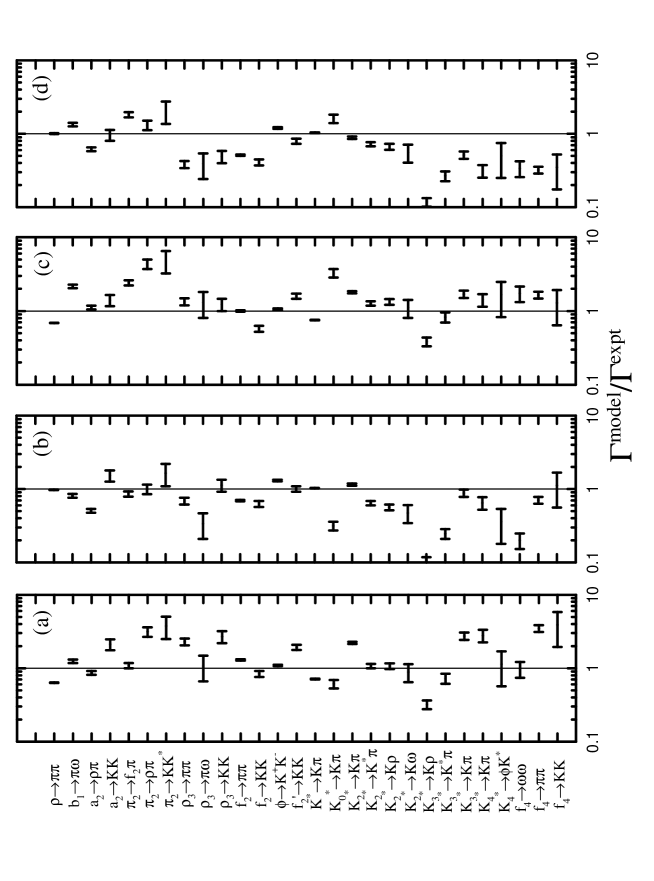
FIG. 2.: The ratio of decay model predictions for partial widths to the experimental values. The error bars only include the effects of experimental errors in the ratios. (a) and (b) correspond to the ${}^{3}P_{0}$ model using SHO wavefunctions and RPSN and KIPSN respectively (columns 3 and 4 of Table II). (c) and (d) correspond to the flux-tube breaking model using the RQM wavefunctions of Ref. [18] and RPSN and KIPSN respectively (columns 7 and 8 of Table II).

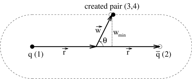
FIG. 3.: The position-space coordinates used in the flux-tube model. The cigar-shaped dashed line shows a possible surface of constant $\omega_{\rm min}$.

TABLE I.: Summary of $\xi(2220)$ measurements.

Experiment	Mass	Width	Production	Decays
	(MeV)	(MeV)
Mark III a	$2231\pm 8$	$21\pm 17$	$J/\psi\to\gamma\xi$	$BR(J/\psi\to\gamma\xi)\times BR(\xi\to K^{+}K^{-})$
				$=(4.2^{+1.7}_{-1.4}\pm 0.8)\times 10^{-5}$
				$BR(J/\psi\to\gamma\xi)\times BR(\xi\to K_{S}K_{S})$
				= $(3.1^{+1.6}_{-1.3}\pm 0.7)\times 10^{-5}$
				$BR(J/\psi\to\gamma\xi)\times BR(\xi\to\pi\pi)$
				$<2\times 10^{-5}$ (90% C.L.)
				$BR(J/\psi\to\gamma\xi)\times BR(\xi\to p\bar{p})$
				$<2\times 10^{-5}$ (90% C.L.)
DM2 b	$2230$ c	$26$ c	$J/\psi\to\gamma\xi$	$BR(J/\psi\to\gamma\xi)\times BR(\xi\to K^{+}K^{-})$
				$<2.3\times 10^{-5}$ (95% C.L.)
				$BR(J/\psi\to\gamma\xi)\times BR(\xi\to K_{S}K_{S})$
				$<1.6\times 10^{-5}$ (95% C.L.)
	$2197\pm 17$	$201\pm 51$	$J/\psi\to\gamma X$	$BR(J/\psi\to\gamma X)\times BR(X\to K_{S}K_{S})$
				$\simeq 1.5\times 10^{-4}$
BES d	$2233\pm 5$	$19\pm 11$	$J/\psi\to\gamma\xi$	$BR(J/\psi\to\gamma\xi)\times BR(\xi\to\pi^{+}\pi^{-})$
				$=(5.6^{+1.8}_{-1.6}\pm 1.4)\times 10^{-5}$
				$BR(J/\psi\to\gamma\xi)\times BR(\xi\to p\bar{p})$
				$=(1.5^{+0.6}_{-0.5}\pm 0.5)\times 10^{-5}$
				$BR(J/\psi\to\gamma\xi)\times BR(\xi\to K^{+}K^{-})$
				$=(3.3^{+1.6}_{-1.3}\pm 1.1)\times 10^{-5}$
				$BR(J/\psi\to\gamma\xi)\times BR(\xi\to K_{S}K_{S})$
				$=(2.7^{+1.1}_{-0.9}\pm 1.0)\times 10^{-5}$
LASS e	$2209^{+17}_{-15}\pm 10$	$60^{+107}_{-57}$	$K^{-}p\to K^{-}K^{+}\Lambda$
E147 f	$2230\pm 20$	$80\pm 30$	$\pi^{-}p\to K_{S}K_{S}n$
PS185 g	$2231$ c	$30$ c	$p\bar{p}\to K_{S}K_{S}$	$BR(\xi\to p\bar{p})\times BR(\xi\to K_{S}K_{S})$
				$<5.4\times 10^{-4}$ (3 S.D. J=4)

TABLE II.: Experimental and calculated widths (in MeV) of decays used in our global fit of the decay models’ parameters.

Decay	$\Gamma$(experiment)	${}^{3}P_{0}$		Flux-Tube Breaking		Flux-Tube Breaking
		(SHO)		(SHO)		(RQM)
		RPSN	KIPSN	RPSN	KIPSN	RPSN	KIPSN
$\gamma$		9.73	6.25	16.0	10.4	20.5	12.8
$\rho\to\pi\pi$	$151.2\pm 1.2$	96	148	93	148	104	152
$b_{1}(1235)\to\omega\pi$	$142\pm 8$	176	115	155	104	306	190
$a_{2}(1320)\to\rho\pi$	$75.0\pm 4.5$	65	38	67	40	84	46
$a_{2}(1320)\to K\bar{K}$	$5.2\pm 0.9$	11	8.0	11	8.5	7.3	5.0
$\pi_{2}(1670)\to f_{2}(1270)\pi$	$135\pm 11$	147	116	143	117	327	246
$\pi_{2}(1670)\to\rho\pi$	$74\pm 11$	232	74	226	74	323	97
$\pi_{2}(1670)\to K^{*}(892)\bar{K}+c.c.$	$10.1\pm 3.4$	38	17	37	17	49	21
$\rho_{3}(1690)\to\pi\pi$	$50.7\pm 5.5$	116	35	122	38	68	19
$\rho_{3}(1690)\to\omega\pi$	$34\pm 13$	36	11	39	13	45	13
$\rho_{3}(1690)\to K\bar{K}$	$3.4\pm 0.6$	9.2	3.8	9.7	4.2	4.2	1.7
$f_{2}(1270)\to\pi\pi$	$156.8\pm 3.2$	203	109	209	116	157	80
$f_{2}(1270)\to K\bar{K}$	$8.6\pm 0.8$	7.2	5.4	7.4	5.7	5.0	3.5
$\phi\to K^{+}K^{-}$	$2.17\pm 0.05$	2.37	2.83	2.28	2.80	2.30	2.60
$f_{2}^{\prime}(1525)\to K\bar{K}$	$61\pm 5$	117	61	118	64	98	49
$K^{*}(892)\to K\pi$	$50.2\pm 0.5$	36	52	34	51	38	52
$K_{0}^{*}(1430)\to K\pi$	$267\pm 36$	163	84	117	63	875	430
$K_{2}^{*}(1430)\to K\pi$	$48.9\pm 1.7$	108	56	112	60	88	43
$K_{2}^{*}(1430)\to K^{*}(892)\pi$	$24.8\pm 1.7$	27	16	27	17	31	18
$K_{2}^{*}(1430)\to K\rho$	$8.7\pm 0.8$	9.3	4.9	9.6	5.2	12	5.8
$K_{2}^{*}(1430)\to K\omega$	$2.9\pm 0.8$	2.6	1.4	2.6	1.4	3.2	1.6
$K_{3}^{*}(1780)\to K\rho$	$74\pm 10$	24	7.7	25	8.4	28	8.7
$K_{3}^{*}(1780)\to K^{*}(892)\pi$	$45\pm 7$	33	11	34	12	37	12
$K_{3}^{*}(1780)\to K\pi$	$31.7\pm 3.7$	87	28	92	30	54	16
$K_{4}^{*}(2045)\to K\pi$	$19.6\pm 3.8$	55	13	59	14	28	6.2
$K_{4}^{*}(2045)\to K^{*}(892)\phi$	$2.8\pm 1.4$	3.2	1.0	3.3	1.1	4.7	1.4
$f_{4}(2050)\to\omega\omega$	$54\pm 13$	53	11	54	11	94	18
$f_{4}(2050)\to\pi\pi$	$35.4\pm 3.8$	123	25	132	28	58	11
$f_{4}(2050)\to K\bar{K}$	$1.4\pm 0.7$	5.4	1.6	5.8	1.7	1.8	0.5

TABLE III.: Calculated partial decay widths (in MeV) for the ${}^{3}F_{4}$ $s\bar{s}$ state. We have calculated the widths of all kinematically allowed decays, but only show those partial widths that are $\geq 1$ MeV in at least one model. For this reason the total widths may not equal the sum of the partial widths shown. The subscripts on the decays refer to the $S$ and $L$ (see Appendix C) of the given partial wave — the $L$ is in spectroscopic notation ($S,P,D,F,G,H$).

Decay	${}^{3}P_{0}$		Flux-Tube Breaking		Flux-Tube Breaking
	(SHO)		(SHO)		(RQM)
	RPSN	KIPSN	RPSN	KIPSN	RPSN	KIPSN
$f^{\prime}_{4}\to[K\bar{K}]_{0,G}$	118	29	125	31	62	14
$f^{\prime}_{4}\to[K_{r}\bar{K}+c.c.]_{0,G}\leavevmode\leavevmode\hbox{${}^{\rm a}$}$	0.7	0.4	0.4	0.2	2.4	1.2
$f^{\prime}_{4}\to[K^{*}(892)\bar{K}+c.c.]_{1,G}$	107	27	115	29	112	26
$f^{\prime}_{4}\to[K^{*}(1410)\bar{K}+c.c.]_{1,G}\leavevmode\leavevmode\hbox{${}^{\rm b}$}$	1.7	0.9	0.8	0.4	5.0	2.4
$f^{\prime}_{4}\to[K_{1}(1270)\bar{K}+c.c.]_{1,F}\leavevmode\leavevmode\hbox{${}^{\rm c}$}$	6.4	2.8	7.0	3.1	10	4.2
$f^{\prime}_{4}\to[K_{1}(1270)\bar{K}+c.c.]_{1,H}\leavevmode\leavevmode\hbox{${}^{\rm c}$}$	1.3	0.6	1.4	0.6	3.7	1.5
$f^{\prime}_{4}\to[K_{1}(1400)\bar{K}+c.c.]_{1,F}\leavevmode\leavevmode\hbox{${}^{\rm c}$}$	14	6.4	15	7.0	29	12
$f^{\prime}_{4}\to[K_{2}^{*}(1430)\bar{K}+c.c.]_{2,F}$	15	7.0	16	7.7	35	15
$f^{\prime}_{4}\to[K^{*}(892)\bar{K}^{*}(892)]_{0,G}$	2.1	0.5	2.3	0.6	4.3	1.0
$f^{\prime}_{4}\to[K^{*}(892)\bar{K}^{*}(892)]_{2,D}$	181	44	184	46	312	72
$f^{\prime}_{4}\to[K^{*}(892)\bar{K}^{*}(892)]_{2,G}$	8.2	2.0	8.9	2.2	17	3.9
$f^{\prime}_{4}\to[\eta\eta]_{0,G}$	14	3.5	15	3.9	5.0	1.2
$f^{\prime}_{4}\to[\eta^{\prime}\eta]_{0,G}$	6.9	1.7	7.5	1.9	2.4	0.6
$f^{\prime}_{4}\to[\phi\phi]_{2,D}$	20	6.6	21	7.1	31	9.5
$\sum_{i}\Gamma_{i}$	498	132	522	142	633	166

TABLE IV.: Calculated partial decay widths (in MeV) for the ${}^{3}F_{2}$ $s\bar{s}$ state. We do not include a decay to $f_{0}(980)f_{0}(980)$ because we question its assignment as a ${}^{3}P_{0}$ $q\bar{q}$ meson. At a more likely mass for the ${}^{3}P_{0}$ $s\bar{s}$ meson, this decay is kinematically inaccessible. For other comments and notes, see Table III.

Decay	${}^{3}P_{0}$		Flux-Tube Breaking		Flux-Tube Breaking
	(SHO)		(SHO)		(RQM)
	RPSN	KIPSN	RPSN	KIPSN	RPSN	KIPSN
$f^{\prime}_{2}\to[K\bar{K}]_{0,D}$	51	12	47	12	101	23
$f^{\prime}_{2}\to[K_{r}\bar{K}+c.c.]_{0,D}$	2.9	1.5	0.9	0.5	25	12
$f^{\prime}_{2}\to[K^{*}(892)\bar{K}+c.c.]_{1,D}$	108	26	107	26	165	38
$f^{\prime}_{2}\to[K^{*}(1410)\bar{K}+c.c.]_{1,D}$	2.6	1.3	0.6	0.3	4.0	1.9
$f^{\prime}_{2}\to[K_{1}(1270)\bar{K}+c.c.]_{1,P}$	445	187	449	194	1072	426
$f^{\prime}_{2}\to[K_{1}(1270)\bar{K}+c.c.]_{1,F}$	25	11	27	12	41	16
$f^{\prime}_{2}\to[K_{1}(1400)\bar{K}+c.c.]_{1,P}$	14	6.3	15	6.9	29	12
$f^{\prime}_{2}\to[K_{1}(1400)\bar{K}+c.c.]_{1,F}$	0.8	0.4	1.0	0.4	$\sim 0$	$\sim 0$
$f^{\prime}_{2}\to[K_{2}^{*}(1430)\bar{K}+c.c.]_{2,P}$	54	24	55	25	112	47
$f^{\prime}_{2}\to[K_{2}^{*}(1430)\bar{K}+c.c.]_{2,F}$	9.6	4.3	10	4.7	22	9.1
$f^{\prime}_{2}\to[K^{*}(892)\bar{K}^{*}(892)]_{0,D}$	24	5.7	24	5.9	39	8.9
$f^{\prime}_{2}\to[K^{*}(892)\bar{K}^{*}(892)]_{2,D}$	14	3.3	14	3.4	23	5.1
$f^{\prime}_{2}\to[K^{*}(892)\bar{K}^{*}(892)]_{2,G}$	48	12	52	13	83	19
$f^{\prime}_{2}\to[K_{1}(1270)\bar{K}^{*}(892)+c.c.]_{1,P}$	99	40	102	42	209	79
$f^{\prime}_{2}\to[K_{1}(1270)\bar{K}^{*}(892)+c.c.]_{1,F}$	0.5	0.2	0.6	0.2	1.1	0.4
$f^{\prime}_{2}\to[K_{1}(1270)\bar{K}^{*}(892)+c.c.]_{2,P}$	33	13	34	14	70	26
$f^{\prime}_{2}\to[K_{1}(1270)\bar{K}^{*}(892)+c.c.]_{2,F}$	0.8	0.3	0.9	0.4	1.8	0.7
$f^{\prime}_{2}\to[\eta\eta]_{0,D}$	14	3.3	13	3.2	20	4.4
$f^{\prime}_{2}\to[\eta^{\prime}\eta]_{0,D}$	29	7.0	29	7.2	29	6.6
$f^{\prime}_{2}\to[f_{1}(1510)\eta]_{1,P}$	45	22	46	24	92	43
$f^{\prime}_{2}\to[f_{2}^{\prime}(1525)\eta]_{2,P}$	14	6.9	14	7.3	29	14
$f^{\prime}_{2}\to[\eta^{\prime}\eta^{\prime}]_{0,D}$	6.6	1.6	6.7	1.7	4.9	1.1
$f^{\prime}_{2}\to[\phi\phi]_{0,D}$	3.9	1.2	3.9	1.3	5.5	1.6
$f^{\prime}_{2}\to[\phi\phi]_{2,D}$	2.2	0.7	2.3	0.7	3.1	0.9
$f^{\prime}_{2}\to[\phi\phi]_{2,G}$	1.0	0.3	1.0	0.3	1.1	0.3
$\sum_{i}\Gamma_{i}$	1046	391	1058	406	2181	797

TABLE V.: Calculated partial decay widths (in MeV) for the $K_{4}^{*}(2045)$ state. For comments and additional notes, see Table III.

Decay	Experiment	${}^{3}P_{0}$
		(SHO)
		RPSN	KIPSN
$K_{4}^{*}(2045)\to[K\pi]_{0,G}$	$19.6\pm 3.8$	55	13
$K_{4}^{*}(2045)\to[K\rho]_{1,G}$		19	4.4
$K_{4}^{*}(2045)\to[Kb_{1}(1235)]_{1,F}$		4.9	2.2
$K_{4}^{*}(2045)\to[Ka_{1}(1260)]_{1,F}$		1.3	0.6
$K_{4}^{*}(2045)\to[Ka_{2}(1320)]_{2,F}$		2.2	1.0
$K_{4}^{*}(2045)\to[K^{*}(892)\pi]_{1,G}$		23	5.5
$\!\!\!\left.\begin{array}[]{l}K_{4}^{*}(2045)\to[K^{*}(892)\rho]_{2,D}\\ K_{4}^{*}(2045)\to[K^{*}(892)\rho]_{2,G}\end{array}\right\}$	$18\pm 10$ a	$\begin{array}[]{c}76\\ 2.1\end{array}$	$\begin{array}[]{c}18\\ 0.5\end{array}$
$K_{4}^{*}(2045)\to[K_{1}(1270)\pi]_{1,F}$		1.6	0.7
$K_{4}^{*}(2045)\to[K_{1}(1400)\pi]_{1,F}$		5.3	2.6
$K_{4}^{*}(2045)\to[K_{2}^{*}(1430)\pi]_{2,F}$		5.2	2.6
$K_{4}^{*}(2045)\to[K\eta^{\prime}]_{0,G}$		3.3	0.9
$K_{4}^{*}(2045)\to[K\omega]_{1,G}$		6.0	1.4
$K_{4}^{*}(2045)\to[K\phi]_{1,G}$		1.1	0.4
$K_{4}^{*}(2045)\to[Kh_{1}(1170)]_{1,F}$		2.9	1.3
$K_{4}^{*}(2045)\to[Kf_{2}(1270)]_{2,F}$		1.3	0.6
$K_{4}^{*}(2045)\to[K^{*}\eta]_{1,G}$		4.9	1.4
$K_{4}^{*}(2045)\to[K^{*}(892)\omega]_{2,D}$		24	5.7
$K_{4}^{*}(2045)\to[K^{*}(892)\phi]_{2,D}$	$2.8\pm 1.4$	3.2	1.0
$\sum_{i}\Gamma_{i}$	$198\pm 30$	247	65

TABLE VI.: Calculated partial decay widths (in MeV) for the $f_{4}(2050)$ state. For comments and additional notes, see Table III.

Decay	Experiment	${}^{3}P_{0}$
		(SHO)
		RPSN	KIPSN
$f_{4}(2050)\to[\pi\pi]_{0,G}$	$35.4\pm 3.8$	123	25
$f_{4}(2050)\to[\pi\pi(1300)]_{0,G}$		3.9	1.9
$f_{4}(2050)\to[\pi a_{1}(1260)]_{1,F}$		18	7.5
$f_{4}(2050)\to[\pi a_{2}(1320)]_{2,F}$		44	19
$f_{4}(2050)\to[\pi\pi_{2}(1670)]_{2,D}$		2.1	1.8
$f_{4}(2050)\to[\rho\rho]_{0,G}$		1.9	0.4
$f_{4}(2050)\to[\rho\rho]_{2,D}$		159	33
$f_{4}(2050)\to[\rho\rho]_{2,G}$		7.3	1.5
$f_{4}(2050)\to[\eta\eta]_{0,G}$		3.2	0.9
$f_{4}(2050)\to[\eta\eta^{\prime}]_{0,G}$		1.0	0.3
$f_{4}(2050)\to[\eta f_{2}(1270)]_{2,F}$		1.1	0.5
$\!\!\!\left.\begin{array}[]{l}f_{4}(2050)\to[\omega\omega]_{2,D}\\ f_{4}(2050)\to[\omega\omega]_{2,G}\end{array}\right\}$	$54\pm 13$ b	$\begin{array}[]{c}50\\ 2.0\end{array}$	$\begin{array}[]{c}10\\ 0.4\end{array}$
$f_{4}(2050)\to[K\bar{K}]_{0,G}$	$1.4\pm 0.7$	5.4	1.6
$f_{4}(2050)\to[K\bar{K}^{*}(892)+c.c.]_{1,G}$		2.7	0.8
$f_{4}(2050)\to[K\bar{K}_{1}(1270)+c.c.]_{1,F}$		2.3	1.2
$f_{4}(2050)\to[K^{*}(892)\bar{K}^{*}(892)]_{2,D}$		7.3	2.1
$\sum_{i}\Gamma_{i}$	$198\pm 30$	435	109

TABLE VII.: Calculated total decay widths (in MeV) for the ${}^{3}F_{2}$ and ${}^{3}F_{4}$ $s\bar{s}$ states for different values of $\beta$.

$\beta$ (MeV)	$\gamma$	$\Gamma(^{3}F_{2})$	$\Gamma(^{3}F_{4})$
RPSN
350	7.42	590	540
400	9.73	1046	498
450	12.0	1549	429
481a	13.4	1841	388
KIPSN
350	5.16	256	170
371a	5.60	309	152
400	6.25	391	132
450	7.39	534	104

REFERENCES

- [1] The Mark III Collaboration, Baltrusaitis et al, Phys. Rev. Lett. 56, 107 (1986).
- [2] R.M. Barnett, G. Senjanović, L. Wolfenstein, and D. Wyler, Phys. Lett. 136B, 191 (1984); R.S.Willey, Phys. Rev. Lett. 52, 585 (1984); H.E. Haber and G.L. Kane, Phys. Lett. 135B, 196 (1984).
- [3] M.P. Shatz, Phys. Lett. 138B, 209 (1984).
- [4] S. Pakvasa, M. Suzuki, and S.F. Tuan, Phys. Rev. D31, 2378 (1985); Kuang-Ta Chao, Phys. Rev. Lett. 60, 2579 (1988); Commun. Theor. Phys., 3 757 (1984).
- [5] S. Pakvasa, M. Suzuki, and S.F. Tuan, Phys. Lett. 145B, 135 (1984).
- [6] S. Ono, Phys. Rev. D35, 944 (1987).
- [7] A. Le Yaouanc, L. Oliver, O. Pène, J.-C. Raynal, Z. Phys. C28, 309 (1985); M.S. Chanowitz and S.R. Sharpe, Phys. Lett. 132B, 413 (1983).
- [8] B.F.L. Ward, Phys. Rev. D31, 2849 (1985); erratum ibid D32, 1260 (1985); Qi-xing Shen, Hong Yu, Phys. Lett. B247, 418 (1990); Kuang-Ta Chao, Beijing University Report PUTP-94-26 hep-ph/9502408.
- [9] S. Godfrey, R. Kokoski, and N. Isgur, Phys. Lett. 141B, 439 (1984).
- [10] DM2 Collaboration, J.E. Augustin et al., Phys. Rev. Lett. 60, 2238 (1988).
- [11] S. Jin, talk given at the International Workshop on Hadron Physics at Electron-Positron Colliders, Beijing, October 14-17 (1994).
- [12] The LASS Collaboration, D. Aston et al., Nucl. Phys. B301, 525 (1988); Phys. Lett. B215, 199 (1988).
- [13] B.V. Bolonkin et al., Nucl. Phys. B309, 426 (1988).
- [14] P.D. Barnes et al., Phys. Lett. B309, 469 (1988).
- [15] The model of meson decay was first discussed by A. Le Yaouanc, L. Oliver, O. Pène and J.-C. Raynal, Phys. Rev. D 8, 2223 (1973). For further references to the model, see R. Kokoski, Ph.D thesis, University of Toronto, 1984.
- [16] W. Roberts and B. Silvestre-Brac, Few-Body Systems, 11, 171 (1992).
- [17] R. Kokoski and N. Isgur, Phys. Rev. D 35, 907 (1987).
- [18] S. Godfrey and N. Isgur, Phys. Rev. D32, 189 (1985).
- [19] P. Geiger and E.S. Swanson Phys. Rev. D50, 6855 (1994).
- [20] N. Isgur, private communication.
- [21] The Particle Data Group, L. Montanet et al., Phys. Rev. D50 1173 (1994).
- [22] UKQCD Collaboration, G.S. Bali et al., Phys. Lett. B309, 378 (1993).
- [23] J. Sexton, A. Vaccarino, and D. Weingarten, hep-lat/9510022.
- [24] Cameron Hayne and Nathan Isgur, Phys. Rev. D 25, 1944 (1982).
- [25] Suh Urk Chung, “Spin Formalisms”, Technical Note CERN 71-8, CERN, 1971; Jeffrey D. Richman, “An Experimenter’s Guide to the Helicity Formalism”, Technical Note CALT-68-1148, California Institute of Technology, 1984; M. Jacob and G.C. Wick, Ann. Phys. 7 404 (1959).
- [26] Stephen Wolfram, “Mathematica: A System for Doing Mathematics by Computer”, second edition, Addison-Wesley, 1991. For the flux-tube breaking model of meson decay, fortran code was created using the Mathematica packages Format.m and Optimize.m, written by M. Sofroniou and available from MathSource (URL: http://www.wri.com/).
- [27] G. Peter Lepage, J. Comp. Phys. 27, 192 (1978); G. Peter Lepage, “VEGAS - An Adaptive Multi-dimensional Integration Program”, Cornell University Technical Note CLNS-80/447, 1980.