JHU-TIPAC-95022
hep-ph/9508219

THE STRONG COUPLING AND THE BOTTOM MASS

IN SUPERSYMMETRIC GRAND UNIFIED THEORIES

DAMIEN PIERCE

Department of Physics and Astronomy

Johns Hopkins University

3400 N. Charles Street

Baltimore, Maryland 21218, USA

E-mail: pierce@planck.pha.jhu.edu

We apply the full one-loop corrections to the masses, gauge couplings, and Yukawa couplings in the minimal supersymmetric standard model. We focus on predictions for the strong coupling and the bottom-quark pole mass in the context of SU(5) supersymmetric grand unification. We discuss our results in both the small and large $\tan\beta$ regimes. We demonstrate that the finite (non-logarithmic) corrections to the weak mixing angle are essential in determining $\alpha_{s}$ and $m_{b}$ when some superpartner masses are light. Minimal SU(5) predicts acceptable $\alpha_{s}$ and $m_{b}$ only at small $\tan\beta$ with SUSY masses of $\cal O$(TeV). The missing doublet model accommodates gauge and Yukawa coupling unification for small or large $\tan\beta$, and for any SUSY mass scale. In the large $\tan\beta$ case, the bottom mass is acceptable only if the Higgsino mass parameter $\mu$ is positive.

1 Introduction

This talk is organized as follows. First, we briefly discuss the supersymmetric standard model, in order to introduce the parameter space we are considering. Next, we discuss the prediction for the strong coupling constant and the bottom pole mass with and without including GUT threshold effects, in the small $\tan\beta$ case. Lastly we discuss our results in the large $\tan\beta$ regime.

The minimal supersymmetric model is attractive in that it solves the hierarchy problem. It does this, however, at the expense of doubling the number of degrees of freedom of the standard model. This is problematic, as supersymmetry must be broken and hence the number of new parameters needed to describe the model is in general quite large. An organizing principle is needed in order to reduce the number of parameters. In a minimal supergravity scenario the number of supersymmetry breaking parameters needed to describe the supersymmetric model are few: a universal scalar mass $M_{0}$, a universal gaugino mass $M_{1/2}$, a universal trilinear scalar coupling $A_{0}$, and a bilinear scalar coupling $B$. In addition there is a supersymmetric Higgs mass term, $\mu$. Given values for these five parameters at the GUT scale, we use the renormalization group equations ^? (RGE’s) to determine the various particle masses and couplings at the weak scale. For a large top-quark mass, one of the Higgs boson masses is driven negative, and the radiative breaking of $SU(2)\times U(1)$ symmetry becomes manifest. The Higgs bosons obtain vev’s $v_{1}$ and $v_{2}$, and we can determine the $Z$-boson mass. In practice it is convenient to assume electroweak symmetry breaks radiatively and to take $M_{Z}$ as an input parameter, as well as the ratio of vev’s $\tan\beta\equiv v_{2}/v_{1}$. We then determine $\mu^{2}$ and $B$ from the symmetry breaking conditions. To summarize, then, the supersymmetric model is parametrized by

$$M_{0},\ \ M_{1/2},\ \ A_{0},\ \ \tan\beta,\ \ {\rm sign}(\mu).$$

The exact one-loop corrections to the masses, gauge couplings and Yukawa couplings of the minimal supersymmetric model are described in Ref. [2]. These corrections are essential ingredients for accurate tests of grand unification. They allow one to extract the underlying $\overline{\it DR}$ parameters from a given set of measured observables. The $\overline{\it DR}$ parameters can then be run up to a high scale to explore the consequences of different unification hypotheses.

Alternatively, the radiative corrections can be used to translate various limits into excluded regions of the $\overline{\it DR}$ parameter space. This is illustrated in Fig. 1, where we show the excluded region of the $M_{0},\ M_{1/2}$ parameter space at the one-loop level, from current experimental constraints.

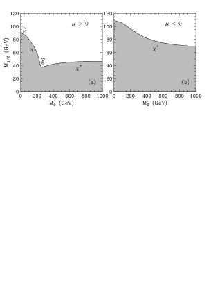
Figure 1: Excluded region (shaded) of the $M_{0},\ M_{1/2}$ plane, for $\tan\beta=2,\ m_{t}=175$ GeV, $A_{0}=0$, and $\alpha_{s}=0.117$. All masses are evaluated at one-loop. The symbols indicate which experimental constraint is relevant: $\chi^{+}\Rightarrow m_{\chi^{+}}>47$ GeV; $\tilde{g}\Rightarrow m_{\tilde{g}}>125$ GeV; $\tilde{\nu}\Rightarrow m_{\tilde{\nu}}>42$ GeV; $h\Rightarrow m_{h}>60$ GeV.

In the following, we treat all supersymmetric threshold corrections in a complete one-loop analysis. Our work stands in contrast to most previous studies, which are based on the “leading logarithm approximation.” For the gauge coupling threshold corrections, this approximation involves taking the standard-model value of $\sin^{2}\theta_{W}$ and adding the logarithmic parts of the SUSY threshold corrections. The approximation works well if all of the SUSY particle masses are much greater than $M_{Z}$, in which case the decoupling theorem implies that the finite effects of the SUSY particles are negligible for all low-energy observables.

However, in realistic models it is not unusual for the supersymmetric spectrum to contain light particles of order the $Z$-mass. In this case the leading logarithm approximation breaks down. This is illustrated in Fig. 2, where we compare the value of $\alpha_{s}$ and $m_{b}$ in the leading logarithm approximation (LLA) with the value obtained in the full calculation. In this talk we use the full set of one-loop radiative corrections to evaluate the $\overline{\it DR}$ gauge and Yukawa couplings. The $\overline{\it DR}$ couplings serve as the boundary conditions for the two-loop gauge and Yukawa coupling renormalization group equations, which determine the couplings at very high scales.

Figure 2: Comparison of (a) $\alpha_{s}$ and (b) $m_{b}$ in the leading logarithm approximation (LLA) versus the full one-loop calculation, for $M_{0}=60$ GeV, $\tan\beta=2,\ m_{t}=175$ GeV, $A_{0}=0$, and $\mu>0$. The dashed line shows the result if the non-universal corrections are neglected.

In what follows, we have converted the strong coupling to the $\overline{\it MS}$ scheme so that by $\alpha_{s}$ we refer to the standard $\overline{\it MS}$ value evaluated at the scale $M_{Z}$. By $m_{b}$ we refer to the bottom-quark pole mass.

2 Small $\tan\beta$

As a reference point, we show in Fig. 3 contours of $m_{b}$ and $\alpha_{s}$ in the $M_{0},\ M_{1/2}$ plane, with no GUT thresholds, $\tan\beta=2$, $m_{t}=175$ GeV, and $A_{0}$=0. We confine our attention to the region of the theory which is more natural, i.e. to the region where the superpartner masses are less than about 1 TeV. We find the strong coupling is large ($\alpha_{s}>0.127$) compared to the PDG value ^? $\alpha_{s}=0.117\pm 0.005$. Similarly, the bottom mass is quite large ($m_{b}>6$ GeV), far outside the preferred region which we take to be $4.7<m_{b}<5.2$ GeV.

Figure 3: Contours of $\alpha_{s}$ (solid lines) and $m_{b}$ (dashed) in the $M_{0}$, $M_{1/2}$ plane, with $\tan\beta=2$, $m_{t}=175$ GeV, and $A_{0}=0$. The upper left hand corners are excluded on cosmological grounds (charged LSP) and the lower shaded regions are excluded by particle searches. The $m_{b}$ contours are labeled in GeV.

The experimental uncertainty in the determination of $\alpha_{s}$ is primarily due to the uncertainty in determining the electromagnetic coupling at the $Z$-scale. We use the value recently determined by Eidelman and Jegerlehner ^?. The one-sigma uncertainty in our input $\alpha_{EM}(M_{Z})$ results in a one-sigma uncertainty in our output $\alpha_{s}$ of about $\pm 0.001$, and an uncertainty of typically 0.07 GeV in our bottom mass prediction. Martin and Zeppenfeld ^? and Swartz ^? have also performed analyses to determine $\alpha_{EM}(M_{Z})$. The central value for $\alpha_{s}$ increases by about 0.001 if we use the value of $\alpha_{\rm EM}(M_{Z})$ as determined by Martin and Zeppenfeld, and it increases by about 0.002 if we use the value of $\alpha_{EM}(M_{Z})$ from Swartz.

The bottom mass is reduced if we go further into the small $\tan\beta$ region, due to the large top-quark Yukawa coupling in the bottom mass renormalization group equation. We consider the case where the top Yukawa is as large as possible; we set $\lambda_{t}(M_{\rm GUT})=3$, which is on the verge of the nonperturbative regime. In this case we will obtain the smallest possible bottom mass. As seen in Fig. 4, for $m_{t}=180$ GeV the bottom mass is less than 5.2 GeV and the strong coupling is less than 0.127 only if the squark masses are in the TeV region.

Figure 4: The bottom-quark mass and $\alpha_{s}$ vs. $m_{t}$ for the case of no GUT-scale thresholds, for various values of $\tan\beta$, with $A_{0}=0$, $\mu>0$, and $\lambda_{t}(M_{\rm GUT})=3$. The circles on the right (solid) leg in each pair of lines corresponds to $M_{1/2}$ equal to (from top to bottom) 60, 100, 200, 500 GeV, with $M_{0}$ fixed at 100 GeV. The circles on the left (dashed) leg corresponds to $M_{0}$ equal to 100, 200, 400 and 1000 GeV, with $M_{1/2}=100$ GeV. The horizontal dot-dashed lines indicate $m_{b}=5.2$ GeV and $\alpha_{s}=0.127$. The $\times$’s mark points with one-loop Higgs mass $m_{h}<60$ GeV.

If we consider particular GUT models, we can determine whether the GUT threshold corrections to the gauge and Yukawa couplings can help improve the situation. We parametrize the GUT threshold corrections by $\varepsilon_{g}$ and $\varepsilon_{b}$, where

$$g_{3}(M_{\rm GUT})=g_{\rm GUT}(M_{\rm GUT})\left(1+\varepsilon_{g}\right)\ ,$$

$$\lambda_{b}(M_{\rm GUT})=\lambda_{\tau}(M_{\rm GUT})\left(1+\varepsilon_{b}\right)\ ,$$

where $\lambda_{b}$ and $\lambda_{\tau}$ are the $b$- and $\tau$-Yukawa couplings, and $M_{\rm GUT}$ is defined as the scale at which $g_{1}$ and $g_{2}$ meet, $g_{\rm GUT}\equiv g_{1}(M_{\rm GUT})=g_{2}(M_{\rm GUT})$. A smaller value of $\alpha_{s}$ requires $\varepsilon_{g}<0$. In the small $\tan\beta$ region the bottom mass is tightly correlated with the value of the strong coupling. Hence, setting $\varepsilon_{g}<0$ reduces both $\alpha_{s}$ and $m_{b}$. In fact, the bottom mass is an order of magnitude more sensitive to $\varepsilon_{g}$ than to $\varepsilon_{b}$. In what follows we examine the GUT corrections in two SU(5) GUT models.

Figure 5: Contours of the smallest possible $\alpha_{s}$ (solid lines) and $m_{b}$ (dashed) consistent with nucleon decay in (a) minimal SU(5), and (b) missing doublet SU(5), with $m_{t}=175$ GeV, $A_{0}=0$ and $\mu>0$. In (a) $\lambda_{t}(M_{\rm GUT})=3$ ($\tan\beta\simeq 1.4$) and in (b) $\tan\beta=2$. The shaded regions are phenomenologically excluded. The $m_{b}$ contours are labeled in GeV.

Figure 6: Contours of $\alpha_{s}$ (solid) and $m_{b}$ (dashed, labeled in GeV) with no GUT thresholds, $m_{t}=175$ GeV, $A_{0}=0$ and $\tan\beta=30$.

Figure 7: Contours of $\alpha_{s}$ (solid) and $m_{b}$ (dashed, labeled in GeV) in missing doublet SU(5), with $m_{t}=175$ GeV, $A_{0}=0$ and $\tan\beta=30$.

In the minimal SU(5) model ^?, the gauge coupling threshold correction $\varepsilon_{g}^{\prime}$ is given by ^?

$$\varepsilon^{\prime}_{g}\ =\ {3g_{\rm GUT}^{2}\over 40\pi^{2}}\,\log\left(M_{H_{3}}\over M_{\rm GUT}\right)\ ,$$ (1)

where $M_{H_{3}}$ is the mass of the color-triplet Higgs particle that mediates nucleon decay. From this expression, we see that $\varepsilon^{\prime}_{g}<0$ whenever $M_{H_{3}}<M_{\rm GUT}$. However, $M_{H_{3}}$ is bounded from below by proton decay experiments. The $M_{H_{3}}$ mass limit is of the form ^?

$$M_{H_{3}}>{\cal M}\ {|1+y^{tK}|\over\sin 2\beta}f(\tilde{w},\tilde{d},\tilde{u},\tilde{e})$$

where ${\cal M}$ is a nuclear matrix element, $y^{tK}$ parametrizes the amount of third generation mixing, and $f$ is a function of the wino, squark and slepton masses.

For the conservative choices ${\cal M}=0.003$ GeV³ and $|1+y^{tK}|=0.4$ we find that $M_{H_{3}}^{\rm min}>M_{\rm GUT}$ unless $M_{0}>500$ GeV and $M_{1/2}\ll M_{0}$. Thus, in most of the parameter space, $\varepsilon_{g}^{\prime}>0$. For this reason, in minimal SU(5), $\alpha_{s}$ is typically even larger than in the case of no GUT thresholds, as illustrated in Fig. 5(a). In order to obtain the smallest possible $\alpha_{s}$ and $m_{b}$, we have set $\lambda_{t}(M_{\rm GUT})=3$ in Fig. 5(a). Thus we end up with rather small values for $\tan\beta$ ($\sim 1.3$-1.6), and the Higgs mass constraint rules out a large part of parameter space. Only in the region $M_{0}\gg M_{1/2}$, where the proton decay amplitude is suppressed, is the strong coupling reduced relative to the case with no GUT thresholds. The smallest value of $\alpha_{s}$ occurs in this region, a somewhat large value of 0.124. The bottom-quark mass is similarly on the high side of the preferred region. We have applied the most favorable Yukawa correction $\varepsilon_{b}$ given in Wright ^?, subject to Yukawa coupling perturbativity constraints (see Bagger et al. ^?).

The missing-doublet model is an alternative SU(5) theory in which the heavy color-triplet Higgs particles are split naturally from the light Higgs doublets ^?. In this model the GUT gauge threshold correction is given by ^?

$$\varepsilon_{g}^{\prime\prime}\ =\ {3g_{\rm GUT}^{2}\over 40\pi^{2}}\,\Biggl{\{}\log\left(M_{H_{3}}^{\rm eff}\over M_{\rm GUT}\right)-{25\over 2}\log 5+15\log 2\Biggr{\}}\ \simeq\ \varepsilon^{\prime}_{g}-4\%\ .$$ (2)

Thus, for fixed $M_{H_{3}}$, the missing-doublet model has the same threshold correction as the minimal SU(5) model, minus 4%. In eq. (2), $M_{H_{3}}^{\rm eff}$ is the effective mass that enters into the proton decay amplitude, so the bounds on $M_{H_{3}}$ in the minimal SU(5) model also apply to $M_{H_{3}}^{\rm eff}$ in the missing-doublet model.

The large negative correction in eq. (2) is due to the mass splitting in the 75 representation, and gives rise to much smaller values for $\alpha_{s}$ and $m_{b}$. This is illustrated in Fig. 5(b), where we show contours of $\alpha_{s}$ and $m_{b}$ in the $M_{0},\ M_{1/2}$ plane, with $M_{H_{3}}^{\rm eff}=M_{H_{3}}^{\rm min}$, at $\tan\beta=2$. We find (even without going into the far infrared top Yukawa fixed point region) values of both the strong coupling and the bottom mass near their central values.

3 Large $\tan\beta$

Again, as a reference point, we show in Fig. 6 the strong coupling and bottom mass prediction with no GUT corrections, for $A_{0}=0,\ m_{t}=175$ GeV, at $\tan\beta=30$. The $\alpha_{s}$ predictions are not significantly different from the small $\tan\beta$ case. The bottom mass is significantly influenced by the large finite corrections ^?,

$${\Delta m_{b}\over m_{b}}\sim-{\mu\tan\beta\over 16\pi^{2}m_{\tilde{q}}^{2}}\left({8\over 3}g_{3}^{2}m_{\tilde{g}}+\lambda_{t}^{2}A_{t}\right)\ ,$$

so much so, that for the case $\mu<0$ the bottom mass is hopelessly large. However, these help to reduce $m_{b}$ when $\mu>0$. Even so, we see in Fig. 6(a) that $m_{b}>5.5$ GeV. GUT threshold corrections are needed to reduce both $\alpha_{s}$ and $m_{b}$ further.

In minimal SU(5) the proton decay rate is enhanced at large $\tan\beta$, so the triplet Higgs mass $M_{H_{3}}$ is forced to be quite large. Hence, we have a large and positive GUT correction $\varepsilon_{g}^{\prime}$ (Eq. (1)) which forces the strong coupling to unacceptably large values ($>$$\sim$0.14). Hence we conclude that minimal SU(5) is ruled out at large $\tan\beta$.

In the missing doublet model the large triplet Higgs mass correction is adequately compensated by the constant $-4\%$ correction of Eq. (2). As shown in Fig. 7, this cancellation results in near central values for $\alpha_{s}$ and $m_{b}$. However, $\mu>0$ is clearly required when $\tan\beta$ becomes large, as the large finite corrections have the wrong sign in the $\mu<0$ case, yielding values of $m_{b}$ which are unacceptably large.

4 Conclusion

In this talk we have presented results from a complete calculation of the one-loop corrections to the masses, gauge, and Yukawa couplings in the MSSM. We have seen that such a calculation allows us to reliably investigate various unified models to determine whether they are compatible with current experimental data. In particular, we found that the finite SUSY corrections, which are neglected in the leading logarithm approximation, can substantially increase the prediction for $\alpha_{s}$ and $m_{b}$ when some of the SUSY partner masses are lighter than or of order $M_{Z}$.

For small $\tan\beta$, we found that in the minimal SU(5) model, $\alpha_{s}$ was somewhat large ($\alpha_{s}>0.124$ with $m_{\tilde{q}}<1$ TeV) and $m_{b}$ was larger than 5 GeV. The missing doublet model gave much lower values of $\alpha_{s}$ and $m_{b}$, near their central values.

For large $\tan\beta$, the minimal SU(5) model GUT threshold correction became quite large and positive, and this resulted in unacceptably large values of the strong coupling ($\alpha_{s}\raise 1.29167pt\hbox{$>$\kern-7.5pt\lower 4.30554pt\hbox{$\sim$}}0.14$). The missing doublet model, on the other hand, had no trouble in accomodating the central values of the strong coupling and $m_{b}$. The values of $m_{b}$ were largely determined by important finite corrections, and we required $\mu>0$ in order for these corrections to result in acceptably small values of the bottom-quark mass.

5 Acknowledgements

I would like to thank my collaborators Jonathan Bagger and Konstantin Matchev. This work was supported by the U.S. National Science Foundation under grant NSF-PHY-9404057.

6 References

References

- [1] M.E. Machacek and M.T. Vaughn, Nucl. Phys. B 222 (1983) 83; ibid. 236 (1984) 221; ibid. 249 (1985) 70; I. Jack, Phys. Lett. B 147 (1984) 405; S. Martin, M. Vaughn, Northeastern preprint NUB-3081-93-TH (1993); Y. Yamada Phys. Rev. D 50 (1994) 3537; I. Jack and D.R.T. Jones, Phys. Lett. B 333 (1994) 372.
- [2] J. Bagger, K. Matchev, D. Pierce, and R. Zhang, to appear.
- [3] P. Chankowski, Z. Płuciennik and S. Pokorski, Nucl. Phys. B 439 (1995) 23.
- [4] Particle Data Group Review of Particle Properties, Phys. Rev. D 50 (1994) 1.
- [5] S. Eidelman and F. Jegerlehner, preprint PSI-PR-95-1, (1995).
- [6] A.D. Martin and D. Zeppenfeld, Phys. Lett. B 345 (1995) 558.
- [7] M. Swartz, SLAC preprint SLAC-PUB-6710 (1994).
- [8] S. Dimopoulos and H. Georgi, Nucl. Phys. B 193 (1981) 150; N. Sakai, Z. Phys. C 11 (1981) 153.
- [9] M.B. Einhorn and D.R.T. Jones, Nucl. Phys. B 196 (1982) 475; I. Antoniadis, C. Kounnas and K. Tamvakis, Phys. Lett. B 119 (1982) 377.
- [10] J. Hisano, H. Murayama and T. Yanagida, Nucl. Phys. B 402 (1993) 46.
- [11] B. Wright, Madison preprint MAD-PH-510 (1994).
- [12] J. Bagger, K. Matchev and D. Pierce, Phys. Lett. B 348 (1995) 443.
- [13] A. Masiero, D.V. Nanopoulos, K. Tamvakis and T. Yanagida, Phys. Lett. B 115 (1982) 380; B. Grinstein, Nucl. Phys B 206 (1982) 387.
- [14] K. Hagiwara and Y. Yamada, Phys. Rev. Lett. 70 (1993) 709; see also Y. Yamada, Z. Phys. C 60 (1993) 83.
- [15] L.J. Hall, R. Rattazzi and U. Sarid, Phys. Rev. D50 (1994) 7048; M. Carena, M. Olechowski, S. Pokorski and C.E.M. Wagner, Nucl. Phys. B426 (1994) 269; R. Hempfling, Z. Phys. C63 (1994) 309.