Abstract

The extraction of the CKM angle $\alpha$ from the asymmetry in $B^{0}\to\pi^{+}\pi^{-}$ vs ${\bar{B}^{0}}\to\pi^{+}\pi^{-}$ suffers from a currently unknown penguin contribution. Experimentally, one can determine the magnitude and phase of the CP asymmetry from a time-dependent analysis of tagged events, and the average rate for $B^{0}$ and $\bar{B}^{0}$ decays to $\pi^{+}\pi^{-}$ from untagged events. These measurements, together with the magnitudes and relative phase of the tree and penguin diagrams, can in principle completely determine $\alpha$, free of discrete ambiguities. We perform an error analysis on $\alpha$ given assumptions on the values and uncertainties of both the measurements and theoretical inputs.

1 Introduction

The unitarity of the CKM matrix corresponds to six independent conditions between

the CKM matrix elements[1]. Geometrically, these conditions can be visualized as triangles formed by the appropriate CKM matrix element combinations. The condition on the $d$ and $b$ rows, $\sum_{q=u,c,t}V_{qd}V_{qb}^{*}=0$, results in the CKM triangle shown in Fig. 1. If CP violation occurs via the CKM matrix, this triangle will have non-zero area. The three angles in this triangle, known as $\alpha$, $\beta$ and $\gamma$, can be extracted via CP asymmetries: the angle $\beta$ from the decay $B^{0}\to J/\psi K_{s}$[2], the angle $\alpha$ from the decay $B^{0}\to\pi^{+}\pi^{-}$[3] and the angle $\gamma$ from the decays $B_{s}\to D_{s}K$[4] and $B^{\pm}\to D^{0}K^{\pm}$[5].

Figure 1: The $d,b$ CKM triangle

The amplitude for $B\to\pi\pi$ is dominated by the tree process $b\to uW,W\to d\bar{u}$, which has a weak phase $\gamma$. If this were the only contribution, the CP asymmetry in $B^{0}\to\pi^{+}\pi^{-}$ would cleanly measure $\sin(2\beta+2\gamma)=-\sin(2\alpha)$. However, there may be significant contributions from the penguin process $b\to dg$. This process has a weak phase $-\beta$ and therefore results in a distortion of the CP asymmetry. Any interpretation of the CP asymmetry in $B^{0}\to\pi^{+}\pi^{-}$ must therefore account for the possibility of a penguin contribution.

Gronau and London[3] have shown that the penguin contributions can be isolated by applying an isospin analysis to the decays $B^{0}\to\pi^{+}\pi^{-}$, $B^{+}\to\pi^{+}\pi^{0}$ and $B^{0}\to\pi^{0}\pi^{0}$. Aleksan, Gaidot, and Vaisseur[6] have estimated that this analysis typically results in a 60% increase in the uncertainty on $\sin(2\alpha)$ relative to the ideal case where only the tree diagram need be considered. While feasible for an experiment at an $e^{+}e^{-}$ collider, this analysis is of no use to an experiment at a hadron collider, given that it is very unlikely that the mode $B^{0}\to\pi^{0}\pi^{0}$ will ever be reconstructed in such an environment.

Silva and Wolfenstein have shown[7] that $\alpha$ can be determined from the CP asymmetry in $B^{0}\to\pi^{+}\pi^{-}$, the relative rates for $B^{0}\to\pi^{+}\pi^{-}$ and $B^{0}\to K^{+}\pi^{-}$, and assuming SU(3) symmetry and factorization. Some complications are the possibility of final state phase shifts, and electroweak penguins that invalidate the SU(3) correspondence[8].

We present herein an analysis of the expected uncertainty on $\alpha$, and the number of discrete solutions, given a measurement of the time-dependent asymmetry between $B^{0}\to\pi^{+}\pi^{-}$ and ${\bar{B}^{0}}\to\pi^{+}\pi^{-}$, a measurement of the average branching ratio for $B^{0}$ and ${\bar{B}^{0}}$ decays to $\pi^{+}\pi^{-}$, and constraints on the magnitudes and relative phase of the tree and penguin diagrams.

2 CP violation in $B^{0}\to\pi^{+}\pi^{-}$

The mathematical expression of the CP asymmetry in the decay $B^{0}\to\pi^{+}\pi^{-}$ can be found in numerous places in the literature. Here we follow the exposition of Gronau[9].

In general, the two physical states $B_{L}$ and $B_{H}$ are given in terms of the strong eigenstates $B^{0}$ and $\bar{B}^{0}$ via

$$|B_{L}\rangle=p|B^{0}\rangle+q|{\bar{B}^{0}}\rangle$$ (2.1)

$$|B_{H}\rangle=p|B^{0}\rangle-q|{\bar{B}^{0}}\rangle$$ (2.2)

If two amplitudes (e.g. tree-level and penguin) contribute to the decay $B^{0}\to f$, then the decay amplitudes of $B^{0}$ and $\bar{B}^{0}$ to a CP eigenstate $f$ are given by

$$A_{f} = A(B^{0}\to f)=A_{T}e^{i\phi_{T}}+A_{P}e^{i\phi_{P}}$$ (2.3)

$${\bar{A}_{f}} = A({\bar{B}^{0}}\to f)=A_{T}e^{-i\phi_{T}}+A_{P}e^{-i\phi_{P}}$$ (2.4)

where each term in the above expression corresponds to a process. The amplitudes $A_{i}$ are complex and contain hadronic final-state-interaction phases. The time-evolution of states initially pure in $B^{0}$ and $\bar{B}^{0}$ are then given by

$$\Gamma(B^{0}\to f) = |A_{f}|^{2}e^{-t}\left[|\lambda|^{2}\sin^{2}(xt/2)+\cos^{2}(xt/2)-Im{\lambda}\sin xt\right]$$ (2.5)

$$\Gamma({\bar{B}^{0}}\to f) = |A_{f}|^{2}e^{-t}\left[\sin^{2}(xt/2)+|\lambda|^{2}\cos^{2}(xt/2)+Im{\lambda}\sin xt\right]$$ (2.6)

where

$$\lambda=\frac{q}{p}\frac{\bar{A}_{f}}{A_{f}}$$ (2.7)

The time-dependent asymmetry, $a(t)$, is thus

$$a(t)=\frac{\Gamma(B^{0}\to f)-\Gamma({\bar{B}^{0}}\to f)}{\Gamma(B^{0}\to f)+\Gamma({\bar{B}^{0}}\to f)}=\frac{(1-|\lambda|^{2})\cos xt-2Im\lambda\sin xt}{1+|\lambda|^{2}}$$ (2.8)

For the case $f=\pi^{+}\pi^{-}$, $q/p=e^{-2i\beta}$ and $\phi_{T}=\gamma$, and in the approximation of neglecting the penguin contribution, i.e. $A_{P}=0$, $\lambda$ is a pure phase which results in $Im\lambda=-\sin(2\beta+2\gamma)=\sin(2\alpha)$, assuming the unitarity of the CKM matrix. In this case, the amplitude of the asymmetry directly yields a clean extraction of the angle $2\alpha$ – but with a discrete ambiguity.

In this same decay mode, however, the penguin, assumed to be dominated by the top quark loop, has a CKM phase given by $\phi_{P}=-\beta$ and therefore the extraction of $2(\beta+\gamma)$ is not clean. Inspection of equation 2.8 shows that the effect of the penguin contribution is the addition of an additional sinusoidal modulation in the time-dependent asymmetry, the additional factor $(1-|\lambda|^{2})\cos xt$. The overall asymmetry can then be written as

$$a(t)=A\sin(xt+\phi)$$ (2.9)

where

$$A = \frac{\sqrt{(1-|\lambda|^{2})^{2}+4Im^{2}\lambda}}{1+|\lambda|^{2}}\times{\rm sign}(-Im\lambda)$$ (2.10)

$$\tan\phi = \frac{1-|\lambda|^{2}}{2Im\lambda},-\frac{\pi}{2}<\phi<\frac{\pi}{2}$$ (2.11)

This convention reduces smoothly to the standard expression for the no-penguin case. We also exploit the dependence of the average branching ratio for $B\to\pi^{+}\pi^{-}$, $B_{avg}$ on the angle $\alpha$:

$$B_{avg}\propto{\Gamma(B^{0}\to\pi^{+}\pi^{-})+\Gamma({\bar{B}^{0}}\to\pi^{+}\pi^{-})}=|A_{f}|^{2}\left[1+|\lambda|^{2}\right]$$ (2.12)

In what follows we will refer to the strength of the penguin contribution, $A_{P}$, relative to the tree-level, $A_{T}$. We thus introduce the ratio of the amplitudes $f=A_{P}/A_{T}=|f|e^{i\delta}$, where $\delta$ is the strong phase difference between the amplitudes, and obtain for $\lambda$:

$$\lambda=e^{2i\alpha}\frac{1-fe^{-i\alpha}}{1-fe^{i\alpha}}$$ (2.13)

Experimentally, we have three observables: the magnitude of the asymmetry, $A$, the phase of the asymmetry at $t=0$, $\phi$, and the average branching ratio, $B_{avg}$. All of these are affected by both the tree-level and penguin diagrams. The dependence of the three observables, $A,\phi,B_{avg}$, on the angle $\alpha$ is shown in figure 2, for various values of $\delta$. We have taken $|f|=0.2$ for these plots. We see that the asymmetry in the presence of a penguin contribution is no longer symmetric around $\alpha=90^{o}$. Also, at $\alpha=90^{\circ}$, the average branching ratio is no longer equal to the tree-level one, but it is increased by a factor $1+|f|^{2}$, i.e. 1.04 in this example. Note that the phase, $\phi$, vanishes for $\delta=0,180^{o}$.

In the absence of penguins, there is a four-fold ambiguity in the determination of $\alpha$ from the CP asymmetry: The asymmetry is identical for the case $\alpha\to\pi/2-\alpha$, and for $\alpha\to\alpha-\pi$. A most interesting feature of the plots in figure 2 is the behavior of the branching ratio between $0$ and $\pi/2$: the curves change monotonically and thus lift the ambiguity between $\alpha$ and $\pi/2-\alpha$. Also, the curve for $A$ is antisymmetric around $\alpha=0$, while the curves for $\phi$ and $B_{avg}$ are symmetric around $\alpha=0$. Thus, the ambiguity between $\alpha$ and $\alpha-\pi$ is also lifted: there is only a single discrete case, $A=0$ and $\alpha\to-\alpha$, where two values of $\alpha$ are a solution given $A$, $\phi$, and $B_{avg}$. In summary, in the presence of penguins, the four-fold ambiguity is in principle completely lifted except for the discrete case $A=0$ where it becomes a two-fold ambiguity, $\alpha\to-\alpha$.

Figure 2: The three experimental quantities, the asymmetry, $A$, the phase, $\phi$, and the average branching ratio, $B_{avg}$ (normalized to the “no penguin” case), as function of the angle $\alpha$. The relative size of the penguin contribution is $20\%$. The various curves correspond to different values of the strong phase difference $\delta$.

In the next section we estimate the expected error on $\phi$ from fitting the above asymmetry as a function of the statistics. Most proposals for experiments at hadron colliders involve a $\pi^{+}\pi^{-}$ trigger that imposes (usually indirectly, via impact parameter requirements) an effective cut $t>T$ on the lifetime of the $B^{0}$ decays reconstructed. We thus compute the error on the observables as a function of the effective cut value, $T$.

3 Fitting the data for $A$ and $\phi$

The numbers of $B^{0}$ ($N_{+}(t)$) and $\bar{B}^{0}$ ($N_{-}(t)$) at time $t$ can be written as

$$N_{\pm}(t)=\frac{N}{2}e^{-t}\left[1\pm A\sin(xt+\phi)\right]$$ (3.14)

where we used equation 2.6 and integrated over all time to express $|A|^{2}$ in terms of the total number of $B^{0}$ and $\bar{B}^{0}$ mesons, $N$. We are interested in estimating the error on the quantities $A$ and $\phi$ resulting from a fit to the data by the above form. The probability that a set of $B^{0}$ and $\bar{B}^{0}$ mesons (initially pure) will decay at times $t_{i}$ and $t_{j}$ respectively is given by

$${\cal L}=\prod_{i}e^{-t_{i}}\left[1+A\sin(xt_{i}+\phi)\right]\prod_{j}e^{-t_{j}}\left[1-A\sin(xt_{j}+\phi)\right]$$ (3.15)

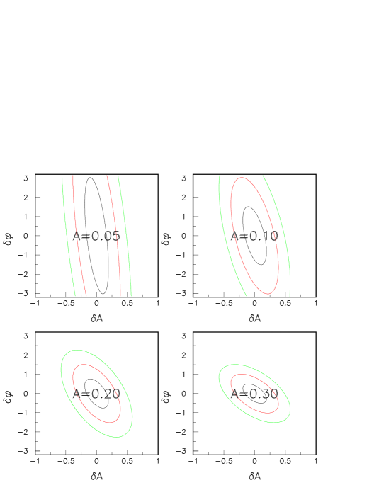
Figure 3: Contours of equal probability in the $\delta A-\delta\phi$ plane

Equation 3.15 is then the expression for the likelihood for this set of events. The inverse of the covariance matrix for the variables $A$ and $\phi$, $G=V^{-1}$, is given by

$$G_{AA}=-\frac{\partial^{2}\ln{\cal L}}{\partial A^{2}}\ \ \ \ G_{\phi\phi}=-\frac{\partial^{2}\ln{\cal L}}{\partial\phi^{2}}\ \ \ \ G_{A\phi}=-\frac{\partial^{2}\ln{\cal L}}{\partial A\partial\phi}$$ (3.16)

The covariance matrix is computed in appendix A.

The one sigma contour in the $A-\phi$ plane is given by the ellipse equation:

$$\frac{1}{1-\rho^{2}}\left[\frac{\delta A^{2}}{\sigma^{2}_{A}}-\frac{2\rho\delta A\delta\phi}{\sigma_{A}\sigma_{\phi}}+\frac{\delta\phi^{2}}{\sigma^{2}_{\phi}}\right]=1$$ (3.17)

where $\delta A=A-{\bar{A}}$, $\delta\phi=\phi-{\bar{\phi}}$ and ${\bar{A}}$, ${\bar{\phi}}$ are the “true” values, and $\rho$ is the correlation coefficient. This error ellipse is shown in figure 3 for four different values of the asymmetry $A$, and $\phi=0.1$. It can be seen that the error on $\phi$ decreases as the asymmetry gets larger.

4 Extraction of $\alpha$ given $A$, $\phi$, and $B_{avg}$

As discussed in Section 2, there are three observables related to the CP asymmetry in $B\rightarrow\pi\pi$. The uncertainties on the measurements of $A$ and $\phi$ were discussed in Section 3. The third observable, $B_{avg}$, can be measured from untagged events, and will therefore have a very low statistical error. The extent to which systematic uncertainties can be controlled will therefore be a crucial consideration. While absolute branching ratios are very difficult to obtain, it will be sufficient to measure the branching ratio relative to the process $B^{0}\to\ell^{+}\pi^{-}\nu$.

There are five unknowns that influence the values of the 3 observables:

• $\alpha$, the weak phase we are trying to extract from these measurements.

• $A_{T}$, the amplitude of the tree diagram. Assuming factorization, the amplitudes for $B^{0}\to\ell^{+}\pi^{-}\nu$ and $B^{0}\to\pi^{-}\pi^{+}$ are proportional to a common form-factor, spanning a range of $q^{2}$ for the first case, and evaluated at $q^{2}=m_{\pi}^{2}$ for the latter case[10]. Ref. [11] points out that color-allowed $B$ decays are well described by factorized amplitudes, but find that it is necessary to add non-factorized amplitudes to describe color-suppressed $B$ decays. Since the decay $B^{0}\to\pi^{-}\pi^{+}$ is color allowed, we assume that the decay $B^{0}\to\ell^{+}\pi^{-}\nu$ will be observed in conjunction with $B^{0}\to\pi^{-}\pi^{+}$ and used to predict $A_{T}$.

• $A_{P}$, the amplitude of the penguin diagram. This amplitude can be estimated from measurements of the decay $B^{0}\to K^{-}\pi^{+}$, applying SU(3) corrections, and scaling by $|V_{td}/V_{ts}|$[7]. Some complications are that this decay may in turn have a contribution from tree diagrams, and furthermore, there may be electroweak contributions that invalidate the SU(3) correspondence[8]. The decay mode $B_{s}\to\phi\rho^{0}$ may possibly be used to check our understanding of these effects[12]. We assume that the relative size of the signals for $B^{0}\to K^{-}\pi^{+}$ and $B^{0}\to\pi^{-}\pi^{+}$ will determine $A_{P}$, although with less precision than for $A_{T}$.

• The weak phase of the penguin amplitude. The top quark dominates in the loop, therefore this phase will be $-\beta$ to a good approximation[13]. As shown in equation 2.13, in this case we are not sensitive to the value of $\beta$.

• The strong phase difference, $\delta$, between the tree and penguin diagrams. There is a perturbative phase difference of order $10^{\circ}$[8], and there are also nonperturbative effects from hadronization that are expected to be small but are incalculable. The phase shift between the I=0 and I=2 amplitudes can be obtained from a measurement of the branching ratios of $B\to\pi^{+}\pi^{-}$, $B\to\pi^{+}\pi^{0}$, and $B\to\pi^{0}\pi^{0}$. This check can be done at a symmetric $e^{+}e^{-}$ collider, and does not require flavor tagging or time-ordering. The question then becomes: Is there a difference in the hadronization for a penguin diagram and I=0 tree diagram? The extent to which these phase shifts can be constrained helps constrain our solution for $\alpha$.

Given an assumption for the central values of these parameters, we can calculate the values of $A$, $\phi$, and $B_{avg}$. Given an assumption for the effective number of tagged events, $N_{tag}$[15], we can calculate the error matrix for $A$ and $\phi$. We will make assumptions on the uncertainties on $A_{T}$, $A_{P}$, $\delta$, and $B_{avg}$, parametrized as Gaussians with widths $\sigma(A_{T})$, $\sigma(A_{P})$, $\sigma(\delta)$, and $\sigma(B_{avg})$. With these assumptions, we can form a $\chi^{2}$. The minimization program MINUIT is used to minimize this $\chi^{2}$, return the input value of $\alpha$, and estimate the expected uncertainty on a measurement of $\alpha$.

Figure 4: One $\sigma$ errors on $\alpha$ as a function of the input value of $\alpha$. The solid line shows the positive errors, and the dashed line the negative errors: (a) $A_{P}=0$, and fixed to 0 in the fits. The following assume $A_{P}=0.2$: (b) $\sigma(A_{P})/A_{P}=0.1$, $\sigma(A_{T})/A_{T}=0.03$, $\sigma(\delta)=20^{\circ}$, and $\sigma(B_{avg})/B_{avg}=0.06.$ (c) $A_{P}$, $A_{T}$, and $\delta$ held fixed in the fits, and $\sigma(B_{avg})/B_{avg}=0.06.$ (d) $\sigma(A_{P})/A_{P}=0.1$, $\sigma(A_{T})/A_{T}=0.015$, $\sigma(\delta)=20^{\circ}$, and $\sigma(B_{avg})/B_{avg}=0.03.$

Unless specfied otherwise, we use the following as default values of the parameters:

• $N_{tag}=100$, starting at $c\tau$ = 1.6 lifetimes[16].

• $A_{T}=1.0$

• $A_{P}=0.2$

• $\delta=0.0$

Figure 5: $N\sigma$ as a function of $\alpha$, for an input value of $\alpha=47^{\circ}$ on the left and $\alpha=67^{\circ}$ on the right. The input value for $A_{P}/A_{T}$ is 0.05. For the following, we assume $\sigma(B_{avg})/B_{avg}=0.06$: (a) $\sigma(A_{P})/A_{P}=1.0$, $\sigma(A_{T})/A_{T}=1.0$, no constraint on $\delta$. (b) $\sigma(A_{P})/A_{P}=1.0$, $\sigma(A_{T})/A_{T}=0.03$, no constraint on $\delta$. (c) $\sigma(A_{P})/A_{P}=1.0$, $\sigma(A_{T})/A_{T}=0.03$, $\sigma(\delta)=20^{\circ}$. (d) $\sigma(A_{P})/A_{P}=0.1$, $\sigma(A_{T})/A_{T}=0.03$, no constraint on $\delta$. (e) $\sigma(A_{P})/A_{P}=0.1$, $\sigma(A_{T})/A_{T}=0.03$, $\sigma(\delta)=20^{\circ}$.

In Fig. 4 we show the expected $1\sigma$ errors as a function of $\alpha$ for various conditions. In Fig. 4a, we show the errors for the case where $A_{P}=0.0$, and has been constrained to zero in the fit. We see that the errors are largest for $\alpha$ near $45^{\circ}$ and $135^{\circ}$, where the dependence of $\sin(2\alpha)$ on $\alpha$ is lowest. In Fig. 4b, c, and d, we show the errors for the case where $A_{P}=0.2$ and we are able to put the specified constraints on the amplitudes. We see that in the case where there is a penguin amplitude, and it is well understood, in general, the errors are smaller than in the case of no penguin amplitude.

Figure 6: $N\sigma$ as a function of $\alpha$, for an input value of $\alpha=47^{\circ}$ on the left and $\alpha=67^{\circ}$ on the right. The input value for $A_{P}/A_{T}$ is 0.2. For the following, we assume $\sigma(B_{avg})/B_{avg}=0.06$: (a) $\sigma(A_{P})/A_{P}=1.0$, $\sigma(A_{T})/A_{T}=1.0$, no constraint on $\delta$. (b) $\sigma(A_{P})/A_{P}=1.0$, $\sigma(A_{T})/A_{T}=0.03$, no constraint on $\delta$. (c) $\sigma(A_{P})/A_{P}=1.0$, $\sigma(A_{T})/A_{T}=0.03$, $\sigma(\delta)=20^{\circ}$. (d) $\sigma(A_{P})/A_{P}=0.1$, $\sigma(A_{T})/A_{T}=0.03$, no constraint on $\delta$. (e) $\sigma(A_{P})/A_{P}=0.1$, $\sigma(A_{T})/A_{T}=0.03$, $\sigma(\delta)=20^{\circ}$. For the following, we assume $\sigma(B_{avg})/B_{avg}=0.03$: (f) $\sigma(A_{P})/A_{P}=0.1$, $\sigma(A_{T})/A_{T}=0.015$, $\sigma(\delta)=20^{\circ}$

The plots in Fig. 4 do not convey all the relevant information on the constraints on $\alpha$. The errors are highly non-Gaussian, and there are multiple minima. To gain further insight, we choose two particular input values for $\alpha$, $47^{\circ}$ and $67^{\circ}$. We then scan as a function of the assumed value of $\alpha$ in the fit. For each point in the scan, we hold $\alpha$ fixed, and mimimize the $\chi^{2}$ with respect to all the other parameters. We then plot $\sqrt{\chi^{2}-\chi^{2}_{min}}$ as a function of $\alpha$, interpreting $\sqrt{\chi^{2}-\chi^{2}_{min}}$ as the number of standard deviations on $\alpha$.

We show the results in Fig. 5 for the case $A_{P}/A_{T}=0.05$. In Fig. 5a, we assume very little knowledge of the tree and penguin parameters. We see that when the penguin contribution is small, loose constraints are sufficient for the determination of $\alpha$. However, even with the tight constraints of Fig. 5e we are unable to lift the discrete ambiguities.

We show the results in Fig. 6 for the case $A_{P}/A_{T}=0.2$. In Fig. 6a, we assume very little knowledge of the tree and penguin parameters. As qualitatively pointed out in Ref [14], in this case, we can rule out only a small fraction of the available parameter space. As we add constraints in Fig. 6b, c, and d, there are fewer minima and more of the parameter space can be ruled out. As shown in Fig. 6e, it is not until we constrain all the parameters that we are left with a single minimum. Tightening the constraints in Fig. 6f, we more convincingly rule out alternative minima and improve the precision of the measurement of $\alpha$.

In Fig. 7, we show similar plots as for Fig. 6, using the same input values for $\alpha$ but negative assumed values for $\alpha$. As discussed earlier, there is another solution only for the discrete case $A=0$. However, even for other values of $A$, two solutions may be allowed within the uncertainties of the measurement. Fig. 7 illustrates how well we can choose between the solutions. The separation is quite convincing for $\alpha=47^{\circ}$, i.e. for large values of $A$, and becomes more difficult for $\alpha=67^{\circ}$, i.e. as $A$ gets smaller.

Figure 7: $N\sigma$ as a function of $-\alpha$, for an input value of $\alpha=47^{\circ}$ on the left and $\alpha=67^{\circ}$ on the right. For the following, we assume $\sigma(B_{avg})/B_{avg}=0.06$: (a) $\sigma(A_{P})/A_{P}=0.1$, $\sigma(A_{T})/A_{T}=0.03$, $\sigma(\delta)=20^{\circ}$. For the following, we assume $\sigma(B_{avg})/B_{avg}=0.03$: (b)$\sigma(A_{P})/A_{P}=0.1$, $\sigma(A_{T})/A_{T}=0.015$, $\sigma(\delta)=20^{\circ}$.

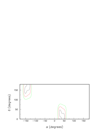
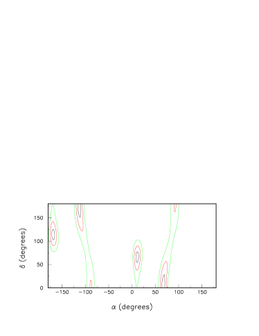
Figure 8: One, two, and three $\sigma$ contours as a function of $\alpha$ and $\delta$, for input values of $\alpha=47^{\circ}$, $\delta=0^{\circ}$, and $A_{P}/A_{T}$ = 0.2.

Figure 9: One, two, and three $\sigma$ contours as a function of $\alpha$ and $\delta$, for input values of $\alpha=67^{\circ}$, $\delta=0^{\circ}$, and $A_{P}/A_{T}$ = 0.2.

It is clear from the above plots that knowledge of the strong phase difference $\delta$ decreases the error on $\alpha$ and in addition can help distinguish between the discrete solutions on $\alpha$. Figures 9 and 9 are similar to Figure 6, except we scan as a function of assumed values for both $\alpha$ and $\delta$, and plot constant contours in $\sqrt{\chi^{2}-\chi^{2}_{min}}$. In the case of $\alpha=47^{\circ}$ there are only two minima, and one needs to know $\delta$ to better than $60^{\circ}$ in order to distinguish between the two discrete solutions by $2\sigma$. In the more complicated case of $\alpha=67^{\circ}$, there are multiple solutions even within the first two quadrants for $\alpha$. Here a more precise knowledge of $\delta$ is required to unambiguously extract $\alpha$.

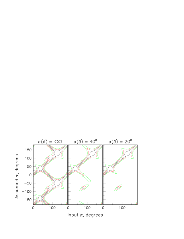
Figure 10: One, two, and three $\sigma$ contours as a function of input value of $\alpha$ and assumed value of $\alpha$, for various values of $\sigma_{\delta}$. Note that there always remains a discrete ambiguity between $\alpha$ and $-\alpha$ where $A=0$.

The above two values of $\alpha$ of $47^{\circ}$ and $67^{\circ}$ lead to quite different conclusions on the knowledge of $\delta$ required for a unique determination of $\alpha$. We have also investigated the effect of the uncertainty on $\delta$ on the extraction of $\alpha$, for all values of $\alpha$. As an example, Figure 10 shows constant contours of $\sqrt{\chi^{2}-\chi^{2}_{min}}$ in the plane of input value of $\alpha$ and assumed value of $\alpha$, for three different constraints on $\delta$. We see that the discrimination between discrete ambiguities improves with the precision on $\delta$ until the uncertainty on $\delta$ reaches a value of $20^{\circ}$. We find that this result holds for all values of $\alpha$.

5 Conclusions

We have presented the results of an error analysis on $\alpha$, given a measurement of the time-dependent asymmetry between $B^{0}\to\pi^{+}\pi^{-}$ and ${\bar{B}^{0}}\to\pi^{+}\pi^{-}$, a measurement of the average branching ratio for $B$ and $\bar{B}$ decays to $\pi^{+}\pi^{-}$, and constraints on the magnitudes $A_{T}$ and $A_{P}$ and relative phase $\delta$ of the tree and penguin diagrams. While there are an infinite number of possible scenarios, our results set the scale for how well these parameters need to be known. We have considered scenarios in which we have an effective number of 100 perfectly tagged signal events[15].

In the case where the penguin contribution is small ($A_{P}/A_{T}\approx 0.05$), only crude information on $A_{P}$ and $A_{T}$ is needed for the extraction of $\alpha$. However, we are left with four discrete ambiguities, as in the case where there is no penguin contribution.

In the case where the penguin contribution is larger ($A_{P}/A_{T}\approx 0.2$), more precise information on $A_{P}$ and $A_{T}$ is needed. If this precision can be achieved, the uncertainty on $\alpha$ is in many cases smaller than for the case of no penguin amplitude. Furthermore, if it is possible to place constraints on $\delta$, some or all of the discrete ambiguities may be lifted. A large penguin amplitude therefore presents an opportunity for a much improved determination of $\alpha$.

In summary, we find that if the penguin amplitudes are either small or well understood then it is possible to determine $\alpha$ from the CP asymmetry in $B^{0}\to\pi^{+}\pi^{-}$ without resorting to the observation of final states with neutral particles. Thus, measurements would be feasible at hadron colliders as well as $e^{+}e^{-}$ colliders. Furthermore, a large penguin amplitude presents an opportunity for improved precision on $\alpha$ while lifting some or all of the discrete ambiguities.

6 Acknowledgements

This study was performed in the context of discussions on the physics goals and detector upgrades for CDF in Run 2. We thank our collaborators for their kind advice and comments. In addition, we thank Isi Dunietz, Chris Hill, Jonathan Lewis, and Jon Rosner for useful discussions.

Appendix A Likelihood formalism for the extraction of fitting errors

The analysis follows closely that in reference [17]. For brevity, we define the functions $n_{\pm}(t)$:

$$n_{\pm}(A,\phi,t)=1\pm A\sin(xt+\phi)$$ (A.1)

With this notation, and ignoring an irrelevant constant term, the log-likelihood (see equation 3.15) is

$$\ln{\cal L}(A,\phi)=\sum_{i}\ln n_{+}(A,\phi,t_{i})+\sum_{j}\ln n_{-}(A,\phi,t_{j})$$ (A.2)

The second derivatives of the above function are the elements of the inverse of the correlation matrix, $G=V^{-1}$. For example,

$$G_{AA}=-\frac{\partial^{2}\ln{\cal L}}{\partial A^{2}}={\sum_{i}\frac{\sin^{2}(xt_{i}+\phi)}{[n_{+}(t_{i})]^{2}}}+{\sum_{j}\frac{\sin^{2}(xt_{j}+\phi)}{[n_{-}(t_{j})]^{2}}}$$ (A.3)

These sums can be approximated by integrals:

$$\sum_{k}f_{\pm}(t_{k})\approx\int_{T}^{\infty}f_{\pm}(t)N_{\pm}(t)dt$$ (A.4)

where the limits of integration assume that a lifetime cut is imposed on the reconstructed mesons, and $N_{\pm}(t)$ are defined in equation 3.14. Since in general $f_{\pm}(t)=g_{\pm}(t)/[n_{\pm}(t_{i})]^{2}$, equation A.3 (for the general error on variables $p$ and $q$) thus becomes

$$G_{pq} = \frac{N}{2}{\int_{T}^{\infty}e^{-t}\left[\frac{g_{+}(t)}{n_{+}(t)}+\frac{g_{-}(t)}{n_{-}(t)}\right]dt}$$ (A.5)

$$= \frac{N}{2}{\int_{T}^{\infty}e^{-t}\left[g_{+}(t)n_{-}(t)+g_{-}(t)n_{+}(t)\right]dt}$$ (A.6)

where we have ignored terms which of order $A^{2}$:

$$n_{+}(t)n_{-}(t)=1-A^{2}\sin^{2}(xt+\phi)\approx 1.$$ (A.7)

We expect this to be a reasonable approximation even for extreme values of $\sin(2\alpha)$, since in practice the observed asymmetry will be reduced by a dilution factor $D\sim 0.5$ resulting from imperfect flavor tagging. With some algebra, we obtain

$$G_{AA} = N{\int_{T}^{\infty}e^{-t}\sin^{2}(xt+\phi)dt}$$ (A.8)

$$G_{\phi\phi} = NA^{2}{\int_{T}^{\infty}e^{-t}\cos^{2}(xt+\phi)dt}$$ (A.9)

$$G_{A\phi} = \frac{N}{2}A{\int_{T}^{\infty}e^{-t}\sin 2(xt+\phi)dt}$$ (A.10)

We note that, as expected, these equations are invariant with respect to the following transformation in the presence of dilutions:

$$A \rightarrow DA$$ (A.11)

$$N \rightarrow \frac{N}{D^{2}}$$ (A.12)

For brevity, we introduce two new functions, $P_{c}(x,T)$ and $P_{s}(x,T)$ given by

$$P_{c}(x,T)=\frac{1}{1+x^{2}}\left[\cos xT-x\sin xT\right]$$ (A.13)

$$P_{s}(x,T)=\frac{1}{1+x^{2}}\left[x\cos xT+\sin xT\right]$$ (A.14)

and the end result is

$$G_{AA} = \frac{N}{2}e^{-T}\left[1-P_{c}(2x,t_{o})\right]$$ (A.15)

$$G_{\phi\phi} = A^{2}\frac{N}{2}e^{-T}\left[1+P_{c}(2x,t_{o})\right]$$ (A.16)

$$G_{A\phi} = \frac{N}{2}e^{-T}AP_{s}(2x,t_{o})$$ (A.17)

where $t_{o}=T+{\phi\over x}$.

References

[1] For a review see: B Decays, edited
by S. Stone, World Scientific, 1994.
[2] I.I. Bigi and A.I. Sanda, Nucl. Phys. B193 85, (1981;)B281, 41 (1987); I. Dunietz in ref [1];
Y. Nir and H. Quinn in ref [1].
[3] M. Gronau and D. London, Phys. Rev. Letters 65 3381, (1990.)
[4] R. Aleksan, I. Dunietz and B. Kayser, Zeit. Phys. C54 653, (1992.)
[5] M. Gronau and D. Wyler, Phys. Lett. B265 172, (1991.)
[6] R. Aleksan, A. Gaidot, and G. Vaisseur,
DAPNIA/SPP 92-19.
[7] J.P. Silva and L. Wolfenstein, Phys. Rev. D49 1151, (1994.)
[9] M. Gronau, Phys. Rev. Letters 63 1451, (1989.)
[10] M. Bauer, B. Stech, M. Wirbel, Zeit. Phys. C34 103, (1987;)M. Wirbel, B. Stech, M. Bauer, Zeit. Phys. C29 637, (1985.)
[11] A.N. Kamal and A.B. Santra, ALBERTA-THY-31-94, Oct 1994.
[12] N.G. Deshpande, X.G. He, J. Trampetic, Phys. Lett. B345 547, (1995.)
[13] A. Deandrea, N. Di Bartolomeo, R. Gatto, F. Feruglio,
and N. Nardulli, Phys. Lett. B320 170, (1994;)D. London and R.D. Peccei, Phys. Lett. B223 257, (1989.)
[14] M. Gronau, Phys. Lett. B300 163, (1993.)
[15] For a sample of signal events, on
top of a background of events, the uncertainty on
the CP asymmetry, , is given by
where is
the efficiency of the flavor-tagging algorithm and is
the “dilution” of the algorithm, defined as
where are the number
of correct and incorrect tags respectively. The effective number
of tagged signal events is thus .
[16] J.D. Lewis, J. Mueller, J. Spalding, and P. Wilson,
Proceedings of the Workshop on B physics at Hadron Accelerators, p. 217,
Snowmass, Colorado, June 21 - July 2, 1993. Editors: P. McBride and
C.S. Shukla.
[17] K. McDonald, “Maximum Likelihood Analysis for CP-Violating
Asymmetries”, Princeton Preprint, Princeton/HEP/92-04.