EPS-HEP 95 Ref. eps0631 IEKP-KA/95-07
hep-ph/9507291

Combined Fit of Low Energy Constraints to
Minimal Supersymmetry and Discovery Potential at LEP II
W. de Boer, G. Burkart, R. Ehret, W. Oberschulte-Beckmann
Inst. für Experimentelle Kernphysik, Univ. of Karlsruhe
Postfach 6980, D-76128 Karlsruhe 1, FRG
and

V. Bednyakov, S.G. Kovalenko
Bogoliubov Lab. of Theor. Physics, Joint Inst. for Nucl. Research,
141 980 Dubna, Moscow Region, RUSSIA

Abstract

Within the Constrained Minimal Supersymmetric Standard Model (CMSSM) it is possible to predict the low energy gauge couplings and masses of the 3. generation particles from a few parameters at the GUT scale. In addition the MSSM predicts electroweak symmetry breaking due to large radiative corrections from Yukawa couplings, thus relating the $Z^{0}$ boson mass to the top quark mass.

From a $\chi^{2}$ analysis, in which these constraints are considered simultaneously, one can calculate the probability for each point in the MSGUT parameter space. The recently measured top quark mass prefers two solutions for the mixing angle in the Higgs sector: $\tan\beta$ in the range between 1 and 3 or alternatively $\tan\beta\approx 15-50$. For both cases we find a unique $\chi^{2}$ minimum in the parameter space. From the corresponding most probable parameters at the GUT scale, the masses of all predicted particles can be calculated at low energies using the RGE, albeit with rather large errors due to the logarithmic nature of the running of the masses and coupling constants. Our fits include full second order corrections for the gauge and Yukawa couplings, low energy threshold effects, contributions of all (s)particles to the Higgs potential and corrections to $m_{b}$ from gluinos and higgsinos, which exclude (in our notation) positive values of the mixing parameter in the Higgs potential $\mu$ for the large $\tan\beta$ region.

Further constraints can be derived from  the branching ratio for the radiative (penguin) decay of the b-quark into $s\gamma$ and the lower limit on the lifetime of the universe, which requires the dark matter density due to the Lightest Supersymmetric Particle (LSP) not to overclose the universe.

For the low $\tan\beta$ solution these additional constraints can be fulfilled simultaneously for quite a large region of the parameter space. In contrast, for the high $\tan\beta$ solution the correct value for the $b\rightarrow s\gamma$ rate is obtained only for small values of the gaugino scale and electroweak symmetry breaking is difficult, unless one assumes the minimal SU(5) to be a subgroup of a larger symmetry group, which is broken between the Planck scale and the unification scale. In this case small splittings in the Yukawa couplings are expected at the unification scale and electroweak symmetry breaking is easily obtained, provided the Yukawa coupling for the top quark is slightly above the one for the bottom quark, as expected e.g. if the larger symmetry group would be SO(10).

For particles, which are most likely to have masses in the LEP II energy range, the cross sections are given for the various energy scenarios at LEP II. The highest LEP II energies (205 GeV) are just high enough to cover a large region of the preferred parameter space, both for the low and high ${\tan\beta}$ solutions. For low ${\tan\beta}$ the production of the lightest Higgs boson, which is expected to have a mass below 115 GeV, is the most promising channel, while for large ${\tan\beta}$ the production of Higgses, charginos and/or neutralinos covers the preferred parameter space.

1 Introduction

Grand Unified Theories (GUT’s) in which the electroweak and strong forces are unified at a scale $M_{\rm GUT}$ of the order $10^{16}$ GeV are strongly constrained by low energy data, if one imposes unification of gauge- and Yukawa couplings as well as electroweak symmetrybreaking. The Minimal Supersymmetric Standard Model (MSSM) [1] has become the leading candidate for a GUT after the precisely measured coupling constants at LEP excluded unification in the Standard Model [2, 3, 4]. In the MSSM the quadratic divergences in the higher order radiative corrections largely cancel, so one can calculate the corrections reliably even over many orders of magnitude. The large hierarchy between the electroweak scale and the unification scale as well as the different strengths of the forces at low energy are naturally explained by the radiative corrections[5]. Low energy data on masses and couplings provide strong constraints on the MSSM parameter space, as discussed recently by many groups  [6, 7, 8, 9, 10, 11, 12, 13, 14, 15, 16, 17, 18, 19, 20].

In this paper we perform a combined statistical analysis of the low energy constraints, namely the three gauge coupling constants measured at LEP, the quark- and leptonmasses of the third generation, the lower limit on the as yet unobserved supersymmetric particles, the $Z^{0}$-boson mass, the radiative decay $b\rightarrow s\gamma$ observed by CLEO [21], and the lower limit on the lifetime of the universe, which requires the dark matter density from the Lightest Supersymmetric Particle (LSP) not to overclose the universe. No restriction is made on $\tan\beta$ , the ratio of vacuum expectation values of the neutral components of the Higgsfields. Therefore both the low $\tan\beta$ solution, expected in the SU(5), and the high $\tan\beta$ solution, expected in SO(10), are considered.

The theoretically more questionable constraint from proton decay in the MSSM [22, 23], which involve the unknown Higgs sector at the GUT scale, was considered in a similar analysis before[14]. At large ${\tan\beta}$ values one needs a different multiplet structure[24] or a larger Higgs sector[25].

Assuming soft symmetry breaking at the GUT-scale, all SUSY masses can be expressed in terms of 5 parameters and the masses at low energy are then determined by the well known Renormalization Group Equations (RGE). The experimental constraints are sufficient to determine these parameters, albeit with large uncertainties. From the statistical analysis we obtain the probability for every point in the SUSY parameter space, which allows us to calculate the cross sections for the expected new physics of the MSSM at LEP II. These cross sections will be given as function of the common scalar and gaugino masses at the GUT-scale, denoted by $m_{0}$ , $m_{1/2}$ ; for each choice of $m_{0}$ , $m_{1/2}$ , the other parameters were determined from the constraint fit.

2 The Model

2.1 The Lagrangian

The minimal supersymmetric extension of the Standard Model is described by the Lagrangian containing the SUSY-symmetric part together with SUSY breaking terms originating from supergravity [26]. The breaking terms of the Lagrangian are given by:

$${\cal L}_{Breaking} = -m_{0}^{2}\sum_{i}|\varphi_{i}|^{2}-m_{1/2}\sum_{j}\lambda_{j}\lambda_{j}$$

$$- Am_{0}\left[h_{u}^{ab}Q_{a}U^{c}_{b}H_{2}+h_{d}^{ab}Q_{a}D^{c}_{b}H_{1}+h_{e}^{ab}L_{a}E^{c}_{b}H_{1}\right]-Bm_{0}\left[\mu H_{1}H_{2}\right].$$

The Lagrangian given above assumes that squarks and sleptons have a common mass $m_{0}$ and the gauginos a common mass $m_{1/2}$ at the GUT scale. The SUSY Lagrangian contains the following free parameters:

• 3 gauge couplings $\alpha_{i}$,

• the Yukawa couplings $h_{i}^{ab}$, where $i$ is the flavour index and $ab$ are generation indices. Since the masses of the third generation are much larger than masses of the first two ones, we consider only the Yukawa coupling of the third geneeration and drop the indices $a,b$.

• the Higgs field mixing parameter $\mu$.

They are supplemented by the soft breaking ones:

• $m_{0},\ m_{1/2},\ A,\ B$, where A and B are the coupling constants for the Higgs fields.

With these parameters the comlete mass spectrum of the SUSY particles is determined.

2.2 The SUSY Mass Spectrum

All couplings and masses become scale dependent due to radiative corrections. This running is described by the renormalization group equations (RGE) [8]:

3 Couplings: ($i=1,2,3$)

$$\frac{d{\tilde{\alpha}}_{i}}{dt} = -b_{i}{\tilde{\alpha}}_{i}^{2}-{\tilde{\alpha}}_{i}^{2}\left(\sum_{j=1}^{3}b_{ij}{\tilde{\alpha}}_{j}-\sum_{U,D,L}a_{ij}Y_{j}\right)$$ (2)

$$\frac{dY_{U}}{dt} = Y_{U}\sum_{i=1}^{6}\left(c^{t}_{i}{\tilde{\alpha}}_{i}-\sum_{j\geq i}^{6}c^{t}_{ij}{\tilde{\alpha}}_{i}{\tilde{\alpha}}_{j}\right)$$ (3)

$$\frac{dY_{D}}{dt} = Y_{D}\sum_{i=1}^{6}\left(c^{b}_{i}{\tilde{\alpha}}_{i}-\sum_{j\geq i}^{6}c^{b}_{ij}{\tilde{\alpha}}_{i}{\tilde{\alpha}}_{j}\right)$$ (4)

$$\frac{dY_{L}}{dt} = Y_{L}\sum_{i=1}^{6}\left(c^{\tau}_{i}{\tilde{\alpha}}_{i}-\sum_{j\geq i}^{6}c^{\tau}_{ij}{\tilde{\alpha}}_{i}{\tilde{\alpha}}_{j}\right)$$ (5)

3 Gauginos: ($i=1,2,3$)

$$\frac{dM_{i}}{dt} = -b_{i}\tilde{\alpha}_{i}^{2}M_{i}$$ (6)

Masses of the 1st. and 2nd Generation ($i=1,2$):

$$\frac{d\tilde{m}^{2}_{L_{i}}}{dt} = 3(\tilde{\alpha}_{2}M^{2}_{2}+\frac{1}{5}\tilde{\alpha}_{1}M^{2}_{1})$$ (7)

$$\frac{d\tilde{m}^{2}_{E_{i}}}{dt} = (\frac{12}{5}\tilde{\alpha}_{1}M^{2}_{1})$$ (8)

$$\frac{d\tilde{m}^{2}_{Q_{i}}}{dt} = (\frac{16}{3}\tilde{\alpha}_{3}M^{2}_{3}+3\tilde{\alpha}_{2}M^{2}_{2}+\frac{1}{15}\tilde{\alpha}_{1}M^{2}_{1})$$ (9)

$$\frac{d\tilde{m}^{2}_{U_{i}}}{dt} = (\frac{16}{3}\tilde{\alpha}_{3}M^{2}_{3}+\frac{16}{15}\tilde{\alpha}_{1}M^{2}_{1})$$ (10)

$$\frac{d\tilde{m}^{2}_{D_{i}}}{dt} = (\frac{16}{3}\tilde{\alpha}_{3}M^{2}_{3}+\frac{4}{15}\tilde{\alpha}_{1}M^{2}_{1})$$ (11)

Masses of the 3th Generation ($i=3$):

$$\frac{d\tilde{m}^{2}_{L_{i}}}{dt} = 3(\tilde{\alpha}_{2}M^{2}_{2}+\frac{1}{5}\tilde{\alpha}_{1}M^{2}_{1})-Y_{L}(\tilde{m}^{2}_{L}+\tilde{m}^{2}_{E}+m^{2}_{H_{D}}+A^{2}_{L}m_{0}^{2})$$ (12)

$$\frac{d\tilde{m}^{2}_{E_{i}}}{dt} = (\frac{12}{5}\tilde{\alpha}_{1}M^{2}_{1})-2Y_{L}(\tilde{m}^{2}_{L}+\tilde{m}^{2}_{E}+m^{2}_{H_{D}}+A^{2}_{L}m_{0}^{2})$$ (13)

$$\frac{d\tilde{m}^{2}_{Q_{i}}}{dt} = (\frac{16}{3}\tilde{\alpha}_{3}M^{2}_{3}+3\tilde{\alpha}_{2}M^{2}_{2}+\frac{1}{15}\tilde{\alpha}_{1}M^{2}_{1})-$$

$$\left[Y_{U}(\tilde{m}^{2}_{Q}+\tilde{m}^{2}_{U}+m^{2}_{H_{U}}+A^{2}_{U}m_{0}^{2})+Y_{D}(\tilde{m}^{2}_{Q}+\tilde{m}^{2}_{D}+m^{2}_{H_{D}}+A^{2}_{D}m_{0}^{2})\right],$$

$$\frac{d\tilde{m}^{2}_{U_{i}}}{dt} = (\frac{16}{3}\tilde{\alpha}_{3}M^{2}_{3}+\frac{16}{15}\tilde{\alpha}_{1}M^{2}_{1})-2Y_{U}(\tilde{m}^{2}_{Q}+\tilde{m}^{2}_{U}+m^{2}_{H_{U}}+A^{2}_{U}m_{0}^{2}),$$ (15)

$$\frac{d\tilde{m}^{2}_{D_{i}}}{dt} = (\frac{16}{3}\tilde{\alpha}_{3}M^{2}_{3}+\frac{4}{15}\tilde{\alpha}_{1}M^{2}_{1})-2Y_{D}(\tilde{m}^{2}_{Q}+\tilde{m}^{2}_{D}+m^{2}_{H_{D}}+A^{2}_{D}m_{0}^{2})$$ (16)

Higgs potential parameters:

$$\frac{d\mu^{2}}{dt} = \mu^{2}\left[3(\tilde{\alpha}_{2}+\frac{1}{5}\tilde{\alpha}_{1})-(3Y_{U}+3Y_{D}+Y_{L})\right]$$ (17)

$$\frac{dm^{2}_{1}}{dt} = 3(\tilde{\alpha}_{2}M^{2}_{2}+\frac{1}{5}\tilde{\alpha}_{1}M^{2}_{1})+3(\tilde{\alpha}_{2}+\frac{1}{5}\tilde{\alpha}_{1})\mu^{2}-(3Y_{U}+3Y_{D}+Y_{L})\mu^{2}$$ (19)

$$-3Y_{D}(\tilde{m}^{2}_{Q}+\tilde{m}^{2}_{D}+m^{2}_{1}-\mu^{2}+A^{2}_{D}m_{0}^{2})-Y_{E}(\tilde{m}^{2}_{L}+\tilde{m}^{2}_{E}+m^{2}_{1}-\mu^{2}+A^{2}_{L}m_{0}^{2})$$

$$\frac{dm^{2}_{2}}{dt} = 3(\tilde{\alpha}_{2}M^{2}_{2}+\frac{1}{5}\tilde{\alpha}_{1}M^{2}_{1})+3(\tilde{\alpha}_{2}+\frac{1}{5}\tilde{\alpha}_{1})\mu^{2}-(3Y_{U}+3Y_{D}+Y_{E})\mu^{2}$$ (21)

$$-3Y_{U}(\tilde{m}^{2}_{Q}+\tilde{m}^{2}_{U}+m^{2}_{2}-\mu^{2}+A^{2}_{U}m_{0}^{2})$$

Trilinear couplings:

$$\frac{dA_{U}}{dt} = -\left(\frac{16}{3}\tilde{\alpha}_{3}\frac{M_{3}}{m_{0}}+3\tilde{\alpha}_{2}\frac{M_{2}}{m_{0}}+\frac{13}{15}\tilde{\alpha}_{1}\frac{M_{1}}{m_{0}}\right)-6Y_{U}A_{U}-Y_{D}A_{D}$$ (23)

$$\frac{dA_{D}}{dt} = -\left(\frac{16}{3}\tilde{\alpha}_{3}\frac{M_{3}}{m_{0}}+3\tilde{\alpha}_{2}\frac{M_{2}}{m_{0}}+\frac{7}{15}\tilde{\alpha}_{1}\frac{M_{1}}{m_{0}}\right)-6Y_{D}A_{D}-Y_{U}A_{U}-Y_{L}A_{L}$$ (24)

$$\frac{dA_{L}}{dt} = -\left(3\tilde{\alpha}_{2}\frac{M_{2}}{m_{0}}+\frac{9}{5}\tilde{\alpha}_{1}\frac{M_{1}}{m_{0}}\right)-3Y_{D}A_{D}-4Y_{L}A_{L}$$ (25)

Here $\tilde{m}_{U},\tilde{m}_{D}$ and $\tilde{m}_{E}$ refer to the masses of the superpartners of the quark and lepton singlets, while $\tilde{m}_{Q}$ and $\tilde{m}_{L}$ refer to the masses of the weak isospin doublet superpartners; $m_{1},m_{2},m_{3}$ and $\mu$ are the mass parameters of the Higgs potential (see next section), while $A_{U},A_{D},A_{L}$ and $B$ are the couplings in ${\cal L}_{Breaking}$ as defined before; $M_{i}$ are the gaugino masses before any mixing and the following notation is used:

$${\tilde{\alpha}}_{i}=\frac{\alpha_{i}}{4\pi},\ t=\log(\frac{M_{X}^{2}}{Q^{2}}),Y_{j}=\frac{h_{j}^{2}}{(4\pi)^{2}},$$

where $i=1,2,3$ and $j=U,D,L$. Only the Yukawa couplings of the third generation are considered, so $Y_{U},Y_{D},Y_{L}$ refer to $Y_{t},Y_{b},Y_{\tau}$ and the couplings $h_{j}$ are related to the masses by

$$m_{t} = h_{t}(m_{t})v\sin\beta$$

$$m_{b} = h_{b}(m_{b})v\cos\beta$$

$$m_{\tau} = h_{\tau}(m_{\tau})v\cos\beta$$ (27)

Here $m_{j}$ are the running masses. The boundary conditions at $Q^{2}=M_{\rm GUT}^{2}$ or at $t=0$ are:

$$\tilde{m}^{2}_{Q}=\tilde{m}^{2}_{U}=\tilde{m}^{2}_{D}=\tilde{m}^{2}_{L}=\tilde{m}^{2}_{E}=m_{0}^{2};$$

$$\mu^{2}=\mu_{0}^{2};\ \ \ m_{1}^{2}=m^{2}_{2}=\mu_{0}^{2}+m_{0}^{2};\ \ \$$

$$M_{i}=m_{1/2};\ \ \ {\tilde{\alpha}}_{i}(0)={\tilde{\alpha}}_{\rm GUT},\ \ \ i=1,2,3$$

With given values for $m_{0},m_{1/2},\mu,Y_{t},Y_{b},Y_{\tau},\tan\beta$, and A and correspondingly known boundary conditions at the GUT scale, the differential equations can be solved numerically thus linking the values at the GUT and electroweak scales. The non-negligible Yukawa couplings cause a mixing between the electroweak eigenstates and the mass eigenstates of the third generation particles. The mixing matrices for the $\tilde{m}^{2}_{t},\tilde{m}^{2}_{b}$ and $\tilde{m}^{2}_{\tau}$ are:

$$\left(\begin{array}[]{cc}\tilde{m}_{Q}^{2}+m_{t}^{2}+\frac{1}{6}(4M_{W}^{2}-M_{Z}^{2})\cos 2\beta&m_{t}(A_{t}m_{0}-\mu\cot\beta)\\ m_{t}(A_{t}m_{0}-\mu\cot\beta)&\tilde{m}_{U}^{2}+m_{t}^{2}-\frac{2}{3}(M_{W}^{2}-M_{Z}^{2})\cos 2\beta\end{array}\right)$$

$$\left(\begin{array}[]{cc}\tilde{m}_{Q}^{2}+m_{b}^{2}-\frac{1}{6}(2M_{W}^{2}+M_{Z}^{2})\cos 2\beta&m_{b}(A_{b}m_{0}-\mu\tan\beta)\\ m_{b}(A_{b}m_{0}-\mu\tan\beta)&\tilde{m}_{D}^{2}+m_{b}^{2}+\frac{1}{3}(M_{W}^{2}-M_{Z}^{2})\cos 2\beta\end{array}\right)$$

$$\left(\begin{array}[]{cc}\tilde{m}_{L}^{2}+m_{\tau}^{2}-\frac{1}{2}(2M_{W}^{2}-M_{Z}^{2})\cos 2\beta&m_{\tau}(A_{\tau}m_{0}-\mu\tan\beta)\\ m_{\tau}(A_{\tau}m_{0}-\mu\tan\beta)&\tilde{m}_{E}^{2}+m_{\tau}^{2}+(M_{W}^{2}-M_{Z}^{2})\cos 2\beta\end{array}\right)$$

and the mass eigenstates are the eigenvalues of these mass matrices. The mass matrix for the neutralinos can be written in our notation as:

$${\cal M}^{0}=\left(\begin{array}[]{cccc}M_{1}&0&-M_{Z}\cos\beta\sin_{W}&M_{Z}\sin\beta\sin_{W}\\ 0&M_{2}&M_{Z}\cos\beta\cos_{W}&-M_{Z}\sin\beta\cos_{W}\\ -M_{Z}\cos\beta\sin_{W}&M_{Z}\cos\beta\cos_{W}&0&-\mu\\ M_{Z}\sin\beta\sin_{W}&-M_{Z}\sin\beta\cos_{W}&-\mu&0\end{array}\right)\\$$ (28)

The physical neutralino masses $M_{\tilde{\chi}_{i}^{0}}$ are obtained as eigenvalues of this matrix after diagonalization. The mass matrix for the charginos is:

$${\cal M}^{\pm}=\left(\begin{array}[]{cc}M_{2}&\sqrt{2}M_{W}\sin\beta\\ \sqrt{2}M_{W}\cos\beta&\mu\end{array}\right)$$ (29)

This matrix has two eigenvalues corresponding to the masses of the two charginos  $\tilde{\chi}_{1,2}^{\pm}$:

$$M^{2}_{1,2}=\frac{1}{2}\left[M^{2}_{2}+\mu^{2}+2M^{2}_{W}\mp\sqrt{(M^{2}_{2}-\mu^{2})^{2}+4M^{4}_{W}\cos^{2}2\beta+4M^{2}_{W}(M^{2}_{2}+\mu^{2}+2M_{2}\mu\sin 2\beta)}\right]$$

2.3 Radiative Corrections to the Higgs potential

The Higgs potential $V$ including the one-loop corrections $\quad\Delta V$ can be written as:

$$V(H_{1}^{0},H_{2}^{0}) = m^{2}_{1}|H_{1}^{0}|^{2}+m^{2}_{2}|H_{2}^{0}|^{2}-m^{2}_{3}(H_{1}^{0}H_{2}^{0}+h.c.)+\frac{g^{2}+g^{{}^{\prime}2}}{8}(|H_{1}^{0}|^{2}-|H_{2}^{0}|^{2})^{2}+\quad\Delta V$$

$${\rm with}\quad\Delta V = \frac{1}{64\pi^{2}}\sum_{i}(-1)^{2J_{i}}(2J_{i}+1)C_{i}m_{i}^{4}\left[\ln\frac{m_{i}^{2}}{Q^{2}}-\frac{3}{2}\right],$$ (30)

where the sum is taken over all possible particles. The mass parameters in the potential fulfill the following boundary conditions at the GUT scale:

$$m_{1}^{2}=m^{2}_{2} = \mu^{2}_{0}+m_{0}^{2}\mbox{\hskip 8.53581pt and}$$

$$m^{2}_{3} = B\mu_{0}m_{0},$$ (31)

where $\mu_{0}$ is the value of $\mu$ at the GUT scale. The minimization conditions

$$\frac{\partial V}{\partial\psi_{1}}=0,\quad\frac{\partial V}{\partial\psi_{2}}=0$$

with $\psi_{1,2}={\bf Re}H^{0}_{1,2}$ yield:

$$2m_{1}^{2} = 2m_{3}^{2}\tan\beta-M_{Z}^{2}\cos 2\beta-2\Sigma_{1}$$ (32)

$$2m_{2}^{2} = 2m_{3}^{2}\cot\beta+M_{Z}^{2}\cos 2\beta-2\Sigma_{2},$$ (33)

where $\Sigma_{1}\equiv\frac{\partial\Delta V}{\partial\psi_{1}}$ and $\Sigma_{2}\equiv\frac{\partial\Delta V}{\partial\psi_{2}}$ are the one-loop corrections[27]:

$$\Sigma_{1} = -\frac{1}{32\pi^{2}}\sum_{i}(-1)^{2J_{i}}(2J_{i}+1)\frac{1}{\psi_{1}}\frac{\partial m_{i}^{2}}{\partial\psi_{1}}f(m_{i}^{2})$$ (34)

$$\Sigma_{2} = -\frac{1}{32\pi^{2}}\sum_{i}(-1)^{2J_{i}}(2J_{i}+1)\frac{1}{\psi_{2}}\frac{\partial m_{i}^{2}}{\partial\psi_{2}}f(m_{i}^{2})$$ (35)

and the function $f$ is defined as:

$$f(m^{2}) = m^{2}\left(\log\frac{m^{2}}{Q^{2}}-1\right)$$ (36)

The Higgs masses can now be calculated including all 1-loop corrections [28, 29, 30, 31, 32, 33].

3 Comparision of the MSSM with experimental Data

In this section the various low energy GUT predictions are compared with data. The most restrictive constraints are the coupling constant unification and the requirement that the unification scale has to be above $10^{15}$ GeV from the proton lifetime limits, assuming decay via s-channel exchange of heavy gauge bosons. They exclude the SM [2, 3, 4] as well as many other models [3, 34, 35]. The only model known to be able to fulfill all constraints simultaneously is the MSSM. In the following we shortly summarize the experimental inputs and then discuss the fit results.

3.1 Coupling Constant Unification

The three coupling constants of the known symmetry groups are:

$${\matrix{\alpha_{1}&=&(5/3)g^{\prime 2}/(4\pi)&=&5\alpha/(3\cos^{2}\theta_{W})\cr\alpha_{2}&=&\hfill g^{2}/(4\pi)&=&\alpha/\sin^{2}\theta_{W}\hfill\cr\alpha_{3}&=&\hfill g_{s}^{2}/(4\pi)\cr}}$$ (37)

where $g^{\prime}~{},g$ and $g_{s}$ are the $U(1)$, $SU(2)$ and $SU(3)$ coupling constants.

The couplings, when defined as effective values including loop corrections in the gauge boson propagators, become energy dependent (“running”). A running coupling requires the specification of a renormalization prescription, for which the modified minimal subtraction ($\overline{MS}$) scheme [36] is used.

In this scheme the world averaged values of the couplings at the Z⁰ energy are obtained from a fit to the LEP data [37], $M_{W}$ [38] and $m_{t}$ [39, 40]:

$$\alpha^{-1}(M_{Z}) = 128.0\pm 0.1$$ (38)

$$\sin^{2}\theta_{\overline{MS}} = 0.2319\pm 0.0004$$ (39)

$$\alpha_{3} = 0.125\pm 0.005.$$ (40)

The value of $\alpha^{-1}(M_{Z})$ was updated from Ref. [41] by using new data on the hadronic vacuum polarization[42]. For SUSY models, the dimensional reduction $\overline{DR}$ scheme is a more appropriate renormalization scheme [43]. In this scheme all thresholds are treated by simple step approximations and unification occurs if all three ${\alpha_{i}^{-1}}(\mu)$ meet exactly at one point. This crossing point corresponds to the mass of the heavy gauge bosons. The $\overline{MS}$ and $\overline{DR}$ couplings differ by a small offset

$${{1\over\alpha_{i}^{\overline{DR}}}={1\over\alpha_{i}^{\overline{MS}}}-{C_{i}\over 12\pi}}$$ (41)

where the $C_{i}$ are the quadratic Casimir coefficients of the group ($C_{i}=N$ for SU($N$) and 0 for U(1) so $\alpha_{1}$ stays the same). Throughout the following, we use the $\overline{DR}$ scheme for the MSSM.

3.2 $M_{Z}$ from Electroweak Symmetry Breaking

Radiative corrections can trigger spontanous symmetry breaking in the electroweak sector, if the minimum is obtained for non-zero vacuum expectation values of the fields. Solving ${M_{Z}}$ from the minimization conditions (eqns. 32 and 33) yields:

$$\frac{{M_{Z}}^{2}}{2}=\frac{m_{1}^{2}+\Sigma_{1}-(m_{2}^{2}+\Sigma_{2})\tan^{2}\beta}{\tan^{2}\beta-1}$$ (42)

where the $\Sigma_{1}$ and $\Sigma_{2}$ are defined in eqns. (34,35). This condition determines the value of $\mu_{0}$ for a given value of ${m_{0}}$ and ${m_{1/2}}$, as follows from the boundary values of $m_{1}$ and $m_{2}$ (31). Furthermore one can express $m_{3}^{2}=B\mu{m_{0}}$ as function of ${\tan\beta}$, so one can exchange the parameter $B$ with ${\tan\beta}$, as will be done in the following.

3.3 Yukawa Coupling Constant Unification

The masses of top, bottom and $\tau$ can be obtained from the low energy values of the running yukawa couplings as shown in eq. (2.2). The requirement of bottom-tau Yukawa coupling unification strongly restricts the possible solutions in the ${m_{t}}$ versus ${\tan\beta}$ plane, as discussed by many groups [44, 45, 46, 47, 33, 48, 49]. The values of the running masses can be translated to pole masses following the formulae from [50]. In the MSSM the bottom mass has additional corrections from loops involving gluinos, charginos and charged Higgs bosons [51, 52]. These corrections are small for low $\tan\beta$ solutions, but become large for the high $\tan\beta$ values. For the pole masses of the third generation the following values are taken: $M_{t}=179\pm 12~{}GeV/c^{2}$ [39, 40], $M_{b}=4.94\pm 0.15~{}GeV/c^{2}$ [38] and $M_{\tau}=1.7771\pm 0.0005~{}GeV/c^{2}$  [38]. Since the gauge couplings are measured most precisely at ${M_{Z}}$, the Yukawa couplings were fitted at ${M_{Z}}$ too. The pole mass of the b-quark at ${M_{Z}}$ was calculated by using the third order QCD formula[53], which leads to $M_{b}({M_{Z}})=2.84\pm 0.15~{}GeV/c^{2}$ for ${\alpha_{s}}({M_{Z}})=0.125\pm 0.005$; the error on $M_{b}$ includes the uncertainty from ${\alpha_{s}}$. The running of $M_{\tau}$ is much less between $M_{\tau}$ and ${M_{Z}}$; one finds $M_{\tau}({M_{Z}})=1.7462\pm 0.0005$. The Yukawa coupling of the top quark is always evaluated at $M_{t}$, since its running depends on the SUSY spectrum, which may be splitted in particles below and above $M_{t}$.

3.4 Experimental Lower Limits on SUSY Masses

SUSY particles have not been found so far and from the searches at LEP one knows that the lower limit on the charged leptons and charginos is about half the $Z^{0}$  mass (45 GeV) [38] and the Higgs mass has to be above 60 GeV [54, 55]. The lower limit on the lightest neutralino is 18.4 GeV [38], while the sneutrinos have to be above 41 GeV [38]. These limits require minimal values for the SUSY mass parameters. There exist also limits on squark and gluino masses from the hadron colliders [38], but these limits depend on the assumed decay modes. Furthermore, if one takes the limits given above into account, the constraints from the limits on all other particles are usually fulfilled, so they do not provide additional reductions of the parameter space in case of the minimal SUSY model.

3.5 Branching Ratio $BR(b\to s\gamma)$

The branching ratio $BR(b\rightarrow s\gamma)$ has been measured by the CLEO collaboration [21] to be: $BR(b\to s\gamma)=2.32\pm 0.67\times 10^{-4}$.

In the MSSM this flavour changing neutral current (FCNC) receives, in addition to the SM $W-t$ loop, contributions from $H^{\pm}-t$ and $\tilde{\chi}^{\pm}-t$ loops. The $\tilde{g}-\tilde{q}$ and $\tilde{\chi}^{0}-t$ loops, which are expected to be much smaller, have been neglected[56, 57]. The chargino contribution, which becomes large for large ${\tan\beta}$ and small chargino masses, depends sensitively on the splitting of the two stop masses; therefore it is important to diagonalize the matrix without approximations.

The theoretical prediction depends on the renormalization scale [58]. Varying the scale between $m_{b}/2$ and $2m_{b}$ leads to a theoretical uncertainity $\sigma_{th.}=0.6\times 10^{-4}$, which is added in quadrature to the experimental error. The fit prefers scales close to the upper limit, so the analysis was done with $2m_{b}$ as renormalization scale.

Within the MSSM the following ratio has been calculated [59, 57]:

$$\frac{BR(b\to s\gamma)}{BR(b\to ce\bar{\nu})}=\frac{|V_{ts}^{*}V_{tb}|^{2}}{|V_{cb}|^{2}}K_{NLO}^{QCD}\frac{6\alpha}{\pi}\frac{\left[\eta^{16/23}A_{\gamma}+\frac{8}{3}(\eta^{14/23}-\eta^{16/23})A_{g}+C\right]^{2}}{I(m_{c}/m_{b})[1-(2/3\pi)\alpha_{s}(m_{b})f(m_{c}/m_{b})]},$$ (43)

where

$$\eta = \alpha_{s}(M_{W})/\alpha_{s}(m_{b})$$ (44)

$$f(m_{c}/m_{b}) = 2.41.$$ (45)

Here $f(m_{c}/m_{b})$ represents corrections from leading order QCD to the known semileptonic $b\to ce\bar{\nu}$ decay rate, while the ratio of masses of c- and b-quarks is taken to be $m_{c}/m_{b}=0.316$. The ratio of CKM matrix elements $\frac{|V_{ts}^{*}V_{tb}|^{2}}{|V_{cb}|^{2}}=0.95$ was taken from Buras et al.  [58] and the factor $K_{NLO}^{QCD}=0.83$ for the next leading order QCD-Corrections from Ali et al. [60].

Comparing these formulae with the experimental results leads to significant constraints on the parameter space, especially at large values of ${\tan\beta}$, as discussed by many groups [61, 17, 62, 63].

3.6 Dark Matter Constraint

Abundant evidence for the existence of non-relativistic, neutral, non-baryonic dark matter exists in our universe[64, 65]. The lightest supersymmetric particle (LSP) is supposedly stable and would be an ideal candidate for dark matter.

The present lifetime of the universe is at least $10^{10}$ years, which implies an upper limit on the expansion rate and correspondingly on the total relic abundance. Assuming $h_{0}>0.4$ one finds that the contribution of each relic particle species $\chi$ has to obey [65]:

$$\Omega_{\chi}h^{2}_{0}<1,$$ (46)

where $\Omega_{\chi}h^{2}$ is the ratio of the relic particle density of particle $\chi$ and the critical density, which overcloses the universe. This bound can only be met, if most of the LSP’s annihilated into fermion-antifermion pairs, which in turn would annihilation into photons again.

Since the neutralinos are mixtures of gauginos and higgsinos, the annihilation can occur both, via s-channel exchange of the $Z^{0}$ and Higgs bosons and t-channel exchange of a scalar particle, like a selectron [66]. This constrains the parameter space, as discussed by many groups[67, 17, 68, 61]. The size of the Higgsino component depends on the relative sizes of the elements in the mixing matrix (eq. 28), especially on the mixing angle ${\tan\beta}$ and the size of the parameter $\mu$ in comparison to $M_{1}\approx 0.4m_{1/2}$ and $M_{2}\approx 0.8m_{1/2}$. This mixing becomes large for the SO(10) type solutions, in which case the parameters can alway be tuned such, that the relic density is low enough.

However, for low ${\tan\beta}$ values the mixing is very small due to the large value of $\mu$ required from electroweak symmetry breaking and one finds that the lightest scalars have to be below a few 100 GeV in that case, as will be discussed below. The relic density was computed from the formulae by Drees and Nojiri [30] and from the more approximate formulae by Ellis et al. [69]. They typically agree within a factor two, which is satisfactory and good enough, since the relic density is such a steep function of the parameters for low ${\tan\beta}$, that the excluded regions are hardly changed by a factor two uncertainty.

3.7 Fit Method

The fit method has been described in detail before [14] for the low ${\tan\beta}$ region. In that case the analytical solutions for the SUSY masses could be found and one had to integrate only four RGE ($Y_{t}$ and $3\alpha_{i}$) numerically. For large ${\tan\beta}$ values all 25 RGE’s of section 2.2 have to be integrated simultaneously. As a check, this integration was performed for low ${\tan\beta}$ values too and found to be in good agreement with the results using the analytical solutions for the masses. In the present analysis the following $\chi^{2}$ definition is used:

$$\chi^{2} = {\sum_{i=1}^{3}\frac{({\alpha_{i}^{-1}}({M_{Z}})-\alpha^{-1}_{MSSM_{i}}({M_{Z}}))^{2}}{\sigma_{i}^{2}}}$$

$$+\frac{({M_{Z}}-91.18)^{2}}{\sigma_{Z}^{2}}$$

$$+{\frac{({m_{t}}-174)^{2}}{\sigma_{t}^{2}}}$$

$$+\frac{({m_{b}}-4.98)^{2}}{\sigma_{b}^{2}}$$

$$+\frac{(m_{\tau}-1.7771)^{2}}{\sigma_{\tau}^{2}}$$

$$+{\frac{(Br(b\to s\gamma)-2.32\times 10^{-4})^{2}}{\sigma(b\to s\gamma)^{2}}}$$

$$+{\frac{(\Omega h^{2}-1)^{2}}{\sigma^{2}_{\Omega}}}~{}(for~{}\Omega h^{2}>1)$$

$$+{\frac{(\tilde{M}-\tilde{M}_{exp})^{2}}{\sigma_{\tilde{M}}^{2}}}~{}{(for~{}\tilde{M}>\tilde{M}_{exp})}$$

$$+{\frac{(\tilde{m}_{LSP}-\tilde{m}_{\chi})^{2}}{\sigma_{LSP}^{2}}}~{}{(for~{}\tilde{m}_{LSP}~{}charged)}$$

. (47)

The first six terms are used to enforce gauge coupling unification, electroweak symmetry breaking and $b-\tau$ Yukawa coupling unification, respectively. The following two terms impose the constraints from $b\rightarrow s\gamma$   and the relic density, while the last terms require the SUSY masses to be above the experimental lower limits and the lightest sypersymmetric particle (LSP) to be a neutralino, since a charged stable LSP would have been observed. The input and fitted output variables have been summarized in table 1.

		Fit parameters
exp. input data	$\Rightarrow$	low ${\tan\beta}$	high ${\tan\beta}$
$\alpha_{1},\alpha_{2},\alpha_{3}$		$M_{\rm GUT}$ , $\alpha_{\rm GUT}$	$M_{\rm GUT}$ , $\alpha_{\rm GUT}$
$m_{t}$		$Y_{t}^{0},~{}Y_{b}^{0}=Y_{\tau}^{0}$	$Y_{t}^{0}=Y_{b}^{0}=Y_{\tau}^{0}$
$m_{b}$	minimize	$m_{0}$ ,$m_{1/2}$	$m_{0}$ ,$m_{1/2}$
$m_{\tau}$	$\chi^{2}$	$\tan\beta$	$\tan\beta$
$M_{Z}$		$\mu$	$\mu$
$b\rightarrow s\gamma$		$(A_{0})$	$A_{0}$
$\tau_{universe}$

Table 1: Summary of fit input and output variables. For the low ${\tan\beta}$ scenario the parameter $A_{0}$ is not very relevant as indicated by the brackets. For large ${\tan\beta}$ $\tau_{universe}$ does not yield any constraints (see text).

Fitted SUSY parameters
Symbol	low ${\tan\beta}$	high ${\tan\beta}$
$m_{0}$	200	600
$m_{1/2}$	270	70
$\mu(0)$	-1084	-196
$\mu({M_{Z}})$	-546	-140
$\tan\beta$	1.71	45.5
$Y_{t}({m_{t}})$	0.0080	0.0057
$Y_{t}(0)$	0.0416	0.0020
$Y_{b}(0)$	0.1188E-05	0.0015
$M_{t}^{pole}$	177	174
$m_{t}^{running}$	168	165
$1/\alpha_{\rm GUT}$	24.8	24.2
${M_{\rm GUT}}$	$1.6\;10^{16}$	$2.4\;10^{16}$
$A(0){m_{0}}$	0	536
$A_{t}({M_{Z}}){m_{0}}$	-446	-41
$A_{b}({M_{Z}}){m_{0}}$	-886	-33
$A_{\tau}({M_{Z}}){m_{0}}$	-546	231
$m_{1}({M_{Z}})$	612	150
$m_{2}({M_{Z}})$	262	-131

Table 2: Values of the fitted SUSY parameters for low and high ${\tan\beta}$. The scale is either ${M_{Z}}$, ${m_{t}}$, or ${\rm GUT}$, as indicated in the first column by (${M_{Z}}$), (${m_{t}}$) or (0), respectively. The SUSY mass spectrum corresponding to these parameters is given in table 3.

SUSY masses in [GeV]
Symbol	low ${\tan\beta}$	high ${\tan\beta}$
$\tilde{\chi}^{0}_{1}(\tilde{B})$	116	25
$\tilde{\chi}^{0}_{2}(\tilde{W}^{3})$	231	46
$\tilde{\chi}^{\pm}_{1}(\tilde{W}^{\pm})$	231	46
$\tilde{g}$	658	191
$\tilde{e}_{L}$	278	604
$\tilde{e}_{R}$	228	602
$\tilde{\nu}_{L}$	273	599
$\tilde{q}_{L}$	628	622
$\tilde{q}_{R}$	605	620
$\tilde{\tau}_{1}$	227	423
$\tilde{\tau}_{2}$	228	525
$\tilde{b}_{1}$	560	352
$\tilde{b}_{2}$	604	426
$\tilde{t}_{1}$	477	394
$\tilde{t}_{2}$	582	413
$\tilde{\chi}^{0}_{3}(\tilde{H}_{1})$	562	(-)163
$\tilde{\chi}^{0}_{4}(\tilde{H}_{2})$	(-) 571	178
$\tilde{\chi}^{\pm}_{2}(\tilde{H}^{\pm})$	569	185
$h$	81	105
$H$	739	177
$A$	734	182
$H^{\pm}$	738	200
$\Omega h^{2}$	0.42	0.025
Br($b\rightarrow s\gamma$ )	$2.87\;10^{-4}$	$2.36\;10^{-4}$
LSP$\rightarrow|\tilde{B}>$	0.9973	0.9141
LSP$\rightarrow|\tilde{W}^{3}>$	0.0360	-0.1354
LSP$\rightarrow|\tilde{H}_{1}^{0}>$	-0.0593	-0.3770
LSP$\rightarrow|\tilde{H}_{2}^{0}>$	0.0252	-0.0635

Table 3: Values of the SUSY mass spectra for the low and high ${\tan\beta}$ solutions, given in table 2. The (-) in front of the neutralinos indicates that it is a CP-odd state. The LSP is a linear combination of the gaugino and Higgsino components, as indicated by the last four rows. Note the much larger Higgsino component of the LSP for large ${\tan\beta}$, which leads to a small relic density.

4 Results

The requirement of bottom-tau Yukawa coupling unification strongly restricts the possible solutions in the ${m_{t}}$ versus ${\tan\beta}$ plane, as discussed before. With the top mass measured by the CDF and D0-Collaborations [39, 40] only two regions of ${\tan\beta}$ give an acceptable $\chi^{2}$ fit, as shown in the bottom part of fig. 1 for two values of the SUSY scales ${m_{0}},{m_{1/2}}$, which are optimized for the low and high ${\tan\beta}$ range, respectively, as will be discussed below. The curves at the top show the solution for ${m_{t}}$ as function of ${\tan\beta}$ in comparison with the experimental value of ${m_{t}}=179\pm 12$ GeV. The ${m_{t}}$ predictions were obtained by imposing gauge coupling unification and electroweak symmetry breaking for each value of ${\tan\beta}$, which allows a determination of $\mu,~{}{\alpha_{\rm GUT}}$, and ${M_{\rm GUT}}$ from the fit for the given choice of ${m_{0}},{m_{1/2}}$. Note that the results do not depend very much on this choice. The influence of the large corrections to ${m_{b}}$ at large values of ${\tan\beta}$ and the constraints from Br($b\rightarrow s\gamma$ ) will be discussed below.

The best $\chi^{2}$ is obtained for ${\tan\beta}=1.7$ and ${\tan\beta}=46$, respectively. They correspond to solutions where $Y_{t}>>Y_{b}$ and $Y_{t}\approx Y_{b}$, as shown in the middle part of fig. 1. The latter solution is the one typically expected for the SO(10) symmetry, in which the up and down type quarks as well as leptons belong to the same multiplet, while the first solution corresponds to b-tau unification only, as expected for the minimal SU(5) symmetry. In SO(10) exact top-bottom Yukawa unification is difficult, mainly because of the requirement of radiative electroweak symmetry breaking, since in that case both, the mass parameters in the Higgs potential ($m_{1}$ and $m_{2}$) as well as the Yukawa couplings, stay similar at all energies, as shown in fig. 2. Since eq. (42) for ${M_{Z}}$ can be written as

$$\tan^{2}\beta = \frac{m_{1}^{2}+\frac{1}{2}M_{Z}^{2}}{m_{2}^{2}+\frac{1}{2}M_{Z}^{2}},$$ (48)

one observes immediately that large values of ${\tan\beta}$ cannot be obtained if $m_{1}^{2}\approx m_{2}^{2}$. For small ${\tan\beta}$ $m_{1}^{2}$ and $m_{2}^{2}$ are sufficiently different due to the large difference between the top and bottom Yukawa couplings (see fig. 2). Since the large ${\tan\beta}$ solutions require a judicious finetuning in case of exact unification at the GUT scale, a small non-unification is assumed, which could result from threshold effects or running of the parameters between the Planck scale and the GUT scale. E.g. if the SO(10) symmetry would be broken into SU(5) below the Planck scale, but well above the GUT scale, the top Yukawa coupling could be easily 20-30% larger than the bottom Yukawa coupling, as estimated from the SU(5) RGE. Therefore, in the following analysis $Y_{t}$ is taken to be 25% larger than $Y_{b}$ at the GUT scale and a similar splitting was introduced between $m_{1}^{2}$ and $m_{2}^{2}$, i.e. $m_{1}^{2}=1.25~{}m_{0}^{2}+\mu^{2}$ and $m_{2}^{2}=1.0~{}m_{0}^{2}+\mu^{2}$ at the GUT scale. It is interesting to note that the SU(5) RGE predicts $Y_{t}>Y_{b}$ and that indeed fits with $Y_{t}<Y_{b}$ at the GUT scale did not converge, but with the mentioned deviations from exact unification the fits easily converged.

In fig. 3 the total $\chi^{2}$ distribution is shown as funtion of ${m_{0}}$ and ${m_{1/2}}$ for the two values of ${\tan\beta}$ determined above. One observes clear minima at ${m_{0}},{m_{1/2}}$ around (200,270) and (600,70), as indicated by the stars in the projections. The different shades correspond to $\Delta\chi^{2}$ steps of 2. Note the sharp increase in $\chi^{2}$, so basically only the light shaded regions are allowed independent of the exact $\chi^{2}$ cut.

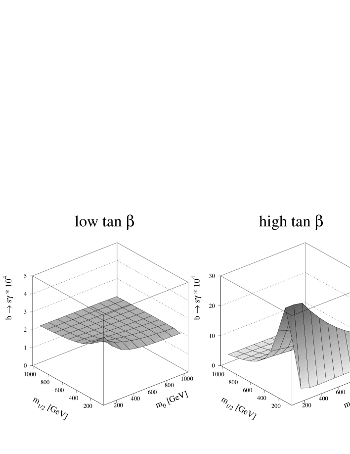
Figure 5: The branching ratio $b\rightarrow s\gamma$ as function of ${m_{0}}$ and ${m_{1/2}}$. Note that for large $\tan\beta$  only the region for ${m_{1/2}}<120$ GeV yields values compatible with experimental results.

The main contributions to $\chi^{2}$ are different for the different ${\tan\beta}$ regimes: for large ${\tan\beta}$ only small values of ${m_{1/2}}$ yield good fits, because of the simultaneous constraints of $BR(b\rightarrow s\gamma)$   and the large corrections to the b-quark mass, while at low ${\tan\beta}$ most of the ${m_{0}},{m_{1/2}}$ region is eliminated by the requirement that the relic density parameter $\Omega h^{2}$ should be below one. The calculated value of $BR(b\rightarrow s\gamma)$   and the relic density are shown as function of ${m_{0}}$ and ${m_{1/2}}$ in figs. 5 and 6, respectively.

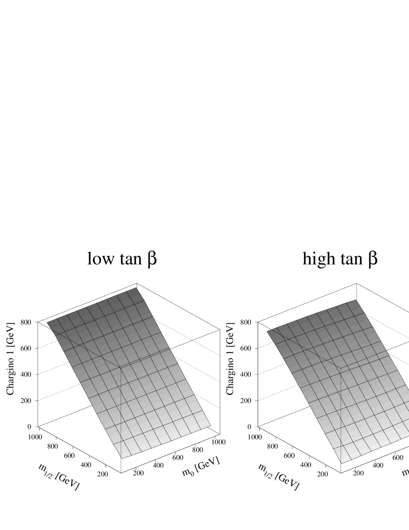
Figure 7: The lightest chargino mass as function of ${m_{0}}$ and ${m_{1/2}}$ for the low and high ${\tan\beta}$ scenario, respectively.

It should be noted the mass of the lightest chargino is about $0.7~{}-0.8~{}{m_{1/2}}$, as shown in fig. 7. The low value of ${m_{1/2}}$ for the best fit at large ${\tan\beta}$ implies a chargino mass of about 46 GeV (see table 3), which is just above the LEP I limit and should be detectable at LEP II or alternatively, the large ${\tan\beta}$ scenario can be excluded at LEP II, at least the minimal version. Of course, this conclusion depends sensitively on the $BR(b\rightarrow s\gamma)$   value. For large ${m_{1/2}}$ values, the prediction for this branching ratio is only 2 or 3 standard deviations above its experimental value (see fig. 5). In non-minimal models, e.g. ones with large splittings between $m_{1}$ and $m_{2}$ at the GUT scale, as studied by Borzumati et al. [61], the prediction for this branching ratio can be brought into agreement with experiment in the large ${m_{1/2}}$ region.

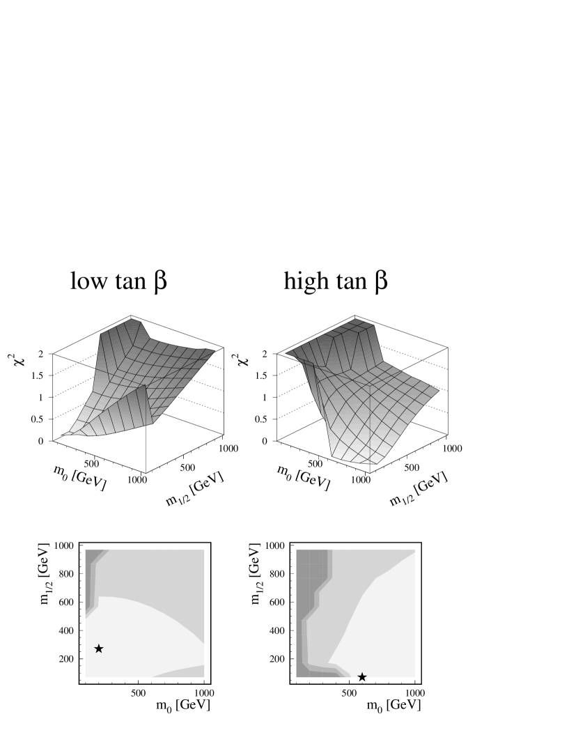
Figure 8: As fig. 3, but only including the constraints from unification and electroweak symmetry breaking.

Without the contraints from $b\rightarrow s\gamma$ and dark matter, large values of the SUSY scale cannot be excluded, since the $\chi^{2}$ from gauge and Yukawa coupling unification and electroweak symmetry breaking alone does not exclude these regions (see fig. 8), although there is a clear preference for the lighter SUSY scales.

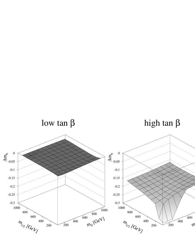
Figure 9: Corrections to the bottom quark mass from gluino, charged Higgses and Higgsino loop contributions in the MSSM as function of ${m_{0}}$ and ${m_{1/2}}$. Note the large negative corrections for $|\mu|<0$ in this case. Positive $\mu$-values would yield a large positive contribution, which excludes bottom-$\tau$ unification for most of the parameter space.

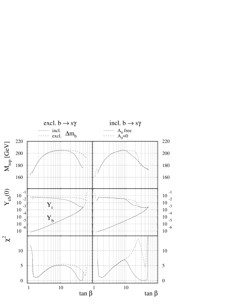
Figure 10: The top mass as function of ${\tan\beta}$ for ${m_{0}}=600$ and ${m_{1/2}}=70$ GeV. The various curves show the influence of the $\Delta m_{b}$ corrections, the $b\rightarrow s\gamma$ branching ratio and the trilinear couplings of the third generation ($A_{t}=A_{b}=A_{\tau}=A_{0}$) at the GUT scale. These effects are only important for the higher values of ${\tan\beta}$.

As mentioned in the previous section , at large ${\tan\beta}$ the b-mass has large, but finite corrections in the MSSM, as shown in fig. 9. Both, $BR(b\rightarrow s\gamma)$ and $\Delta m_{b}$ are sensitive functions of the mixing in the quark sector, given by the off-diagonal terms in the mass matrices (eqns. 2.2-2.2). Fitting both values simultaneously requires the trilinear coupling $A_{0}$ at the GUT scale to be non-zero, as shown in fig. 10: the $\chi^{2}$ for large ${\tan\beta}$ and $A_{0}=0$ is much worse than for fits, in which $A_{0}$ is left free. The influence of $\Delta m_{b}$ on the $m_{t}$ versus ${\tan\beta}$ solution is shown too on the left side. Note that the $\Delta m_{b}$ corrections improve the fit at the high ${\tan\beta}$ values. For the low ${\tan\beta}$ scenario the trilinear couplings were found to play a negligible role: varying them between $\pm 3{m_{0}}$ did not change the results significantly, since $A_{t}$ shows a fixed point behaviour in this case: its value at ${M_{Z}}$ is practically independent of the starting value at the GUT scale, as shown in fig. 11.

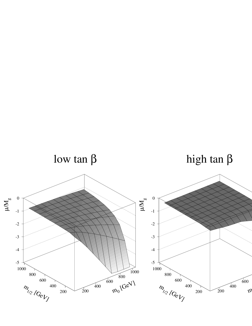
Figure 13: The ratio of $\mu({M_{Z}})$ and the gluino mass as function of ${m_{0}}$ and ${m_{1/2}}$ for the low and high ${\tan\beta}$ scenario, respectively.

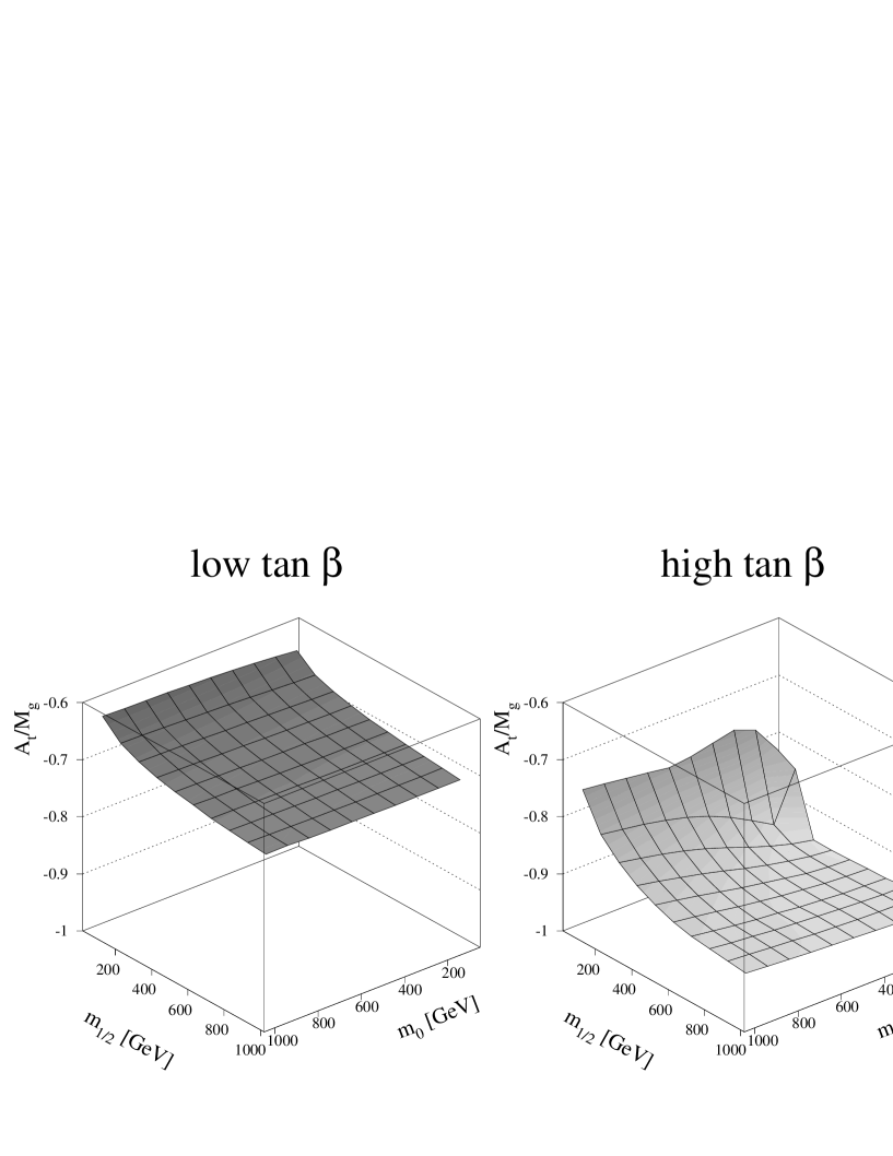
Figure 14: The ratio of $A_{t}({M_{Z}})$ and the gluino mass as function of ${m_{0}}$ and ${m_{1/2}}$ for the low and high ${\tan\beta}$ scenario, respectively.

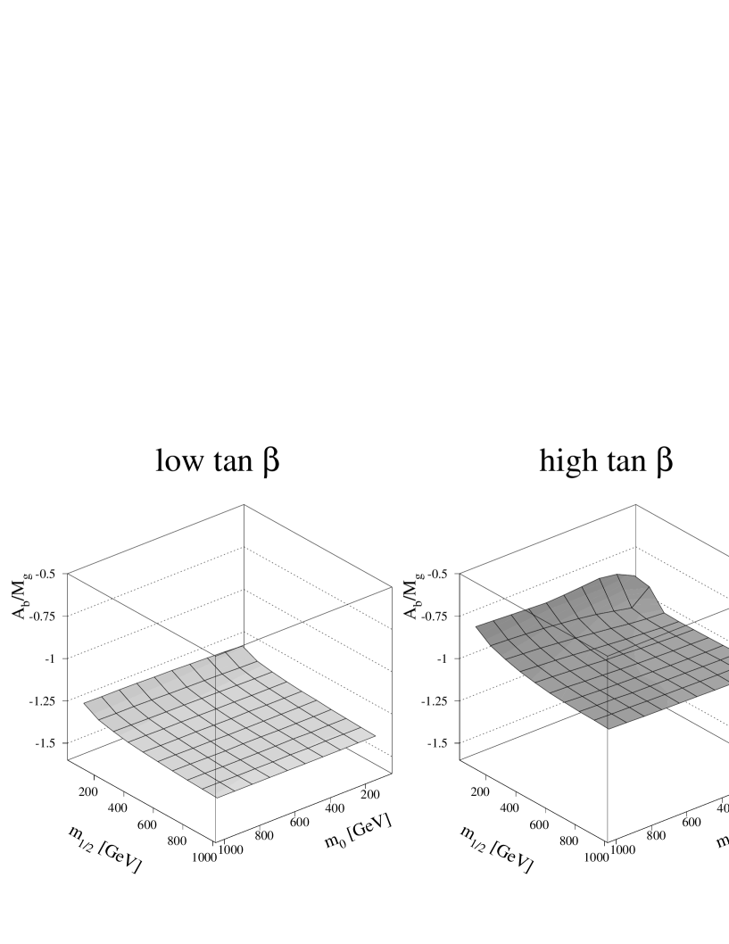
Figure 15: The ratio of $A_{b}({M_{Z}})$ and the gluino mass as function of ${m_{0}}$ and ${m_{1/2}}$ for the low and high ${\tan\beta}$ scenario, respectively.

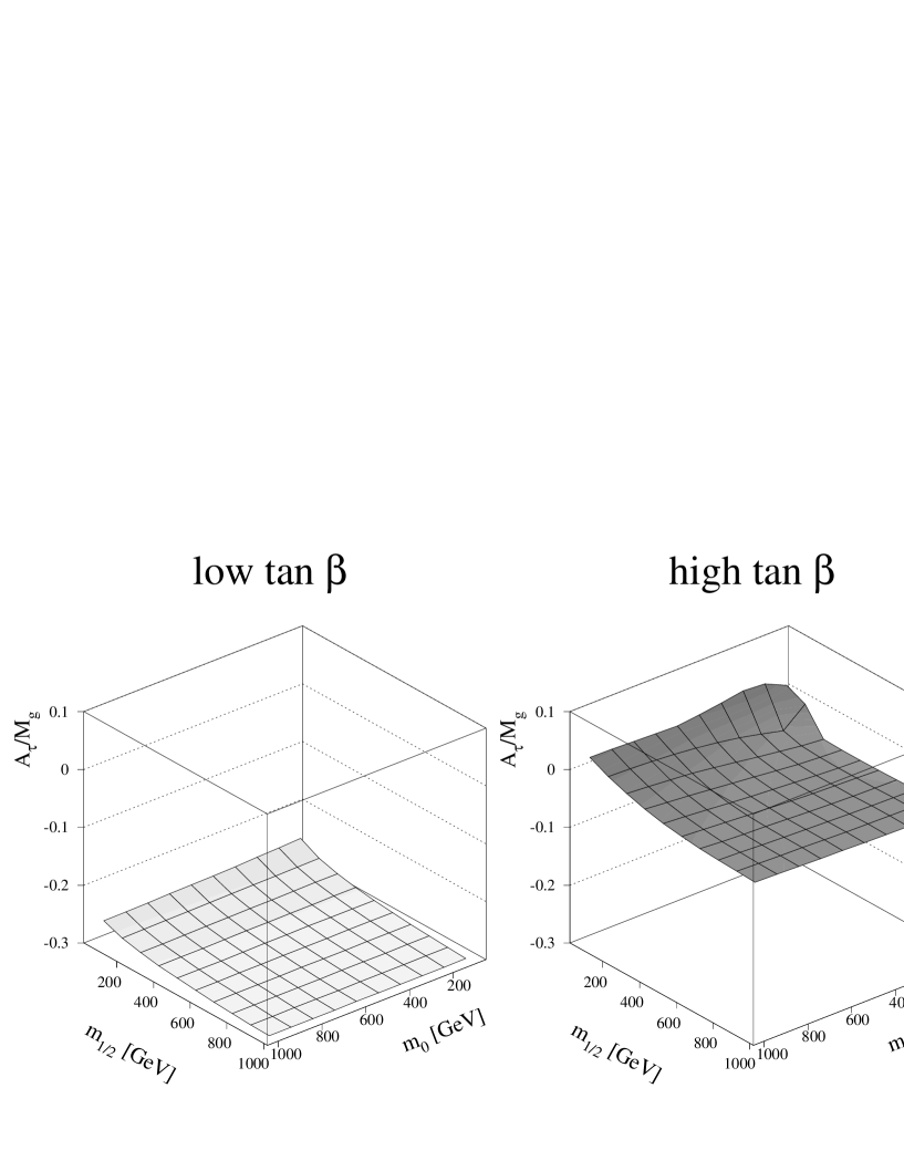
Figure 16: The ratio of $A_{\tau}({M_{Z}})$ and the gluino mass as function of ${m_{0}}$ and ${m_{1/2}}$ for the low and high ${\tan\beta}$ scenario, respectively.

The fitted values of the trilinear couplings and the Higgs mixing parameter $\mu$ are strongly correlated with ${m_{1/2}}$, so the ratio of these parameters at the electroweak scale and the gluino mass, which is about 2.7 ${m_{1/2}}$ as shown in fig. 14, is relatively constant and largely independent of ${m_{0}}$ (see figs. 13 - 16). Note from the figures that although the trilinear couplings $A_{t}$, $A_{b}$ and $A_{\tau}$ have equal values at the GUT scale, they are quite different at the electroweak scale due to the different RGE’s.

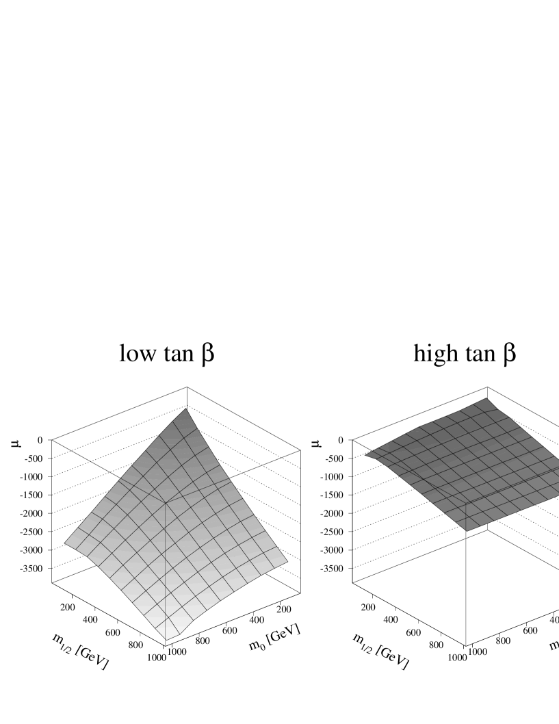
Figure 17: The Higgs mixing parameter $\mu_{0}$ at the GUT scale as function of ${m_{0}}$ and ${m_{1/2}}$ for the low and high ${\tan\beta}$ scenario, respectively.

The value of $\mu$ at the GUT scale is shown in fig. 17. Note the large values of $\mu$ at low ${\tan\beta}$, which implies little mixing in the neutralino sector and leads to eigenvalues of approximately $M_{1}$, $M_{2}$ and $\mu$ in the mass matrix (eq. 28). Since $M_{1}$ is the smallest value, the LSP will be almost purely a bino, which leads to strong constraints on the parameters from the lifetime of the universe.

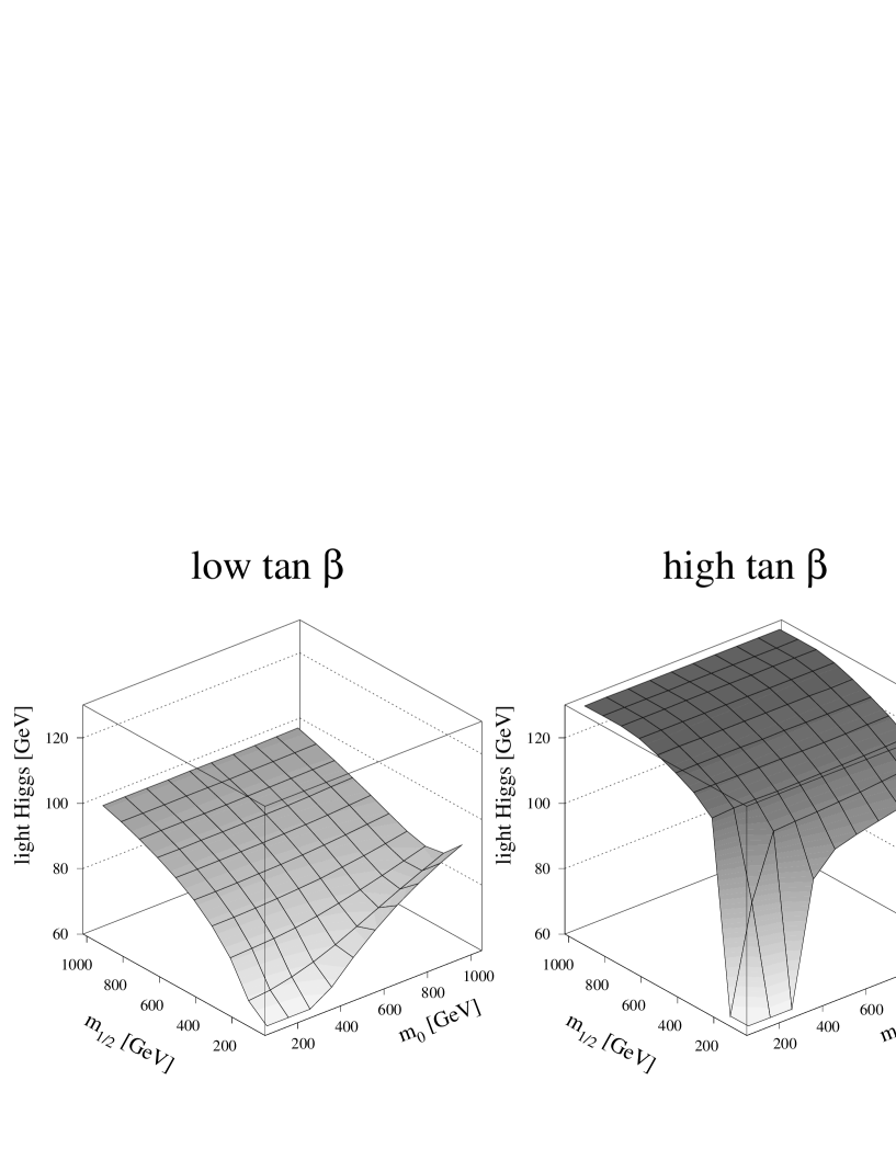
Figure 18: The mass of the lightest CP-even Higgs as function of ${m_{0}}$ and ${m_{1/2}}$ for the low and high ${\tan\beta}$ scenario, respectively. The sign of $\mu$ is negative, as required for the high ${\tan\beta}$ solution, but chosen negative for low ${\tan\beta}$.

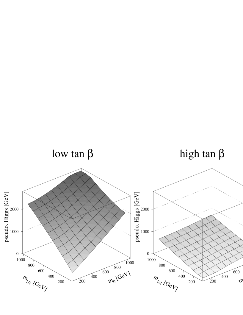
Figure 19: The mass of the CP-odd Higgs as function of ${m_{0}}$ and ${m_{1/2}}$ for the low and high ${\tan\beta}$ scenario, respectively.

Table 2 shows the parameters from the best fit and table 3 displays the corresponding SUSY masses. In figs. 18,19 the masses of the lightest CP-even and CP-odd Higgs bosons are shown for the whole parameter space for negative $\mu$-values. At each point a fit was performed to obtain the best solution for the GUT parameters. The mass of the lightest Higgs saturates at 100 GeV. For positive $\mu$-values and low ${\tan\beta}$ the maximum Higgs mass increases to 115 GeV.

For high ${\tan\beta}$ only negative $\mu$- values are allowed, since positive $\mu$-values yield a too high b-mass due to the large positive corrections in that case. The upper limit on the Higgs mass for positive $\mu$ and large ${\tan\beta}$ is about 130 GeV.

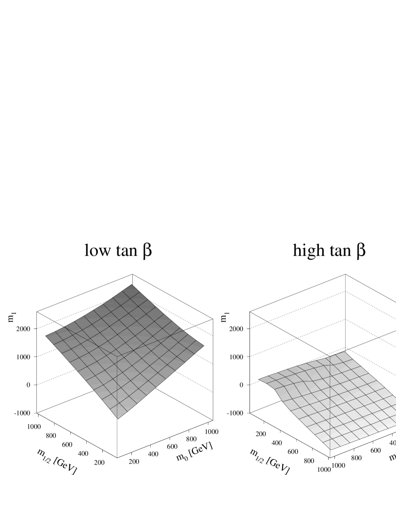
Figure 20: The mass $m_{1}$ in the Higgs potential at ${M_{Z}}$ (Born level) in GeV as function of ${m_{0}}$ and ${m_{1/2}}$ for the low and high ${\tan\beta}$ scenario, respectively.

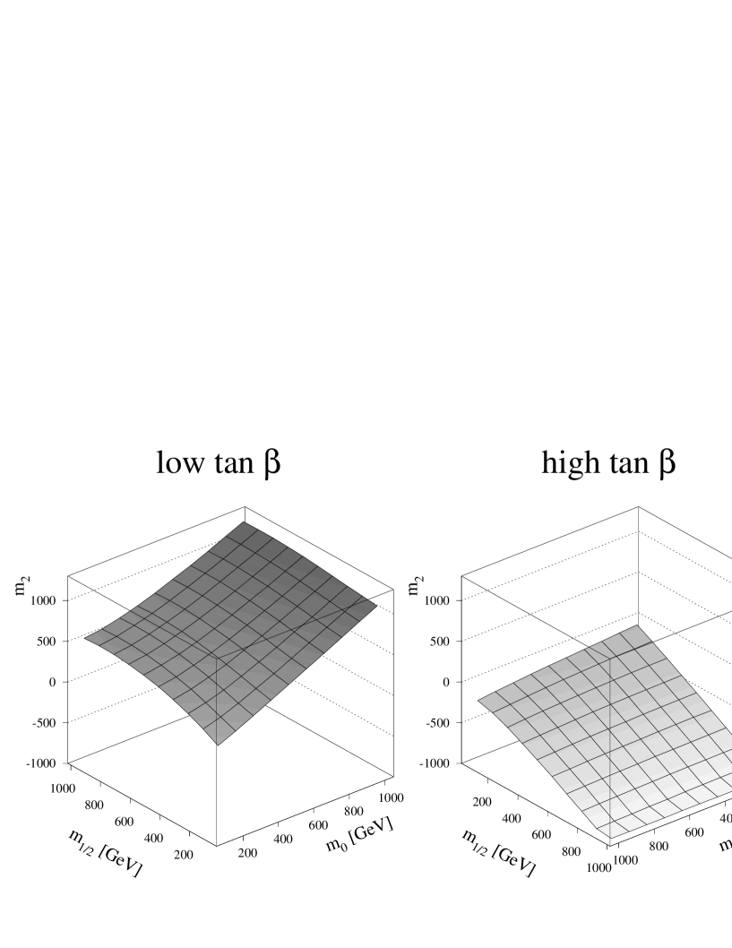
Figure 21: The mass $m_{2}$ in the Higgs potential at ${M_{Z}}$ (Born level) in GeV as function of ${m_{0}}$ and ${m_{1/2}}$ for the low and high ${\tan\beta}$ scenario, respectively.

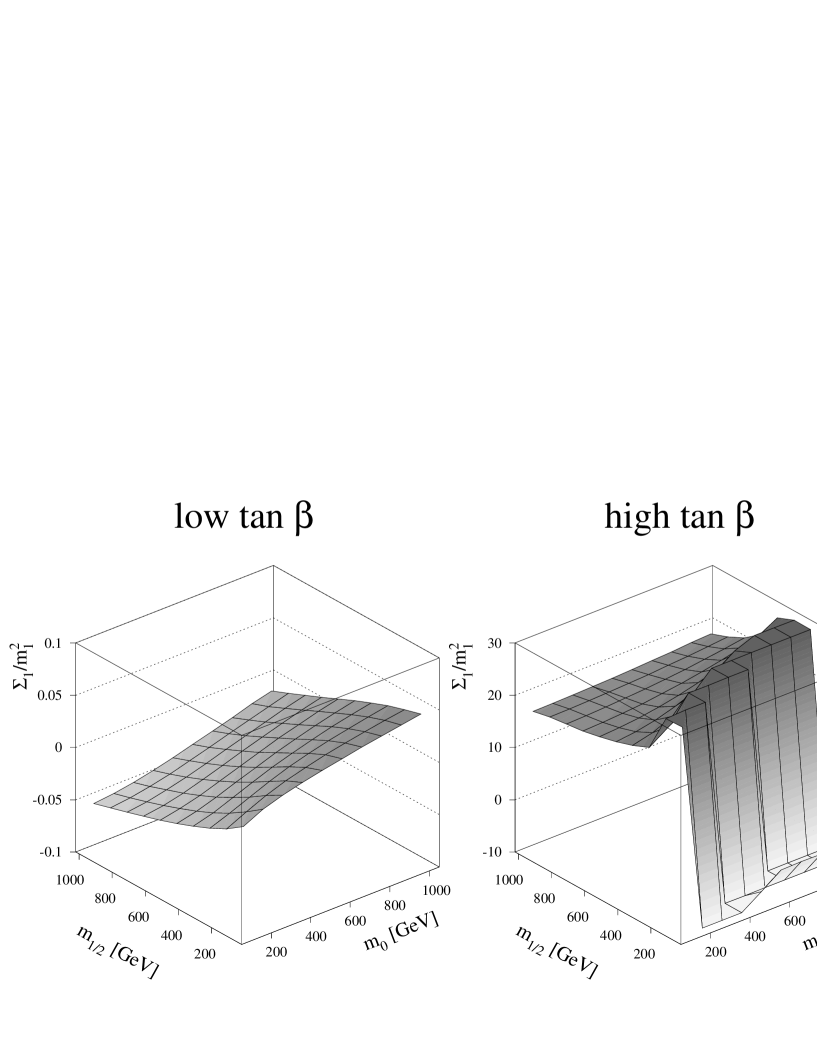
Figure 22: The one-loop corrections $\Sigma_{1}/m_{1}^{2}$ at ${M_{Z}}$ as function of ${m_{0}}$ and ${m_{1/2}}$ for the low and high ${\tan\beta}$ scenario, respectively.

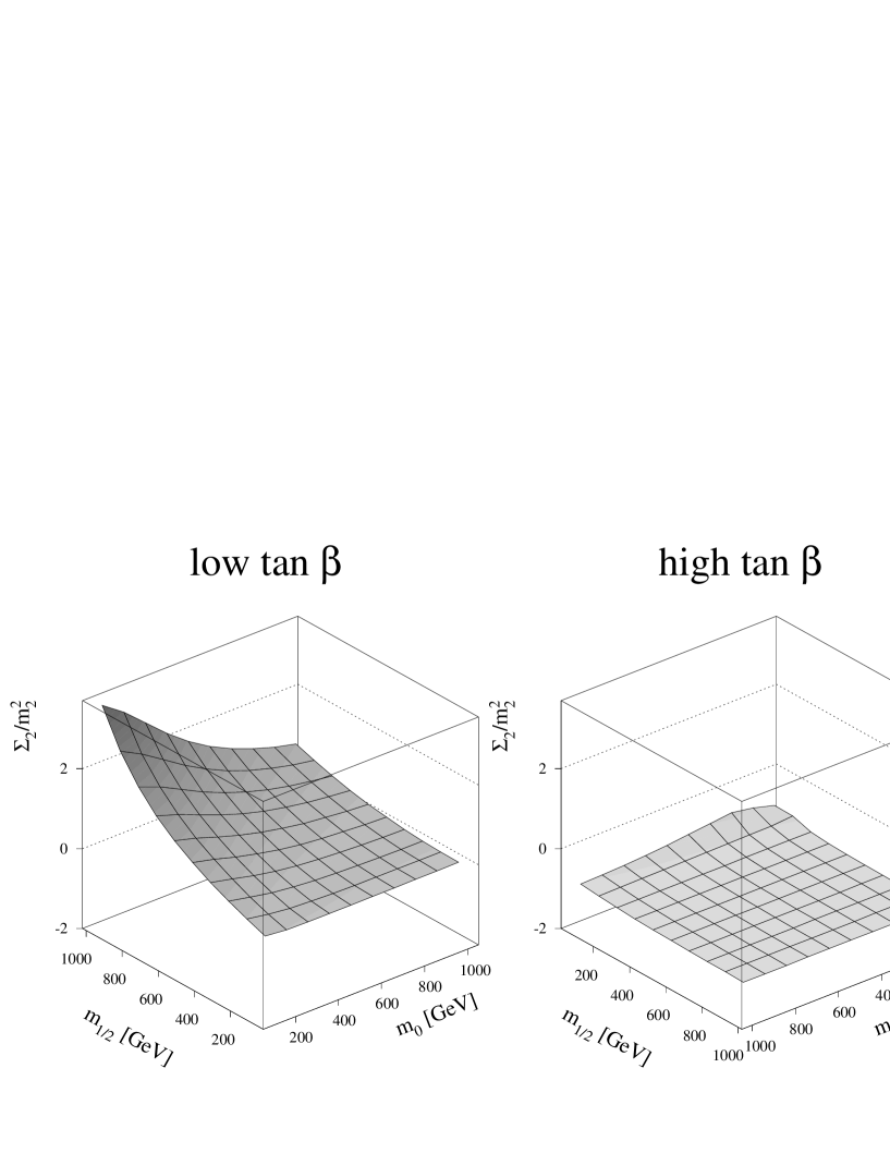
Figure 23: The one-loop corrections $\Sigma_{2}/m_{2}^{2}$ at ${M_{Z}}$ as function of ${m_{0}}$ and ${m_{1/2}}$ for the low and high ${\tan\beta}$ scenario, respectively.

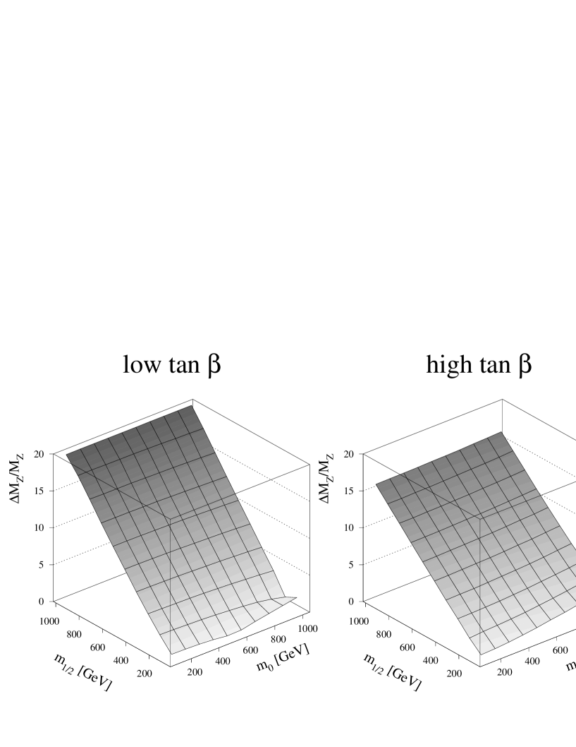
Figure 24: The one-loop radiative corrections $\Delta({M_{Z}})/{M_{Z}}$ as function of ${m_{0}}$ and ${m_{1/2}}$ for the low and high ${\tan\beta}$ scenario, respectively.

The upper limits for particles other than the lightest Higgs are considerable higher, unless restricted by some fine tuning argument: if the masses of the superpartners and the normal particles are different, the famous cancellation of quadratic divergencies in supersymmetry does not work anymore and the corrections to the Higgs masses quickly increase, as shown in figs. 20-23. These corrections lead to large corrections in the electroweak scale too (see fig. 24). It is a question of taste, if one considers the corrections large or small and if one should exclude some region of parameter space. In our opinion the fine tuning argument is difficult to use for a mass scale below 1 TeV, and the whole region up to 1 TeV should be considered, leading to quite large upper limits in case of the low ${\tan\beta}$ scenario[14].

5 Discovery Potential at LEP II

The programs SUSYGEN [70] and special SUSY routines [71] in ISAJET [72] have been used to calculate the production cross-sections for charginos, neutralinos and the lightest Higgses as function of the SUSY mass scales ${m_{0}}$ and ${m_{1/2}}$.

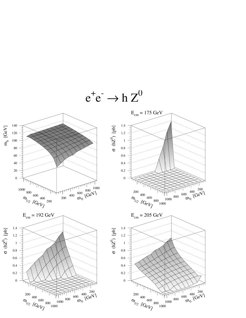
Figure 25: The Higgs mass as function of ${m_{0}}$ and ${m_{1/2}}$ for positive values of $\mu$ and low ${\tan\beta}$ (left top corner) and the main production cross sections for three different LEP II energies (175, 192 and 205 GeV). For negative $\mu$ values the Higgs mass is lighter (see fig. 7) and the cross sections about 50% larger.

Fig. 25 shows the mass of the lightest Higgs boson and the corresponding Higgs production cross sections at three LEP energies as functions of $m_{0}$ and $m_{1/2}$ for $\tan\beta=1.7$. The absolute value of the Higgs mass parameter $\mu$ was determined from the electroweak symmetry breaking condition; its sign was chosen positive. For negative $\mu$ values the cross sections are about 50% higher due to the lighter Higgs mass in that case (see fig. 18). Note the strong dependence of the cross section on the LEP centre-of-mass energy. At 205 GeV the whole CMSSM parameter space is covered, since at even higher values of the SUSY scale the Higgs mass hardly increases, as shown in the left top corner of fig. 25. For these results the large radiative corrections to $A_{t}$ and $A_{b}$ were taken into account, so they have nonzero values at the electroweak scale, typically $A_{t}=-0.7M_{\tilde{g}}$ and $A_{b}=-1.5M_{\tilde{g}}$ (see figs. 13 - 16). Note the fixed point behaviour of $A_{t}$ at low ${\tan\beta}$ values, as shown before in fig. 11.

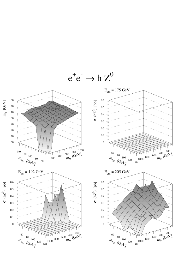
Figure 26: The Higgs mass as function of ${m_{0}}$ and ${m_{1/2}}$ for $\mu_{0}=-300$ GeV for ${\tan\beta}=46$ (left top corner) and the main production cross sections for three different LEP II energies (175, 192 and 205 GeV). $\mu$ was kept to a representative value (see fig. 17), since in most of the region the fit gave an unacceptable $\chi^{2}$, so $\mu$ could not be determined.

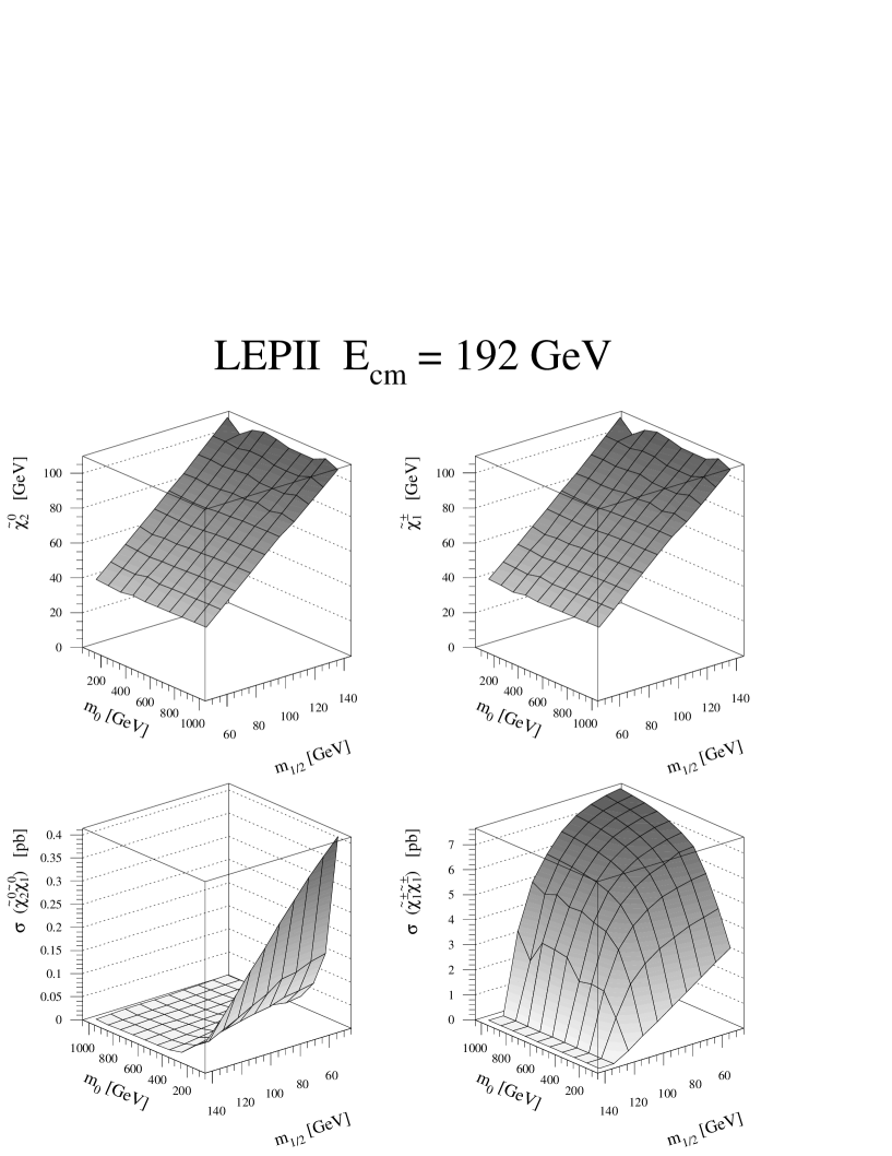
Figure 28: The masses of the second lightest neutralino and chargino masses as well as the production cross sections for $\mu_{0}=-300$ GeV and ${\tan\beta}=46$. $\mu$ was kept to a representative value (see fig. 17), since in most of the region the fit gave an unacceptable $\chi^{2}$, so $\mu$ could not be determined. Positive values of $\mu$ give similar results. The steep decrease in the chargino cross section at small values of ${m_{0}}$ is due to the light sneutrino in that region, which leads to a strong negative interference between s- and t-channel. Fortunately, the neutralino production is large there, as shown by the plot in the left bottom corner.

For large values of ${\tan\beta}$ only negative values of $\mu$ give acceptable fits, mainly because of the large corrections to the bottom mass, which prohibit tau-bottom unification for positive $\mu$. In this case the lightest Higgs mass becomes as large as 130 GeV for large values of the SUSY scales ${m_{0}}$ and ${m_{1/2}}$. However, if one includes the constraint from the radiative $b\rightarrow s\gamma$ decay, as measured by CLEO [21], only low values of $m_{1/2}$ give acceptable fits, in which case the remaining parameter space is largely accessible to a Higgs search, provided LEP II reaches its highest energies (see Fig. 26). The Higgs cross section is mainly a function of the Higgs mass and the center of mass energy. This dependency is shown in fig. 27 for some representative Higgs masses. In addition, the chargino and neutralino searches cover these regions, as shown in Fig. 28: even at a LEP II energy of 192 GeV searches for both, neutralino and chargino production, cover the region ${m_{1/2}}<110$ GeV, which is the region of interest for large $\tan\beta$  (see fig. 3).

6 Summary

In the Constrained Minimal Supersymmetric Model (CMSSM) the optimum values of the GUT scale parameters and the corresponding SUSY mass spectra for the low and high ${\tan\beta}$ scenario have been determined from a combined fit to the low energy data on couplings, quark and lepton masses of the third generation, the electroweak scale ${M_{Z}}$, $b\rightarrow s\gamma$ , and the lifetime of the universe.

At the highest LEP II energy of 205 GeV practically the whole parameter space of the CMSSM can be covered, both for the low and high ${\tan\beta}$ scenario, if one searches for Higgses, charginos and neutralinos. At the lower envisaged LEP II energy of 192 GeV only half of the parameter space for low ${\tan\beta}$ is accessible.

7 Acknowledgment

We thank Drs. D.I. Kazakov and A.V. Gladyshev for useful discussions. The research described in this publication was made possible in part by support from the Human Capital and Mobility Fund (Contract ERBCHRXCT 930345) from the European Community, and by support from the German Bundesministerium für Bildung und Forschung (BMBF) (Contract 05-6KA16P).

Figure 1: The top quark mass as function of ${\tan\beta}$ (top) for values of ${m_{0}},{m_{1/2}}$ optimized for low and high ${\tan\beta}$, as indicated by the dashed and solid lines, respectively. The middle part shows the corresponding values of the Yukawa coupling at the GUT scale and the lower part the obtained $\chi^{2}$ values. If the top constraint (${m_{t}}=179\pm 12$, horizontal band) is not applied, all values of ${\tan\beta}$ between 1.2 and 50 are allowed (thin dotted lines at the bottom), but if the top mass is constrained to the experimental value, only the regions $1<{\tan\beta}<3$ and $15<{\tan\beta}<50$ are allowed.

Figure 2: The running of the parameters $m_{1}$ and $m_{2}$ in the Higgs potential (top) and Yukawacouplings of top and bottom quarks (bottom).

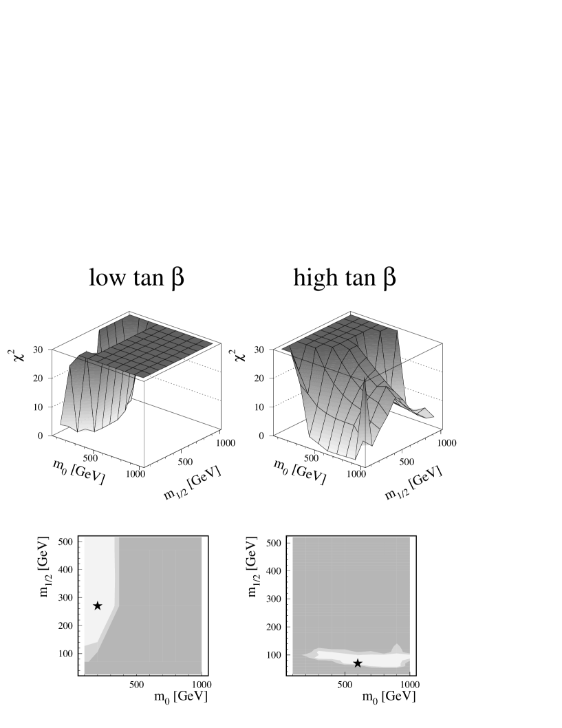
Figure 3: The total $\chi^{2}$-distribution for low and high ${\tan\beta}$ solutions (top) as well as the projections (bottom). The different shades indicate steps of $\Delta\chi^{2}=2$, so basically only the light shaded region is allowed. The stars indicate the optimum solution.

Figure 4: The running of the particle masses and the $\mu$ parameter for low and high ${\tan\beta}$ values.

Figure 6: The relic density as function of ${m_{0}}$ and ${m_{1/2}}$ for the low and high ${\tan\beta}$ scenario, respectively.

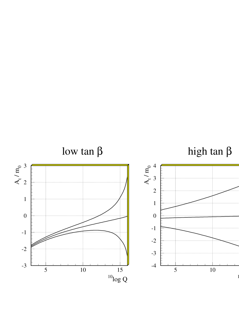
Figure 11: The running of $A_{t}$. The values of (${m_{0}},{m_{1/2}}$) were choosen to be (200,270) and (600,70) GeV for the low and high ${\tan\beta}$ scenario, respectively. However, the fixed point behaviour is found for other values of ${m_{0}},{m_{1/2}}$ too: at low values of ${\tan\beta}$ a strong convergence to a single value is found, while for high values this tendency is much less pronounced.

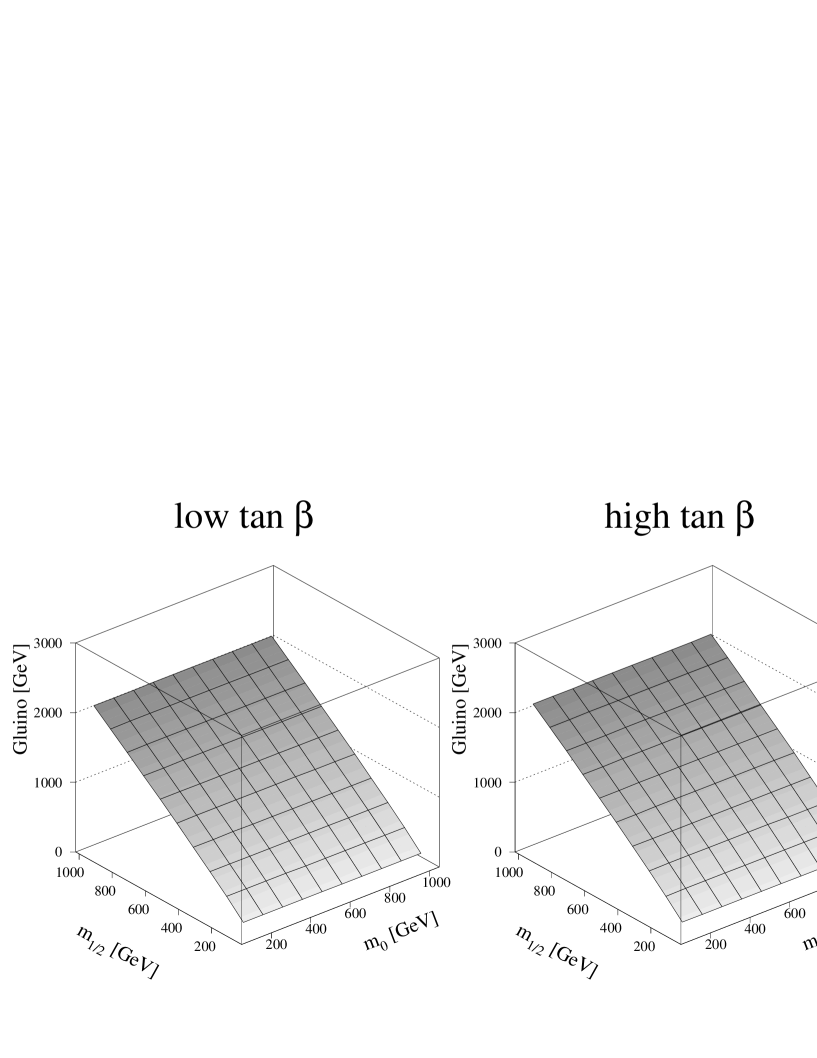
Figure 12: The gluino mass as function of ${m_{0}}$ and ${m_{1/2}}$ for the low and high ${\tan\beta}$ scenario, respectively.

Figure 27: The cross section as function of the center of mass energy for different Higgs masses, as indicated by the numbers (in GeV). The upper limit on the Higgs mass is $\approx$ 115 GeV. (see figs. 25 and 26).

References

-
[1]
P. Fayet, Phys. Lett. B64 (1976) 159; ibid. B60 (1977)
489;
S. Dimopoulos, H. Georgi, Nucl. Phys. B193 (1981) 150;
L. E. Ibáñez, G. G. Ross, Phys. Lett. B105 (1981) 435;
S. Dimopoulos, S. Raby, F. Wilczek, Phys. Rev. D24 (1981) 1681;
N. Sakai, Z. Phys. C11 (1981) 153;
A. H. Chamseddine, R. Arnowitt and P. Nath, Phys. Rev. Lett. 49 (1982) 970. - [2] J. Ellis, S. Kelley, and D. V. Nanopoulos. Nucl. Phys. B373 (1992) 55.
- [3] U. Amaldi, W. de Boer, and H. Fürstenau. Phys. Lett. B260 (1991) 447.
- [4] P. Langacker and M. Luo. Phys. Rev. D44 (1991) 817.
-
[5]
For references see the review papers:
H.-P. Nilles, Phys. Rep. 110 (1984) 1;
H.E. Haber, G.L. Kane, Phys. Rep. 117 (1985) 75;
A.B. Lahanas and D.V. Nanopoulos, Phys. Rep. 145 (1987) 1;
R. Barbieri, Riv. Nuo. Cim. 11 (1988) 1. - [6] G. G. Ross and R. G. Roberts. Nucl. Phys. B377 (1992) 571.
- [7] M. Carena, S. Pokorski, and C. E. M. Wagner. Nucl. Phys. B406 (1993) 59.
- [8] V. Barger, M. S. Berger, and P. Ohmann. Phys. Rev. D47 (1993) 1093.
- [9] M. Olechowsi and S. Pokorski. Nucl. Phys. B404 (1993) 590.
- [10] P.H. Chankowski et al. IFT-95-9, MPI-PTH-95-58 and ref. therein.
- [11] P. Langacker and N. Polonsky. Phys. Rev. D49 (1994) 1454; UPR-0642-T and ref. therein.
- [12] J. L. Lopez, D.V. Nanopoulos, and A. Zichichi. Progr. in Nucl. and Particle Phys., 33 (1994) 303 and ref. therein.
- [13] W. de Boer. Progr. in Nucl. and Particle Phys., 33 (1994) 201.
- [14] W. de Boer, R. Ehret, and D. Kazakov. Phys. Lett. B334 (1994) 220.
-
[15]
J. L. Lopez, D.V. Nanopoulos, A. Zichichi, CTP-TAMU-40-93 (1993);
CTP-TAMU-33-93 (1993); CERN-TH-6934-93 (1993); CERN-TH-6926-93-REV (1993);
CERN-TH-6903-93 (1993);
J. L. Lopez, et al., Phys. Lett. B306 (1993) 73. -
[16]
S.P. Martin and P. Ramond, Phys. Rev. D48 (1993) 5365
D.J. Castano, E.J. Piard, and P. Ramond, Phys. Rev. D49 (1994) 4882. - [17] G. L. Kane, C. Kolda, L. Roszkowski, and J. D. Wells. Phys. Rev. D49 (1994) 6173.
- [18] C. Kolda, L. Roszkowski, and J. D. Wells and G. L. Kane. Phys. Rev. D50 (1994) 3498.
- [19] M. Carena and C. E. M. Wagner. CERN-TH-7393-94 and ref. therein.
- [20] M. Carena, M. Olechowski, S. Pokorski, and C. E. M. Wagner. Nucl. Phys. 419 (1994) 213.
- [21] R. Ammar et al. CLEO-Collaboration. Phys. Rev. Lett. 74 (1995) 2885.
-
[22]
R. Arnowitt and P. Nath.
Phys. Rev. Lett. 69 (1992) 725; Phys. Lett. B287
(1992) 89; Phys. Lett. B289 (1992) 368; Phys. Lett. B299 (1993)
58, ERRATUM-ibid. B307 (1993) 403; Phys. Rev. Lett. 70 (1993)
3696;
CTP-TAMU-23/93 (1993). and references therein. - [23] P. Langacker. Univ. of Penn. Preprint, UPR-0539-T (1992).
- [24] D.V. Nanopoulos J. Ellis, J.L. Lopez. Phys. Lett. B252 (1990) 53.
- [25] D.I. Kazakov et al., . Contr. paper to the EPS Conf., Brussels, (1995).
-
[26]
Yu.A. Gol’fand and E.P. Likhtman, JETP Lett. 13 (1971) 323;
D.V. Volkov and V.P. Akulow, Phys. Lett. 46b (1971) 323;
J. Wess and B. Zumino, Nucl. Phys. B70 (1974) 39;
J. Wess and B. Zumino, Phys. Lett. 49B (1974) 52;
S. Ferrara, J. Wess, and B. Zumino., Phys. Lett. 51B (1974) 239;
J. Iliopoulos and B. Zumino, Nucl. Phys. B76 (1974) 310. - [27] R. Arnowitt and P. Nath. Phys. Rev. D46 (1992) 3981.
-
[28]
J. Ellis, G. Ridolfi, and F. Zwirner.
Phys. Lett. B257 (1991) 83;
Phys. Lett. B262 (1991) 477. - [29] A. Brignole, J. Ellis, G. Ridolfi, and F. Zwirner. Phys. Lett. B271 (1991) 123.
- [30] M. Drees and M. M. Nojiri. Phys. Rev. D45 (1992) 2482.
- [31] Z. Kunszt and F. Zwirner. Nucl. Phys. B 385 (1992) 3.
- [32] J. R. Espinosa, M. Quirós, and F. Zwirner. Phys. Lett. B307 (1993) 106.
-
[33]
P. H. Chankowski, S. Pokorski, and J. Rosiek.
Nucl. Phys. B423 (1994) 437;
MPI-PH-92-116 (1992); MPI-PH-92-116-ERR (1992). -
[34]
U. Amaldi, W. de Boer, P. H. Frampton, H. Fürstenau, and J.T. Liu.
Phys. Lett. B281 (1992) 374. -
[35]
H. Murayama and T. Yanagida, Mod. Phys. Lett. A7 (1992) 147;
T. G. Rizzo, Phys. Rev. D45 (1992) 3903;
T. Moroi, H. Murayama and T. Yanagida, Phys. Rev. D48 (1993) 2995. -
[36]
G. ’t Hooft, Nucl. Phys. B61, (1973) 455;
W. A. Bardeen, A. Buras, D. Duke and T. Muta, Phys. Rev. D 18, (1978) 3998. - [37] The LEP Collaborations: ALEPH, DELPHI, L3 and OPAL and the LEP electroweak Working Group;. Phys. Lett. 276B (1992) 247;. Updates are given in CERN/PPE/93-157, CERN/PPE/94-187 and LEPEWWG/95-01 (see also ALEPH 95-038, DELPHI 95-37, L3 Note 1736 and OPAL TN284.
- [38] Review of Particle Properties. Phys. Rev. D50 (1994).
- [39] CDF Collab., F. Abe, et al. Phys. Rev. Lett. 74 (1995) 2626.
- [40] D0 Collab., S. Abachi, et al. Phys. Rev. Lett. 74 (1995) 2632.
- [41] G. Degrassi, S. Fanchiotti, and A. Sirlin. Nucl. Phys. B351 (1991) 49.
- [42] S. Eidelmann and F. Jegerlehner. Hadronic contributions to (g-2) of leptons and to the effective fine structure constant , PSI Preprint PSI-PR-95-1.
- [43] I. Antoniadis, C. Kounnas, and K. Tamvakis. Phys. Lett. 119B (1982) 377.
- [44] B. Pendleton and G.G. Ross. Phys. Lett. B98 (1981) 291;.
- [45] V. Barger, M. S. Berger, P. Ohmann, and R. J. N. Phillips. Phys. Lett. B314 (1993) 351.
- [46] P. Langacker and N. Polonski. Univ. of Pennsylvania Preprint UPR-0556-T, (1993).
- [47] S. Kelley, J. L. Lopez, and D.V. Nanopoulos. Phys. Lett. B274 (1992) 387.
- [48] M. Carena, , M. Olechowski, S. Pokorski, and C. E. M. Wagner. Nucl. Phys. B426 (1994) 269.
- [49] H. Arason et al. Phys. Rev. Lett. 67 (1991) 2933.
-
[50]
J. Gasser and H. Leutwyler, Phys. Rep. 87C (1982) 77;
S. Narison, Phys. Lett. B216 (1989) 191;
N. Gray, D.J. Broadhurst, W. Grafe and K. Schilcher, Z. Phys. C48 (1990) 673. - [51] R. Hempfling. Phys. Rev. D49 (1994) 6168.
- [52] U. Sarid L. Hall, R. Rattazzi. LBL-33997,UCB-PTH-93/14, Phys. Rev. D50(1994)7048.
- [53] K.G. Chetyrkin and A. Kwiatkowski. Phys. Lett. B305 (1993) 285.
- [54] D. Buskulic et al., ALEPH Coll. Phys. Lett. B313 (1993) 312.
- [55] A. Sopczak. CERN-PPE/94-73,Lisbon Fall School 1993.
- [56] F. Borzumati, Z. Phys. C63 (1995) 291.
-
[57]
S. Bertolini, F. Borzumati, A.Masiero, and G. Ridolfi, Nucl. Phys.
B353 (1991) 591 and references therein;
N. Oshimo, Nucl. Phys. B404 (1993) 20. - [58] A.J. Buras et al. Nucl. Phys. B424(1994)374.
-
[59]
R. Barbieri and G. Giudice, Phys. Lett. B309 (1993) 86;
R. Garisto and J.N. Ng, Phys. Lett. B315 (1993) 372. - [60] A. Ali and C. Greub. Z. Phys. C60 (1993) 433.
- [61] F.M. Borzumati, M. Olechowski and S. Pokorski, Phys. Lett. B349 (1995) 311.
- [62] J. L. Lopez, D.V. Nanopoulos, G. T. Park, Phys. Rev. D48 (1993) 974; J.L. Lopez et al., Phys. Rev. D51 (1995) 147.
-
[63]
J.L. Hewett, Phys. Rev. Lett. 70 (1993) 1045;
V. Barger, M.S. Berger, and R.J.N. Phillips, Phys. Rev. Lett. 70 (1993) 1368;
M.A. Diaz, Phys. Lett. B304 (1993) 278. - [64] G. Börner. The early Universe,. Springer Verlag, (1991).
- [65] E.W. Kolb and M.S. Turner. The early Universe,. Addison-Wesley, (1990).
-
[66]
G. Steigman, K.A. Olive, D.N. Schramm, M.S. Turner, Phys. Lett. B176 (1986) 33;
J. Ellis, K. Enquist, D.V. Nanopoulos, S. Sarkar, Phys. Lett. B167 (1986) 457;
G. Gelmini and P. Gondolo, Nucl. Phys. 360 (1991) 145. -
[67]
M. Drees and M. M. Nojiri, Phys. Rev. D47 (1993) 376;
J. L. Lopez, D.V. Nanopoulos, and H. Pois, Phys. Rev. D47 (1993) 2468;
P. Nath and R. Arnowitt, Phys. Rev. Lett. 70 (1993) 3696;
J. L. Lopez, D.V. Nanopoulos, and K. Yuan, Phys. Rev. D48 (1993) 2766. - [68] L. Roszkowski, Univ. of Michigan Preprint, UM-TH-93-06; UM-TH-94-02.
- [69] J. Ellis et al., Nucl. Phys. B238 (1984) 453.
- [70] S. Katsanevas. SUSYGEN,private communication.
- [71] Baer et. al. Int. Journ. of mod. phys.Vol.4,16(1989)4111.
- [72] F.E Paige and S.D. Protopopescu. ISAJET7.11,Fermilab.