Hadron Spectra for Semileptonic Heavy Quark Decay

Abstract

We calculate the leading perturbative and power corrections to the hadronic invariant mass and energy spectra in semileptonic heavy hadron decays. We apply our results to the $B$ system. Moments of the invariant mass spectrum, which vanish in the parton model, probe gluon bremsstrahlung and nonperturbative effects. Combining our results with recent data on $B$ meson branching ratios, we obtain a lower bound $\bar{\Lambda}>410\,{\rm MeV}$ and an upper bound $m_{b}^{\rm pole}<4.89\,$GeV. The Brodsky-Lepage-Mackenzie scale setting procedure suggests that higher order perturbative corrections to the first moment of the hadronic invariant mass spectrum are small for bottom decay, and even tractable for charm decay.

I Introduction

Our understanding of inclusive decays of hadrons containing at least one heavy quark has improved greatly over the last few years. The energy released during semileptonic or radiative decay of heavy hadrons is much larger than the scale $\Lambda_{\rm QCD}$ of the strong interactions, and therefore an operator product expansion (OPE) exists for some observables in these decays, including rates and differential spectra [1, 2]. The leading power corrections to the rates and lepton differential spectra for semileptonic decays of heavy hadrons[3, 4, 5, 6] have been studied extensively, as have the power corrections to radiative decays [7].

A major result of this analysis is that, except in regions where the expansion becomes singular such as the endpoint of the electron spectrum in semileptonic $b\rightarrow u$ decay, the corrections to the parton model are quite small, suppressed by ${\cal O}(\Lambda_{\rm QCD}^{2}/m_{b}^{2})$. While this does mean that the parton model is quite successful, it makes it difficult to test quantitatively the corrections given by the OPE. In particular, if quark/hadron duality does not hold in this energy regime, one would expect to see corrections to the parton model which could not be accounted for by the leading perturbative and $1/m_{Q}$ corrections. Shifman has recently criticized the related OPE analysis of $\tau$ decay on the basis that violations of duality in the Minkowski regime introduce large corrections which are not seen at any finite order in the OPE [8].

In this paper we suggest that hadronic variables, in particular moments of the invariant mass spectrum ${\rm d}\Gamma/{\rm d}s_{H}$ and the hadron energy spectrum ${\rm d}\Gamma/{\rm d}E_{H}$, provide a useful testing ground for the OPE. This is similar to the analogous suggestion, and analysis, for semileptonic $\tau$ decays [9, 10]. However, unlike the case for $\tau$ decays, at tree level the final hadronic state at the parton level consists of a single quark. Therefore at lowest order in the OPE the final hadronic state has fixed invariant mass $s_{H}=m_{q}^{2}$, and positive moments of $(s_{H}-m_{q}^{2})$, which are calculable as a double expansion in $\alpha_{s}(m_{b})$ and $1/m_{b}$, directly probe physics beyond the parton model. Similarly, at leading order in the OPE the maximum hadron energy is $(m_{b}^{2}+m_{q}^{2})/2m_{b}$ (when the quark $q$ recoils back-to-back with the leptons); the region above this endpoint is populated only by gluon bremsstrahlung and nonperturbative effects.

In this paper we calculate the corrections to the parton model results for these observables, up to ${\cal O}(1/m_{b}^{2},\alpha_{s}/m_{b})$. As discussed in Ref. [11], although the leading power corrections to leptonic variables arise at ${\cal O}(1/m_{b}^{2})$, for kinematic reasons the leading power corrections to moments of the invariant mass spectrum arise at ${\cal O}(1/m_{b})$. The ${\cal O}(1/m_{b}^{2})$ corrections to the differential hadronic energy spectrum were first examined in Ref. [12]; however, we disagree with the results presented in that work. We also use the results of Ref. [13], in which the one-loop corrections to the hadron energy spectrum were calculated. We combine our results with recent data on $B$ meson branching ratios to obtain a lower bound on the nonperturbative parameter $\bar{\Lambda}$, which is the leading contribution to the difference between heavy quark and heavy meson masses.

Finally, using the BLM prescription [14] to estimate the size of the two-loop perturbative corrections to the moments of the invariant mass spectrum, we demonstrate that the first moment appears to have a well-behaved perturbative expansion not only for $B$ decays, but also for $D$ decays, when the results are expressed in terms of physical observables. This suggests that studying hadronic observables in semileptonic decays of charmed hadrons, which are dominated by only two or three resonances, may shed some insight into the applicability of quark/hadron duality at low energies.

II Kinematics

We start by introducing the kinematic variables describing the final state hadrons. For definiteness, we will consider semileptonic $B$ decay, although the analysis extends simply to the decays of charmed hadrons.

The kinematics of the inclusive process $B\to X_{q}\ell\nu$ is shown in Fig. 1.

FIG. 1.: The kinematics for $B\to X_{q}\ell\nu$.

The four-momentum of the $B$ meson is $P_{B}^{\mu}=m_{B}v^{\mu}$, and $q^{\mu}$ is the four-momentum of the lepton pair. We write the four-momentum of the $b$ quark as $P_{b}^{\mu}$, and assign the heavy quark the same four-velocity $v^{\mu}$ as the heavy meson. The total energy of the leptons in the $B$ rest frame is $v\cdot q$, and their invariant mass is $q^{2}$. It is convenient to define dimensionless parton level quantities $\hat{E}_{0}$ and $\hat{s}_{0}$,

$$\hat{E}_{0} = v\cdot(P_{b}-q)/m_{b}=1-v\cdot\hat{q}\,,$$ (1)

$$\hat{s}_{0} = (P_{b}-q)^{2}/m_{b}^{2}=1-2v\cdot\hat{q}+\hat{q}^{2}\,,$$ (2)

where $\hat{q}^{\mu}=q^{\mu}/m_{b}$. At leading order in $1/m_{b}$, $\hat{E}_{0}$ and $\hat{s}_{0}$ are simply the scaled energy and squared invariant mass of the final hadronic state. However, since they are scaled by the $b$ quark mass, this identification does not hold at subleading order in $1/m_{b}$. Instead, they are related to the physical hadronic energy and squared invariant mass,

$$E_{H} = v\cdot(P_{B}-q)=m_{B}-v\cdot q\,,$$ (3)

$$s_{H} = (P_{B}-q)^{2}=m_{B}^{2}-2m_{B}v\cdot q+q^{2}\,,$$ (4)

through

$$E_{H} = \bar{\Lambda}-{\lambda_{1}+3\lambda_{2}\over 2m_{B}}+\left(m_{B}-\bar{\Lambda}+{\lambda_{1}+3\lambda_{2}\over 2m_{B}}\right)\hat{E}_{0}+\dots\,,$$ (5)

$$s_{H} = m_{q}^{2}+\bar{\Lambda}^{2}+(m_{B}^{2}-2\bar{\Lambda}m_{B}+\bar{\Lambda}^{2}+\lambda_{1}+3\lambda_{2})\,(\hat{s}_{0}-\hat{m}_{q}^{2})$$ (7)

$$\qquad\qquad\mbox{}+(2\bar{\Lambda}m_{B}-2\Lambda^{2}-\lambda_{1}-3\lambda_{2})\hat{E}_{0}+\dots\,,$$

where $\hat{m}_{q}=m_{q}/m_{b}$, and the ellipses denote terms higher order in $1/m_{b}$. The quantities $\bar{\Lambda}$, $\lambda_{1}$ and $\lambda_{2}$ arise in the relationship between the quark and meson masses [15, 16],

$$m_{B} = m_{b}+\bar{\Lambda}-{\lambda_{1}+3\lambda_{2}\over 2m_{b}}+\dots\,,$$ (8)

$$m_{B^{*}} = m_{b}+\bar{\Lambda}-{\lambda_{1}-\lambda_{2}\over 2m_{b}}+\dots\,.$$ (9)

From the measured $B$–$B^{*}$ mass splitting, $\lambda_{2}\simeq 0.12\,{\rm GeV}^{2}$. We note that in contrast to the lepton spectra, there are $1/m_{b}$ corrections both to the physical hadronic invariant mass spectrum and to the physical hadronic energy spectrum, although these corrections are absent for the $\hat{s}_{0}$ and $\hat{E}_{0}$ spectra [11].

While the complete shape of the $\hat{E}_{0}$ spectrum may be calculated (away from the parton model endpoint $\hat{E}_{0}={1\over 2}(1+\hat{m}_{q}^{2})$) with the standard OPE analysis, only suitably averaged features, such as moments, of the $\hat{s}_{0}$ spectrum may be computed reliably. The difference arises because each point of the $\hat{E}_{0}$ spectrum receives contributions from states of different invariant masses, making the process inclusive, whereas by definition each point of the $\hat{s}_{0}$ spectrum only receives contributions from states of a single invariant mass. This may be seen explicitly by carrying out the usual OPE analysis for inclusive decays in the variables $\hat{s}_{0}$ and $\hat{E}_{0}$, instead of the usual leptonic variables $v\cdot\hat{q}$ and $\hat{q}^{2}$.

The inclusive $B$ meson decay rate is given by

$$\Gamma(B\to X_{q}\ell\nu)\sim\int{\rm d}\hat{s}_{0}\,{\rm d}\hat{E}_{0}\,\sqrt{\hat{E}_{0}^{2}-\hat{s}_{0}}L_{\mu\nu}(\hat{s}_{0},\hat{E}_{0})W^{\mu\nu}(\hat{s}_{0},\hat{E}_{0})\,,$$ (10)

where $L_{\mu\nu}$ is the spin summed lepton tensor $L_{\mu\nu}\propto(q_{\mu}q_{\nu}-g_{\mu\nu}q^{2})$. Using the optical theorem, the nonperturbative hadronic tensor $W^{\mu\nu}$ is related to the imaginary part of the forward scattering amplitude [1, 2],

$$W^{\mu\nu} = \sum_{X}\langle B|\,J_{h}^{\mu\dagger}\,|X\rangle\langle X|\,J_{h}^{\nu}\,|B\rangle(2\pi)^{4}\delta^{4}(P_{B}-P_{X}-q)$$ (11)

$$= -2\,{\rm Im}\,\langle B|\,i\int{\rm d}x\,e^{-iq\cdot x}\,T\left[J_{h}^{\mu\dagger}(x)J_{h}^{\nu}(0)\right]\,|B\rangle$$ (12)

$$\equiv 2\,{\rm Im}\,T^{\mu\nu}\,$$ (13)

where $J^{\mu}_{h}=\overline{q}\gamma^{\mu}{1\over 2}(1-\gamma_{5})b$. The time-ordered product $T^{\mu\nu}$ may be written via an operator product expansion as a power series in $\alpha_{s}(m_{b})$ and $1/m_{b}$.

In the $v\cdot\hat{q}$ plane, for fixed $\hat{q}^{2}$, the correlator $T^{\mu\nu}$ has the analytic structure shown in Fig. 2a, as discussed in Ref. [2].

FIG. 2.: The analytic structure of $T^{\mu\nu}$, (a) in the $v\cdot\hat{q}$ plane, with $\hat{q}^{2}$ fixed, and (b) in the $\hat{s}_{0}$ plane, with $\hat{E}_{0}$ fixed. Both the physical and unphysical cuts are shown, as well as the position of the one-particle pole.

There are cuts along the real axis, a physical one (corresponding to $B$ decays) for $v\cdot\hat{q}\leq{1\over 2}[1+\hat{q}^{2}-\hat{m}_{q}^{2}]$, and an unphysical one (corresponding to scattering processes) for $v\cdot\hat{q}\geq{1\over 2}[(2+\hat{m}_{q})^{2}-\hat{q}^{2}-1]$. The one-particle pole lies at the right hand end of the physical cut. After an integral over the charged lepton energy, the decay rate is computed by performing an integration over the top of the physical cut, for $\sqrt{\hat{q}^{2}}\leq v\cdot\hat{q}\leq{1\over 2}(1+\hat{q}^{2}-\hat{m}_{q}^{2})$, followed by an integration over $0\leq\hat{q}^{2}\leq(1-\hat{m}_{q})^{2}$. Note that in the limit $\hat{m}_{q}\to 0$ and $\hat{q}^{2}\to 1$, the physical and unphysical cuts pinch the region of integration. In this corner of the parameter space, the operator product expansion breaks down. Attempts to resum the OPE to all orders in this region have thus far proven inconclusive [4, 17, 18].

Mapping from the $v\cdot\hat{q}$ plane to the $\hat{s}_{0}$ plane at fixed $\hat{E}_{0}$, one finds two cuts on the positive $\hat{s}_{0}$ axis, as shown in Fig. 2b. The physical cut, which terminates in the one-particle pole, extends over $\hat{s}_{0}\geq\hat{m}_{q}^{2}$. The unphysical cut lies away from the pole, at $\hat{s}_{0}\geq\hat{m}_{q}^{2}+4\hat{m}_{q}+4\hat{E}_{0}$. The region of integration in $\hat{s}_{0}$ is given by ${\rm max}(2\hat{E}_{0}-1,\hat{m}_{q})\leq\hat{s}_{0}\leq\hat{E}_{0}^{2}$, to be followed by an integration in $\hat{E}_{0}$, over $\hat{m}_{q}\leq\hat{E}_{0}\leq 1$.

In these variables, the region of integration only touches the unphysical cut in the limit $\hat{m}_{q}\to 0$ and $\hat{E}_{0}\to 0$, which from Eq. (1) is equivalent to the condition for the cuts to pinch in the $v\cdot\hat{q}$ plane. In this singular region, as before, the operator product expansion breaks down. We also note that the integration region covers the one-particle pole at $\hat{s}_{0}=\hat{m}_{q}^{2}$ only if $\hat{E}_{0}\leq{1\over 2}(1+\hat{m}_{q}^{2})$. Indeed, this corresponds to the maximum energy the final quark can take away in the decay process. The cut for $\hat{s}_{0}>\hat{m}_{q}^{2}$ is populated only by multiparticle final states generated by the radiation of gluons. In perturbation theory, then, the differential spectrum ${\rm d}\Gamma/{\rm d}\hat{E}_{0}$ for $\hat{E}_{0}>{1\over 2}(1+\hat{m}_{q}^{2})$ is of order $\alpha_{s}$.

As is the case for $\tau$ decays, the contour of integration in Eq. (10) may be deformed away from the physical region, except at the point the contour crosses the physical cut. However, we note that in contrast to $\tau$ decays, the integrand in Eq. (10) does not have a double zero where the deformed contour approaches the physical region. It is possible, therefore, that deviations from quark/hadron duality in the Minkowski regime may be more pronounced in semileptonic heavy hadron decay than in $\tau$ decay.

III Spectral Moments

In this section we compute the spectral moments at the parton level. We will treat both the leading power corrections, proportional to $\lambda_{1}$ and $\lambda_{2}$, and the leading perturbative contributions, proportional to $\alpha_{s}(m_{b})$. We take the two types of corrections in turn.

A Power Corrections

For the computation of the power corrections, it is convenient to decompose the time ordered product $T^{\mu\nu}$ into the form factors

$$T^{\mu\nu}(\hat{s}_{0},\hat{E}_{0})=-g^{\mu\nu}T_{1}(\hat{s}_{0},\hat{E}_{0})+v^{\mu}v^{\nu}T_{2}(\hat{s}_{0},\hat{E}_{0})+\dots\,,$$ (14)

where the omitted form factors vanish for massless leptons in the final state. In terms of $T_{1}$ and $T_{2}$ the differential spectrum is given by

$${1\over\Gamma_{0}}{{\rm d}\Gamma\over{\rm d}\hat{s}_{0}{\rm d}\hat{E}_{0}}=-{32\over\pi}{\rm Im}\sqrt{\hat{E}_{0}^{2}-\hat{s}_{0}}\left[3(1-2\hat{E}_{0}+\hat{s}_{0})T_{1}(\hat{s}_{0},\hat{E}_{0})+(\hat{E}_{0}^{2}-\hat{s}_{0})T_{2}(\hat{s}_{0},\hat{E}_{0})\right]\,,$$ (15)

where

$$\Gamma_{0}={G_{F}^{2}m_{b}^{5}|V_{bq}|^{2}\over 192\pi^{3}}$$ (16)

is proportional to the total decay rate.

The leading $1/m_{b}$ corrections to the hadronic quantities $T_{1}$ and $T_{2}$ were calculated in Refs. [3, 4]. In terms of $\hat{s}_{0}$ and $\hat{E}_{0}$, they are given by

$$T_{1}(\hat{s}_{0},\hat{E}_{0})= {1\over\hat{s}_{0}-{\hat{m}}_{q}^{2}+i\epsilon}\left[{\hat{E}_{0}\over 2}-{\lambda_{1}\over 12m_{b}^{2}}-{\lambda_{2}\over 4m_{b}^{2}}\right]$$ (19)

$$\mbox{}+{1\over\left(\hat{s}_{0}-{\hat{m}}_{q}^{2}+i\epsilon\right)^{2}}\left[{\lambda_{1}\over 6m_{b}^{2}}\left(5\hat{E}_{0}^{2}-3\hat{E}_{0}-2\hat{s}_{0}\right)+{\lambda_{2}\over 2m_{b}^{2}}\left(5\hat{E}_{0}^{2}+\hat{E}_{0}-2\hat{s}_{0}\right)\right]$$

$$\mbox{}+{1\over\left(\hat{s}_{0}-{\hat{m}}_{q}^{2}+i\epsilon\right)^{3}}\left[{2\lambda_{1}\over 3m_{b}^{2}}\hat{E}_{0}(\hat{s}_{0}-\hat{E}_{0}^{2})\right]\,,$$

$$T_{2}(\hat{s}_{0},\hat{E}_{0})= {1\over\hat{s}_{0}-{\hat{m}}_{q}^{2}+i\epsilon}\left[1-{5\lambda_{1}\over 6m_{b}^{2}}-{5\lambda_{2}\over 2m_{b}^{2}}\right]$$ (22)

$$\mbox{}+{1\over\left(\hat{s}_{0}-{\hat{m}}_{q}^{2}+i\epsilon\right)^{2}}\left[{7\lambda_{1}\over 3m_{b}^{2}}(\hat{E}_{0}-1)+{\lambda_{2}\over m_{b}^{2}}(5\hat{E}_{0}-3)\right]$$

$$\mbox{}+{1\over\left(\hat{s}_{0}-{\hat{m}}_{q}^{2}+i\epsilon\right)^{3}}\left[{4\lambda_{1}\over 3m_{b}^{2}}(\hat{s}_{0}-\hat{E}_{0}^{2})\right]\,.$$

Integrating this expression with respect to $\hat{E}_{0}$, we find the leading power correction to the invariant mass spectrum. Of course, since there is only a single quark in the final state, this expression is a singular function with support only at $\hat{s}_{0}-\hat{m}_{q}^{2}$. Only its moments, which we present below, are meaningful. The corrections to the hadronic energy spectrum, obtained by integrating first with respect to $\hat{s}_{0}$, are more interesting, and are presented in Appendix A.

Because the expansions of $T_{1}$ and $T_{2}$ in terms of $1/m_{b}$ contain pole factors $1/(\hat{s}_{0}-\hat{m}_{q}^{2})^{n}$, it is simplest to compute the moments of $(\hat{s}_{0}-\hat{m}_{q}^{2})$ rather than those of $\hat{s}_{0}$. The requisite calculations are straightforward but tedious, and we present only the final results. It is convenient to scale the various contributions to $\Gamma_{0}$ rather than to the full width $\Gamma$; the quantities which we will present below are then of the form

$${\cal M}^{(n,m)}={1\over\Gamma_{0}}\int(\hat{s}_{0}-\hat{m}_{q}^{2})^{n}\hat{E}_{0}^{m}\,{{\rm d}\Gamma\over{\rm d}\hat{s}_{0}{\rm d}\hat{E}_{0}}\,{\rm d}\hat{s}_{0}{\rm d}\hat{E}_{0}\,,$$ (23)

for integers $n$ and $m$. They are related to the parton level moments by a scaling to the corrected decay rate,

$$\langle\hat{E}_{0}^{m}(\hat{s}_{0}-\hat{m}_{q}^{2})^{n}\rangle={\Gamma_{0}\over\Gamma}\,{\cal M}^{(n,m)}\,.$$ (24)

B Perturbative Corrections

The perturbative corrections to $T_{1}$ and $T_{2}$ are most conveniently calculated directly from the graphs in Fig. 3.

FIG. 3.: The Feynman diagrams which contribute to the moments at order $\alpha_{s}$. There are also wave function corrections, which we do not show.

The radiative contributions to $\langle(\hat{s}_{0}-\hat{m}_{q}^{2})^{n}\rangle$ come only from bremsstrahlung graphs and are straightforward to compute for arbitrary $\hat{m}_{q}$. We find

$${1\over\Gamma_{0}}{{\rm d}\Gamma\over{\rm d}\hat{s}_{0}} = {\alpha_{s}\over\pi}{1\over\hat{s}_{0}-\hat{m}_{q}^{2}}\Bigg{[}{(\hat{s}_{0}-1)\over 27\hat{s}_{0}^{2}}\left(-9\hat{m}_{q}^{4}-6\hat{m}_{q}^{6}+\hat{s}_{0}(18\hat{m}_{q}^{2}+81\hat{m}_{q}^{4}+48\hat{m}_{q}^{6})\right.$$ (29)

$$\qquad\qquad\mbox{}+\hat{s}_{0}^{2}(93-316\hat{m}_{q}^{2}+243\hat{m}_{q}^{4}+102\hat{m}_{q}^{6})+\hat{s}_{0}^{3}(-41-478\hat{m}_{q}^{2}+9\hat{m}_{q}^{4})$$

$$\qquad\qquad\mbox{}+\left.\hat{s}_{0}^{4}(-95-64\hat{m}_{q}^{2})+55\hat{s}_{0}^{5}\right)$$

$$\qquad\mbox{}+{4\over 9}\ln\hat{s}_{0}\left(-3+5\hat{m}_{q}^{2}-18\hat{m}_{q}^{4}-9\hat{m}_{q}^{6}+\hat{s}_{0}(-5+45\hat{m}_{q}^{2}-9\hat{m}_{q}^{4}-3\hat{m}_{q}^{6})\right.$$

$$\qquad\qquad\mbox{}+9\left.\hat{s}_{0}^{2}(1+2\hat{m}_{q}^{2})+2\hat{m}_{q}^{2}\hat{s}_{0}^{3}-2\hat{s}_{0}^{4}\right)\Bigg{]}\,,$$

from which it is easy to extract the moments $\langle(\hat{s}_{0}-\hat{m}_{q}^{2})^{n}\rangle$. Similarly, weighting with extra factors of $\hat{E}_{0}$ yields the radiative correction to the moments ${\cal M}^{(n,m)}$, for $n\geq 1$ and any $m$.

The one-loop radiative corrections to the hadronic energy spectrum, and hence to the moments ${\cal M}^{(0,m)}$, are considerably more difficult to compute. This is because they receive contributions from both virtual graphs and bremsstrahlung graphs, only the sum of which is infrared finite. The complete calculation of the radiative corrections to the differential energy spectrum ${\rm d}\Gamma/{\rm d}\hat{E}_{0}$ was computed by Czarnecki, Jeżabek and Kühn [13].

We present the leading perturbative corrections to $\langle\hat{E}_{0}\rangle$ and $\langle\hat{E}_{0}^{2}\rangle$ in Appendix A. In the limit $\hat{m}_{q}\to 0$ they take the simple form

$${\cal M}^{(0,1)}_{\rm pert.}(\hat{m}_{q}=0) = \bigg{[}{1381\over 900}-{7\over 30}\pi^{2}\bigg{]}{\alpha_{s}\over\pi}=-0.768\,{\alpha_{s}\over\pi}\,,$$ (30)

$${\cal M}^{(0,2)}_{\rm pert.}(\hat{m}_{q}=0) = \bigg{[}{2257\over 3600}-{4\over 45}\pi^{2}\bigg{]}{\alpha_{s}\over\pi}=-0.250\,{\alpha_{s}\over\pi}\,.$$ (31)

C Corrections to the Moments

We now combine the results of the previous subsections to present the full expressions for the parton-level moments, including the leading perturbative and power corrections.

The first two moments of the hadronic invariant mass spectrum are given by

$${\cal M}^{(1,0)} = {\alpha_{s}\over\pi}\left[{91\over 450}+{71\over 18}\hat{m}_{q}^{2}-{158\over 27}\hat{m}_{q}^{4}+{34\over 9}\hat{m}_{q}^{6}+{1\over 18}\hat{m}_{q}^{8}-{2873\over 1350}\hat{m}_{q}^{10}\right.$$ (35)

$$\qquad\mbox{}+\left.\left(4\hat{m}_{q}^{2}+{40\over 9}\hat{m}_{q}^{4}-{8\over 3}\hat{m}_{q}^{6}+{20\over 3}\hat{m}_{q}^{8}+{56\over 45}\hat{m}_{q}^{10}\right)\ln\hat{m}_{q}\right]$$

$$\mbox{}+{\lambda_{1}\over 2m_{b}^{2}}\bigg{[}{13\over 10}-{27\over 2}\hat{m}_{q}^{2}-16\hat{m}_{q}^{4}+32\hat{m}_{q}^{6}-{9\over 2}\hat{m}_{q}^{8}+{7\over 10}\hat{m}_{q}^{10}-60\hat{m}_{q}^{4}\ln\hat{m}_{q}-12\hat{m}_{q}^{6}\ln\hat{m}_{q}\bigg{]}$$

$$\mbox{}+{\lambda_{2}\over 2m_{b}^{2}}\bigg{[}{3\over 2}-{9\over 2}\hat{m}_{q}^{2}+8\hat{m}_{q}^{4}-24\hat{m}_{q}^{6}+{45\over 2}\hat{m}_{q}^{8}-{7\over 2}\hat{m}_{q}^{10}+12\hat{m}_{q}^{4}\ln\hat{m}_{q}-36\hat{m}_{q}^{6}\ln\hat{m}_{q}\bigg{]}\,,$$

$${\cal M}^{(2,0)} = {\alpha_{s}\over\pi}\left[{5\over 324}-{137\over 450}\hat{m}_{q}^{2}-{101\over 36}\hat{m}_{q}^{4}+{86\over 81}\hat{m}_{q}^{6}-{29\over 36}\hat{m}_{q}^{8}+{37\over 18}\hat{m}_{q}^{10}+{6341\over 8100}\hat{m}_{q}^{12}\right.$$ (38)

$$\qquad-\left.\left({10\over 3}\hat{m}_{q}^{4}+{152\over 27}\hat{m}_{q}^{6}+{14\over 3}\hat{m}_{q}^{8}+4\hat{m}_{q}^{10}+{56\over 135}\hat{m}_{q}^{12}\right)\ln\hat{m}_{q}\right]$$

$$\mbox{}+{\lambda_{1}\over 2m_{b}^{2}}\bigg{[}-{16\over 45}+{16\over 5}\hat{m}_{q}^{2}-16\hat{m}_{q}^{4}+16\hat{m}_{q}^{8}-{16\over 5}\hat{m}_{q}^{10}+{16\over 45}\hat{m}_{q}^{12}-{128\over 3}\hat{m}_{q}^{6}\ln\hat{m}_{q}\bigg{]}\,.$$

The first mixed moment is

$${\cal M}^{(1,1)} = {\alpha_{s}\over\pi}\left[{9\over 100}+{209\over 180}\hat{m}_{q}^{2}-{149\over 108}\hat{m}_{q}^{4}+{4\over 3}\hat{m}_{q}^{6}-{49\over 36}\hat{m}_{q}^{8}+{1457\over 2700}\hat{m}_{q}^{10}-{23\over 60}\hat{m}_{q}^{12}\right.$$ (43)

$$\qquad\mbox{}+\left.\left({7\over 5}\hat{m}_{q}^{2}+{10\over 9}\hat{m}_{q}^{4}+{4\over 3}\hat{m}_{q}^{6}+{2\over 3}\hat{m}_{q}^{8}+{23\over 45}\hat{m}_{q}^{10}+{4\over 15}\hat{m}_{q}^{12}\right)\ln\hat{m}_{q}\right]$$

$$\mbox{}+{\lambda_{1}\over 2m_{b}^{2}}\bigg{[}{23\over 90}-{1\over 2}\hat{m}_{q}^{2}+12\hat{m}_{q}^{4}-16\hat{m}_{q}^{6}+{13\over 2}\hat{m}_{q}^{8}-{27\over 10}\hat{m}_{q}^{10}+{4\over 9}\hat{m}_{q}^{12}$$

$$\qquad\qquad\qquad+12\hat{m}_{q}^{4}\ln\hat{m}_{q}+{20\over 3}\hat{m}_{q}^{6}\ln\hat{m}_{q}\bigg{]}$$

$$\mbox{}+{\lambda_{2}\over 2m_{b}^{2}}\bigg{[}{13\over 30}+{3\over 2}\hat{m}_{q}^{2}-4\hat{m}_{q}^{4}-{3\over 2}\hat{m}_{q}^{8}+{49\over 10}\hat{m}_{q}^{10}-{4\over 3}\hat{m}_{q}^{12}+12\hat{m}_{q}^{4}\ln\hat{m}_{q}-20\hat{m}_{q}^{6}\ln\hat{m}_{q}\bigg{]}\,.$$

The first two moments of the hadron energy spectrum are given by

$${\cal M}^{(0,1)} = \bigg{[}{7\over 20}-{5\over 4}\hat{m}_{q}^{2}+8\hat{m}_{q}^{4}-8\hat{m}_{q}^{6}+{5\over 4}\hat{m}_{q}^{8}-{7\over 20}\hat{m}_{q}^{10}+6\hat{m}_{q}^{4}\ln\hat{m}_{q}+6\hat{m}_{q}^{6}\ln\hat{m}_{q}\bigg{]}$$ (47)

$$\mbox{}+A_{1}(\hat{m}_{q})\,{\alpha_{s}\over\pi}$$

$$\mbox{}+{\lambda_{1}\over 2m_{b}^{2}}\,\bigg{[}1-8\hat{m}_{q}^{2}+8\hat{m}_{q}^{6}-\hat{m}_{q}^{8}-24\hat{m}_{q}^{4}\ln\hat{m}_{q}\bigg{]}$$

$$+{\lambda_{2}\over 2m_{b}^{2}}\,\bigg{[}7\hat{m}_{q}^{2}-20\hat{m}_{q}^{4}+20\hat{m}_{q}^{8}-7\hat{m}_{q}^{10}+24\hat{m}_{q}^{2}\ln\hat{m}_{q}-48\hat{m}_{q}^{4}\ln\hat{m}_{q}\bigg{]}\,,$$

$${\cal M}^{(0,2)} = \bigg{[}{2\over 15}-{1\over 5}\hat{m}_{q}^{2}-2\hat{m}_{q}^{4}+2\hat{m}_{q}^{8}+{1\over 5}\hat{m}_{q}^{10}-{2\over 15}\hat{m}_{q}^{12}-8\hat{m}_{q}^{6}\ln\hat{m}_{q}\bigg{]}$$ (53)

$$\mbox{}+A_{2}(\hat{m}_{q})\,{\alpha_{s}\over\pi}$$

$$\mbox{}+{\lambda_{1}\over 2m_{b}^{2}}\,\bigg{[}{43\over 90}-{3\over 2}\hat{m}_{q}^{2}+14\hat{m}_{q}^{4}-16\hat{m}_{q}^{6}+{9\over 2}\hat{m}_{q}^{8}-{17\over 10}\hat{m}_{q}^{10}+{2\over 9}\hat{m}_{q}^{12}$$

$$\qquad\qquad\qquad\mbox{}+12\hat{m}_{q}^{4}\ln\hat{m}_{q}+{28\over 3}\hat{m}_{q}^{6}\ln\hat{m}_{q}\bigg{]}$$

$$\mbox{}+{\lambda_{2}\over 2m_{b}^{2}}\,\bigg{[}{13\over 30}-{21\over 2}\hat{m}_{q}^{2}+50\hat{m}_{q}^{4}-52\hat{m}_{q}^{6}+{21\over 2}\hat{m}_{q}^{8}+{49\over 10}\hat{m}_{q}^{10}-{10\over 3}\hat{m}_{q}^{12}$$

$$\qquad\qquad\qquad\mbox{}+12\hat{m}_{q}^{4}\ln\hat{m}_{q}+28\hat{m}_{q}^{6}\ln\hat{m}_{q}\bigg{]}\,,$$

where the functions $A_{m}(\hat{m}_{q})$ are presented in Appendix A.

Finally, we obtain the leading corrections to the total decay rate by taking the $n=m=0$ moment. Of course, this result is not new; we present it for completeness and because we will need it to normalize the moments. We find

$$\Gamma(B\to X_{q}e\bar{\nu})=\Gamma_{0}\left[f_{0}(\hat{m}_{q})+{1\over 2m_{b}^{2}}f_{1}(\hat{m}_{q},\lambda_{1},\lambda_{2})+A_{0}(\hat{m}_{q})\,{\alpha_{s}\over\pi}\right]\,,$$ (54)

where

$$f_{0}(\hat{m}_{q})=1-8\hat{m}_{q}^{2}+8\hat{m}_{q}^{6}-\hat{m}_{q}^{8}-24\hat{m}_{q}^{4}\ln\hat{m}_{q}\,,$$ (55)

$$f_{1}(\hat{m}_{q},\lambda_{1},\lambda_{2})=\lambda_{1}\left(1-8\hat{m}_{q}^{2}+8\hat{m}_{q}^{6}-\hat{m}_{q}^{8}-24\hat{m}_{q}^{4}\ln\hat{m}_{q}\right)$$ (56)

$$\qquad\qquad\qquad\qquad\mbox{}+\lambda_{2}\left(-9+24\hat{m}_{q}^{2}-72\hat{m}_{q}^{4}+72\hat{m}_{q}^{6}-15\hat{m}_{q}^{8}-72\hat{m}_{q}^{4}\ln\hat{m}_{q}\right)\,.$$ (57)

The power correction $f_{1}(\hat{m}_{q},\lambda_{1},\lambda_{2})$ was first obtained in Refs. [3, 4], and the perturbative correction $A_{0}(\hat{m}_{q})$, which we present in Appendix A, was first found in Ref. [19]. It takes a simple form when $\hat{m}_{q}\to 0$, for which

$$A_{0}(\hat{m}_{q}=0)={25\over 6}-{2\over 3}\pi^{2}\,.$$ (58)

IV Application to $B$ Meson Decays

The relations (5) allow moments of the physical parameters $E_{H}$ and $s_{H}$ to be expressed in terms of the parton-level moments. For the first two moments of $s_{H}$ we find

$$\langle s_{H}\rangle = m_{q}^{2}+\bar{\Lambda}^{2}+(m_{B}^{2}-2\bar{\Lambda}m_{B}+\bar{\Lambda}^{2}+\lambda_{1}+3\lambda_{2})\,\langle\hat{s}_{0}-\hat{m}_{q}^{2}\rangle$$ (60)

$$\quad\mbox{}+(2\bar{\Lambda}m_{B}-2\bar{\Lambda}^{2}-\lambda_{1}-3\lambda_{2})\langle\hat{E}_{0}\rangle\,,$$

$$\langle s_{H}^{2}\rangle = m_{q}^{4}+2\bar{\Lambda}^{2}m_{q}^{2}+2m_{B}^{2}(m_{q}^{2}+\bar{\Lambda}^{2})\langle\hat{s}_{0}-\hat{m}_{q}^{2}\rangle$$ (64)

$$\quad\mbox{}+2m_{q}^{2}(2\bar{\Lambda}m_{B}-2\bar{\Lambda}^{2}-\lambda_{1}-3\lambda_{2})\langle\hat{E}_{0}\rangle$$

$$\quad\mbox{}+(m_{B}^{4}-4\bar{\Lambda}m_{B}^{3}+6\bar{\Lambda}^{2}m_{B}^{2}+2\lambda_{1}m_{B}^{2}+6\lambda_{2}m_{B}^{2})\langle(\hat{s}_{0}-\hat{m}_{q}^{2})^{2}\rangle$$

$$\quad\mbox{}+4\bar{\Lambda}^{2}m_{B}^{2}\langle\hat{E}_{0}^{2}\rangle+4\bar{\Lambda}m_{B}^{3}\langle\hat{E}_{0}(\hat{s}_{0}-\hat{m}_{q}^{2})\rangle\,,$$

where all expressions are valid to relative order $\Lambda_{\rm QCD}^{2}/m_{b}^{2}$ and to all orders in $m_{q}/m_{b}$. It is straightforward to extend the analysis to higher moments $\langle s_{H}^{n}\rangle$. Similarly, the leading moments of $E_{H}$ are given by

$$\langle E_{H}\rangle = \bar{\Lambda}-{\lambda_{1}+3\lambda_{2}\over 2m_{B}}+\left(m_{B}-\bar{\Lambda}+{\lambda_{1}+3\lambda_{2}\over 2m_{B}}\right)\langle\hat{E}_{0}\rangle\,,$$ (65)

$$\langle E_{H}^{2}\rangle = \bar{\Lambda}^{2}+(2\bar{\Lambda}m_{B}-2\bar{\Lambda}^{2}-\lambda_{1}-3\lambda_{2})\langle\hat{E}_{0}\rangle$$ (67)

$$\quad+(m_{B}^{2}-2\bar{\Lambda}m_{B}+\bar{\Lambda}^{2}+\lambda_{1}+3\lambda_{2})\langle\hat{E}_{0}^{2}\rangle\,.$$

On the right hand side of these expressions appear the parton level moments $\langle\hat{E}_{0}^{m}\hat{s}_{0}^{n}\rangle$, which are obtained from the quantities ${\cal M}^{(n,m)}$ by multiplying by the scale factor $\Gamma_{0}/\Gamma$.

A Decay to an up quark

For $\hat{m}_{q}=0$, such as in the quark decay $b\to u\ell\bar{\nu}$, we find the simple expressions

$$\langle\hat{s}_{0}\rangle = {91\over 450}{\alpha_{s}\over\pi}+{13\lambda_{1}\over 20m_{B}^{2}}+{3\lambda_{2}\over 4m_{B}^{2}}\,,$$ (68)

$$\langle\hat{s}_{0}^{2}\rangle = {5\over 324}{\alpha_{s}\over\pi}-{16\lambda_{1}\over 90m_{B}^{2}}\,,$$ (69)

$$\langle\hat{E}_{0}\rangle = {7\over 20}\left(1+{137\over 630}{\alpha_{s}\over\pi}+{13\lambda_{1}\over 14m_{B}^{2}}+{9\lambda_{2}\over 2m_{B}^{2}}\right)\,,$$ (70)

$$\langle\hat{E}_{0}^{2}\rangle = {2\over 15}\left(1+{257\over 480}{\alpha_{s}\over\pi}+{31\lambda_{1}\over 24m_{B}^{2}}+{49\lambda_{2}\over 8m_{B}^{2}}\right)\,,$$ (71)

$$\langle\hat{E}_{0}\hat{s}_{0}\rangle = {9\over 100}{\alpha_{s}\over\pi}+{23\lambda_{1}\over 180m_{B}^{2}}+{13\lambda_{2}\over 60m_{B}^{2}}\,,$$ (72)

accurate up to corrections of order $\alpha_{s}/m_{B}^{2}$ and $1/m_{B}^{3}$. These then yield the physical moments

$$\langle s_{H}\rangle = m_{B}^{2}\left[{91\over 450}{\alpha_{s}\over\pi}+{7\bar{\Lambda}\over 10m_{B}}\left(1-{227\over 630}{\alpha_{s}\over\pi}\right)+{3\over 10m_{B}^{2}}\left(\bar{\Lambda}^{2}+\lambda_{1}-\lambda_{2}\right)\right]\,,$$ (73)

$$\langle s_{H}^{2}\rangle = m_{B}^{4}\left[{5\over 324}{\alpha_{s}\over\pi}+{604\bar{\Lambda}\over 2025m_{B}}{\alpha_{s}\over\pi}+{8\over 15m_{B}^{2}}\left(\bar{\Lambda}^{2}-{\lambda_{1}\over 3}\right)\right]\,,$$ (74)

$$\langle E_{H}\rangle = {7\over 20}m_{B}\left[1+{137\over 630}{\alpha_{s}\over\pi}+{13\bar{\Lambda}\over 7m_{B}}\left(1-{137\over 1170}{\alpha_{s}\over\pi}\right)+{12\lambda_{2}\over 7m_{B}^{2}}\right]\,,$$ (75)

$$\langle E_{H}^{2}\rangle = {2\over 15}m_{B}^{2}\left[1+{257\over 480}{\alpha_{s}\over\pi}+{13\bar{\Lambda}\over 4m_{B}}\left(1+{17\over 780}{\alpha_{s}\over\pi}\right)+{13\over 4m_{B}^{2}}\left(\bar{\Lambda}^{2}-{4\over 39}\lambda_{1}+{5\over 13}\lambda_{2}\right)\right]\,.$$ (76)

B Decay to a charm quark

For $b\rightarrow c$ decays, we make use of the fact that the charm quark is also heavy to write $m_{c}/m_{b}$ as a power series in $1/m_{B},1/m_{D}$. Let us define the spin-averaged meson masses,

$$\bar{m}_{D}\equiv{m_{D}+3m_{D^{*}}\over 4} = m_{c}+\bar{\Lambda}-{\lambda_{1}\over 2m_{D}}+\ldots\simeq 1975\,{\rm MeV}\,$$ (77)

$$\bar{m}_{B}\equiv{m_{B}+3m_{B^{*}}\over 4} = m_{b}+\bar{\Lambda}-{\lambda_{1}\over 2m_{B}}+\ldots\simeq 5313\,{\rm MeV}\,,$$ (78)

which gives

$${m_{c}\over m_{b}} = {\bar{m}_{D}\over\bar{m}_{B}}-{\bar{\Lambda}\over m_{B}}\left(1-{\bar{m}_{D}\over\bar{m}_{B}}\right)-{\bar{\Lambda}^{2}\over m_{B}^{2}}\left(1-{\bar{m}_{D}\over\bar{m}_{B}}\right)+{\lambda_{1}\over 2m_{B}m_{D}}\left(1-{\bar{m}_{D}^{2}\over\bar{m}_{B}^{2}}\right)$$ (79)

$$= 0.372-0.628{\bar{\Lambda}\over m_{B}}-0.628{\bar{\Lambda}^{2}\over m_{B}^{2}}+1.16{\lambda_{1}\over m_{B}^{2}}\,,$$ (80)

accurate up to corrections of order $1/m_{B}m_{D}^{2}$. This substitution introduces additional ${\cal O}(1/m_{B},1/m_{B}m_{D})$ corrections to the parton level moments. We find

$$\langle\hat{s}_{0}-\hat{m}_{q}^{2}\rangle= 0.051{\alpha_{s}\over\pi}+0.16{\alpha_{s}\over\pi}{\bar{\Lambda}\over m_{B}}+0.51{\lambda_{1}\over m_{B}^{2}}+1.14{\lambda_{2}\over m_{B}^{2}}\,,$$ (81)

$$\langle(\hat{s}_{0}-\hat{m}_{q}^{2})^{2}\rangle= 0.0053{\alpha_{s}\over\pi}+0.017{\alpha_{s}\over\pi}{\bar{\Lambda}\over m_{B}}-0.14{\lambda_{1}\over m_{B}^{2}}\,,$$ (82)

$$\langle\hat{E}_{0}\rangle=0.489 \left[1+0.043{\alpha_{s}\over\pi}-0.78{\bar{\Lambda}\over m_{B}}\left(1-0.12{\alpha_{s}\over\pi}\right)-0.44{\bar{\Lambda}^{2}\over m_{B}^{2}}+1.96{\lambda_{1}\over m_{B}^{2}}+2.53{\lambda_{2}\over m_{B}^{2}}\right]$$ (83)

$$\langle\hat{E}_{0}^{2}\rangle=0.242 \left[1+0.099{\alpha_{s}\over\pi}-1.50{\bar{\Lambda}\over m_{B}}\left(1-0.12{\alpha_{s}\over\pi}\right)-0.19{\bar{\Lambda}^{2}\over m_{B}^{2}}+3.64{\lambda_{1}\over m_{B}^{2}}+4.69{\lambda_{2}\over m_{B}^{2}}\right]\,$$ (84)

$$\langle\hat{E}_{0}(\hat{s}_{0}-\hat{m}_{q}^{2})\rangle= 0.030{\alpha_{s}\over\pi}+0.077{\alpha_{s}\over\pi}{\bar{\Lambda}\over m_{B}}+0.18{\lambda_{1}\over m_{B}^{2}}+0.53{\lambda_{2}\over m_{B}^{2}}\,,$$ (85)

and for the total rate,

$${\Gamma\over\Gamma_{0}}=0.369\left[1-1.54{\alpha_{s}\over\pi}+3.35{\bar{\Lambda}\over m_{B}}\left(1-1.86{\alpha_{s}\over\pi}\right)+5.81{\bar{\Lambda}^{2}\over m_{B}^{2}}-5.69{\lambda_{1}\over m_{B}^{2}}-7.47{\lambda_{2}\over m_{B}^{2}}\right]\,.$$ (86)

The physical moments are then

$$\langle s_{H}-\bar{m}_{D}^{2}\rangle= m_{B}^{2}\left[0.051{\alpha_{s}\over\pi}+0.23{\bar{\Lambda}\over m_{B}}\left(1+0.43{\alpha_{s}\over\pi}\right)+0.26{1\over m_{B}^{2}}\left(\bar{\Lambda}^{2}+3.9\lambda_{1}-1.2\lambda_{2}\right)\right],$$ (87)

$$\langle(s_{H}^{2}-\bar{m}_{D}^{2})^{2}\rangle= m_{B}^{4}\left[0.0053{\alpha_{s}\over\pi}+0.067{\bar{\Lambda}\over m_{B}}{\alpha_{s}\over\pi}+0.065{1\over m_{B}^{2}}\left(\bar{\Lambda}^{2}-2.1\lambda_{1}\right)\right]$$ (88)

$$\langle E_{H}\rangle=0.489m_{B} \left[1+0.043{\alpha_{s}\over\pi}+0.27{\bar{\Lambda}\over m_{B}}\left(1+0.19{\alpha_{s}\over\pi}\right)+0.33{1\over m_{B}^{2}}\left(\bar{\Lambda}^{2}+4.3\lambda_{1}+2.9\lambda_{2}\right)\right]\,,$$ (89)

$$\langle E_{H}^{2}\rangle=0.242m_{B}^{2} \left[1+0.099{\alpha_{s}\over\pi}+0.55{\bar{\Lambda}\over m_{B}}\left(1+0.28{\alpha_{s}\over\pi}\right)+0.75{1\over m_{B}^{2}}\left(\bar{\Lambda}^{2}+3.5\lambda_{1}+2.2\lambda_{2}\right)\right],$$ (90)

where the corrections to these expressions are of order $\alpha_{s}/m_{B}^{2}$ and $1/m_{B}^{3}$. Note that in these expansions, there is no hidden dependence on the quark masses; here the coefficients are functions only of physical quantities.

We can also expand our results about the small velocity (SV) limit [20], $\Lambda_{\rm QCD}\ll m_{b}-m_{c}\ll m_{c}<m_{b}$. In this limit, only the $D$ and $D^{*}$ states are produced. Expanding in powers of $1-\hat{m}_{c}$ and $\Lambda_{\rm QCD}/(m_{b}-m_{c})$, we find

$$\langle s_{H}-\bar{m}_{D}^{2}\rangle=m_{B}^{2}\,(1-\hat{m}_{c})^{3}\,\left[{4\over 21}{\alpha_{s}\over\pi}+{4\bar{\Lambda}\over m_{b}-m_{c}}+{\lambda_{2}-2\lambda_{1}\over(m_{b}-m_{c})^{2}}+\dots\right]+{\cal O}(1-\hat{m}_{c})^{4}.$$ (91)

Note that in the SV limit, as expected, the average invariant mass of the final hadron is $\bar{m}_{D}$, and therefore the $D$ and $D^{*}$ are produced in the ratio 1:3. Furthermore, corrections to the average invariant mass due to production of excited states are suppressed by $(1-\hat{m}_{c})^{3}$.

Finally, all of these results may be applied to the inclusive decays of the $\Lambda_{b}$, with the obvious replacements $\bar{\Lambda}\rightarrow\bar{\Lambda}_{\Lambda},\lambda_{1}\rightarrow\lambda_{1\Lambda},\ \lambda_{2}\rightarrow 0$, where

$$m_{\Lambda_{b}}=m_{b}+\bar{\Lambda}_{\Lambda}-{\lambda_{1\Lambda}\over 2m_{b}}+\dots\,.$$ (92)

We also note that, in order to avoid introducing factors of $\bar{\Lambda}$ and $\lambda_{1}$ from the meson sector into the expansion, in Eq. (77) the spin-averaged meson masses should be replaced by baryon masses. Since the uncertainty in $m_{\Lambda_{b}}$ is $\pm 50$ MeV [21], this introduces large uncertainties into the moments of $\Lambda_{b}$ spectra, when written in terms of physical masses.

V A Lower Bound on $\bar{\Lambda}$

Although the invariant mass spectrum for $B\rightarrow X_{c}e\bar{\nu}$ has not been measured, we may use the recent OPAL measurement [22] of the branching ratio to the narrow $P$ wave charmed mesons, the $D_{1}(2420)$ and $D_{2}^{*}(2460)$, to place a lower limit on $\bar{\Lambda}$. In Ref. [22], the branching ratio to these states was estimated to be $34\pm 7\%$. From Ref. [23], we take the ratio of $D$ to $D^{*}$ production in $B\to X_{c}\ell\nu$, for which several experimental measurements have been combined consistently:

$${\Gamma(B\rightarrow D^{*}e\bar{\nu}_{e})\over\Gamma(B\rightarrow De\bar{\nu}_{e})+\Gamma(B\rightarrow D^{*}e\bar{\nu}_{e})}=0.65\pm 0.06\,.$$ (93)

We estimate the minimum value for the first moment of the invariant mass spectrum by taking the $1\sigma$ limits of these experimental results. Hence, we take a 27% branching fraction to the $P$ wave states, and assume that the rest of the branching fraction is saturated by the $D$ and $D^{*}$ in the ratio 0.41:0.59. The minimum value for the first moment $\langle s_{H}-\bar{m}_{D}^{2}\rangle$ is then

$$\langle s_{H}-\bar{m}_{D}^{2}\rangle_{\rm min.} \simeq 0.27\left[(2.450\,{\rm GeV})^{2}-(1.975\,{\rm GeV})^{2}\right]+0.43\left[(2.010\,{\rm GeV})^{2}-(1.975\,{\rm GeV})^{2}\right]$$ (95)

$$\mbox{}+0.30\left[(1.869\,{\rm GeV})^{2}-(1.975\,{\rm GeV})^{2}\right]$$

$$= 0.51\,{\rm GeV^{2}}\,.$$ (96)

For the second moment, we will be conservative and neglect the small (and positive) contribution of the ground state doublet. We find

$$\langle(s_{H}-\bar{m}_{D}^{2})^{2}\rangle_{\rm min.}\simeq 0.27\times\left[(2.450\,{\rm GeV})^{2}-(1.975\,{\rm GeV})^{2}\right]^{2}=1.2\,{\rm GeV^{4}}.$$ (97)

Solving Eq. (87) for the first moment, we find

$$\bar{\Lambda}>\left[0.41-1.41\,{\alpha_{s}\over\pi}-0.07\left({\lambda_{1}\over 0.1\,{\rm GeV}^{2}}\right)\right]{\rm GeV}.$$ (98)

The nonperturbative parameters $\bar{\Lambda}$ and $\lambda_{1}$ are well-defined only at a given order in perturbation theory [24]. Our limits apply to these quantities defined at one loop. We will use the coupling constant $\alpha_{s}(m_{b})=0.2$ in what follows. Since $\lambda_{1}$ is closely related to minus the kinetic energy of the $b$ quark in the $B$ meson, it is expected to be negative. Under this assumption, we obtain the lower bound

$$\bar{\Lambda}>340\,{\rm MeV}.$$ (99)

This limit corresponds to an upper bound on the $b$ quark pole mass of $m_{b}^{\rm pole}<4.97\,{\rm GeV}$. In Ref. [25], the stringent inequality $\lambda_{1}\leq-3\lambda_{2}\approx-0.35\,{\rm GeV}^{2}$ was proposed; in such a case we would find the more restrictive bound

$$\bar{\Lambda}>570\,{\rm GeV},$$ (100)

corresponding to the upper limit $m_{b}^{\rm pole}<4.71\,{\rm GeV}$.

If we also use the bound (97) on the second moment, we may relax the assumptions on $\lambda_{1}$ and obtain correlated limits on $\bar{\Lambda}$ and $\lambda_{1}$. These are plotted in Fig. 4.

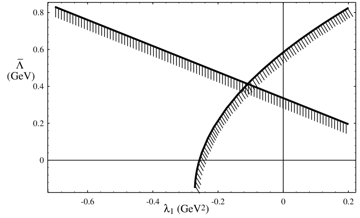
FIG. 4.: Correlated one-loop limits on $\bar{\Lambda}$ and $\lambda_{1}$. The shaded region is ruled out by our analysis of the first two moments of $(s_{H}-\bar{m}_{D}^{2})$.

By this method, we obtain the lower bound

$$\bar{\Lambda}>410\,{\rm MeV}\,,$$ (101)

independent of $\lambda_{1}$. Where the bound on $\bar{\Lambda}$ is saturated, $\lambda_{1}=-0.11\,{\rm GeV}^{2}$. Our result implies the upper limit $m_{b}^{\rm pole}<4.89\,{\rm GeV}$, without any assumption on $\lambda_{1}$ being made.

This approach complements the recent proposal [26] that $\bar{\Lambda}$ and $\lambda_{1}$ be extracted from moments of the photon energy spectrum in the rare process $B\to X_{s}\gamma$.

VI Higher Loops

In order to apply our results consistently, it is important to know the scale at which to evaluate $\alpha_{s}(\mu)$ in the radiative corrections. It has been shown recently [27] that the naïve choice $\mu=m_{b}$ significantly underestimates the size of the two-loop effects. In particular, the prescription of Brodsky, Lepage and Mackenzie (BLM) [14] suggests that the relevant scale for the radiative corrections in $B\rightarrow X_{u}e\bar{\nu}$ decay is $\mu\sim 0.07\,m_{b}$, when expressed in terms of the $b$ quark pole mass, indicating that two-loop effects are substantial.

It has also been stressed, however, that the BLM prescription may give a misleadingly low scale when relating unphysical quantities [28, 29]. In particular, $\bar{\Lambda}$ is related to the pole mass of the heavy quark, which is not an observable, and in fact suffers from an inherent ambiguity in its definition [24]. In this section, we show that although the BLM prescription indicates that radiative corrections to the first two moments of the invariant mass spectrum for semileptonic $b\to u$ decay are uncontrolled when expressed in terms of the HQET parameter $\bar{\Lambda}$, they are well behaved when expressed in terms of physical quantities.

The portion of the two loop correction to Eq. (73) which is proportional to the QCD evolution parameter $\beta_{0}$ may be determined from the one loop correction, calculated with a massive gluon in the final state, using the techniques of Ref. [30]. Some of the details of the computation are given in Appendix B; we find, for $\hat{m}_{q}=0$,

$${1\over m_{B}^{2}}\langle s_{H}\rangle = {91\over 450}{\alpha_{s}(m_{b})\over\pi}+\left({53\over 180}\pi^{2}-{276043\over 108000}\right)\beta_{0}\left({\alpha_{s}(m_{b})\over\pi}\right)^{2}+{7\over 10}{\bar{\Lambda}\over m_{B}}+\dots$$ (102)

$$\simeq 0.20{\alpha_{s}(m_{b})\over\pi}+3.15\left({\alpha_{s}(m_{b})\over\pi}\right)^{2}+{7\over 10}{\bar{\Lambda}\over m_{B}}+\dots$$ (103)

$$\simeq 0.013+0.013+{7\over 10}{\bar{\Lambda}\over m_{B}}+\dots\,,$$ (104)

where $\beta_{0}=11-2n_{f}/3$ and in the last line we have taken $\alpha_{s}(m_{b})\simeq 0.2$. Clearly the perturbation expansion is poorly controlled. In the BLM scale-setting prescription, the scale $\mu_{\rm BLM}$ of the coupling is chosen such that the two-loop contribution proportional to $\beta_{0}$ is absorbed into the one-loop correction. The poor convergence of the series is reflected in the low BLM scale for this process:

$$\mu_{\rm BLM}=m_{b}\exp\left[-2\left({53\over 180}\pi^{2}-{276043\over 108000}\right)/{91\over 450}\right]\simeq 0.03m_{b}\simeq 140\,{\rm MeV}\,.$$ (105)

However, our expression for $\langle s_{H}\rangle$ is given in terms of the unphysical parameter $\bar{\Lambda}$. While this is perfectly acceptable as an intermediate step, since we are ultimately interested only in relations between observable quantities, it has the effect of making the perturbative expansion appear ill-behaved. Instead, let us define the “decay mass” of the $b$ quark, ${m_{b}^{\Gamma}}$, via the charmless semileptonic partial width of the $B$ meson,

$$\Gamma(B\rightarrow X_{u}e\bar{\nu}_{e})\equiv{G_{F}^{2}|V_{ub}|^{2}\over 192\pi^{3}}({m_{b}^{\Gamma}})^{5}.$$ (106)

The decay mass ${m_{b}^{\Gamma}}$ is a physical observable and is therefore well-defined. It is related to the pole mass via the expansion

$${m_{b}^{\Gamma}}=m_{b}^{\rm pole}\left[1+\left({5\over 6}-{2\over 15}\pi^{2}\right){\alpha_{s}(m_{b})\over\pi}-(0.596\beta_{0}+c)\left({\alpha_{s}(m_{b})\over\pi}\right)^{2}+\dots+{\lambda_{1}-9\lambda_{2}\over 10m_{b}^{2}}+\dots\right]\,.$$ (107)

The two-loop term proportional to $\beta_{0}$, which one expects to dominate the two loop result, was calculated in Ref. [27]. The constant $c$ has not been computed. Since $m_{b}^{\rm pole}$ is not well-defined due to renormalon effects, the perturbation series in Eq. (107) has a renormalon ambiguity at ${\cal O}(1/m_{b})$.

Defining a physical version of the parameter $\bar{\Lambda}$,

$$\bar{\Lambda}_{b}^{\Gamma}\equiv m_{B}-{m_{b}^{\Gamma}}\,,$$ (108)

we have

$${\bar{\Lambda}\over m_{B}}={\bar{\Lambda}_{b}^{\Gamma}\over m_{B}}+\left({5\over 6}-{2\over 15}\pi^{2}\right){\alpha_{s}(m_{b})\over\pi}-(0.596\beta_{0}+c)\left({\alpha_{s}(m_{b})\over\pi}\right)^{2}+{\cal O}(\alpha_{s}^{3},1/m_{b}^{2})\,,$$ (109)

and Eq. (102) becomes

$${1\over m_{B}^{2}}\langle\hat{s}_{H}\rangle \simeq (0.202-0.337){\alpha_{s}(m_{b})\over\pi}+(3.151-3.752)\left({\alpha_{s}(m_{b})\over\pi}\right)^{2}+{7\over 10}{\bar{\Lambda}_{b}^{\Gamma}\over m_{B}}$$ (110)

$$\simeq -0.135{\alpha_{s}(m_{b})\over\pi}-0.601\left({\alpha_{s}(m_{b})\over\pi}\right)^{2}+{7\over 10}{\bar{\Lambda}_{b}^{\Gamma}\over m_{B}}$$ (111)

$$\simeq -0.0086-0.0024+{7\over 10}{\bar{\Lambda}_{b}^{\Gamma}\over m_{B}}\,.$$ (112)

The perturbation expansion clearly has improved dramatically. The corresponding BLM scale is now

$$\mu_{\rm BLM}=m_{b}\exp\left[-(2/9)0.601/0.135\right]\simeq 0.37\,m_{b}\,,$$ (113)

which is significantly greater than before.

It is interesting to note that the cancellation we observe in Eq. (110) persists at higher orders in the bubble sum. Using the techniques of Ref. [31] we can calculate the $n$ loop bubble graph, from which we may extract the coefficient of $\beta_{0}^{n}\alpha_{s}^{n+1}$ in the perturbative expansion for $\langle\hat{s}_{0}\rangle$. Although there is no reason to believe that this is the dominant contribution at this order, since there is no $\beta_{0}\rightarrow\infty$ limit of QCD in which the quark and gluon bubble graphs dominate, it does give one class of contributions to the $n$ loop graphs which displays a factorial divergence at large orders in perturbation theory.

Using the techniques of Ref. [31], the perturbation series in Eq. (102) continues as

$${1\over m_{B}^{2}}\langle\hat{s}_{H}\rangle = 0.202{\alpha_{s}(m_{b})\over\pi}+3.151\left({\alpha_{s}(m_{b})\over\pi}\right)^{2}+51.91\left({\alpha_{s}(m_{b})\over\pi}\right)^{3}$$ (115)

$$+940.52\left({\alpha_{s}(m_{b})\over\pi}\right)^{4}+19347.5\left({\alpha_{s}(m_{b})\over\pi}\right)^{5}+{7\over 10}{\bar{\Lambda}\over m_{B}}+\dots\,,$$

and using the results of Ref. [29] for the higher order relation between $m_{b}$ and ${m_{b}^{\Gamma}}$, Eq. (110) continues as

$${1\over m_{B}^{2}}\langle\hat{s}_{H}\rangle = (0.202-0.337){\alpha_{s}(m_{b})\over\pi}+(3.151-3.752)\left({\alpha_{s}(m_{b})\over\pi}\right)^{2}$$ (118)

$$+(51.91-50.37)\left({\alpha_{s}(m_{b})\over\pi}\right)^{3}+(940.52-782.42)\left({\alpha_{s}(m_{b})\over\pi}\right)^{4}$$

$$+(19347.5-14424.2)\left({\alpha_{s}(m_{b})\over\pi}\right)^{5}+{7\over 10}{\bar{\Lambda}_{b}^{\Gamma}\over m_{B}}+\dots$$

$$= -0.135{\alpha_{s}(m_{b})\over\pi}-0.601\left({\alpha_{s}(m_{b})\over\pi}\right)^{2}+1.56\left({\alpha_{s}(m_{b})\over\pi}\right)^{3}$$ (120)

$$+148.1\left({\alpha_{s}(m_{b})\over\pi}\right)^{4}+4923.\left({\alpha_{s}(m_{b})\over\pi}\right)^{5}+{7\over 10}{\bar{\Lambda}_{b}^{\Gamma}\over m_{B}}+\dots$$

$$\simeq -0.0086-0.0024+0.0004+0.0026+0.0051+{7\over 10}{\bar{\Lambda}_{b}^{\Gamma}\over m_{B}}+\dots$$ (121)

Note that even at higher orders there is significant cancellation between the two series. This is similar to the behaviour observed in a different context in Ref. [29]. The remaining bad behaviour presumably reflects the presence of unphysical parameters (such as $\bar{\Lambda}^{2}$ and $\lambda_{1}$) at higher orders in the operator product expansion. Assuming the series is asymptotic, the size of the smallest term in the expansion gives a measure of the uncertainty in the sum of the series.

We do not find a similar cancellation for the second moment of $s_{H}$. For $\hat{m}_{q}=0$ and to order $1/m_{b}$, we find

$${1\over m_{B}^{4}}\langle s_{H}^{2}\rangle=\langle\hat{s}_{0}^{2}\rangle+4{\bar{\Lambda}\over m_{B}}\left(\langle\hat{E}_{0}\hat{s}_{0}\rangle-\langle\hat{s}_{0}^{2}\rangle\right)+\dots\,.$$ (122)

Since $\langle\hat{E}_{0}\hat{s}_{0}\rangle$ and $\langle\hat{s}_{0}^{2}\rangle$ are both order $\alpha_{s}$, there is no $\beta_{0}\alpha_{s}^{2}$ term introduced by expressing $\langle s_{H}^{2}\rangle$ in terms of $\bar{\Lambda}_{b}^{\Gamma}$. However, the naïve counting of powers of $\beta_{0}$ does not work here, because $\langle\hat{s}_{0}^{2}\rangle\ll\langle\hat{E}_{0}\hat{s}_{0}\rangle,\langle\hat{s}_{0}\rangle$. Instead, the ${\cal O}(\beta_{0}\alpha_{s}^{2})$ correction to $\langle\hat{s}_{0}^{2}\rangle$ is the same order as the ${\cal O}(\alpha_{s}^{2})$ term introduced by expressing $\langle s_{H}^{2}\rangle$ in terms of $\bar{\Lambda}_{b}^{\Gamma}$. Using the $\beta_{0}\alpha_{s}^{2}$ term as an estimate of the full two loop correction to $\langle s_{0}^{2}\rangle$ alone, we find, using the same technique as before,

$$\langle s_{0}^{2}\rangle={5\over 324}{\alpha_{s}(m_{b})\over\pi}+\left({277\over 648}\pi^{2}-{25511\over 6075}\right)\beta_{0}\left({\alpha_{s}(m_{b})\over\pi}\right)^{2}+\dots\,,$$ (123)

and so

$${1\over m_{B}^{4}}\langle s_{H}^{2}\rangle = 0.015{\alpha_{s}(m_{b})\over\pi}+0.0196\beta_{0}\left({\alpha_{s}(m_{b})\over\pi}\right)^{2}+0.298\left({\bar{\Lambda}_{b}^{\Gamma}\over m_{B}}-0.48{\alpha_{s}(m_{b})\over\pi}\right){\alpha_{s}(m_{b})\over\pi}$$ (125)

$$\qquad\mbox{}+0.533\left({\bar{\Lambda}_{b}^{\Gamma}\over m_{B}}-0.48{\alpha_{s}(m_{b})\over\pi}\right)^{2}+\ldots$$

$$= 0.015{\alpha_{s}(m_{b})\over\pi}+0.156\left({\alpha_{s}(m_{b})\over\pi}\right)^{2}-0.214{\bar{\Lambda}_{b}^{\Gamma}\over m_{B}}{\alpha_{s}(m_{b})\over\pi}+\dots$$ (126)

$$\simeq 9.5\times 10^{-4}+6.3\times 10^{-4}-0.214{\bar{\Lambda}_{b}^{\Gamma}\over m_{B}}{\alpha_{s}(m_{b})\over\pi}+\dots\,.$$ (127)

The contribution of the $\beta_{0}\alpha_{s}^{2}$ term to this expression is $7.1\times 10^{-4}$, and the new ${\cal O}(\alpha_{s}^{2})$ terms, while of the same order as this one, largely cancel against each other. Since the convergence of the perturbation series for $\langle s_{H}^{2}\rangle$ still appears to be poor, we may also expect the limits on $\bar{\Lambda}$ and $\lambda_{1}$ which we obtained from $\langle(s_{H}-\bar{m}_{D}^{2})^{2}\rangle$ to be more sensitive to higher order perturbative corrections than those obtained from $\langle s_{H}-\bar{m}_{D}^{2}\rangle$.

Finally, note that the appearance of $\bar{\Lambda}$ in $\langle s_{H}^{2}\rangle$ is suppressed by a factor of $\alpha_{s}$, as is its associated renormalon at ${\cal O}(1/m_{b})$. Since renormalon ambiguities must cancel in relations between physical quantities, this means that the large $\beta_{0}\alpha_{s}^{2}$ term in $\langle s_{H}^{2}\rangle$ does not correspond to a ${\cal O}(1/m_{b})$ renormalon ambiguity in the perturbation series (123).

VII Summary and Conclusions

We have used the operator product expansion and the heavy quark limit to compute the hadronic energy and invariant mass spectra in semileptonic heavy meson decays. Our expressions are complete up to order $\alpha_{s}$ in perturbation theory, and up to order $\alpha_{s}/m_{b}$ and $1/m_{b}^{2}$ in the heavy quark expansion. The effects of finite final state quark masses have been taken into account, so it is possible to apply our results to the important decay $b\to c\,\ell\nu$.

Our analysis provides a test of the applicability of the OPE to these decays, and of the crucial underlying concept of global duality. Only appropriately weighted integrals of the theoretical spectra may be compared meaningfully with experiment, and we focus on the leading moments. As an initial application, we used the recent measurement of the $B$ branching fraction to excited $D$ mesons to put bounds on the nonperturbative parameters $\bar{\Lambda}$ and $\lambda_{1}$. We found $\bar{\Lambda}>410\,$MeV, which led to a constraint on the $b$ quark pole mass, $m_{b}^{\rm pole}<4.89\,{\rm GeV}$. More stringent tests will have to await the availability of more precise data. The success or failure of our predictions will determine the confidence with which one will trust these theoretical techniques in the extraction of CKM matrix elements from semileptonic bottom and charm decays.

We also investigated the behaviour of the perturbation series at higher order in $\alpha_{s}$, to gain insight into the trustworthiness of the lowest order calculation and the choice of renormalization scale $\mu$. We found that when written in terms of the unphysical quantity $\bar{\Lambda}$, the perturbation series for $\langle s_{H}\rangle$ seems to be quite badly behaved, with a BLM scale $\mu_{{\rm BLM}}$ too low to be meaningful. However, when we define a more physical “decay mass” $m_{b}^{\Gamma}$, and through it a physical $\bar{\Lambda}_{b}^{\Gamma}$, the perturbation series improves dramatically. The cancellations which we find persist to higher order in $\alpha_{s}$, at least when one includes the leading powers of $\beta_{0}$.

We have focused on the application to $B$ decays; however, the BLM analysis suggests that the perturbative corrections to $\langle s_{H}\rangle$ are under control for $D$ decays as well. The extension of our results to charm is straightforward.

A The parton level hadronic energy spectrum

In this appendix we discuss the corrections to the parton level hadronic energy spectrum, ${\rm d}\Gamma_{0}/{\rm d}\hat{E}_{0}$. Both the perturbative and the power corrections are somewhat unwieldy; we present them here for completeness.

The power correction may be computed by integrating the doubly differential spectrum (15) over $\hat{s}_{0}$. The integral will be nonzero only if $\hat{E}_{0}\leq{1\over 2}(1+\hat{m}_{q}^{2})$, because, as discussed in Section II, only in this case does the integration region overlap with the one-particle pole at $\hat{s}_{0}=\hat{m}_{q}^{2}$. This is a reflection of the fact that the maximum energy a single quark can carry away from the decay is ${1\over 2}(1+\hat{m}_{q}^{2})$. In the presence of additional strongly interacting particles such as gluons, the total hadronic energy $\hat{E}_{0}$ can exceed ${1\over 2}(1+\hat{m}_{q}^{2})$.

However, the initial motion of the $b$ quark inside the $B$ meson can produce fluctuations of the maximum allowed final quark energy above ${1\over 2}(1+\hat{m}_{q}^{2})$. These fluctuations appear in the differential rate as singular functions $\delta(\hat{E}_{0}-{1\over 2}(1+\hat{m}_{q}^{2}))$ and $\delta^{\prime}(\hat{E}_{0}-{1\over 2}(1+\hat{m}_{q}^{2}))$, which are resummed into a smooth function extending beyond the parton model endpoint. For a more detailed discussion of this subject see Refs. [4, 17, 18].

Including the leading power corrections, then, the expression for the hadronic energy spectrum is given by

$${1\over\Gamma_{0}}{{\rm d}\Gamma\over{\rm d}\hat{E}_{0}} = 16\sqrt{\hat{E}_{0}^{2}-\hat{m}_{q}^{2}}\left[3\hat{E}_{0}-4\hat{E}_{0}^{2}-2\hat{m}_{q}^{2}+3\hat{E}_{0}\hat{m}_{q}^{2}\right]$$ (A5)

$$+{16\over\sqrt{\hat{E}_{0}^{2}-\hat{m}_{q}^{2}}}\left[{\lambda_{1}\over 2m_{b}^{2}}\left(-6\hat{E}_{0}^{2}+12\hat{E}_{0}^{3}+{20\over 3}\hat{E}_{0}^{4}+3\hat{m}_{q}^{2}-6\hat{E}_{0}\hat{m}_{q}^{2}-{52\over 3}\hat{E}_{0}^{2}\hat{m}_{q}^{2}+{23\over 3}\hat{m}_{q}^{4}\right)\right.$$

$$\qquad\left.+{\lambda_{2}\over 2m_{b}^{2}}\left(-3\hat{E}_{0}-6\hat{E}_{0}^{2}+36\hat{E}_{0}^{3}+20\hat{E}_{0}^{4}+3\hat{m}_{q}^{2}-21\hat{E}_{0}\hat{m}_{q}^{2}-52\hat{E}_{0}^{2}\hat{m}_{q}^{2}+23\hat{m}_{q}^{4}\right)\right]$$

$$+(1-\hat{m}_{q}^{2})^{3}\,\left[\displaystyle{\lambda_{1}\over 3m_{b}^{2}}(5-\hat{m}_{q}^{2})-\displaystyle{\lambda_{2}\over m_{b}^{2}}(1-5\hat{m}_{q}^{2})\right]\ \delta\left(\hat{E}_{0}-{1\over 2}(1+\hat{m}_{q}^{2})\right)\,$$

$$+\displaystyle{\lambda_{1}\over 6m_{b}^{2}}(1-\hat{m}_{q}^{2})^{5}\ \delta^{\prime}\left(\hat{E}_{0}-{1\over 2}(1+\hat{m}_{q}^{2})\right)+{\cal O}(\alpha_{s},1/m_{b}^{3})\,.$$

Integrating this expression with respect to $\hat{E}_{0}$, we find the power corrections (47) to the moments $\langle\hat{E}_{0}\rangle$ and $\langle\hat{E}_{0}^{2}\rangle$.

The expression for the perturbative correction to the hadronic energy spectrum is even more cumbersome. For the complete spectrum at finite $\hat{m}_{q}$, we refer the reader to Ref. [13]. As an illustration we present here the perturbative corrections at $\hat{m}_{q}=0$, separately for $\hat{E}_{0}<{1\over 2}$ and $\hat{E}_{0}>{1\over 2}$:

$$\left.{1\over\Gamma_{0}}{{\rm d}\Gamma\over{\rm d}\hat{E}_{0}}\right|_{0<\hat{E}_{0}<{1\over 2}}^{\rm pert.} = {\alpha_{s}\over\pi}\,E_{0}^{2}\bigg{[}36-{32\over 3}\pi^{2}-{496\over 9}\hat{E}_{0}+{128\over 9}\pi^{2}\hat{E}_{0}+{52\over 3}\hat{E}_{0}^{2}-{112\over 45}\hat{E}_{0}^{3}+{64\over 135}\hat{E}_{0}^{4}$$ (A8)

$$\qquad\qquad-24\ln(2\hat{E}_{0})+{64\over 3}\hat{E}_{0}\ln(2\hat{E}_{0})+16\ln(2\hat{E}_{0})\ln(1-2\hat{E}_{0})$$

$$\qquad\qquad-{64\over 3}\hat{E}_{0}\ln(2\hat{E}_{0})\ln(1-2\hat{E}_{0})+16{\rm Li}_{2}(2\hat{E}_{0})-{64\over 3}\hat{E}_{0}{\rm Li}_{2}(2\hat{E}_{0})\bigg{]}\,,$$

$$\left.{1\over\Gamma_{0}}{{\rm d}\Gamma\over{\rm d}\hat{E}_{0}}\right|_{{1\over 2}<\hat{E}_{0}<1}^{\rm pert.} = {\alpha_{s}\over\pi}\Bigg{[}{208\over 45}+{1058\over 45}\hat{E}_{0}-{646\over 9}\hat{E}_{0}^{2}+{1592\over 27}\hat{E}_{0}^{3}-{52\over 3}\hat{E}_{0}^{4}+{112\over 45}\hat{E}_{0}^{5}-{64\over 135}\hat{E}_{0}^{6}$$ (A14)

$$\qquad+{5\over 9}\ln(2\hat{E}_{0}-1)+{8\over 3}\hat{E}_{0}\ln(2\hat{E}_{0}-1)+{16\over 3}\hat{E}_{0}^{2}\ln(2\hat{E}_{0}-1)$$

$$\qquad-{64\over 9}\hat{E}_{0}^{3}\ln(2\hat{E}_{0}-1)+8\hat{E}_{0}^{2}\ln^{2}(2\hat{E}_{0}-1)-{32\over 3}\hat{E}_{0}^{3}\ln^{2}(2\hat{E}_{0}-1)$$

$$\qquad-16\hat{E}_{0}^{2}\ln(2\hat{E}_{0})\ln(2\hat{E}_{0}-1)+{64\over 3}\hat{E}_{0}^{3}\ln(2\hat{E}_{0})\ln(2\hat{E}_{0}-1)$$

$$\qquad-16\hat{E}_{0}^{2}{\rm Li}_{2}\left({1\over 2\hat{E}_{0}}\right)+{64\over 3}\hat{E}_{0}^{3}{\rm Li}_{2}\left({1\over 2\hat{E}_{0}}\right)+16\hat{E}_{0}^{2}{\rm Li}_{2}\left({2\hat{E}_{0}-1\over 2\hat{E}_{0}}\right)$$

$$\qquad-{64\over 3}\hat{E}_{0}^{3}{\rm Li}_{2}\left({2\hat{E}_{0}-1\over 2\hat{E}_{0}}\right)\Bigg{]}\,.$$

This spectrum is shown in Fig. 5. The logarithmic divergence as $\hat{E}_{0}\to{1\over 2}$ from above is integrable. The region $\hat{E}_{0}>\frac{1}{/}2$ receives contributions only from brehmsstrahlung graphs. Note that the spectrum falls extremely rapidly with increasing $\hat{E}_{0}$.

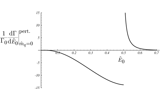
FIG. 5.: The order $\alpha_{s}$ contribution to the differential energy spectrum $(1/\Gamma_{0}){\rm d}\Gamma/{\rm d}\hat{E}_{0}$, for $\hat{m}_{q}=0$, in units of $\alpha_{s}/\pi$. In the region $\hat{E}_{0}>{1\over 2}$, this is the leading nonzero contribution. The logarithmic divergence at $\hat{E}_{0}={1\over 2}$ is integrable.

The radiative corrections $A_{m}(\hat{m}_{q})$ to the moments $\langle\hat{E}_{0}^{m}\rangle$ may be obtained by integrating the full expressions found in Ref. [13]. We find

$$A_{0}(\hat{m}_{q})= {25\over 6}-{2\over 3}\pi^{2}-{478\over 9}\hat{m}_{q}^{2}+{64\over 3}\pi^{2}(1+\hat{m}_{q}^{2})\hat{m}_{q}^{3}-{32\over 3}\pi^{2}\hat{m}_{q}^{4}+{478\over 9}\hat{m}_{q}^{6}$$ (A21)

$$-\left({25\over 6}+{2\over 3}\pi^{2}\right)\hat{m}_{q}^{8}-{2\over 3}(36+\hat{m}_{q}^{4})\hat{m}_{q}^{4}\ln^{2}\hat{m}_{q}^{2}$$

$$+\left(-{40\over 3}\hat{m}_{q}^{2}+{256\over 3}(1+\hat{m}_{q}^{2})\ln(1+\hat{m}_{q})\hat{m}_{q}^{3}-60\hat{m}_{q}^{4}+{8\over 9}\hat{m}_{q}^{6}-{34\over 9}\hat{m}_{q}^{8}\right)\ln\hat{m}_{q}^{2}$$

$$+\left(-{34\over 9}+{128\over 9}\hat{m}_{q}^{2}-{128\over 9}\hat{m}_{q}^{6}+{34\over 9}\hat{m}_{q}^{8}\right)\ln(1-\hat{m}_{q}^{2})$$

$$+\left({8\over 3}-{128\over 3}(1+\hat{m}_{q}^{2})\hat{m}_{q}^{3}+80\hat{m}_{q}^{4}+{8\over 3}\hat{m}_{q}^{8}\right)\ln\hat{m}_{q}^{2}\ln(1-\hat{m}_{q}^{2})$$

$$+\left(4+{128\over 3}(1+\hat{m}_{q}^{2})\hat{m}_{q}^{3}+64\hat{m}_{q}^{4}+4\hat{m}_{q}^{8}\right){\rm Li}_{2}(\hat{m}_{q}^{2})$$

$$-{512\over 3}\hat{m}_{q}^{3}(1+\hat{m}_{q}^{2}){\rm Li}_{2}(\hat{m}_{q})\,,$$

$$A_{1}(\hat{m}_{q})= {1381\over 900}-{7\over 30}\pi^{2}-\left({3133\over 900}+{5\over 18}\pi^{2}\right)\hat{m}_{q}^{2}+\left({99329\over 1350}+{16\over 3}\pi^{2}\right)\hat{m}_{q}^{4}-{1408\over 45}\pi^{2}\hat{m}_{q}^{5}$$ (A29)

$$-\left({100729\over 1350}-{16\over 3}\pi^{2}\right)\hat{m}_{q}^{6}+\left({4933\over 900}-{5\over 18}\pi^{2}\right)\hat{m}_{q}^{8}-\left({6743\over 2700}+{7\over 30}\pi^{2}\right)\hat{m}_{q}^{10}$$

$$+\left(6\hat{m}_{q}^{4}+{34\over 3}\hat{m}_{q}^{6}-{5\over 18}\hat{m}_{q}^{8}-{7\over 30}\hat{m}_{q}^{10}\right)\ln^{2}\hat{m}_{q}^{2}$$

$$+\left(-{47\over 30}\hat{m}_{q}^{2}+{1651\over 45}\hat{m}_{q}^{4}-{5632\over 45}\ln(1+\hat{m}_{q})\hat{m}_{q}^{5}+{1391\over 45}\hat{m}_{q}^{6}+{121\over 135}\hat{m}_{q}^{8}-{409\over 450}\hat{m}_{q}^{10}\right)\ln\hat{m}_{q}^{2}$$

$$+\left(-{61\over 50}+{97\over 54}\hat{m}_{q}^{2}-4\hat{m}_{q}^{4}+4\hat{m}_{q}^{6}-{97\over 54}\hat{m}_{q}^{8}+{61\over 50}\hat{m}_{q}^{10}\right)\ln(1-\hat{m}_{q}^{2})$$

$$+\left({14\over 15}+{10\over 9}\hat{m}_{q}^{2}-{100\over 3}\hat{m}_{q}^{4}+{2816\over 45}\hat{m}_{q}^{5}-{100\over 3}\hat{m}_{q}^{6}+{10\over 9}\hat{m}_{q}^{8}+{14\over 15}\hat{m}_{q}^{10}\right)\ln\hat{m}_{q}^{2}\ln(1-\hat{m}_{q}^{2})$$

$$+\left({7\over 5}+{5\over 3}\hat{m}_{q}^{2}-32\hat{m}_{q}^{4}-{2816\over 45}\hat{m}_{q}^{5}-32\hat{m}_{q}^{6}+{5\over 3}\hat{m}_{q}^{8}+{7\over 5}\hat{m}_{q}^{10}\right){\rm Li}_{2}(\hat{m}_{q}^{2})$$

$$+{11264\over 45}\hat{m}_{q}^{5}\,{\rm Li}_{2}(\hat{m}_{q})\,,$$

and

$$A_{2}(\hat{m}_{q})= {2257\over 3600}-{4\over 45}\pi^{2}+\left({2929\over 5400}-{1\over 5}\pi^{2}\right)\hat{m}_{q}^{2}-{324727\over 10800}\hat{m}_{q}^{4}+{64\over 5}\pi^{2}(1+\hat{m}_{q}^{2})\hat{m}_{q}^{5}$$ (A38)

$$+\left({173\over 162}-{208\over 27}\pi^{2}\right)\hat{m}_{q}^{6}+{304877\over 10800}\hat{m}_{q}^{8}+\left({1297\over 1800}-{1\over 5}\pi^{2}\right)\hat{m}_{q}^{10}$$

$$-\left({36283\over 32400}+{4\over 45}\pi^{2}\right)\hat{m}_{q}^{12}-\left({116\over 9}\hat{m}_{q}^{6}+{1\over 5}\hat{m}_{q}^{10}+{4\over 45}\hat{m}_{q}^{12}\right)\ln^{2}\hat{m}_{q}^{2}$$

$$+\left(-{2\over 45}\hat{m}_{q}^{2}-{131\over 20}\hat{m}_{q}^{4}+{256\over 5}(1+\hat{m}_{q}^{2})\ln(1+\hat{m}_{q})\hat{m}_{q}^{5}-{5467\over 135}\hat{m}_{q}^{6}-{829\over 180}\hat{m}_{q}^{8}\right.$$

$$\left.\qquad+{23\over 450}\hat{m}_{q}^{10}-{173\over 675}\hat{m}_{q}^{12}\right)\ln\hat{m}_{q}^{2}$$

$$+\left(-{298\over 675}+{1\over 25}\hat{m}_{q}^{2}+2\hat{m}_{q}^{4}-2\hat{m}_{q}^{8}-{1\over 25}\hat{m}_{q}^{10}+{298\over 675}\hat{m}_{q}^{12}\right)\ln(1-\hat{m}_{q}^{2})$$

$$+\left({16\over 45}+{4\over 5}\hat{m}_{q}^{2}-{128\over 5}(1+\hat{m}_{q}^{2})\hat{m}_{q}^{5}+{440\over 9}\hat{m}_{q}^{6}+{4\over 5}\hat{m}_{q}^{10}+{16\over 45}\hat{m}_{q}^{12}\right)\ln\hat{m}_{q}^{2}\ln(1-\hat{m}_{q}^{2})$$

$$+\left({8\over 15}+{6\over 5}\hat{m}_{q}^{2}+{128\over 5}(1+\hat{m}_{q}^{2})\hat{m}_{q}^{5}+{416\over 9}\hat{m}_{q}^{6}+{6\over 5}\hat{m}_{q}^{10}+{8\over 15}\hat{m}_{q}^{12}\right){\rm Li}_{2}(\hat{m}_{q}^{2})$$

$$-{512\over 5}(1+\hat{m}_{q}^{2})\hat{m}_{q}^{5}\,{\rm Li}_{2}(\hat{m}_{q})\,.$$

The correction $A_{0}(\hat{m}_{q})$ to the total rate is equivalent to the result presented in Ref. [19].

B Bubble Graphs

The $n$-loop bubble graph contribution to moments of $\hat{s}_{0}$ may be calculated from the one loop graph evaluated with a finite gluon mass [30, 31]. In this appendix, we briefly outline this calculation using the methods of Ref. [31]. Only the bremmstrahlung graphs in Fig. 3 contribute to the moments of $\hat{s}_{0}$ for $n\geq 1$. We consider the expansion

$${{\rm d}\Gamma\over{\rm d}\hat{s}_{0}}=\sum_{j=0}^{\infty}d_{j}(\hat{s}_{0})\beta_{0}^{j}\left({\alpha_{s}\over\pi}\right)^{j+1}+\dots\,,$$ (B1)

where $\beta_{0}=11-2n_{f}/3$ and the ellipses denote terms which have fewer powers of $\beta_{0}\alpha_{s}$ and hence are not obtainable from the bubble graphs. Note that these are not suppressed terms in any limit of QCD, although they may be numerically small. The $n^{\rm th}$ moment of $\hat{s}_{0}$ then has the expansion

$${\cal{M}}^{(n,0)}=\sum_{j=0}^{\infty}m^{(n)}_{j}\,\beta_{0}^{j}\left({\alpha_{s}\over\pi}\right)^{j+1}+\ldots\,,$$ (B2)

where

$$m^{(n)}_{j}=\int_{0}^{1}{\rm d}\hat{s}_{0}\,\hat{s}_{0}^{n}\,d_{j}(\hat{s}_{0})\,.$$ (B3)

Define $d_{0}(\hat{s}_{0},\hat{\lambda}^{2})$ and $m^{(n)}_{0}(\hat{\lambda}^{2})$ to be the one-loop corrections calculated with a finite gluon mass $\lambda$, and $\hat{\lambda}\equiv\lambda/m_{b}$. Then

$$m^{(n)}_{0}(\hat{\lambda}^{2})=\int_{\hat{\lambda}^{2}}^{1}{\rm d}\hat{s}_{0}^{n}\,d_{0}(\hat{s}_{0},\hat{\lambda}^{2})\,,$$ (B4)

and we have [31]

$$d_{j}(\hat{s}_{0})=\left.-{1\over 4^{j}}{{\rm d}^{j}\over{\rm d}u^{j}}\right|_{u=0}{\sin(\pi u)\over\pi u}\int_{0}^{\hat{s}_{0}}\left(\hat{\lambda}^{2}e^{C}\right)^{-u}\,{{\rm d}\over{\rm d}\hat{\lambda}^{2}}d_{0}(\hat{s}_{0},\hat{\lambda}^{2})\,,$$ (B5)

where $C$ is a scheme-dependent constant. In the $V$ scheme[14], $C=0$, while in the $\overline{{\rm MS}}$ scheme, $C=-5/3$. Eqn. (B5) may be written in the form

$$d_{j}(\hat{s}_{0})=\sum_{k=0}^{j}\,c_{k}\,J_{k}(\hat{s}_{0})\,,$$ (B6)

where $J_{k}$ is defined by

$$J_{k}(\hat{s}_{0})\equiv\int_{0}^{\hat{s}_{0}}{\rm d}\hat{\lambda}^{2}\,\ln^{k}(\hat{\lambda}^{2})\,{{\rm d}\over{\rm d}\hat{\lambda}^{2}}d_{0}(\hat{s}_{0},\hat{\lambda}^{2})\,.$$ (B7)

.

Taking moments of both sides of Eq. (B6), we have

$$m^{(n)}_{j} = \sum_{k=0}^{j}\,c_{k}\,\int_{0}^{1}{\rm d}\hat{s}_{0}\,\hat{s}_{0}^{n}\int_{0}^{\hat{s}_{0}}{\rm d}\hat{\lambda}^{2}\,\ln^{k}(\hat{\lambda}^{2})\,{{\rm d}\over{\rm d}\hat{\lambda}^{2}}d_{0}(\hat{s}_{0},\hat{\lambda}^{2})$$ (B8)

$$= \sum_{k=0}^{j}\,c_{k}\,\int_{0}^{1}{\rm d}\hat{\lambda}^{2}\,\int_{\hat{\lambda}^{2}}^{1}{\rm d}\hat{s}_{0}\,\hat{s}_{0}^{n}\ln^{k}(\hat{\lambda}^{2})\,{{\rm d}\over{\rm d}\hat{\lambda}^{2}}d_{0}(\hat{s}_{0},\hat{\lambda}^{2})$$ (B9)

$$= \sum_{k=0}^{j}\,c_{k}\,\int_{0}^{1}{\rm d}\hat{\lambda}^{2}\,\ln^{k}(\hat{\lambda}^{2})\,{{\rm d}\over{\rm d}\hat{\lambda}^{2}}m_{0}^{(n)}(\hat{\lambda}^{2})\,,$$ (B10)

where we have used the fact that $d_{0}(\hat{\lambda}^{2},\hat{\lambda}^{2})=0$ to move the $\hat{s}_{0}$ integral to the right of the $\hat{\lambda}^{2}$ derivative.

It is straightforward to derive analytic expressions for the moments $m_{0}^{(n)}(\hat{\lambda}^{2})$ from the graphs in Fig. 3; however the resulting formulas are lengthy and we will not reproduce them here. For $j=1$ the integrals in Eq. (B8) may be performed analytically, giving the ${\cal O}(\alpha^{2}\beta_{0})$ correction to ${\cal M}^{(n,0)}$, while for $j>1$ we performed the integrals numerically to obtain the contribution from higher loops in the bubble sum.

REFERENCES

[1] M. Voloshin and M. Shifman, Sov. J. Nucl. Phys.
41, 120 (1985).
[2] J. Chay, H. Georgi and B. Grinstein, Phys. Lett. B247, 399 (1990).
[3] I.I. Bigi, N.G. Uraltsev and A.I. Vainshtein,
Phys. Lett. B293, 430 (1992);
I.I. Bigi, M. Shifman, N.G. Uraltsev and A.I. Vainshtein,
Phys. Rev. Lett. 71, 496 (1993);
B. Blok, L. Koyrakh, M. Shifman and A.I. Vainshtein, Phys. Rev.
D49, 3356 (1994); Erratum, Phys. Rev. D50, 3572 (1994).
[6] A. Falk, Z. Ligeti, M. Neubert and Y. Nir, Phys. Lett. B326, 145 (1994); Y. Grossman and Z. Ligeti, Phys. Lett. B347, 399
(1995).
[7] I.I. Bigi, N.G. Uraltsev and A.I. Vainshtein, Phys. Lett. B293, 430 (1992); I.I. Bigi, B. Blok, M. Shifman, N.G. Uraltsev and
A.I. Vainshtein, Minnesota Report No. TPI–MINN–92/67–T (1992);
A.F. Falk,
M. Luke and M.J. Savage, Phys. Rev. D49, 3367 (1994);
M. Neubert, Phys. Rev. D49, 4623 (1994).
[8]
M. Shifman, Mod. Phys. Lett. A10, 605 (1995).
[9]
F. Le Diberder and A. Pich, Phys. Lett. B289, 165 (1992).
[10]
J. Alexander, et al. (CLEO Collaboration), “Measurement
of Hadronic Spectral Moments in decays and a
Determination of ”, CLEO-CONF-94-26 (July 1994).
[16] A.F. Falk and M. Neubert, Phys. Rev. D47,
2965 (1993).
[17] M. Neubert, Phys. Rev. D49, 3392
(1994).
[18] A.F. Falk, E. Jenkins, A.V. Manohar and M.B. Wise,
Phys. Rev. D49, 4553
(1994).
[19] Y. Nir, Phys. Lett. B221, 184 (1989).
[20] M.A. Shifman and M.B. Voloshin, Sov. J. Nucl.
Phys. 47, 511 (1988).
[21] Particle Data Group, Phys. Rev. D50, 1173
(1994).
[22] R. Akers et al. (OPAL Collaboration), Z. Phys. C67, 57 (1995).
[23] A. Falk and M. Peskin, Phys. Rev. D49, 3320 (1994).
[24] M. Beneke and V. M. Braun,
Nucl. Phys. B426, 301 (1994);
I. Bigi et al., Phys. Rev. D50, 2234 (1994);
M. Beneke, V. M. Braun and V. I. Zakharov,
Phys. Rev. Lett. 73, 3058 (1994);
M. Luke, A. V. Manohar and M. J. Savage, Phys. Rev. D51, 4924 (1995);
M. Neubert and C. T. Sachrajda, Nucl. Phys. B438, 235
(1995).
[25] I. Bigi, M. Shifman, N. Uraltsev, A. Vainshtein,
Int. J. Mod. Phys. A9, 2467 (1994); Phys. Rev. D52, 196
(1995).
[26] A. Kapustin and Z. Ligeti, Phys. Lett. B355, 318
(1995).
[27] M. Luke, M.J. Savage and M.B. Wise,
Phys. Lett. B343, 329 (1995);
Phys. Lett. B345, 301 (1995).
[28] S. Brodsky, private communication. See also, for example,
N. Uraltsev, TPI-MINN-95-5-T, hep-ph/9503404, March 1995.
[29] P. Ball, M. Beneke and V.M. Braun, Phys. Rev. D52,
3929
(1995).
[30] B.H. Smith and M.B. Voloshin,
Phys. Lett. B340, 176 (1994).
[31] M. Beneke and V.M. Braun, Phys. Lett. B348, 513
(1995);
P. Ball, M. Beneke and V.M. Braun, Nucl. Phys. B452, 563 (1995).