Indirect CP-Violation in the Neutral Kaon System Beyond Leading Logarithms

Abstract

We have calculated the short distance QCD coefficient $\eta_{3}$ of the effective $|\Delta\text{S}|\text{=2}$-hamiltonian in the next-to-leading order of renormalization group improved perturbation theory. Since now all coefficients $\eta_{1}$, $\eta_{2}$ and $\eta_{3}$ are known beyond the leading log approximation, one can achieve a much higher precision in the theoretical analysis of $\varepsilon_{K}$, the parameter of indirect CP-violation in ${\text{ K}^{0}\!-\!\overline{\text{K}^{0}}}\,$-mixing. The measured value for $\varepsilon_{K}$ yields a lower bound on each of $|V_{cb}|$, $|V_{ub}/V_{cb}|$, the top quark mass $m_{t}$ and the non-perturbative parameter $B_{K}$ as a function of the remaining three quantities. E.g. $m_{t}^{\text{pole}}=176\,\text{GeV}$, $|V_{cb}|=0.040$ and $B_{K}=0.75$ implies $|V_{ub}/V_{cb}|\geq 0.0778$, if the measured value for $\varepsilon_{K}$ is attributed solely to Standard Model physics. We further discuss the implications on the CKM phase $\delta$, $\left|V_{td}\right|$ and the key quantity for all CP-violating processes, $\text{Im}\,\lambda_{t}=\text{Im}\,\left[V^{*}_{ts}V_{td}\right]$. These quantities and the improved Wolfenstein parameters $\bar{\rho}$ and $\bar{\eta}$ are tabulated and the shape of the unitarity triangle is discussed. We compare the range for $|V_{td}|$ with the one obtained from the analysis of ${\text{B}_{d}^{0}\!-\!\overline{\text{B}^{0}_{d}}}\,$-mixing. For $0.037\leq\left|V_{cb}\right|\leq 0.043$, $0.06\leq\left|V_{ub}/V_{cb}\right|\leq 0.10$ and $0.65\leq B_{K}\leq 0.85$ we find from a combined analysis of $\varepsilon_{K}$ and the ${\text{B}_{d}^{0}\!-\!\overline{\text{B}^{0}_{d}}}\,$-mixing paramater $x_{d}$: $49^{\circ}\leq\delta\leq 146^{\circ}$, $7.4\cdot 10^{-3}\leq\left|V_{td}\right|\leq 12.4\cdot 10^{-3}$, $0.85\cdot 10^{-4}\leq\text{Im}\,\lambda_{t}\leq 1.60\cdot 10^{-4}$, $-0.36\leq\bar{\rho}\leq 0.28$ and $0.21\leq\bar{\eta}\leq 0.44$. We predict the mass difference of the $B_{s}^{0}$ system to lie in the range $6.5\,ps^{-1}\leq\Delta m_{B_{s}}\leq 28\,ps^{-1}$. Finally we have a 1995 look at the ${\text{K}_{\text{L}}\!-\!\text{K}_{\text{S}}}\,$-mass difference.

I Introduction

Since its discovery in the year 1964 [1] the study of CP-violation is of continuous interest to both experimentalists and theoreticians. The Standard Model mechanism of CP-violation involves only a single parameter, the phase $\delta$ in the Cabibbo-Kobayashi-Maskawa (CKM) matrix. Hence first the investigation of CP-violating processes is a useful tool in the determination of the CKM elements, some of which are poorly known at present. Second it may be the key to find physics beyond the Standard Model, once one will not be able to fit different observables with the single parameter $\delta$.

Yet at present CP-violation is only precisely and unambiguously measured in $|\Delta\text{S}|\text{=2}$-transitions. It manifests itself in the fact that the neutral Kaon mass eigenstates $|\text{K}_{\text{L}}\rangle$ and $|\text{K}_{\text{S}}\rangle$ are no CP eigenstates. This indirect CP-violation is characterized by the parameter

$$\varepsilon_{K} = \frac{\langle(\pi\pi)_{I=0}|H^{|\Delta\text{S}|=1}|\text{K}_{\text{L}}\rangle}{\langle(\pi\pi)_{I=0}|H^{|\Delta\text{S}|=1}|\text{K}_{\text{S}}\rangle}.$$ (1)

Its relation to the low-energy $|\Delta\text{S}|\text{=2}$-hamiltonian $H^{|\Delta\text{S}|=2}$ is given (in the CKM phase convention for $|\text{K}^{0}\rangle$) by

$$\varepsilon_{K} = \frac{e^{i\pi/4}}{\sqrt{2}}\left(\frac{\mbox{Im\,}\langle\text{K}^{0}|H^{|\Delta\text{S}|=2}|\overline{\text{K}^{0}}\rangle}{\Delta m_{K}}+\xi\right).$$ (2)

Here $m_{K}$ is the neutral Kaon mass, $\Delta m_{K}$ is the ${\text{K}_{\text{L}}\!-\!\text{K}_{\text{S}}}\,$-mass difference and $\xi$ is a small quantity related to CP violation in the $|\Delta\text{S}|\!=\!1$ amplitudes, it contributes roughly 3% to $|\varepsilon_{K}|$ (see [2] for details).

The theorist’s challenge is the proper inclusion of the strong interaction, which binds the quarks into hadrons and screens or enhances the CP-violating weak amplitude. Here the short distance QCD effects can be reliably calculated in renormalization group (RG) improved perturbation theory. With our new calculation they are now completely known in the next-to-leading order (NLO). Its phenomenological implications are the subject of this paper, which is organized as follows: In the following section we present the $|\Delta\text{S}|\text{=2}$-hamiltonian in the NLO. The further ingredients of the phenomenological analysis are discussed in sect. III. In sect. IV we analyze which region of the Standard Model parameters is compatible with the observed value for $\varepsilon_{K}$. In sect. V we first determine the CKM phase $\delta$ from $\varepsilon_{K}$. Then we obtain $|V_{td}|$, which is a key quantity for ${\text{B}_{d}^{0}\!-\!\overline{\text{B}^{0}_{d}}}\,$-mixing, and discuss the additional constraints obtained from the measured ${\text{B}_{d}^{0}\!-\!\overline{\text{B}^{0}_{d}}}\,$-mixing mixing parameter $x_{d}$. Further we determine the improved Wolfenstein parameters $\bar{\rho}$ and $\bar{\eta}$ and further $\text{Im}\,\lambda_{t}$, which is proportional to the Jarlskog measure of CP-violation and therefore enters all CP-violating quantities in the Standard Model. Finally we discuss the short distance contributions to the ${\text{K}_{\text{L}}\!-\!\text{K}_{\text{S}}}\,$-mass difference.

II The $|\Delta\text{S}|\text{=2}$-hamiltonian in the next-to-leading order

The low-energy hamiltonian inducing ${\text{ K}^{0}\!-\!\overline{\text{K}^{0}}}\,$-mixing reads:

$$H^{|\Delta S|=2} = \frac{G_{F}^{2}}{16\pi^{2}}M_{W}^{2}\left[\lambda_{c}^{2}\eta_{1}x_{c}\!+\!\lambda_{t}^{2}\eta_{2}S(x_{t})\!+\!2\lambda_{c}\lambda_{t}\eta_{3}S(x_{c},x_{t})\right]b(\mu)Q_{S2}(\mu)+\text{h.c.}\;\;$$ (3)

Here $G_{F}$ is the Fermi constant, $M_{W}$ is the W boson mass and $x_{i}=m_{i}^{2}/M_{W}^{2}$.

$$\lambda_{j}=V_{jd}V_{js}^{*}$$ (4)

comprises the CKM-factors and $Q_{S2}$ is the local four-quark operator

$$Q_{S2} = (\overline{s}_{j}\gamma_{\mu}(1-\gamma_{5})d_{j})(\overline{s}_{k}\gamma^{\mu}(1-\gamma_{5})d_{k})\;=\;(\overline{s}d)_{V-A}(\overline{s}d)_{V-A}$$ (5)

with $j$ and $k$ being colour indices. The Inami-Lim functions [3]

$$S(x_{t}) = x_{t}\left[\frac{1}{4}+\frac{9}{4}\frac{1}{1-x_{t}}-\frac{3}{2}\frac{1}{(1-x_{t})^{2}}\right]-\frac{3}{2}\left[\frac{x_{t}}{1-x_{t}}\right]^{3}\ln x_{t}$$ (6)

$$S(x_{c},x_{t}) = -x_{c}\ln x_{c}+x_{c}\left[\frac{x_{t}^{2}-8x_{t}+4}{4(1-x_{t})^{2}}\ln x_{t}+\frac{3}{4}\frac{x_{t}}{x_{t}-1}\right]$$ (7)

depend on the masses of the charm- and top-quark and describe the $|\Delta\text{S}|\text{=2}$-transition amplitude in the absence of strong interaction.

The short distance QCD corrections are comprised in the coefficients $\eta_{1}$, $\eta_{2}$ and $\eta_{3}$ with a common factor $b(\mu)$ split off. They are functions of the charm and top quark masses and of the QCD scale parameter $\Lambda_{\text{QCD}}$. Further they depend on various renormalization scales. This dependence, however, is artificial, as it originates from the truncation of the perturbation series, and diminishes order-by-order in $\alpha_{s}$. The $\eta_{i}$’s have been calculated in the leading-logarithmic approximation by Gilman and Wise [4] for the case of a light top quark. The corresponding results for a heavy top quark have been derived in [5]. We briefly recall the motivation for the calculation in the NLO:

1. To make use of the fundamental QCD scale parameter $\Lambda_{\overline{\text{MS}}}$ one must calculate beyond the leading order (LO).

2. The quark mass dependence of the $\eta_{i}$’s is not accurately reproduced by the LO expressions. Especially the $m_{t}$-dependent terms in $\eta_{3}\cdot S(x_{c},x_{t})$ belong to the NLO.

3. The LO results for $\eta_{1}$ and $\eta_{3}$ show a large dependence on the renormalization scales, at which one integrates out heavy particles. In the NLO these uncertainties are reduced.

4. One must go to the NLO to judge whether perturbation theory works, i.e. whether the radiative corrections are small. After all the corrections can be sizeable.

In the NLO one has to take care of the proper definition of the quark masses. It is most useful to define the $\eta_{i}$’s with respect to running masses in the $\overline{\text{MS}}$ scheme normalized as $m_{i}^{\star}=m_{i}(m_{i})$. I.e. we use $x_{i}^{\star}=\left[m_{i}(m_{i})\right]^{2}/M_{W}^{2}$ in (3) and mark the corresponding $\eta_{i}$’s with a star. The NLO calculation here requires the use of the one-loop relation between the pole mass and the running mass:

$$m^{\text{pole}} = m^{\star}\left(1+\frac{\alpha_{s}(m^{\star})}{\pi}\frac{4}{3}\right).$$ (8)

The top quark running mass $m_{t}^{\star}$ is smaller than $m_{t}^{\text{pole}}$ by $8\,\text{GeV}$.

$\eta_{2}^{\star}$ and $\eta_{3}^{\star}$ depend very weakly on the charm and top quark mass and on $\Lambda_{\overline{\text{MS}}}^{\text{NLO}}$, so that they can be treated as constants. In contrast $\eta_{1}^{\star}$ is a steep function of $m_{c}^{\star}$ and $\Lambda_{\overline{\text{MS}}}^{\text{NLO}}$.

Now the NLO values read:

$$\eta_{1}^{\star} = 1.32\begin{array}[]{l}\scriptstyle+0.21\\[-1.99168pt] \scriptstyle-0.23\end{array}\,,\quad\quad\eta_{2}^{\star}\;=\;0.57\begin{array}[]{l}\scriptstyle+0.00\\[-1.99168pt] \scriptstyle-0.01\end{array}\,,\quad\quad\eta_{3}^{\star}\;=\;0.47\begin{array}[]{l}\scriptstyle+0.03\\[-1.99168pt] \scriptstyle-0.04\end{array}\,,$$ (15)

where $m_{c}^{\star}=1.3\,\text{GeV}$ and $\Lambda_{\overline{\text{MS}}}^{\text{NLO}}=0.310\,\text{GeV}$ has been used. The quoted theoretical errors are estimated in two ways: First the renormalization scales have been varied and second the calculated $O(\alpha_{s})$–corrections have been squared.

The calculation for $\eta_{1}^{\star}$ has been performed by us [6] and $\eta_{2}^{\star}$ has been obtained by Buras, Jamin and Weisz [7]. The NLO value for $\eta_{3}^{\star}$ in (15) is new. We will present details of the calculation in [8].

For comparison we give the old leading-order central values [4]:

$$\eta_{1}^{\star\,\text{LO}} = 0.80\,,\quad\quad\eta_{2}^{\star\,\text{LO}}\;=\;0.62\,,\quad\quad\eta_{3}^{\star\,\text{LO}}\;=\;0.36\,.$$ (16)

The common factor of the short distance QCD corrections split off in (3) equals

$$b(\mu) = \left[\alpha_{s}(\mu)\right]^{-2/9}\left(1+\frac{307}{162}\frac{\alpha_{s}(\mu)}{4\pi}\right)$$ (17)

in the NLO. Here $\mu$ is the scale at which the perturbative short distance calculation is matched to the non-perturbative evaluation of the hadronic matrix element. The latter must compensate the $\mu$–dependence in (17) and is parametrized by $B_{K}$ as

$$\langle\overline{\text{K}^{0}}|Q_{S2}(\mu)|\text{K}^{0}\rangle = \frac{8}{3}f_{K}^{2}m_{K}^{2}B_{K}/b(\mu).$$ (18)

Here $m_{K}$ and $f_{K}$ are the mass and decay constant of the neutral Kaon.

III Miscellaneous

A CKM Matrix and Unitarity Triangle

For all numerical analyses we will use the exact standard parametrization of the CKM matrix [9]:

$$V\;=\;\left(\begin{array}[]{ccc}V_{ud}&V_{us}&V_{ub}\\ V_{cd}&V_{cs}&V_{cb}\\ V_{td}&V_{ts}&V_{tb}\end{array}\right) = \left(\begin{array}[]{ccc}c_{12}c_{13}&s_{12}c_{13}&s_{13}e^{-i\delta}\\ -s_{12}c_{23}-c_{12}s_{23}s_{13}e^{i\delta}&c_{12}c_{23}-s_{12}s_{23}s_{13}e^{i\delta}&s_{23}c_{13}\\ s_{12}s_{23}-c_{12}c_{23}s_{13}e^{i\delta}&-c_{12}s_{23}-s_{12}c_{23}s_{13}e^{i\delta}&c_{23}c_{13}\end{array}\right)\,,$$ (25)

where $c_{ij}=\cos\theta_{ij}$ and $s_{ij}=\sin\theta_{ij}$.

The unitarity of $V$ provides us with many relations among its elements. The most useful one is

$$V_{ud}V_{ub}^{*}+V_{cd}V_{cb}^{*}+V_{td}V_{tb}^{*} = 0.$$ (26)

With

$$\overline{\rho} = -\text{Re}\,\frac{V_{ud}V_{ub}^{*}}{V_{cd}V_{cb}^{*}},\quad\quad\quad\overline{\eta}\;=\;-\text{Im}\,\frac{V_{ud}V_{ub}^{*}}{V_{cd}V_{cb}^{*}}$$ (27)

(26) describes an unitarity triangle in the complex $\overline{\rho}$–$\overline{\eta}$–plane, whose edges are located at the points $(0,0)$, $(0,1)$ and $(\overline{\rho},\overline{\eta})$ (see fig. 1).

FIG. 1.: The unitarity triangle of (27).

To illustrate the size of the contributions from the different CKM elements we will also use the improved Wolfenstein parametrization [10], which is obtained from (25) by defining the parameters $\lambda,A,\rho$ and $\eta$ by

$$s_{12} = \lambda\;=\;0.22,\quad\quad s_{23}\;=\;A\lambda^{2},\quad\quad s_{13}e^{-i\delta}\;=\;A\lambda^{3}\left(\rho-i\eta\right),$$ (28)

and expanding the cosines in (25) to any desired order in $\lambda=0.22$. The expansion to order $\lambda^{3}$ yields the conventional Wolfenstein parametrization [11]. Yet it is well-known that the proper treatment of CP-violating effects requires a higher accuracy:

$$V = \left(\begin{array}[]{ccc}1-\frac{\lambda^{2}}{2}&\lambda&A\lambda^{3}(\rho-i\eta)\\ -\lambda-iA^{2}\lambda^{5}\eta&1-\frac{\lambda^{2}}{2}&A\lambda^{2}\\ A\lambda^{3}(1-\overline{\rho}-i\overline{\eta})&-A\lambda^{2}-iA\lambda^{4}\eta&1\end{array}\right)$$ (32)

is exact to order $\lambda^{3}$ and contains the phenomenologically important terms up to the order $\lambda^{5}$ [10]. Here $\overline{\rho}$ and $\overline{\eta}$ defined in (27) are expanded as

$$\overline{\rho}\;=\;\rho\left(1-\frac{\lambda^{2}}{2}+O(\lambda^{4})\right), \overline{\eta}\;=\;\eta\left(1-\frac{\lambda^{2}}{2}+O(\lambda^{4})\right).$$ (33)

B CKM Elements from $\varepsilon_{K}$

The experimental value for $|\varepsilon_{K}|$ [9],

$$|\varepsilon_{K}| = (2.266\pm 0.023)\cdot 10^{-3},$$ (34)

constrains the CKM elements with (2), (3) and (18) via

$$1.21\cdot 10^{-7} = B_{K}\left[-\text{Im}\,\lambda_{c}^{2}\,\eta^{\star}_{1}\,S(x^{\star}_{c})-\text{Im}\,\lambda_{t}^{2}\,\eta^{\star}_{2}\,S(x^{\star}_{t})-2\,\text{Im}\,\left(\lambda_{c}\lambda_{t}\right)\,\eta^{\star}_{3}\,S(x^{\star}_{c},x^{\star}_{t})\right].$$ (35)

Here the number on the LHS originates from

$$1.21\cdot 10^{-7} = \frac{12\sqrt{2}\,\pi^{2}\,\Delta m_{K}}{G_{F}^{2}\,F_{K}^{2}\,m_{K}\,M_{W}^{2}}\left(|\varepsilon_{K}|-\frac{\xi}{\sqrt{2}}\right)$$ (36)

with the numerical values for these physical quantities listed in sect. III C. Further $\lambda_{j}$ has been defined in (4) and the small term $\xi$ in (2) has been estimated with the help of [12] to contribute roughly $-3\%$ to $\varepsilon_{K}$. The uncertainty in the LHS due to experimental errors is about 1% and therefore negligible compared to the uncertainties to be discussed in sect. III C.

The relative importance of the three terms in the square bracket in (35) can be demonstrated with the help of the improved Wolfenstein parametrization (32) turning (35) into

$$5.3\cdot 10^{-4} = B_{K}A^{2}\overline{\eta}\left[(1-\overline{\rho})A^{2}\lambda^{4}\eta^{\star}_{2}S(x^{\star}_{t})+\eta^{\star}_{3}S(x^{\star}_{c},x^{\star}_{t})-\eta^{\star}_{1}x^{\star}_{c}\right]$$ (37)

after dividing both sides by $2\,\lambda^{6}$.

In (37) one sees that the top-top contribution is CKM suppressed by four powers of $\lambda$, but this suppression is over-compensated because the top quark is so heavy:

$$\eta^{\star}_{2}S(x^{\star}_{t})\; \approx \;1.3\cdot 10^{3}\cdot\eta^{\star}_{3}S(x^{\star}_{c},x^{\star}_{t})\;\;\approx\;\;4\cdot 10^{3}\cdot\eta^{\star}_{1}x^{\star}_{c}.$$ (38)

Hence $\eta^{\star}_{2}$ is the most important short distance coefficient, $\eta^{\star}_{3}$ is second relevant and $\eta^{\star}_{1}$ contributes least. Their contributions to the RHS of (37) are roughly $75\%$, $37\%$ and $-12\%$. Yet if we look at the changes in the $\eta^{\star}_{i}$’s due to the NLO calculations (cf. (15) and (16)) one realizes that the NLO correction to $\eta^{\star}_{3}$ is the most important one, because it is enhanced by $30\%$, while $\eta^{\star}_{2}$ has decreased by only $8\%$.

C Ranges for the Input Parameters

In this section we will discuss the actual ranges of the input parameters needed for our analysis. To determine $\delta$ from (35) one must first fix the three angles in (25) from the magnitudes of three CKM elements. While $|V_{us}|=0.2205\pm 0.0018$ is well-known [9], the determination of $V_{cb}$ and especially $V_{ub}$ from tree-level b-decays is still plagued by sizeable experimental and theoretical uncertainties. Since these parameters are two main contributors to our final error bars, we will now consider them in more detail:

The theoretical understanding of the determination of $V_{cb}$ from exclusive and inclusive B-decays has recently made significant progress [13]. In [13] presumably large perturbative corrections proportional to $\alpha_{s}^{n+1}\beta_{0}^{n}$ have been summed to all orders in the decay rate resolving both the previous discrepancy between the results of inclusive and exclusive analyses and the large scheme dependence of the inclusive analysis found in [15]. With $\tau_{B_{d}^{0}}=(1.59\pm 0.07)ps$ [16] the result of [13] reads

$$V_{cb} = 0.040\pm 0.003$$ (39)

coinciding with the result presented in [14]. $b\rightarrow u$ decays are harder to treat both theoretically and experimentally. We will use [9]

$$\left|\frac{V_{ub}}{V_{cb}}\right| = 0.08\pm 0.02.$$ (40)

A further ingredient of our analysis is the top quark mass, which has been determined in the CDF experiment [17] to equal

$$m_{t}^{\text{pole}} = (176\pm 13)\,\mbox{GeV}.$$ (41)

In NLO analyses one has to take into account the proper definition of the mass: The corresponding value for the running mass in the $\overline{\text{MS}}$-scheme is

$$m_{t}^{\star}\;=\;m_{t}(m_{t}) = (168\pm 13)\,\mbox{GeV}.$$ (42)

The fit of the top mass from the LEP data yields the same central value with an error bar of roughly the double size [18]. The D0 group finds $m_{t}^{\text{pole}}=(199\pm 30)\,\text{GeV}$ [19]. Yet the analysis in [20] extracting the top mass by partly fitting the cross sections finds a lower value $m_{t}^{\text{pole}}=(170\pm 9)\,\text{GeV}$ from the combined analysis of CDF and D0. Therefore the range given in (42) well represents the possible values for $m_{t}^{\star}$ and will be used in the following sections.

Next we have to discuss the non-perturbative parameter $B_{K}$ defined in (18): The size of $B_{K}$ has been the subject of a controversal discussion during the last decade. The $1/N_{c}$ result $B_{K}=0.7\pm 0.1$ [21] was in contradiction with lower values estimated with chiral symmetry [22] or the QCD hadron duality approach [23]. Yet a recent analysis [24] has vindicated the result of [21] and seems to have explained the difference to the estimates in [22, 23]. Further recent quenched QCD lattice calculations have yielded values around $B_{K}=0.78$ (see [25] and references therein). The effect of dynamical fermions has been found to be small in [26]. We will therefore use the following range in our calculation:

$$B_{K} = 0.75\pm 0.10.$$ (43)

In fact we will see in sect. IV that the inclusion of values lower than $B_{K}=0.65$ can only very hardly be brought into agreement with the measured value of $\varepsilon_{K}$. We remark that the NLO short distance calculation also affects $B_{K}$ because of the factor of $1/b(\mu)$ on the RHS of (18). Non-perturbative calculations determine the matrix element on the LHS of (18) and usually the quoted results for $B_{K}$ are obtained with the leading order factor $b^{\text{LO}}(\mu)=\left[\alpha^{\text{LO}}(\mu)\right]^{-2/9}$ instead of the NLO value given in (17). Hence in a consistent NLO analysis one should correct for this by multiplying the cited values with $b(\mu)/b^{\text{LO}}(\mu)$. Yet numerically this amounts to a change of about $3\%$ for $\mu=O\left(0.7\,\text{GeV}\right)$ and can be neglected in view of the larger uncertainty in (43). But once the lattice results will achieve an accuracy in the percentage region they should be quoted with the NLO factor given in (17).

At this point it is instructive to investigate the impact of our NLO calculation for $\eta_{3}^{\star}$: With (35) one can easily verify that the shift from $\eta_{3}^{\star\,\text{LO}}=0.36$ in (16) to $\eta_{3}^{\star}=0.47$ in (15) has the same influence on $|\varepsilon_{K}|$ as a shift from $B_{K}=0.82$ to $B_{K}=0.75$. In the same way one can estimate the uncertainty caused by the error bar in the NLO values in (15): The remaining uncertainties in the NLO $\eta_{i}^{\star}$’s correspond to a change in $B_{K}$ by $\pm 0.02$.

Let us now look at the other input parameters: The dominant QCD factors $\eta_{2}^{\star}$ and $\eta_{3}^{\star}$ depend very weakly on the QCD scale parameter $\Lambda_{\overline{\text{MS}}}^{\text{NLO}}$, which therefore hardly affects our results for $\varepsilon_{K}$. Yet of course the determination of the input parameters $V_{cb}$ and $|V_{ub}/V_{cb}|$ depends on $\Lambda_{\overline{\text{MS}}}^{\text{NLO}}$; this uncertainty is included in the error bar in (39) and (40) [13]. Conversely the ${\text{K}_{\text{L}}\!-\!\text{K}_{\text{S}}}\,$-mass difference discussed in sect. VI is dominated by $\eta_{1}^{\star}$ which is a steep function of $\Lambda_{\overline{\text{MS}}}^{\text{NLO}}$. We will consider [27]

$$\Lambda_{\overline{\text{MS}}}^{\text{NLO}} = (310\pm 100)\,\text{MeV}$$ (44)

corresponding to

$$\alpha\left(M_{Z}\right) = 0.117\,\pm 0.006.$$ (45)

The situation is the same with respect to the dependence on $m_{c}^{\star}$: The RHS of (35) depends only weakly on $m_{c}^{\star}$. Varying [13]

$$m_{c}^{\star} = (1.29\pm 0.07)\,\text{GeV}$$ (46)

within the quoted range affects the RHS of (35) by $3\%$, i.e. it is negligible compared to the uncertainty in $B_{K}$. Yet the ${\text{K}_{\text{L}}\!-\!\text{K}_{\text{S}}}\,$-mass difference depends on $m_{c}^{\star}$ sizeably.

For completeness we list the remaining parameters entering the analysis of $\varepsilon_{K}$ [9]:

$$G_{F}\;=\;1.17\cdot 10^{-5}\,\text{GeV}^{-2},\quad F_{K}\;=\;161\,\text{MeV},\quad m_{K}\;=\;498\,\text{MeV},$$ (47)

$$\Delta\,m_{K}\;=\;3.52\cdot 10^{-15}\,\text{GeV},\quad M_{W}\;=\;80.22\,\text{GeV},\quad m_{b}^{\star}\;=\;4.2\,\text{GeV}$$ (48)

and the measured value for $|\varepsilon_{K}|$ has been given in (34). The uncertainties of these quantities are irrelevant for the analysis.

Finally we list the additional input parameters needed for the ${\text{ B}^{0}\!-\!\overline{\text{B}^{0}}}\,$-mixing: The ${\text{B}_{d}^{0}\!-\!\overline{\text{B}^{0}_{d}}}\,$-mixing parameter $x_{d}=0.78\pm 0.05$ enters the calculation in the combination

$$\Delta m_{B_{d}} = x_{d}/\tau_{B_{d}}\;=\;(0.496\pm 0.032)\,ps^{-1},$$ (49)

which is the world average presented in [16]. Yet the largest uncertainty is due to the hadronic parameters $F_{B_{d}}$ and $B_{B_{d}}$ appearing in the form

$$F_{B_{d}}\sqrt{B_{B_{d}}} = (195\pm 45)\,\text{MeV}.$$ (50)

This result has been obtained with lattice methods [28] and QCD sum rules [29]. The ratio $F_{B_{s}}/F_{B_{d}}$ has been well determined from the lattice [28]:

$$\frac{F_{B_{s}}}{F_{B_{d}}} = 1.22\pm 0.04.$$ (51)

Further we will need the meson masses $m_{B_{d}}=5.28\,\text{GeV}$ and $m_{B_{s}}=5.38\,\text{GeV}$ and the $B_{s}$ lifetime $\tau_{B_{s}}=(1.53\pm 0.10)\,ps$ [16].

IV Bounds on Standard Model parameters

As explained in the previous section the final error bar of the CKM phase $\delta$ determined from $\varepsilon_{K}$ is due to the uncertainties in $V_{cb}$, $|V_{ub}/V_{cb}|$, $B_{K}$ and $m_{t}^{\star}$. Yet it is well-known that the unitarity of the CKM Matrix constrains the allowed range for these four quantities: If one fixes three of them, a lower bound for the fourth one can be obtained, because otherwise (35) yields no real solutions for $\cos\delta$. In terms of the improved Wolfenstein parameters (32) these solutions appear as the intersection points of a hyperbola with a circle. The lower bound solution corresponds to a set of parameters for which the hyperbola touches the circle in one point (see [10] for details). Prior to the discovery of the top quark this method was used to find a lower bound on the top quark mass (see e.g. [10, 30]). Now in the top era it is more useful to determine the allowed region for the other two fundamental Standard Model parameters in the game, $V_{cb}$ and $|V_{ub}/V_{cb}|$. This is shown in fig. 2. The ranges (39) and (40) correspond to a rectangle in fig. 2. For each pair $(m_{t}^{\star},B_{K})$ the constraint from $\varepsilon_{K}$ defines a curve in fig. 2 such that only the region above this curve is allowed.

FIG. 2.: New physics borderlines for various values of $m_{t}^{\star}$ and $B_{K}$. Each pair $(m_{t}^{\star},B_{K})$ defines a curve. If the Standard Model is the only source of indirect CP violation in the neutral Kaon system, the points below the curve are excluded. The solid line in the middle corresponds to the central values for $m_{t}^{\star}$ and $B_{K}$ given in sect. III C. The rectangle limits the allowed range for $V_{cb}$ and $|V_{ub}/V_{cb}|$ obtained from tree-level b-decays according to (39) and (40). The point in the middle of the rectangle corresponds to the central values in (39) and (40).

We emphasize that the central values for the input parameters given in (39) to (43) are close to the borderline curve depicted in fig. 2. With the old LO value for $\eta_{3}$ the central values would even seem to contradict the measured value for $\varepsilon_{K}$. The minimal value for $|V_{ub}/V_{cb}|$ equals 0.0778, if the central values in (39), (42) and (43) are chosen for the other parameters. Conversely the minimal values for the other parameters read $V_{cb,\,\text{min}}=0.397$, $m^{\star}_{t,\,\text{min}}=164\,\text{GeV}$ and $B_{K,\,\text{min}}=0.729$, if the remaining three ones equal the central values chosen in sect. III C. Of course varying these parameters to higher values relaxes the lower bound on the fourth one. Altogether the constraint from $\varepsilon_{K}$ rules out almost one half of the parameter space of sect. III C.

From these remarks it is clear that $\varepsilon_{K}$ strongly constrains those extensions of the Standard Model, in which extra CP-violating interactions diminish $|\varepsilon_{K}|$, because then the Standard Model contribution $|\varepsilon_{K}^{\text{SM}}|$ must be larger to accommodate for the measured value of $|\varepsilon_{K}|$. The lower bound can be summarized in the following approximate formula

$$\frac{V_{cb}}{0.0397}\,\left(\frac{|V_{ub}/V_{cb}|}{0.080}\right)^{0.27}\left(\frac{m_{t}^{\star}}{168\,\text{GeV}}\right)^{0.31}\left(\frac{B_{K}}{0.75}\right)^{0.27}\left(\frac{2.27\cdot 10^{-3}}{|\varepsilon_{K}^{\text{SM}}|}\right)^{0.27} \geq 1.$$ (52)

$|V_{ub}/V_{cb}|_{\text{min}}$ determined from (52) concides with the exact solution to $4\%$ accuracy in the parameter range of sect. III C. For $0.039\leq V_{cb}\leq 0.041$ the agreement is better than $2\%$.

(52) displays the sensitivity of our analysis on $V_{cb}$. Although $V_{cb}$ is known to a much higher accuracy than $|V_{ub}/V_{cb}|$, its uncertainty contributes roughly as much to the final error as the one of $|V_{ub}/V_{cb}|$. The situation is similar in the analysis of sect. V.

Finally we remark that in the vicinity of the lower bound values the determination of the CKM elements is very sensitive to the input parameters. Because of the required precision one should use the exact parametrization (25) of the CKM matrix here.

V CKM matrix phenomenology

In this section we determine various CKM parameters using $|\varepsilon_{K}|$ and the unitarity of the CKM matrix and discuss the constraints following from ${\text{ B}^{0}\!-\!\overline{\text{B}^{0}}}\,$-mixing.

A The CKM phase $\delta$

By solving eqn. (35) for $\cos\delta$ we calculate the two solutions for the phase $\delta$ of the CKM matrix. For the input parameters defined in sect. III C the resulting $\delta$’s have been compiled into table I, where the dependence on the key parameters $m_{t}^{\star}$, $B_{K}$, $V_{cb}$ and $|V_{ub}/V_{cb}|$ is made explicit. A dash means that there exists no solution for these parameters, lines which do not contain a solution at all have been omitted from the table. This happens for small values of the abovementioned input parameters and served to derive the bounds on these parameters in sect. IV.

For our central values we observe the two solutions being very close to the limits derived in sect. IV. This leads to very asymmetric error bars. Therefore we first give the central values and the variation of it for all relevant parameters separately.

$$\delta^{\text{low}} = 89^{\circ}\begin{array}[]{llll}+13^{\circ}&+13^{\circ}&+13^{\circ}&+13^{\circ}\\ -28^{\circ}&-23^{\circ}&-14^{\circ}&-17^{\circ}\end{array}$$ (55)

$$\delta^{\text{high}} = 116^{\circ}\begin{array}[]{llll}+24^{\circ}&+24^{\circ}&+12^{\circ}&+15^{\circ}\\ -13^{\circ}&-13^{\circ}&-13^{\circ}&-13^{\circ}\end{array}$$ (58)

The variations in (58) are meant as follows: The first number in the lower line for $\delta^{\text{low}}$ and the first number in the upper line for $\delta^{\text{high}}$ are the two solutions obtained by pushing $V_{cb}$ to its maximal value $V_{cb}=0.043$ while keeping the other three parameters fixed to their central values given in sect. III C. Conversely the other three numbers in these lines represent the variation when the same is done for $|V_{ub}/V_{cb}|$, $m_{t}^{\star}$ and $B_{K}$. In contrast moving the key parameters to lower values makes the two solutions for $\delta$ approach until they merge, when the varied parameter reaches its “lower bound value” discussed in the preceding section. The variations on the upper line for $\delta^{\text{low}}$ and the lower line for $\delta^{\text{high}}$ correspond to these values, which are $V_{cb,\text{min}}=0.0397$, $|V_{ub}/V_{cb}|_{\text{min}}=0.0778$, $m^{\star}_{t,\text{min}}=164\,\text{GeV}$ and $B_{K,\text{min}}=0.729$.

We combine the individual variations in (58) to

$$\delta^{\text{low}} = 89^{\circ}{+13^{\circ}\atop-43^{\circ}}$$ (59)

$$\delta^{\text{high}} = 116^{\circ}{+39^{\circ}\atop-13^{\circ}}$$ (60)

The error in the lines stemming from the lower bounds is motivated by the observation that the value $\delta=103^{\circ}$ for which the two solutions merge is essentially independent of the input parameters. The error in the lines emerging from pushing the input parameters to their maximally allowed values is obtained by adding the four individual variations of (58) in quadrature. This seems questionable, because the theoretical errors of the input parameters may be correlated. Hence we have also determined the error by finding simply the maximal value for $\delta^{\text{high}}$ and the minimal value for $\delta^{\text{low}}$ when all input quantities are varied within the ranges given in sect. III C. These extremal values correspond to the point $(V_{cb}=0.043,|V_{ub}/V_{cb}|=0.10,m_{t}^{\star}=181\,\text{GeV},B_{K}=0.85)$, because $\delta^{\text{high}}$ and $\delta^{\text{low}}$ are monotonous functions of all four arguments. This results in an error which is only slightly larger than the one cited in (60), $-48^{\circ}$ instead of $-43^{\circ}$ in $\delta^{\text{low}}$ and $+42^{\circ}$ instead of $+39^{\circ}$ in $\delta^{\text{high}}$. This is caused by the fact that $\delta$ varies only very slowly in the parameter region far away from the central values. $|V_{td}|$ discussed in the following section shows the same behaviour, which is evident from the plots in fig. 3 and fig. 4. Hence the error bars in (60) are clearly not too small.

Let us now remark that in table I the error resulting from the variation of the other parameters entering the calculation is not shown. It amounts to roughly 3–4 degrees.

The discussion of $\delta$ is especially instructive in conjunction with the unitarity triangle. We will therefore return to $\delta$ in sect. V E, where we will also see that the additional incorporation of ${\text{B}_{d}^{0}\!-\!\overline{\text{B}^{0}_{d}}}\,$-mixing yields a tighter upper bound on $\delta$ than the one in (60).

Once we have in this way obtained the phase $\delta$ from the three angles $s_{12}$, $s_{23}$ and $s_{13}$ or equivalently $V_{us}$, $V_{cb}$ and $|V_{ub}/V_{cb}|$, we are by use of (25) able to derive combinations of CKM elements, which are of special phenomenological interest.

B $|V_{td}|$

$|V_{td}|$ plays an important role for the parameter $x_{d}$ of ${\text{B}_{d}^{0}\!-\!\overline{\text{B}^{0}_{d}}}\,$-mixing. Especially once the ${\text{B}_{s}^{0}\!-\!\overline{\text{B}^{0}_{s}}}\,$-mixing mixing parameter $x_{s}$ is measured a theoretically clean determination of $|V_{td}|$ from the ratio $x_{s}/x_{d}$ will be possible. The comparison of the result with the determination of $|V_{td}|$ from $\varepsilon_{K}$ presented in the following will be a viable experimental test of the quark mixing sector.

Table II shows the value of $|V_{td}|$ as derived from $\delta$ in table I. As usual we give both solutions, the smaller one always corresponds to the smaller value of $\delta$ and vice versa. As in the case of $\delta$ a dash means that there exists no solution for the specific set of parameters. We find for the central values and the individual variations

$$\left|V_{td}\right|^{\text{low}}\cdot 10^{3} = 9.3\begin{array}[]{llll}+0.6&+0.6&+0.6&+0.6\\ -0.9&-1.3&-0.7&-0.9\end{array}$$ (63)

$$\left|V_{td}\right|^{\text{high}}\cdot 10^{3} = 10.6\begin{array}[]{llll}+1.7&+1.5&+0.5&+0.6\\ -0.6&-0.6&-0.5&-0.5\end{array}$$ (66)

The upper line of $\left|V_{td}\right|^{\text{low}}$ and the lower line of $\left|V_{td}\right|^{\text{high}}$ corresponds to $V_{cb,\text{min}}$, $|V_{ub}/V_{cb}|_{\text{min}}$, $m_{t,\text{min}}^{\star}$ and $B_{K,\text{min}}$ (see the values in the paragraph below (58)), the lower line of $\left|V_{td}\right|^{\text{low}}$ and the upper line of $\left|V_{td}\right|^{\text{high}}$ result from putting the input parameters to their highest allowed value.

In the same way as in the case of $\delta$ in the last section, we obtained as combined errors

$$\left|V_{td}\right|^{\text{low}}\cdot 10^{3} = 9.3{+0.6\atop-1.9}$$ (67)

$$\left|V_{td}\right|^{\text{high}}\cdot 10^{3} = 10.6{+2.4\atop-0.6}$$ (68)

Again the scanning for the extremal values yields an error which is not much larger than the addition in quadrature: $-2.4$ instead of $-1.9$ and $+2.9$ instead of $+2.4$ in (68). The extremal values again correspond to the largest values for all input parameters. We remark here that we have also used a third way to estimate the error of $|V_{td}|$: We have scanned the extremal values for $|V_{td}|$ for those parameters which lie in a 1$\sigma$ ellipsoid (76) around the central values. This has yielded the same error bar as in (68). Yet for the determination of the quantities to be discussed in the following sections this method is most useful.

Let us discuss the dependence of $|V_{td}|$ on the most important input parameters in more detail. In fig. 3 we plot the dependence of $|V_{td}|$ on $V_{cb}$ for $|V_{ub}/V_{cb}|=0.07,0.08,0.09,0.10$ and the other parameters being fixed at their central values. For $|V_{ub}/V_{cb}|=0.06$ we cannot find a solution. The curves drawn with thick lines represent the actual solution for $|V_{td}|$, the thin lines display the value of $|V_{td}|$, if the phase $\delta$ would be equal to zero.

Let us further compare this to the bound on $|V_{td}|$ which we get from ${\text{B}_{d}^{0}\!-\!\overline{\text{B}^{0}_{d}}}\,$-mixing. The experimentally measured quantities $\Delta m_{B_{d}}$ and $x_{d}$ are given by

$$\Delta m_{B_{d}}\;=\;x_{d}/\tau_{B_{d}} = \left|V_{td}\right|^{2}\,\left|V_{tb}\right|^{2}\,\frac{G_{F}^{2}}{6\pi^{2}}\eta_{\text{QCD}}m_{B}B_{B_{d}}F_{B_{d}}^{2}M_{W}^{2}S\left(x_{t}\right).$$ (69)

Using $m_{t}^{\star}=168\,\text{GeV}$ and $\eta_{\text{QCD}}=0.55$ one obtains with the values of sect. III C

$$0.0069\leq\left|V_{td}\right|\leq 0.0124.$$ (70)

This is represented by the shaded band in fig. 3. One immediately notices, that higher values of $|V_{ub}/V_{cb}|$ and $V_{cb}$ favor the lower branch of the solution, i.e. the smaller solution for $\delta$. While for the central values of our analysis ${\text{B}_{d}^{0}\!-\!\overline{\text{B}^{0}_{d}}}\,$-mixing implies no additional constraint on $|V_{td}|$, we still get a tighter upper bound for $|V_{td}|$ compared to the range (68) implying only $|V_{td}|\leq 0.0130$. From fig. 4 one can easily verify that varying $m_{t}^{\star}$ does not yield a bound on $|V_{td}|$ different from (70) for the combined analysis of $\varepsilon_{K}$ and ${\text{B}_{d}^{0}\!-\!\overline{\text{B}^{0}_{d}}}\,$-mixing. Further note that the band derived from $x_{d}$ clearly shows $\delta$ being different from zero in the whole range of values for $|V_{cb}|$. This is remarkable, because in the Standard Model the phase $\delta$ is responsible for the CP violation and $x_{d}$ is a quantity having nothing to do with the breakdown of this discrete symmetry.

Let us now explore the $m_{t}^{\star}$ dependence of $|V_{td}|$, which is plotted in fig. 4. The solid curve is identical for (a)–(c) and corresponds to the central values of sect. III C, we additionally varied in (a) $B_{K}=0.65,0.75,0.85$, in (b) $V_{cb}=0.038,0.040,0.043$ and in (c) $|V_{ub}/V_{cb}|=0.07,0.08,0.10$. No solution was obtained for (b) $V_{cb}=0.037$ and (c) $|V_{ub}/V_{cb}|=0.06$. The band displayed in grey again shows the values allowed for $|V_{td}|$ from $x_{d}$. Clearly, for larger values of $m_{t}^{\star}$, $V_{cb}$ and $|V_{ub}/V_{cb}|$ the constraint from $x_{d}$ favors the lower branch of the solution for $|V_{td}|$.

Fig. 4(d) shows the variation of $|V_{td}|$ vs. $m_{t}^{\star}$ with the value of the strong coupling normalized at $M_{Z}$, $\alpha_{s}\left(M_{Z}\right)$. One notices, that the influence of $\alpha_{s}\left(M_{Z}\right)$ far off the point, where the two solutions merge is quite small. As one expects, the variation of the value $m_{t}$ at the point, where the branches meet is quite large, it amounts to about 6  GeV. This fact was already discussed at the end of sect. IV.

C Prediction for $x_{s}$

It is well-known (see e.g. [31]) that an analysis using both $x_{d}$ and the ${\text{B}_{s}^{0}\!-\!\overline{\text{B}^{0}_{s}}}\,$-mixing parameter $x_{s}$ allows for a much more precise determination of $|V_{td}|$ than the investigation of $x_{d}$ alone. The main reason for this is the fact that the hadronic uncertainties in the ratio $x_{d}/x_{s}$ are reduced to SU(3) breaking effects and are thereby much smaller than in $x_{d}$ or $x_{s}$ alone. Further $|V_{ts}|$ is known very well, because it is related to $V_{cb}$ via the unitarity of the CKM matrix. The present experimental bound on $x_{s}$ does not constrain the ranges (68) and (70) for $|V_{td}|$ further. Therefore we will instead predict a range for $\Delta m_{B_{s}}$ and $x_{s}$ from our result (68).

We will the mass difference $\Delta m_{B_{q}}=x_{q}/\tau_{B_{q}}$ with $q=d,s$ in our formulas. From (69) and the analogous formula for $x_{s}$ one finds

$$\Delta m_{B_{s}} = \Delta m_{B_{d}}\,\frac{|V_{ts}|^{2}}{|V_{td}|^{2}}\,\frac{1}{\widetilde{R}_{ds}}$$ (71)

with

$$\widetilde{R}_{ds} = \frac{m_{B_{d}}F_{B_{d}}^{2}B_{B_{d}}}{m_{B_{s}}F_{B_{s}}^{2}B_{B_{s}}}.$$ (72)

$\widetilde{R}_{ds}$ equals 1 in the SU(3) limit. The SU(3) breaking in the decay constants is encoded in (51). Setting

$$\widetilde{R}_{ds} = 0.66\pm 0.08$$ (73)

one gets from (71)

$$\Delta m_{B_{s}} = (0.76\pm 0.11)\,ps^{-1}\cdot\frac{|V_{ts}|^{2}}{|V_{td}|^{2}}.$$ (74)

Now for $|V_{td}|=9.3\cdot 10^{-3}$ one finds $\Delta m_{B_{s}}=(13.4\pm 1.9)\,ps^{-1}$ corresponding to $x_{s}=(20.5\pm 3.2)$ for $\tau_{B_{s}}=1.53\pm 0.10$ [16]. Equivalently $|V_{td}|=10.6\cdot 10^{-3}$ yields $\Delta m_{B_{s}}=(10.2\pm 1.5)\,ps^{-1}$ and $x_{s}=(15.6\pm 2.4)$. These values are well above the present lower bound $\Delta m_{B_{s}}>6.0\,ps^{-1}$ from the ALEPH collaboration [32]. In order to find the range for $\Delta m_{B_{s}}$ consistent with $\varepsilon_{K}$ and $x_{d}$ in the parameter range of sect. III C we use two different methods: First we scan the full range yielding

$$6.3\,ps^{-1} \leq \Delta m_{B_{s}}\;\leq\;33\,ps^{-1},$$ (75)

where the error in (74) has been included. Second we restrict the input parameters to the 1$\sigma$-ellipsoid

$$\left(\frac{|V_{ub}/V_{cb}|-0.08}{0.02}\right)^{2}+\left(\frac{V_{cb}-0.040}{0.003}\right)^{2}+\left(\frac{m_{t}^{\star}-168\,\text{GeV}}{13\,\text{GeV}}\right)^{2}+\left(\frac{B_{K}-0.75}{0.10}\right)^{2} \leq 1,$$ (76)

which would be the natural range, if all errors were statistical. Here we find

$$6.8\,ps^{-1} \leq \Delta m_{B_{s}}\;\leq\;24\,ps^{-1}$$ (77)

showing that only the upper bound is sensitive to the border region of the parameter space. For our final prediction we use the arithmetic mean of both estimates:

$$6.5\,ps^{-1} \leq \Delta m_{B_{s}}\;\leq\;28\,ps^{-1}$$ (78)

This corresponds to

$$9.3 \leq x_{s}\;\leq\;46.$$ (79)

Future stronger bounds on $\Delta m_{B_{s}}$ may be used to rule out the higher solution for $|V_{td}|$ in a part of the parameter space: Since to 1% accuracy $|V_{ts}|=0.98V_{cb}$, the relation (74) defines a straight line in fig. 3 excluding the values for $|V_{td}|$ above this line.

D $\text{Im}\,\lambda_{t}$

In the discussion of CP violation $\text{Im}\,\lambda_{t}$ is of utmost importance. It is proportional to the Jarlskog parameter,

$$2J_{\text{CP}} = V_{ud}V_{us}\cdot\text{Im}\,\lambda_{t}=\lambda^{6}A^{2}\bar{\eta}+O\left(\lambda^{8}\right),$$ (80)

and encodes the same experimental information, because the value of $V_{ud}V_{us}$ is precisely known. For example $\varepsilon_{K}^{\prime}/\varepsilon_{K}$ is proportional to $\text{Im}\,\lambda_{t}$. We tabulate $\text{Im}\,\lambda_{t}$ in table III. Here the lower solution for $\delta$ corresponds to the higher value of $\text{Im}\,\lambda_{t}$ and vice versa. For our standard choice of parameters from sect. III C we find

$$10^{4}\cdot\text{Im}\,\lambda_{t}^{\text{low}} = 1.15\begin{array}[]{llll}+0.07&+0.06&+0.09&+0.09\\ -0.20&-0.12&-0.15&-0.19\end{array}$$ (83)

$$10^{4}\cdot\text{Im}\,\lambda_{t}^{\text{high}} = 1.28\begin{array}[]{llll}+0.03&+0.19&+0.00&+0.00\\ -0.05&-0.07&-0.03&-0.03\end{array}$$ (86)

The upper line of $\text{Im}\,\lambda_{t}^{\text{low}}$ and the lower line of $\text{Im}\,\lambda_{t}^{\text{high}}$ corresponds to $V_{cb,\text{min}}$, $|V_{ub}/V_{cb}|_{\text{min}}$, $m_{t,\text{min}}^{\star}$ and $B_{K,\text{min}}$ (see the values in the paragraph below (58)), the lower line of $\text{Im}\,\lambda_{t}^{\text{low}}$ and the upper line of $\text{Im}\,\lambda_{t}^{\text{high}}$ result from putting the input parameters to their highest allowed value. Note that $\text{Im}\,\lambda_{t}^{\text{high}}$ is not a monotonous function of the input parameters, for our central values of $m_{t}^{\star}$ and $B_{K}$ we are already close to the maximum.

From the analysis of $\varepsilon_{K}$ alone we find for a scan of the whole parameter range the result

$$0.71\cdot 10^{-4}\leq\text{Im}\,\lambda_{t}\leq 1.68\cdot 10^{-4}.$$ (87)

Next we include the constraint from $x_{d}$: We now find the lower bound in the full parameter range in (87) shifted from 0.71 to 0.81. For the parameter range (76) we find

$$0.89\cdot 10^{-4}\leq\text{Im}\,\lambda_{t}\leq 1.51\cdot 10^{-4}.$$ (88)

We combine the two estimates to our final result

$$0.85\cdot 10^{-4}\leq\text{Im}\,\lambda_{t}\leq 1.60\cdot 10^{-4}.$$ (89)

The $m_{t}^{\star}$ dependence of $\text{Im}\,\lambda_{t}$ may be looked at in fig. 5. Plot (a) shows this dependence for three values of $|V_{cb}|$, plot (b) uses four values for $|V_{ub}/V_{cb}|$. Note that the result for $\text{Im}\,\lambda_{t}$ on the upper branch is essentially independent of $V_{cb}$, whereas the lower branch varies quite strongly with $V_{cb}$.

E $\bar{\rho}$, $\bar{\eta}$ and the unitarity triangle

Our knowledge about the CKM parameters related to CP violation is usually expressed by the unitarity triangle introduced in sect. III A.

Using $\delta$ from tab. I, one obtains the allowed pairs of $(\bar{\rho},\bar{\eta})$ listed in the tables IV, V. Note that this table is constructed solely from the unitarity of the CKM matrix and the constraint from $|\varepsilon_{K}|$. The additional constraint from $x_{d}$ can be included by recalling from (27) that

$$\left(1-\bar{\rho}\right)^{2}+\bar{\eta}^{2} = \left|\frac{V_{td}V_{tb}}{V_{cd}V_{cb}}\right|^{2}.$$ (90)

Since to $0.2\%$ accuracy $|V_{cd}|=V_{us}=0.22$ and $|V_{tb}|=1$ the determination of $|V_{td}|$ from (69) yields a circle in the $\bar{\rho}$-$\bar{\eta}$-plane around $(1,0)$ for each pair $(m_{t}^{\star},V_{cb})$.

In fig. 6 we display the allowed region for the pair $(\bar{\rho},\bar{\eta})$ including the constraint from $x_{d}$ (69) described in sect. V B. Applying this constraint results in cutting the allowed region of $(\bar{\rho},\bar{\eta})$ on the left side of the figure. To obtain a reasonable estimate of the error present in the analysis, we have again used two methods. The area displayed in dark grey results from varying the input parameters $B_{K}$, $m_{t}^{\star}$, $V_{cb}$, $|V_{ub}/V_{cb}|$ in the full parameter range described in sect. III C, the area displayed in light grey is obtained by requiring the used parameters to lie within the four dimensional $1\sigma$-ellipsoid described in (76).

From fig. 6 we read off the following allowed regions for $(\bar{\rho},\bar{\eta})$ and the angles $\alpha$, $\beta$, $\gamma$ in fig. 1:

$$\begin{array}[]{r@{\,\leq\,}c@{\,\leq\,}l@{\hspace{1cm}}r@{\,\leq\,}c@{\,\leq\,}l}-0.37&\bar{\rho}&0.33\hfil\hskip 28.45274pt&-0.34&\bar{\rho}&0.23\\ 0.19&\bar{\eta}&0.44\hfil\hskip 28.45274pt&0.22&\bar{\eta}&0.43\\ 22.3^{\circ}&\alpha&114.3^{\circ}\hfil\hskip 28.45274pt&26.2^{\circ}&\alpha&102.1^{\circ}\\ 9.1^{\circ}&\beta&26.2^{\circ}\hfil\hskip 28.45274pt&14.9^{\circ}&\beta&26.2^{\circ}\\ 42.0^{\circ}&\gamma&148.2^{\circ}\hfil\hskip 28.45274pt&55.5^{\circ}&\gamma&143.3^{\circ}\end{array}$$ (96)

The ranges quoted in the first column correspond to the error estimate by the box-scan, the second column to the $1\sigma$-ellipsoid method. Again we quote as our final range the arithmetic mean of both estimates:

$$\begin{array}[]{r@{\,\leq\,}c@{\,\leq\,}l}-0.36&\bar{\rho}&0.28\\ 0.21&\bar{\eta}&0.44\\ 24^{\circ}&\alpha&108^{\circ}\\ 12^{\circ}&\beta&26^{\circ}\\ 49^{\circ}&\gamma&146^{\circ}\end{array}$$ (102)

CP asymmetries in the B system are proportional to the sines of $2\alpha$, $2\beta$ or $2\gamma$. We can only reliably predict $\sin 2\beta$:

$$0.41\leq\sin 2\beta\leq 0.79,$$ (103)

where the upper bound stems solely from $|V_{ub}/V_{cb}|\leq 0.10$ (see [10]).

Since to $0.1\%$ accuracy $\delta=\gamma$ we can now improve the range (60) by the inclusion of the constraint from $x_{d}$:

$$49^{\circ}\leq\delta\leq 146^{\circ}.$$ (104)

$V_{cb}$			0.037		0.038		0.039		0.040		0.041		0.042		0.043
$m_{t}^{*}$	$B_{K}$	$\left|\frac{V_{ub}}{V_{cb}}\right|$	$\delta$
155	0.65	0.08	—		—		—		—		—		—		86	120
155	0.65	0.09	—		—		—		—		98	110	81	126	72	133
155	0.65	0.10	—		—		—		92	118	79	129	71	136	65	141
155	0.75	0.07	—		—		—		—		—		—		83	119
155	0.75	0.08	—		—		—		—		90	115	77	127	69	134
155	0.75	0.09	—		—		—		85	122	75	131	67	137	61	142
155	0.75	0.10	—		—		83	126	74	134	67	140	61	144	56	148
155	0.85	0.06	—		—		—		—		—		—		89	111
155	0.85	0.07	—		—		—		—		93	110	77	124	68	132
155	0.85	0.08	—		—		—		83	121	73	130	65	137	59	141
155	0.85	0.09	—		96	111	80	126	71	134	64	140	58	144	53	148
155	0.85	0.10	92	117	79	129	70	136	64	142	58	146	53	149	49	152
168	0.65	0.07	—		—		—		—		—		—		95	109
168	0.65	0.08	—		—		—		—		—		84	121	74	130
168	0.65	0.09	—		—		—		96	113	80	127	72	134	65	140
168	0.65	0.10	—		—		91	119	79	130	71	137	65	142	59	146
168	0.75	0.07	—		—		—		—		—		82	121	72	130
168	0.75	0.08	—		—		—		89	116	76	128	68	135	62	140
168	0.75	0.09	—		—		85	123	74	132	67	138	61	143	56	147
168	0.75	0.10	—		83	126	73	134	66	140	61	144	56	148	51	151
168	0.85	0.06	—		—		—		—		—		86	114	74	126
168	0.85	0.07	—		—		—		91	112	76	125	68	133	61	138
168	0.85	0.08	—		—		83	122	72	131	65	137	59	142	54	146
168	0.85	0.09	97	111	80	127	71	134	64	140	58	144	53	148	49	151
168	0.85	0.10	79	129	70	136	64	142	58	146	53	150	49	153	45	155
181	0.65	0.07	—		—		—		—		—		94	111	78	125
181	0.65	0.08	—		—		—		—		84	122	74	131	66	137
181	0.65	0.09	—		—		97	112	81	127	72	135	65	140	59	144
181	0.65	0.10	—		93	118	80	130	71	137	65	142	59	146	54	150
181	0.75	0.06	—		—		—		—		—		—		78	122
181	0.75	0.07	—		—		—		—		82	121	71	130	64	136
181	0.75	0.08	—		—		90	116	77	128	68	135	62	140	56	145
181	0.75	0.09	—		86	122	75	132	67	138	61	143	55	147	51	150
181	0.75	0.10	84	125	74	134	67	140	61	145	56	148	51	151	47	154
181	0.85	0.06	—		—		—		—		86	115	73	126	65	133
181	0.85	0.07	—		—		92	111	77	126	68	133	61	139	55	143
181	0.85	0.08	—		84	121	73	131	65	137	59	142	54	146	49	150
181	0.85	0.09	81	126	71	134	64	140	58	145	53	148	49	151	45	154
181	0.85	0.10	71	136	64	142	58	146	53	150	49	153	45	155	42	158

TABLE I.: The two solutions for the phase $\delta$ of the CKM matrix in degrees as a function of $m_{t}^{\star}$, $B_{K}$, $|V_{ub}/V_{cb}|$ and $|V_{cb}|$. A dash means no solution. Lines with no solutions at all have been omitted. Values for other input parameters may be calculated by linear interpolation.

$V_{cb}$			0.037		0.038		0.039		0.040		0.041		0.042		0.043
$m_{t}^{*}$	$B_{K}$	$\left|\frac{V_{ub}}{V_{cb}}\right|$	$\left|V_{td}\right|\cdot 10^{3}$
155	0.65	0.08	—		—		—		—		—		—		9.8	11.5
155	0.65	0.09	—		—		—		—		10.2	10.9	9.5	11.8	9.1	12.4
155	0.65	0.10	—		—		—		9.8	11.2	9.2	12.0	8.9	12.6	8.6	13.0
155	0.75	0.07	—		—		—		—		—		—		9.6	11.2
155	0.75	0.08	—		—		—		—		9.6	10.8	9.1	11.5	8.9	12.1
155	0.75	0.09	—		—		—		9.2	11.1	8.8	11.7	8.6	12.2	8.4	12.7
155	0.75	0.10	—		—		9.0	11.3	8.6	11.9	8.3	12.4	8.1	12.8	8.0	13.2
155	0.85	0.06	—		—		—		—		—		—		9.8	10.7
155	0.85	0.07	—		—		—		—		9.6	10.4	9.1	11.2	8.9	11.7
155	0.85	0.08	—		—		—		9.0	10.8	8.7	11.4	8.5	11.9	8.3	12.3
155	0.85	0.09	—		9.4	10.1	8.7	11.0	8.4	11.6	8.1	12.0	8.0	12.5	7.9	12.8
155	0.85	0.10	9.0	10.3	8.5	11.1	8.2	11.7	7.9	12.1	7.7	12.6	7.6	13.0	7.5	13.4
168	0.65	0.07	—		—		—		—		—		—		10.2	10.8
168	0.65	0.08	—		—		—		—		—		9.5	11.3	9.2	12.0
168	0.65	0.09	—		—		—		9.8	10.7	9.2	11.6	8.8	12.1	8.6	12.6
168	0.65	0.10	—		—		9.5	11.0	9.0	11.7	8.6	12.3	8.4	12.8	8.2	13.2
168	0.75	0.07	—		—		—		—		—		9.3	11.0	9.0	11.6
168	0.75	0.08	—		—		—		9.3	10.6	8.9	11.3	8.6	11.8	8.5	12.3
168	0.75	0.09	—		—		9.0	10.9	8.6	11.5	8.3	12.0	8.1	12.4	8.0	12.8
168	0.75	0.10	—		8.8	11.0	8.4	11.6	8.1	12.1	7.9	12.5	7.7	12.9	7.6	13.3
168	0.85	0.06	—		—		—		—		—		9.4	10.5	9.1	11.2
168	0.85	0.07	—		—		—		9.3	10.2	8.8	10.9	8.6	11.4	8.5	11.9
168	0.85	0.08	—		—		8.8	10.6	8.4	11.1	8.2	11.6	8.1	12.0	8.0	12.4
168	0.85	0.09	9.2	9.8	8.5	10.7	8.1	11.3	7.9	11.7	7.8	12.2	7.7	12.6	7.6	12.9
168	0.85	0.10	8.3	10.8	8.0	11.4	7.7	11.8	7.5	12.3	7.4	12.7	7.3	13.1	7.2	13.4
181	0.65	0.07	—		—		—		—		—		9.9	10.6	9.3	11.4
181	0.65	0.08	—		—		—		—		9.3	11.1	8.9	11.7	8.7	12.2
181	0.65	0.09	—		—		9.6	10.4	9.0	11.3	8.6	11.9	8.4	12.3	8.2	12.8
181	0.65	0.10	—		9.3	10.7	8.8	11.4	8.4	12.0	8.2	12.5	8.0	12.9	7.8	13.3
181	0.75	0.06	—		—		—		—		—		—		9.3	11.0
181	0.75	0.07	—		—		—		—		9.1	10.8	8.8	11.3	8.6	11.8
181	0.75	0.08	—		—		9.1	10.3	8.7	11.0	8.4	11.5	8.2	12.0	8.1	12.4
181	0.75	0.09	—		8.8	10.6	8.4	11.2	8.1	11.7	7.9	12.1	7.8	12.5	7.7	12.9
181	0.75	0.10	8.6	10.7	8.2	11.3	7.9	11.8	7.7	12.2	7.6	12.6	7.4	13.0	7.3	13.4
181	0.85	0.06	—		—		—		—		9.2	10.3	8.9	10.9	8.7	11.4
181	0.85	0.07	—		—		9.1	9.9	8.6	10.7	8.4	11.2	8.3	11.6	8.2	12.0
181	0.85	0.08	—		8.6	10.3	8.2	10.9	8.0	11.3	7.9	11.8	7.8	12.1	7.7	12.5
181	0.85	0.09	8.3	10.4	8.0	11.0	7.8	11.5	7.6	11.9	7.5	12.3	7.4	12.6	7.3	13.0
181	0.85	0.10	7.8	11.1	7.6	11.5	7.4	12.0	7.2	12.4	7.1	12.7	7.0	13.1	7.0	13.5

TABLE II.: The values of $|V_{td}|$ corresponding to the two values of $\delta$ in table I.

$V_{cb}$			0.037		0.038		0.039		0.040		0.041		0.042		0.043
$m_{t}^{*}$	$B_{K}$	$\left|\frac{V_{ub}}{V_{cb}}\right|$	$\mbox{Im}\lambda_{t}\cdot 10^{4}$
155	0.65	0.08	—		—		—		—		—		—		1.47	1.28
155	0.65	0.09	—		—		—		—		1.50	1.42	1.57	1.29	1.59	1.21
155	0.65	0.10	—		—		—		1.60	1.41	1.65	1.30	1.67	1.22	1.68	1.16
155	0.75	0.07	—		—		—		—		—		—		1.28	1.13
155	0.75	0.08	—		—		—		—		1.34	1.22	1.38	1.13	1.38	1.07
155	0.75	0.09	—		—		—		1.43	1.22	1.46	1.14	1.46	1.08	1.46	1.02
155	0.75	0.10	—		—		1.51	1.23	1.53	1.15	1.54	1.09	1.54	1.04	1.53	0.99
155	0.85	0.06	—		—		—		—		—		—		1.11	1.03
155	0.85	0.07	—		—		—		—		1.17	1.10	1.20	1.02	1.20	0.96
155	0.85	0.08	—		—		—		1.27	1.09	1.28	1.02	1.28	0.97	1.27	0.92
155	0.85	0.09	—		1.29	1.21	1.35	1.10	1.36	1.03	1.36	0.98	1.35	0.93	1.34	0.89
155	0.85	0.10	1.37	1.22	1.41	1.12	1.43	1.05	1.43	0.99	1.43	0.95	1.42	0.90	1.40	0.86
168	0.65	0.07	—		—		—		—		—		—		1.29	1.22
168	0.65	0.08	—		—		—		—		—		1.40	1.20	1.42	1.13
168	0.65	0.09	—		—		—		1.43	1.32	1.49	1.21	1.51	1.14	1.51	1.08
168	0.65	0.10	—		—		1.52	1.33	1.57	1.22	1.59	1.15	1.59	1.09	1.59	1.04
168	0.75	0.07	—		—		—		—		—		1.22	1.06	1.23	0.99
168	0.75	0.08	—		—		—		1.28	1.15	1.31	1.06	1.31	1.00	1.30	0.95
168	0.75	0.09	—		—		1.36	1.15	1.38	1.07	1.39	1.01	1.38	0.96	1.37	0.92
168	0.75	0.10	—		1.43	1.17	1.46	1.09	1.46	1.03	1.46	0.98	1.45	0.93	1.44	0.89
168	0.85	0.06	—		—		—		—		—		1.06	0.97	1.06	0.90
168	0.85	0.07	—		—		—		1.12	1.04	1.14	0.96	1.14	0.90	1.13	0.86
168	0.85	0.08	—		—		1.21	1.03	1.22	0.96	1.22	0.91	1.21	0.87	1.19	0.83
168	0.85	0.09	1.22	1.15	1.28	1.04	1.29	0.98	1.29	0.92	1.28	0.88	1.27	0.84	1.25	0.80
168	0.85	0.10	1.34	1.06	1.36	0.99	1.36	0.94	1.36	0.89	1.35	0.85	1.33	0.81	1.31	0.78
181	0.65	0.07	—		—		—		—		—		1.23	1.16	1.26	1.06
181	0.65	0.08	—		—		—		—		1.34	1.14	1.35	1.07	1.35	1.01
181	0.65	0.09	—		—		1.36	1.27	1.42	1.15	1.43	1.08	1.44	1.02	1.43	0.97
181	0.65	0.10	—		1.44	1.27	1.49	1.17	1.51	1.09	1.52	1.03	1.51	0.98	1.50	0.94
181	0.75	0.06	—		—		—		—		—		—		1.09	0.94
181	0.75	0.07	—		—		—		—		1.16	1.00	1.17	0.94	1.16	0.89
181	0.75	0.08	—		—		1.22	1.09	1.24	1.01	1.25	0.95	1.24	0.90	1.23	0.86
181	0.75	0.09	—		1.29	1.10	1.32	1.02	1.32	0.96	1.32	0.91	1.31	0.87	1.29	0.83
181	0.75	0.10	1.36	1.12	1.39	1.04	1.40	0.98	1.39	0.93	1.39	0.88	1.37	0.84	1.36	0.80
181	0.85	0.06	—		—		—		—		1.01	0.92	1.01	0.85	1.00	0.81
181	0.85	0.07	—		—		1.06	0.99	1.09	0.91	1.09	0.86	1.08	0.81	1.06	0.77
181	0.85	0.08	—		1.15	0.99	1.16	0.92	1.16	0.87	1.15	0.82	1.14	0.78	1.12	0.75
181	0.85	0.09	1.22	1.00	1.23	0.93	1.23	0.88	1.22	0.83	1.21	0.79	1.19	0.76	1.17	0.73
181	0.85	0.10	1.30	0.95	1.30	0.90	1.29	0.85	1.28	0.81	1.27	0.77	1.25	0.74	1.23	0.71

TABLE III.: The values for $\text{Im}\,\lambda_{t}$ corresponding to the two values of $\delta$ in table I.

$V_{cb}$			0.037		0.038		0.039		0.040		0.041		0.042		0.043
$m_{t}^{*}$	$B_{K}$	$\left|\frac{V_{ub}}{V_{cb}}\right|$	$\bar{\rho}$
155	0.65	0.08	—		—		—		—		—		—		0.026	-0.175
155	0.65	0.09	—		—		—		—		-0.055	-0.139	0.060	-0.232	0.120	-0.273
155	0.65	0.10	—		—		—		-0.015	-0.208	0.081	-0.279	0.141	-0.318	0.186	-0.344
155	0.75	0.07	—		—		—		—		—		—		0.035	-0.151
155	0.75	0.08	—		—		—		—		-0.002	-0.149	0.078	-0.212	0.127	-0.245
155	0.75	0.09	—		—		—		0.036	-0.211	0.106	-0.262	0.155	-0.292	0.192	-0.313
155	0.75	0.10	—		—		0.055	-0.258	0.125	-0.306	0.176	-0.336	0.215	-0.357	0.247	-0.373
155	0.85	0.06	—		—		—		—		—		—		0.006	-0.097
155	0.85	0.07	—		—		—		—		-0.014	-0.107	0.068	-0.175	0.113	-0.207
155	0.85	0.08	—		—		—		0.043	-0.184	0.105	-0.229	0.148	-0.257	0.180	-0.276
155	0.85	0.09	—		-0.041	-0.145	0.072	-0.236	0.132	-0.276	0.175	-0.303	0.209	-0.322	0.237	-0.336
155	0.85	0.10	-0.014	-0.202	0.088	-0.279	0.151	-0.319	0.197	-0.346	0.233	-0.365	0.263	-0.379	0.288	-0.391
168	0.65	0.07	—		—		—		—		—		—		-0.028	-0.099
168	0.65	0.08	—		—		—		—		—		0.036	-0.184	0.098	-0.229
168	0.65	0.09	—		—		—		-0.039	-0.155	0.067	-0.239	0.125	-0.278	0.168	-0.303
168	0.65	0.10	—		—		-0.011	-0.214	0.084	-0.284	0.145	-0.322	0.190	-0.347	0.226	-0.366
168	0.75	0.07	—		—		—		—		—		0.044	-0.159	0.097	-0.198
168	0.75	0.08	—		—		—		0.005	-0.157	0.083	-0.217	0.131	-0.249	0.167	-0.271
168	0.75	0.09	—		—		0.038	-0.215	0.109	-0.265	0.158	-0.295	0.195	-0.316	0.225	-0.332
168	0.75	0.10	—		0.054	-0.260	0.126	-0.308	0.177	-0.338	0.217	-0.360	0.250	-0.375	0.277	-0.388
168	0.85	0.06	—		—		—		—		—		0.018	-0.108	0.075	-0.154
168	0.85	0.07	—		—		—		-0.005	-0.116	0.073	-0.179	0.118	-0.211	0.150	-0.231
168	0.85	0.08	—		—		0.045	-0.187	0.108	-0.232	0.151	-0.260	0.183	-0.279	0.209	-0.293
168	0.85	0.09	-0.049	-0.141	0.071	-0.237	0.132	-0.278	0.177	-0.305	0.211	-0.324	0.239	-0.338	0.262	-0.349
168	0.85	0.10	0.085	-0.279	0.149	-0.320	0.197	-0.347	0.234	-0.367	0.265	-0.381	0.290	-0.392	0.311	-0.401
181	0.65	0.07	—		—		—		—		—		-0.019	-0.109	0.064	-0.177
181	0.65	0.08	—		—		—		—		0.038	-0.187	0.100	-0.231	0.143	-0.259
181	0.65	0.09	—		—		-0.047	-0.150	0.065	-0.239	0.126	-0.279	0.169	-0.305	0.204	-0.323
181	0.65	0.10	—		-0.021	-0.208	0.081	-0.283	0.143	-0.322	0.190	-0.348	0.227	-0.367	0.257	-0.381
181	0.75	0.06	—		—		—		—		—		—		0.053	-0.139
181	0.75	0.07	—		—		—		—		0.045	-0.161	0.099	-0.200	0.136	-0.224
181	0.75	0.08	—		—		0.000	-0.155	0.082	-0.217	0.131	-0.250	0.168	-0.272	0.197	-0.288
181	0.75	0.09	—		0.031	-0.212	0.106	-0.264	0.156	-0.296	0.195	-0.317	0.225	-0.333	0.250	-0.345
181	0.75	0.10	0.043	-0.255	0.120	-0.306	0.174	-0.338	0.216	-0.360	0.249	-0.376	0.277	-0.388	0.300	-0.398
181	0.85	0.06	—		—		—		—		0.019	-0.110	0.077	-0.156	0.112	-0.181
181	0.85	0.07	—		—		-0.011	-0.113	0.072	-0.180	0.118	-0.212	0.151	-0.232	0.176	-0.248
181	0.85	0.08	—		0.038	-0.184	0.105	-0.232	0.149	-0.260	0.183	-0.279	0.210	-0.294	0.231	-0.305
181	0.85	0.09	0.062	-0.233	0.128	-0.277	0.174	-0.304	0.210	-0.324	0.239	-0.338	0.262	-0.349	0.282	-0.358
181	0.85	0.10	0.142	-0.318	0.193	-0.346	0.232	-0.366	0.263	-0.381	0.289	-0.393	0.311	-0.402	0.329	-0.409

TABLE IV.: The values for $\bar{\rho}$ corresponding to the two values of $\delta$ in table I.

$V_{cb}$			0.037		0.038		0.039		0.040		0.041		0.042		0.043
$m_{t}^{*}$	$B_{K}$	$\left|\frac{V_{ub}}{V_{cb}}\right|$	$\bar{\eta}$
155	0.65	0.08	—		—		—		—		—		—		0.352	0.307
155	0.65	0.09	—		—		—		—		0.394	0.373	0.393	0.323	0.379	0.290
155	0.65	0.10	—		—		—		0.441	0.390	0.434	0.342	0.419	0.307	0.400	0.278
155	0.75	0.07	—		—		—		—		—		—		0.307	0.270
155	0.75	0.08	—		—		—		—		0.353	0.320	0.345	0.283	0.330	0.255
155	0.75	0.09	—		—		—		0.396	0.337	0.383	0.299	0.366	0.270	0.348	0.245
155	0.75	0.10	—		—		0.438	0.358	0.423	0.319	0.405	0.287	0.385	0.260	0.366	0.237
155	0.85	0.06	—		—		—		—		—		—		0.265	0.247
155	0.85	0.07	—		—		—		—		0.309	0.290	0.301	0.255	0.288	0.230
155	0.85	0.08	—		—		—		0.351	0.302	0.337	0.269	0.321	0.243	0.304	0.221
155	0.85	0.09	—		0.395	0.370	0.391	0.320	0.375	0.286	0.357	0.258	0.338	0.234	0.319	0.213
155	0.85	0.10	0.441	0.393	0.433	0.342	0.415	0.305	0.395	0.275	0.375	0.249	0.354	0.227	0.335	0.207
168	0.65	0.07	—		—		—		—		—		—		0.308	0.293
168	0.65	0.08	—		—		—		—		—		0.351	0.301	0.339	0.269
168	0.65	0.09	—		—		—		0.396	0.366	0.392	0.318	0.377	0.285	0.360	0.258
168	0.65	0.10	—		—		0.442	0.386	0.433	0.339	0.417	0.303	0.399	0.274	0.379	0.249
168	0.75	0.07	—		—		—		—		—		0.306	0.265	0.293	0.238
168	0.75	0.08	—		—		—		0.353	0.317	0.343	0.279	0.328	0.251	0.311	0.227
168	0.75	0.09	—		—		0.396	0.334	0.382	0.296	0.365	0.266	0.346	0.241	0.328	0.219
168	0.75	0.10	—		0.438	0.357	0.423	0.317	0.404	0.284	0.384	0.257	0.364	0.233	0.344	0.213
168	0.85	0.06	—		—		—		—		—		0.264	0.242	0.254	0.216
168	0.85	0.07	—		—		—		0.309	0.287	0.300	0.252	0.286	0.227	0.270	0.205
168	0.85	0.08	—		—		0.350	0.300	0.336	0.266	0.320	0.240	0.302	0.217	0.285	0.198
168	0.85	0.09	0.394	0.372	0.391	0.319	0.375	0.284	0.356	0.255	0.337	0.231	0.317	0.210	0.299	0.192
168	0.85	0.10	0.433	0.343	0.416	0.304	0.395	0.273	0.374	0.247	0.353	0.224	0.333	0.204	0.314	0.186
181	0.65	0.07	—		—		—		—		—		0.309	0.290	0.302	0.254
181	0.65	0.08	—		—		—		—		0.351	0.300	0.339	0.267	0.323	0.241
181	0.65	0.09	—		—		0.395	0.368	0.392	0.318	0.377	0.283	0.359	0.256	0.341	0.232
181	0.65	0.10	—		0.441	0.390	0.434	0.339	0.418	0.302	0.399	0.272	0.379	0.247	0.359	0.224
181	0.75	0.06	—		—		—		—		—		—		0.260	0.225
181	0.75	0.07	—		—		—		—		0.306	0.264	0.293	0.236	0.278	0.213
181	0.75	0.08	—		—		0.353	0.318	0.344	0.279	0.328	0.250	0.311	0.226	0.293	0.205
181	0.75	0.09	—		0.396	0.337	0.383	0.297	0.365	0.266	0.346	0.240	0.327	0.218	0.308	0.198
181	0.75	0.10	0.439	0.361	0.425	0.318	0.406	0.285	0.385	0.256	0.364	0.232	0.344	0.211	0.324	0.193
181	0.85	0.06	—		—		—		—		0.264	0.241	0.254	0.214	0.240	0.193
181	0.85	0.07	—		—		0.309	0.288	0.301	0.252	0.286	0.226	0.270	0.204	0.254	0.185
181	0.85	0.08	—		0.351	0.302	0.337	0.267	0.320	0.240	0.302	0.216	0.284	0.197	0.267	0.179
181	0.85	0.09	0.393	0.322	0.376	0.285	0.357	0.256	0.337	0.231	0.318	0.209	0.299	0.190	0.280	0.174
181	0.85	0.10	0.418	0.307	0.397	0.274	0.376	0.247	0.354	0.223	0.334	0.203	0.314	0.185	0.294	0.169

TABLE V.: The values for $\bar{\eta}$ corresponding to the two values of $\delta$ in table I.

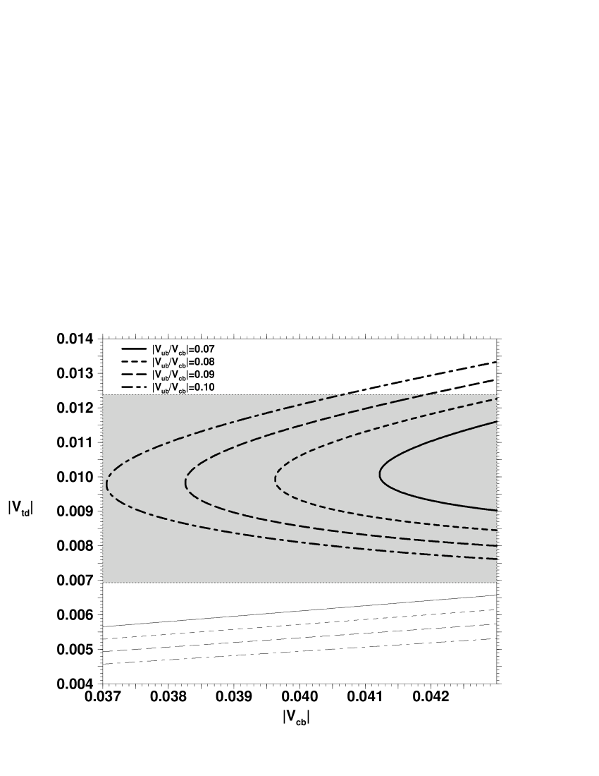
FIG. 3.: The dependence of $|V_{td}|$ on $V_{cb}$ for $B_{K}=0.75$, $m_{t}^{\star}=168\,\text{GeV}$ and four values of $|V_{ub}/V_{cb}|$. The thin lines correspond to $\delta=0$, i.e. no CP-violation. The shaded area is consistent with $x_{d}$ from (70).

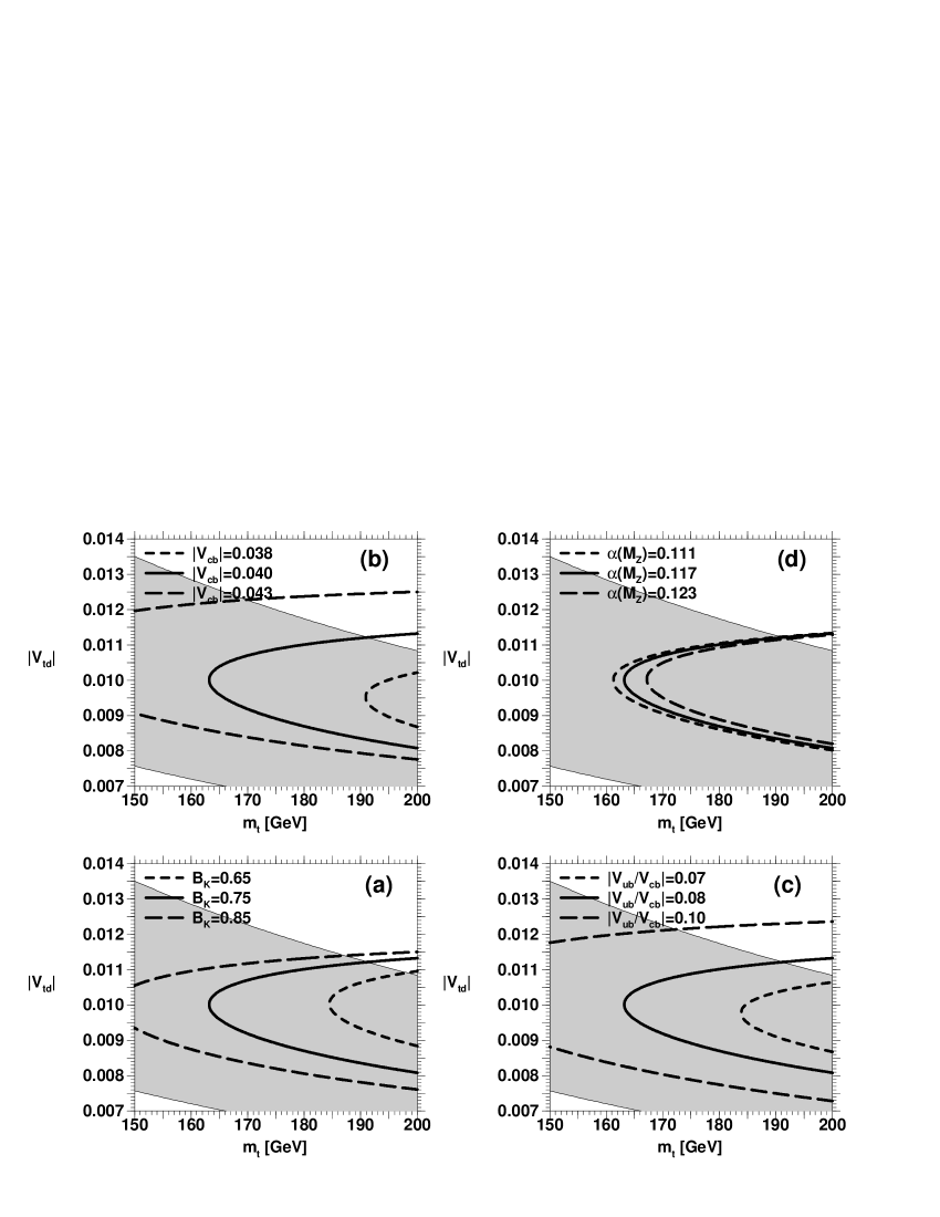
FIG. 4.: The dependence of $|V_{td}|$ on $m_{t}^{\star}$ for three values of (a) $B_{K}$, (b) $V_{cb}$, (c) $|V_{ub}/V_{cb}|$ and (d) $\alpha(M_{Z})$. All other parameters equal their central values of sect. III C. The shaded area gives the band (70) of $|V_{td}|$’s allowed by the ${\text{B}_{d}^{0}\!-\!\overline{\text{B}^{0}_{d}}}\,$-mixing parameter $x_{d}$. For large values of the discussed parameters $x_{d}$ favors the smaller branch of the solution.

FIG. 5.: The dependence of $\text{Im}\,\lambda_{t}$ on $m_{t}^{\star}$ for (a) three values of $|V_{cb}|$ and (b) four values of $|V_{ub}/V_{cb}|$. In plot (a) one observes that the higher solution for $\text{Im}\,\lambda_{t}$ is stable with respect to the variation of $|V_{cb}|$, whereas the lower branch depends quite strongly on this parameter.

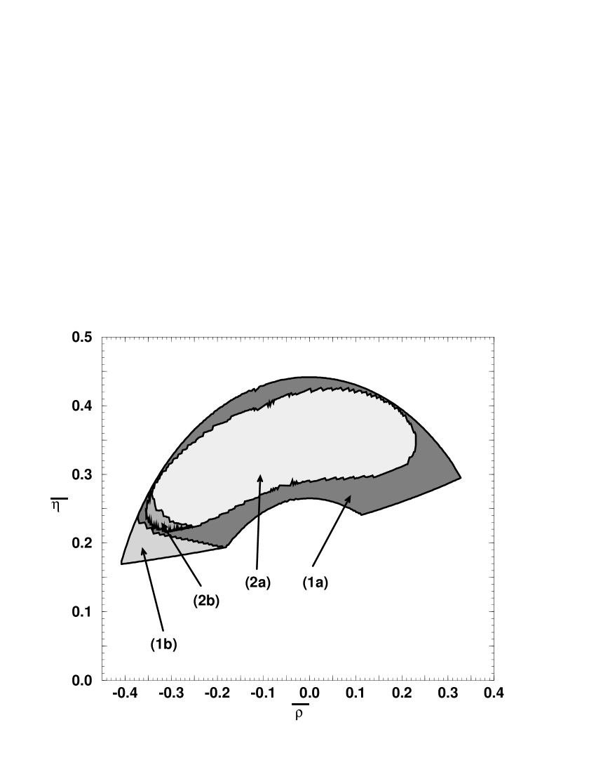
FIG. 6.: The allowed region for the pair $(\bar{\rho},\bar{\eta})$ consistent with $\varepsilon_{K}$ and $x_{d}$. Area (1a) is obtained from a scan over the full parameter range of sect. III C. Region (2a) corresponds to the parameters in the $1\sigma$ ellipsoid (76). Areas (1b) and (2b) are consistent with $\varepsilon_{K}$, but not with $x_{d}$.

VI A 1995 look at the ${\text{\bf K}_{\text{\bf L}}\!-\!\text{\bf K}_{\text{\bf S}}}\,$-mass difference

In this section we will have a look at the status of the ${\text{K}_{\text{L}}\!-\!\text{K}_{\text{S}}}\,$-mass difference $\Delta m_{K}$.

The short distance part of $\Delta m_{K}$, denoted by $(\Delta m_{K})_{\text{SD}}$, reads

$$\frac{\left(\Delta m_{K}\right)_{\text{SD}}}{m_{K}} = \frac{G_{F}^{2}}{6\pi^{2}}f_{K}^{2}B_{K}M_{W}^{2}$$ (106)

$$\cdot\left[\left(\text{Re}\,\lambda_{c}\right)^{2}x_{c}^{\star}\eta_{1}^{\star}+2\left(\text{Re}\,\lambda_{c}\right)\left(\text{Re}\,\lambda_{t}\right)S\left(x_{c}^{\star},x_{t}^{\star}\right)\eta_{3}^{\star}+\left(\text{Re}\,\lambda_{t}\right)^{2}S\left(x_{t}^{\star}\right)\eta_{2}^{\star}\right],$$

where the small imaginary parts of $\lambda_{c}$ and $\lambda_{t}$ have been neglected. The three terms in the brackets contribute roughly in the ratio 100:10:1, therefore the term containing $\eta_{1}^{\star}$ is most important, the one with $\eta_{2}^{\star}$ is least.

Because $\eta_{1}^{\star}$ strongly depends on its input parameters, especially on $m_{c}^{\star}$ and $\Lambda_{\overline{\text{MS}}}^{\text{NLO}}$, it does not make sense to use the constant defined in (15). We therefore calculate $\eta_{1}^{\star}$ for each set of parameters in our numerical evaluation. Inserting our standard set of values defined in sect. III C, we obtain

$$\frac{\left(\Delta m_{K}\right)_{\text{SD}}}{\left(\Delta m_{K}\right)_{\text{exp}}} = \left\{\begin{array}[]{rl@{\hspace{1cm}}rl}0.52&{+0.17\atop-0.11}\hfil\hskip 28.45274pt&\text{for}&\Lambda_{\overline{\text{MS}}}^{\text{NLO}}=0.210\,\text{GeV}\\ 0.67&{+0.25\atop-0.14}\hfil\hskip 28.45274pt&\text{for}&\Lambda_{\overline{\text{MS}}}^{\text{NLO}}=0.310\,\text{GeV}\\ 0.91&{+0.39\atop-0.20}\hfil\hskip 28.45274pt&\text{for}&\Lambda_{\overline{\text{MS}}}^{\text{NLO}}=0.410\,\text{GeV}\end{array}\right.$$ (110)

The errors are estimated by a scan through the allowed parameter space and includes the error stemming from scale variations in the $\eta_{i}^{\star}$’s.

The strong $\Lambda_{\overline{\text{MS}}}^{\text{NLO}}$ dependence of $\left(\Delta m_{K}\right)_{\text{SD}}/\left(\Delta m_{K}\right)_{\text{exp}}$ has been visualized in fig. 7. The central line is obtained by using the central values defined in sect. III C, the band shaded in grey displays the error.

For large values of $\Lambda_{\overline{\text{MS}}}^{\text{NLO}}$ the uncertainties in $\eta^{\star}_{1}$ due to scale variations become large indicating the breakdown of perturbation theory. Therefore the error bar on $\Delta m_{K}$ which is then dominated by this scale uncertainty grows very large prohibiting a precise prediction for the mass difference. One will have to see, whether in the future $\Lambda_{\overline{\text{MS}}}^{\text{NLO}}$ will continue growing in the future and thereby bringing the next-to-leading order result for $\eta^{\star}_{1}$ into troubles.

Let us now discuss the differences between our new result and previous analyses: In most textbooks $\Delta m_{K}$ is termed to be dominated by poorly calculable long-distance physics. Yet by power counting arguments, long-distance effects should be suppressed by a power of $\Lambda_{\text{QCD}}^{2}/m_{c}^{\star\,2}$ with respect to the short distance part because the coefficient of the leading dimension six operator contributing to the $\eta^{\star}_{1}$-part of the effective Hamiltonian in (3) is proportional to $m_{c}^{\star\,2}$ (see e.g. [33]).

A short look at (110) clearly exhibits a short distance dominance. Let us discuss the steps which have guided us to this result.

Already our 1993 analysis [6], in which we have calculated the coefficient $\eta^{\star}_{1}$ in the next-to-leading order approximation, has resulted in a large enhancement of the theoretical prediction for the ${\text{ K}^{0}\!-\!\overline{\text{K}^{0}}}\,$-mixing. This fact is true, because

• the next-to-leading order correction have largely increased the value of $\eta^{\star}_{1}$ and

• the experimental value for $\Lambda_{\overline{\text{MS}}}^{\text{NLO}}$ has risen in the last decade.

Both findings lead to the drastic increase of $\eta_{1}^{\star}$ by approximately 65%, which we get by comparing (16) and (15).

Finally, our new analysis compared to [6] for the first time uses the coefficient $\eta_{3}^{\star}$ calculated in the next-to-leading approximation. This quantity again enlarges the result for $\Delta m_{K}$. Because $\Lambda_{\overline{\text{MS}}}^{\text{NLO}}$ has grown again in the meantime thereby enlarging the theoretical prediction once more, we are now able to reproduce the experimentally measured value to 50–100% by short distance physics.

Some authors attributed the deficit in $\Delta m_{K}$ to new physics. The large scale uncertainties present in the coefficient $\eta_{1}^{\star}$, which obscure a clean determination of the Standard Model contribution, make the ${\text{ K}^{0}\!-\!\overline{\text{K}^{0}}}\,$-mixing a poor laboratory to search for the impact of new physics.

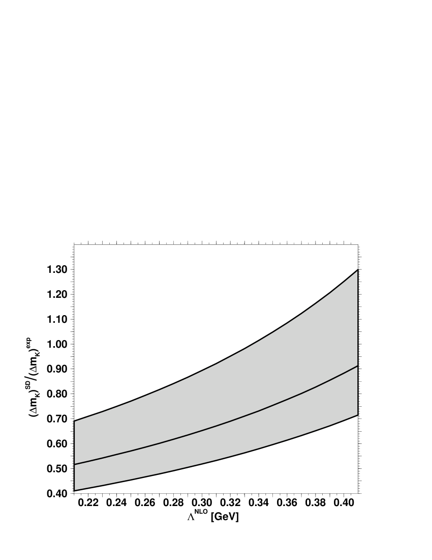
FIG. 7.: The dependence of the ratio of the short distance part of the ${\text{ K}^{0}\!-\!\overline{\text{K}^{0}}}\,$-mixing to the experimentally measured value on $\Lambda^{\text{NLO}}\equiv\Lambda_{\overline{\text{MS}}}^{\text{NLO}}$. The curve in the middle is obtained by choosing the central values of the parameters as given in sect. III C. All values lying in the shaded area are compatible within the error bands quoted in this section. The increasing height of the band displaying the error is due to the growing scale uncertainties present in the coefficient $\eta_{1}^{\star}$.

REFERENCES

-
[1]
J. H. Christenson, J. W. Cronin,
V. L. Fitch and R. Turlay,
Phys. Rev. Lett. 13 (1964) 138.
J. H. Christenson, J. W. Cronin, V. L. Fitch and R. Turlay, Phys. Rev. 140B (1965) 74. - [2] L. Chau, Phys. Rep. 95 (1983) 1. A. J. Buras and M. K. Harlander, A Top-Quark Story: Quark Mixing, CP-Violation and Rare Decays in the Standard Model, in Heavy Flavours, ed. A. J. Buras and M. Lindner, World Scientific, Singapore, 1993.
- [3] T. Inami and C. S. Lim, Progr. Theor. Phys. 65 (1981) 297 [Erratum: 65 (1981) 1772].
- [4] F. J. Gilman and M. B. Wise, Phys. Rev. D27 (1983) 1128.
-
[5]
J. M. Flynn, Mod. Phys. Lett. A5 (1990) 877.
A. Datta, J. Fröhlich and E. A. Paschos, Z. Phys. C46 (1990) 63. - [6] S. Herrlich and U. Nierste, Nucl. Phys. B419 (1994) 292.
- [7] A. J. Buras, M. Jamin and P. H. Weisz, Nucl. Phys. B347 (1990) 491.
- [8] S. Herrlich and U. Nierste, The complete –hamiltonian in next-to-leading order, preprint TUM-T31-86/95 in preparation.
- [9] Particle Data Group, Phys. Rev. D50 (1994) 1173.
- [10] A. J. Buras, M. E. Lautenbacher and G. Ostermaier, Phys. Rev. D50 (1994) 3433.
- [11] L. Wolfenstein, Phys. Rev. Lett. 51 (1983) 1945.
- [12] A. J. Buras, M. Jamin and P. H. Weisz, Nucl. Phys. B408 (1993) 209.
- [13] P. Ball, M. Beneke and V.M. Braun, preprint CERN-TH/95-65,hep-ph/9503492.
- [14] I. Bigi, Plenary talk at the DPG conference, Karlsruhe 1995.
- [15] P. Ball and U. Nierste, Phys. Rev. D50 (1994) 5841.
- [16] O. Podobrin, Plenary talk at the DPG conference, Karlsruhe 1995.
- [17] F. Abe et al., CDF, Phys. Rev. D50 (1994) 2966, Phys. Rev. Lett.73 (1994) 225.
- [18] S. Riemann, Plenary talk at the DPG conference, Karlsruhe 1995.
- [19] S. Abachi et al., D0, FERMILAB-PUB 1995.
- [20] D. E. Soper, Summary of the XXX Recontre de Moriond, QCD Session, hep-ph/9506218.
-
[21]
W. A. Bardeen, A. J. Buras and J.-M. Gérard,
Phys. Lett. B211 (1988) 343.
J.-M. Gérard, Acta Phys. Pol. B21 (1990) 257. - [22] J. F. Donoghue, E. Golowich and B. R. Holstein, Phys. Lett. B119 (1982) 412.
-
[23]
A. Pich and E. de Rafael, Phys. Lett. B158 (1985) 477.
J. Prades et al., Z. Phys. C51 (1991) 287. - [24] J. Bijnens and J. Prades, NORDITA-95/11, hep-ph/9502363.
- [25] M. Crisafulli et al., hep-lat/9505020.
- [26] N. Ishizuka et al., Phys. Rev. Lett. 71 (1993) 24.
- [27] S. Bethke, Proc. of the Summer School on Hadronic Aspects of Collider Physics, Zuoz, Switzerland, August 1994.
-
[28]
A. Duncan, E. Eichten, J. Flynn, B. Hill, G. Hockney and
H. Thacker, preprint FERMILAB-PUB-94/164-T,
hep-lat/9407025.
C.W. Bernard, J.N. Labrenz and A. Soni, Phys. Rev. D D49 (1994) 2536.
T. Draper and C. McNeile, Nucl. Phys. (Proc. Suppl.) 34 (1994) 453. -
[29]
E. Bagan, P. Ball, V.M. Braun and H.G. Dosch, Phys. Lett.
B278 (1992) 457.
M. Neubert, Phys. Rev. D45 (1992) 2451. - [30] A. J. Buras, Phys. Lett. B317 (1993) 449.
- [31] A. Ali and D. London, preprint DESY-93-022, to be publ. in Proc. of ECFA Workshop on the Physics of a B Meson Factory, ed. R. Aleksan, A. Ali (1993).
- [32] K. Jakobs, ALEPH, Talk at the DPG conference, Karlsruhe 1995.
- [33] M. A. Shifman, Int. J. of Mod. Phys. A12 (1988) 2769.