The resummed Drell-Yan cross section in the double-logarithmic approximation suffers from infrared renormalons. Their presence was interpreted as an indication for non-perturbative corrections of order $\Lambda_{\rm QCD}/(Q(1-z))$. We find that, once soft gluon emission is accurately taken into account, the leading renormalon divergence is cancelled by higher-order perturbative contributions in the exponent of the resummed cross section. From this evidence, ‘higher twist’ corrections to the hard cross section in Drell-Yan production should intervene only at order $\Lambda_{\rm QCD}^{2}/((Q^{2}(1-z)^{2})$ in the entire perturbative domain $Q(1-z)>\Lambda_{\rm QCD}$. We compare this result with hadronic event shape variables, comment on the potential universality of non-perturbative corrections to resummed cross sections, and on possible implications for phenomenology.

submitted to Nuclear Physics B

1 Introduction

The factorization theorems of QCD [1] allow a rigorous treatment of ‘hard processes’, since the non-perturbative dynamics can be isolated in a few universal distribution and fragmentation functions. The classical case for this approach is the Drell-Yan (DY) process $h_{a}+h_{b}\to\mu^{+}\mu^{-}+X$, when a muon pair (or, alternatively, a massive vector boson) with invariant mass $Q^{2}$ is produced in the collision of two hadrons, $h_{a}$, $h_{b}$, with invariant mass $s$. The cross section is then given by [1]

$$\frac{\mbox{d}\sigma}{\mbox{d}Q^{2}}=\sigma_{0}\,W(s,Q^{2})\qquad\sigma_{0}=\frac{4\pi\alpha_{\rm QED}^{2}}{9Q^{2}s}$$ (1.1)

$$W(s,Q^{2})=\sum_{i,j}\int\limits_{0}^{1}\frac{\mbox{d}x_{i}}{x_{i}}\,\frac{\mbox{d}x_{j}}{x_{j}}f_{i/h_{a}}(x_{i},Q^{2})f_{j/h_{b}}(x_{j},Q^{2})\,\omega_{ij}(z,\alpha_{s}(Q))\,+\,{\cal O}\!\left(\left(\frac{\Lambda_{\rm QCD}}{Q}\right)^{k}\right)\,,$$ (1.2)

where $f_{i/h_{a}}(x_{i},Q^{2})$ ($f_{j/h_{b}}(x_{j},Q^{2})$) is the distribution function for a parton $i$ in $h_{a}$ (parton $j$ in $h_{b}$) and $z=Q^{2}/(x_{i}x_{j}s)$ is the ratio of invariant masses of the produced muon pair and the colliding hard partons. The ‘hard cross section’ $\omega_{ij}(z,\alpha_{s}(Q))$ can be expanded as a power series in the strong coupling $\alpha_{s}(Q)$. The separation of the Drell-Yan cross section into distribution functions and a hard cross section is not unique. We will take the DIS scheme for the distribution functions, so that for quarks and antiquarks, which is the only case we will be interested in, the distribution functions are given by the corresponding deep inelastic scattering (DIS) cross section. In the following we neglect the sum over parton species and consider only $i=q$, $j=\bar{q}$.

The DY process is one of the simplest, where one can realize, experimentally, a short-distance dominated dynamics involving two large but possibly disparate scales: When $1-z\ll 1$, the phase space for gluon emission is restricted, so that the actual scale of the emission process is $Q(1-z)$ rather than $Q$. Although soft divergences cancel, large finite corrections in the form of ‘+-distributions’ $\alpha_{s}(Q)^{n}[(\ln^{2n-1}(1-z))/(1-z)]_{+}$ are left over and it is necessary to resum them to all orders. As long as $Q(1-z)>\Lambda_{\rm QCD}$, the relevant contributions from soft and collinear partons are still amenable to perturbative analysis. The resummation (to single-logarithmic accuracy) has been completed in [2, 3].

The theoretical discussion is simplified in terms of moments. Introducing the DY scaling variable $\tau=Q^{2}/s$, eq. (1.2) can be written as

$$W(N,Q^{2})\equiv\int\limits_{0}^{1}d\tau\,\tau^{N-1}\,W(\tau,Q^{2})=f_{q/h_{a}}(N,Q^{2})f_{\bar{q}/h_{b}}(N,Q^{2})\,\omega_{q\bar{q}}(N,\alpha_{s}(Q))\,,$$ (1.3)

where $\omega_{q\bar{q}}(N,\alpha_{s}(Q))$ ($f_{q/h_{a}}(N,Q^{2})$) denotes moments of the hard cross section (distribution function) with respect to $z$ ($x_{i}$). For large $N$, the moments probe small $1-z$ with the correspondence rule $[(\ln^{n}(1-z))/(1-z)]_{+}\longleftrightarrow\ln^{n+1}N$. The large higher order corrections $\alpha_{s}(Q)^{n}\ln^{k}N$ ($k\leq 2n$) can be resummed systematically by [2, 3]

$$\omega_{q\bar{q}}(N,\alpha_{s}(Q)) = H(\alpha_{s}(Q))\,\exp\Bigg{[}\int\limits_{0}^{1}dz\,\frac{z^{N-1}-1}{1-z}\Bigg{\{}2\int\limits_{Q^{2}(1-z)}^{Q^{2}(1-z)^{2}}\frac{dk_{t}^{2}}{k_{t}^{2}}\,A(\alpha_{s}(k_{t}))$$ (1.4)

$$\hskip 85.35826pt+\,B(\alpha_{s}(\sqrt{1-z}Q))\Bigg{\}}\Bigg{]}+{\cal O}\!\left(\frac{\ln N}{N}\right)\,,$$

provided the functions $A(\alpha_{s})$ and $B(\alpha_{s})$ (to be detailed later) are known to some appropriate order.

In this paper we address the question of possible non-perturbative contributions to the resummed cross section in eq. (1.4), suppressed by powers of the large momentum $Q$ (‘power corrections’). We are motivated by the observation that the integrals in this equation include the regions of very small momenta $k_{t}$, which render the resummation of $\ln N$ sensitive to the infrared (IR) behaviour of the strong coupling. The resummed expression depends on the prescription how to deal with the IR Landau pole in the (perturbative) strong coupling or, in other words, on the value of an IR cutoff. It has been found [4, 5] that IR effects to the resummed formulas should intervene already at the order $\Lambda_{\rm QCD}/(Q(1-z))$, which suggests that to this accuracy the factorized hard cross section has to be complemented by (exponentiated) non-perturbative corrections.

If confirmed, this statement is of a considerable theoretical and phenomenological interest. For phenomenology, it would imply that non-perturbative corrections decrease so slowly that they are numerically important for data analysis even at the largest available energies. For a theoretician, the problem is especially interesting because without guidance of the operator product expansion there is no immediate classification of power corrections and one must rely on different methods.

The approach applied in [4, 5] and in this paper utilizes the fact that the insufficiency of perturbation theory to account for the region of momenta of order $\Lambda_{\rm QCD}$ is indicated by the perturbative expansion itself, through the appearence of another type of large perturbative corrections in large orders. These corrections, proportional to $\alpha_{s}(Q)^{n}\,n!$ and known as infrared (IR) renormalons [6], cause the divergence of the perturbative expansion. The numerical value attached to such a divergent series depends on the summation prescription. Since, according to current understanding, QCD is the theory of strong interactions, this prescription dependence must be cancelled by all those contributions that elude a perturbative treatment. By this argument one can determine the order in $\Lambda_{\rm QCD}/Q$ at which non-perturbative corrections must enter, or, in other words, the level of theoretical accuracy beyond which perturbative QCD must fail. For processes that allow an operator product expansion like in DIS, the renormalon approach is complementary and less powerful than the operator product expansion. In the case of resummed cross sections the consideration of IR renormalons or, equivalently, IR cutoff dependence in perturbation theory can provide genuinely new information on the nature of non-perturbative corrections. The results of [4, 5] suggest that non-perturbative corrections are expected to affect the resummed DY cross section at the level of $1/Q$. Corrections of this size were also detected for hadronic event shape variables [7, 8]. Since the evolution equations that govern soft gluon emission are universal, it was proposed that non-perturbative corrections of order $1/Q$ can be described by a single parameter common to all resummed cross sections [8, 9, 10].

In this paper we reanalyze this problem. Our main result can be summarized by the statement that the structure of IR renormalons and power corrections depends crucially on soft gluon emission at large angles so that the collinear approximation does not apply. The phase space is then much more complicated and process-dependent. To obtain information on soft gluon emission to power-like accuracy, the functions $A$ and $B$ in eq. (1.4) need to be kept to all orders. In particular, the leading IR renormalon divergence (implying $1/Q$-corrections) of the resummed DY cross section found in [4, 5] appears as an artefact of using a finite-order approximation for these functions. The apparent $1/Q$-ambiguities in the ‘standard’ factorized formula eq. (1.4) are cancelled a zero in higher order perturbative corrections and the remaining power corrections appear to be of order $N^{2}\Lambda_{\rm QCD}^{2}/Q^{2}$. This cancellation is in effect similar (though the physics is different) to the cancellation of the leading $1/m_{Q}$ ambiguities between the phase-space and the series of radiative corrections to the decay widths of heavy particles [11, 12, 13]. Our results are obtained in a certain approximation to large-order behaviour. To go beyond this approximation, two-gluon emssion would have to be analyzed to power-like accuracy. The fact that even for one-gluon emission the correct IR renormalon structure follows only from all-order expressions for $A$ and $B$ makes this a vastly complicated problem.

Since the language connected with large-order behaviour appears rather formal it is helpful to recall the following correspondence which reveals more physical insight: For processes to which the operator product expansion can be applied, the power corrections deduced from renormalons can be identified with contributions of operators of higher dimension (twist). The above prescription dependence translates into the ambiguity in the choice of factorization scale below which fluctuations are called ‘soft’ and therefore should be included into the definition of the matrix elements of higher-twist operators. For perturbative contributions this factorization scale acts as an IR cutoff. Therefore, more generally, quite in analogy to the large perturbative corrections of type $\alpha_{s}(Q)^{n}[(\ln^{2n-1}(1-z))/(1-z)]_{+}$ discussed previously, the large factorials $\alpha_{s}(Q)^{n}\,n!$ can also be understood [12] as remnants from the Kinoshita-Lee-Nauenberg infrared cancellations, provided an IR regularization with an explicit mass scale such as a finite gluon mass $\lambda$ is used. Instead to factorials in large orders, one can then restrict attention to cutoff dependences like $\lambda/Q$, $\lambda^{2}/Q^{2}\ln\lambda^{2}$ in lowest order radiative corrections, which is physically more intuitive. For IR safe quantities, explicit IR divergences vanish by construction, while the scaling of power corrections can be determined by setting the IR cutoff to $\Lambda_{\rm QCD}$. In this language, we find that potential contributions to Drell-Yan production of order $\lambda/Q$ from the restriction on the phase space are exactly cancelled by the contributions of the same order to the matrix elements.

The paper is organized as follows: In Sect. 2 we analyze the exponent in eq. (1.4). We reproduce the results of [4, 5] in the approximation adopted in these works and proceed to show that low-order truncations of the functions $A$ and $B$ are insufficient to draw definite conclusions about non-perturbative corrections to the exponent. We outline three possible scenarios for the complete result. To distinguish the correct one, an all-order calculation beyond the soft and collinear approximation is required. We introduce and justify the corresponding (still approximate) all-order calculation in Sect. 2.3. Those readers who prefer to think in terms of IR cutoff dependence rather than large-order behaviour might ignore subsection 2.3.

In Sect. 3 we calculate the partonic DY and DIS cross sections with finite gluon mass $\lambda$ to first order in the strong coupling and extract the hard scattering function $\omega_{q\bar{q}}(z,\alpha_{s}(Q))$. We find that all potential corrections of order $N\lambda/Q$ cancel, so that the one-loop perturbative result is protected from IR contributions to this accuracy. As mentioned previously this calculation has a dual interpretation in terms of either cutoff dependence or large-order behaviour. At this stage we can conclude that at present there is no evidence for nonperturbative corrections of order $N\Lambda_{\rm QCD}/Q$ to the DY cross section. To trace the origin of this cancellation, we repeat the calculation in the soft limit in Sect. 4, but with a cutoff on the energy and transverse momentum of emitted gluons. This allows us to pin down the phase space approximation, in which the DLA looses terms of order $N\Lambda_{\rm QCD}/Q$ and clarifies the relevance of soft emission at large angles.

In Sect. 5 we follow the approach of [14] to derive the soft factorization for the DY cross section in terms of Wilson lines. We calculate the corresponding Wilson line with an arbitrary number of fermion loop insertions in the gluon line and check that the result satisfies the correct renormalization group equation (evolution equation). We find that all relevant anomalous dimensions (in the $\overline{\rm MS}$ scheme) are entire functions in the Borel plane and the IR renormalons enter only through the initial (boundary) condition for the evolution. The apparent $1/Q$-corrections to the standard result eq. (1.4) are due to an unfortunate choice of particular solution of the evolution equation for the Wilson line which in turn necessitates a more singular homogeneous solution than actually required. As a result, the apparent IR renormalon that indicates $1/Q$-corrections in the Borel transform of the exponent in eq. (1.4) is cancelled by a ‘hidden’ zero in the sum of Borel transforms of the (redefined) anomalous dimensions, which becomes manifest only if these are calculated to all orders. We discuss a possibility to reformulate the standard factorization formulas for DY cross sections in such a way that the cancellation of leading renormalons is explicit.

In Sect. 6 we summarize, compare our results with those for thrust averages in $e^{+}e^{-}$ annihilation and comment on potential implications for processes other than Drell-Yan. Appendix A contains a rederivation of the cusp anomalous dimension of the Wilson line, and in Appendix B we compare typical phase-space integrals for the DY cross section and the thrust distribution.

2 Anatomy of the exponent

In this section we discuss the exponent in the resummed hard cross section. We rewrite eq. (1.4) as

$$\omega_{q\bar{q}}(N,\alpha_{s}(Q))=H(\alpha_{s}(Q))\,\exp\left[E(N,\alpha_{s}(Q))\right]+R(N,\alpha_{s}(Q))\,,$$ (2.1)

where $R(N,\alpha_{s}(Q))$ vanishes as $N\to\infty$ and the exponent is given by

$$E(N,\alpha_{s}(Q))=\int\limits_{0}^{1}dz\,\frac{z^{N-1}-1}{1-z}\Bigg{\{}2\!\!\int\limits_{Q^{2}(1-z)}^{Q^{2}(1-z)^{2}}\!\frac{dk_{t}^{2}}{k_{t}^{2}}\,A(\alpha_{s}(k_{t}))+B(\alpha_{s}(\sqrt{1-z}Q))+C(\alpha_{s}((1-z)Q))\Bigg{\}}\,.$$ (2.2)

The exponent expanded in $\alpha_{s}(Q)$ contains terms $\alpha_{s}(Q)^{n}\ln^{k}N$ with $k\leq n+1$. To sum all logarithms with $k\geq n+1-m$, the expansion coefficients of $A(\alpha_{s})\equiv\sum_{m=0}a_{n}\alpha_{s}^{m+1}$ up to order $m+1$ and of $B$ and $C$ up to order $m$ are required, as well as the $\beta$-function that controls evolution of the coupling to order $\alpha_{s}^{m+1}$. $A$ is a process-independent function, which can be identified with the eikonal (or cusp) anomalous dimension. Up to second order it is given by [15]

$$a_{0}=\frac{C_{F}}{\pi}\qquad a_{1}=\frac{C_{F}}{2\pi^{2}}\left[C_{A}\left(\frac{67}{18}-\frac{\pi^{2}}{6}\right)-\frac{5}{9}N_{f}\right]\,.$$ (2.3)

$B$ and $C$ are process-specific. $B$ involves the underlying DIS process, while $C$ comes only from the DY process. Their first order expressions are

$$b_{0}=-\frac{3}{2}\frac{C_{F}}{\pi}\,,\qquad c_{0}=0\,.$$ (2.4)

Note that compared to the conventional form [3] quoted in eq. (1.4) we have reintroduced a third function $C$ with expansion in the coupling normalized at $(1-z)Q$ as it was originally present in the analysis of [2]. With the coefficients given above, $C$ is irrelevant for summing logarithms to next-to-leading accuracy ($k\geq n$) and can be dropped for this purpose [16, 17]. The reason for keeping this function in the present context will become clear in Sect. 5. The function $C$ can be dispensed of by a redefinition of $A$ and $B$ [17]. However, the interpretation of $A$ as universal cusp anomalous dimension is then lost beyond order $\alpha_{s}^{2}$.

We are now interested in the infrared sensitivity of the exponent. Perturbatively, it is most directly visible through the presence of the Landau pole of the perturbative running coupling inside the integration regions in eq. (2.2). The Landau pole has two (related) consequences. It leads to IR renormalons in the re-expansion of $E$ in $\alpha_{s}(Q)$ and renders the integrals dependent on the treatment of the pole. The ambiguities that arise in this way quantify our ignorance on the correct infrared behaviour, which does not show a Landau pole. Since extracting the ambiguities from the Landau pole essentially projects on the infrared regions of integrals, the same conclusions can be obtained from eliminating these regions by an explicit IR cutoff and by studying the dependence on the cutoff. In Sect. 2.1 we reproduce the result on power corrections in [4] obtained in the double-logarithmic approximation. The general case is developed in Sect. 2.2. We introduce and justify an approximation to calculate large-order behaviour in Sect 2.3.

2.1 Ambiguities to double-logarithmic accuracy

The double-logarithmic approximation (DLA) corresponds to exponentiation of the $\alpha_{s}(Q)\ln^{2}N$-term in $\omega_{q\bar{q}}(N,\alpha_{s}(Q))$. In eq. (2.2), only $a_{0}$ has to be kept. We remove the contribution from gluons with energy less than $\mu>\Lambda_{\rm QCD}$. Since $Q(1-z)/2$ can be interpreted as the energy of the emitted gluon (for small $1-z$), we obtain

$$E^{\rm DLA}(N,\alpha_{s}(Q),\mu) = \int\limits_{0}^{1-2\mu/Q}dz\,\frac{z^{N-1}-1}{1-z}\,\,2a_{0}\!\!\int\limits_{Q^{2}(1-z)}^{Q^{2}(1-z)^{2}}\!\frac{dk_{t}^{2}}{k_{t}^{2}}$$ (2.5)

$$= {\mbox{$\mu$-independent}}+2a_{0}\alpha_{s}(Q)\,(N-1)\frac{\mu}{Q}\ln\frac{\mu^{2}}{Q^{2}}+{\cal O}\!\left(\frac{\mu}{Q}\right)\,.$$

Notice the linear dependence on the cutoff and the large coefficient proportional to $N$. In [4] the ambiguity of the exponent due to the Landau pole has been evaluated in the approximation of one-loop running for the coupling,

$$\alpha_{s}(k)=\frac{\alpha_{s}(Q)}{1-\beta_{0}\alpha_{s}(Q)\ln(k^{2}/Q^{2})}=\frac{1}{(-\beta_{0})\ln(k^{2}/\Lambda_{\rm QCD}^{2})}\,,$$ (2.6)

where $\beta_{0}=-1/(4\pi)(11-2N_{f}/3)$ is the lowest-order coefficient of the $\beta$-function. Following the approximation of [4] we keep only the term $a_{0}\alpha_{s}(k_{t})$ up to terms that give ambiguities of order $1/Q^{2}$. The $k_{t}$-integral produces a cut starting at $z=1-\Lambda_{\rm QCD}/Q$. Evaluating the $z$-integral above or below the cut, we find the difference (neglecting terms of order $(\Lambda_{\rm QCD}/Q)^{2}$)

$$\delta E^{\rm DLA}(N,\alpha_{s}(Q)) = \frac{1}{2\pi i}\int\limits_{0}^{1}dz\frac{z^{N-1}-1}{1-z}\,2a_{0}\left(-\frac{1}{\beta_{0}}\right)\,\mbox{disc}\left[\ln\ln(1-z)^{2}\frac{Q^{2}}{\Lambda_{\rm QCD}^{2}}\right]$$ (2.7)

$$= 2a_{0}(N-1)\left(-\frac{1}{\beta_{0}}\right)\frac{\Lambda_{\rm QCD}}{Q}+{\cal O}\!\left(\left(\frac{N\Lambda_{\rm QCD}}{Q}\right)^{2}\right)\,.$$

The cutoff dependence of eq. (2.5) and the ambiguity in eq. (2.7) agree, if we choose $\mu\sim\Lambda_{\rm QCD}$, since $\alpha_{s}(Q)\ln(\Lambda_{\rm QCD}^{2}/Q^{2})=(-1/\beta_{0})$. It can be shown [18] that the ambiguity does not change qualitatively, if the coefficients $a_{1}$ and $b_{0}$ are included as required for the summation of next-to-leading logarithms $\alpha_{s}(Q)^{n}\ln^{n}N$. We therefore conclude that with the truncated series for $A$ and $B$ sufficient to sum next-to-leading logarithms, the exponent in the form of eq. (2.2) is prescription-dependent by terms of order $N\Lambda_{\rm QCD}/Q$, if the expression for the running coupling is not expanded and truncated. At this point, however, it is not clear whether these terms are artefacts of the approximations made or whether they should be interpreted as an indicator for ‘higher twist’ effects of this order as suggested in [4, 5]. To illustrate this point, we note that to the accuracy of summing next-to-leading logarithms one may replace [3]

$$z^{N-1}-1\to-\Theta\left(1-\frac{e^{-\gamma_{E}}}{N}-z\right)$$ (2.8)

It is easy to check that after this substitution the corresponding exponent $E$ has no ambiguities at all, unless $N>Q/\Lambda_{\rm QCD}$. Such large moments are excluded from consideration, since there is no perturbative treatment for them.

2.2 General case

In higher orders (contributing only to sub-dominant logarithms $\alpha_{s}(Q)^{n}\ln^{k}N$, $k<n$), the replacement in eq. (2.8) requires a redefinition of the functions $B$ and $C$. This suggests that for the purpose of identifying power corrections to the exponent, higher order coefficients of $A$, $B$ and $C$ are relevant, while they are not for a systematic summation of logarithms up to a certain accuracy. The discussion of ambiguities including higher order coefficients is simplified in terms of Borel transforms. We write the exponent as

$$E(N,\alpha_{s}(Q))=\left(-\frac{1}{\beta_{0}}\right)\int\limits_{0}^{\infty}du\,e^{-u/(-\beta_{0}\alpha_{s}(Q))}\,B[E](N,u)\,,$$ (2.9)

where for any function

$$f(\alpha_{s}(Q))=\sum_{n=0}^{\infty}f_{n}\alpha_{s}(Q)^{n+1}\quad\Longrightarrow\quad B[f](u)=\sum_{n=0}^{\infty}f_{n}(-\beta_{0})^{-n}\frac{u^{n}}{n!}\,.$$ (2.10)

Note the expansion parameter is $\alpha_{s}(Q)$. If $f$ has a term of order $\alpha_{s}(Q)^{0}$, it is treated separately. The ambiguities of $E$ due to the pole in the running coupling are now generated by IR renormalon poles of $B[E]$ in the $u$-integral. (These poles correspond to factorial divergence of the corresponding series expansion in $\alpha_{s}(Q)$.) A pole at $u=m$ leads to an ambiguity of order $(\Lambda_{\rm QCD}/Q)^{2m}$. The Borel representation allows us to write $B[E]$ in a factorized form. Let us continue to assume that $\beta(\alpha_{s})=\beta_{0}\alpha_{s}^{2}$, so that eq. (2.6) is exact. Then

$$B[\alpha_{s}(xQ)](x,u)=\sum_{n=0}^{\infty}\frac{(-1)^{n}}{n!}\ln x^{2}\,u^{n}=x^{-2u}\qquad B[\alpha_{s}(xQ)^{n}](x,u)=\frac{u^{n-1}}{n!}x^{-2u}\,,$$ (2.11)

so, for any function $f(\alpha_{s}(xQ))$,

$$B[f(\alpha_{s}(xQ))](x,u)=x^{-2u}\,B[f(\alpha_{s}(Q)](u)\,.$$ (2.12)

The $k_{t}$- and $z$-integrals that appear in $E$ can then be done and we obtain

$$B[E](N,u)=2\Delta_{1}(N,u)B[A](u)+\Delta_{2}(N,u)B[B](u)+\Delta_{3}(N,u)B[C](u)\,,$$ (2.13)

where all dependence on $N$ is factored into the functions

$$\Delta_{1}(N,u)=\frac{1}{u}\left(\frac{1}{2u}+\Gamma(N)\left[\frac{\Gamma(-u)}{\Gamma(N-u)}-\frac{\Gamma(-2u)}{\Gamma(N-2u)}\right]\right)\,,$$ (2.14)

$$\Delta_{2}(N,u)=\frac{1}{u}+\frac{\Gamma(N)\Gamma(-u)}{\Gamma(N-u)}\,,\qquad\Delta_{3}(N,u)=\Delta_{2}(N,2u)\,,$$ (2.15)

which depend only on the form of the exponent, but not on the details of the functions $A$, $B$, $C$. Note that $\Delta_{3}=\Delta_{2}-u\Delta_{1}$, so that

$$B[E](N,u)=\Delta_{1}(N,u)\left\{2B[A](u)-uB[C](u)\right\}+\Delta_{2}(N,u)\left[B[B](u)+B[C](u)\right]\,.$$ (2.16)

This is the observation that $C$ is in fact redundant [17] and can be absorbed into a redefinition of $A$ and $B$. If, as in Sect. 2.1, we keep only the coefficient $a_{0}$ of $A$, we obtain close to $u=1/2$,

$$B[E^{\rm DLA}](N,u)\stackrel{{\scriptstyle u\rightarrow 1/2}}{{=}}2a_{0}(N-1)\frac{2}{1-2u}\,.$$ (2.17)

The ambiguity of $E$ derived from eq. (2.9) (evaluating the integral above and below the pole) coincides with eq. (2.7). Without truncation of $A$ and $C$, we obtain

$$B[E](N,u)\stackrel{{\scriptstyle u\rightarrow 1/2}}{{=}}2(N-1)\frac{1}{1-2u}\left[2B[A]\left(\frac{1}{2}\right)-\frac{1}{2}B[C]\left(\frac{1}{2}\right)\right]\,,$$ (2.18)

assuming only that $B[A]$ and $B[C]$ are non-singular at $u=1/2$. Notice that the term $\Delta_{2}B[B]$ and the first term in square brackets of $\Delta_{1}$ which originate from the DIS subprocess do not lead to a singularity at $u=1/2$. The leading pole is at $u=1$, indicating power corrections of order $N\Lambda_{\rm QCD}^{2}/Q^{2}$, in agreement with the operator product expansion for deep-inelastic scattering, which constrains corrections to the leading-twist approximation to enter at order $1/Q^{2}$.

Hence, a conclusion regarding the presence of a pole at $u=1/2$ can not be obtained from finite-order approximations of $A$ etc., since the residue involves the Borel transforms at the point $u=1/2$. In other words: The presence of nonperturbative corrections of order $N\Lambda_{\rm QCD}/Q$ can only be discerned, if the anomalous dimension functions in the exponent are themselves defined to power-accuracy. Since the whole point of the resummation formula eq. (1.4) is to obtain certain large contributions to $\omega_{q\bar{q}}(N,\alpha_{s}(Q))$ to all orders by finite order calculations of $A$ etc., there is no compelling motivation to restrict attention to $E$ alone instead of the complete $\omega_{q\bar{q}}(N,\alpha_{s}(Q))$ for the purpose of identifying power corrections, because finite order approximations to the exponent are insufficient. But since the exponent captures all leading singular contributions $\ln^{k}N$ (but not singular terms $1/N\ln^{k}N$), one would still expect the exponent to indicate also the leading power corrections $(N\Lambda_{\rm QCD}/Q)^{k}$ (but not $1/N(N\Lambda_{\rm QCD}/Q)^{k}$). Regarding the presence of $N\Lambda_{\rm QCD}/Q$-corrections, the following three scenarios can be envisaged:

1. A renormalon ambiguity of order $N\Lambda_{\rm QCD}/Q$, i.e. a pole at $u=1/2$ is present. This situation is realized if $2B[A](u)-uB[C](u)$ is non-zero at $u=1/2$ and provided no cancellations with the remainder $R(N,\alpha_{s}(Q))$ occur, see C below. Then a nonperturbative correction of order $N\Lambda_{\rm QCD}/Q$ is required, and it has to exponentiate. This scenario is suggested by [4, 5].

2. The pole at $u=1/2$ cancels because

   $$2B[A]\left(\frac{1}{2}\right)-\frac{1}{2}\,B[C]\left(\frac{1}{2}\right)=0\,,$$ (2.19)

   and no ambiguity of order $N\Lambda_{\rm QCD}/Q$ remains. Then no nonperturbative corrections are required to this accuracy. Note that the Borel transforms of $A$, $B$ and $C$ could themselves have poles. Even in this case $B$ can not participate in the cancellation (if it occurs) at $u=1/2$, because $\Delta_{2}(N,1/2)\sim N^{1/2}$, while the residue of the pole at $u=1/2$ is of order $N$. Note also that after elimination of the redundant $C$ to arrive at the conventional eq. (1.4), the previous equation implies that the Borel transform of $A$ as it appears in eq. (1.4) has a zero at $u=1/2$. We will verify (in a certain approximation) that this zero is indeed present.

3. A further possibility is that the exponent does not incorporate all leading (in $N$ and $1/Q$) power corrections and the pole is cancelled with the remainder $R(N,\alpha_{s}(Q))$ in eq. (2.1). This can happen if the series for the remainder looks like (for large $n$)

   $$R(N,\alpha_{s}(Q))=\sum_{n}\alpha_{s}(Q)^{n+1}(-2\beta_{0})^{n}n!\,\frac{1}{N}\sum_{k=0}^{n}\frac{1}{k!}\ln^{k}N^{2}\,.$$ (2.20)

   To any finite order in $\alpha_{s}(Q)$ the remainder vanishes as $N\to\infty$, but its Borel transform

   $$B[R](N,u)=\frac{N^{4u-1}}{1-2u}$$ (2.21)

   has a pole at $u=1/2$ with residue proportional to $N$. A cancellation of this type would again imply that no nonperturbative corrections of order $1/Q$ are required, but that the soft factorization techniques break down to power-like accuracy.

To single out the correct scenario and clarify the size of expected nonperturbative corrections, $\omega_{q\bar{q}}(N,\alpha_{s}(Q))$ or at least the functions $A$, $C$ would have to be calculated to all orders. Obviously, this requires a certain approximation. In the following sections, we calculate a subset of higher order corrections and argue that this subset provides some generic insight. Before introducing this subset in the next subsection, we comment on the approximation of neglecting higher orders in the $\beta$-function in the derivation of eq. (2.13). When the next coefficient, $\beta_{1}$, is retained a simple factorized form as in eq. (2.13) is not immediate. However, provided the $\beta$-function itself does not have renormalons (as believed in the $\overline{\rm MS}$-scheme), inclusion of higher orders are expected only to turn the poles in $u$ into branch point singularities. The essence of the arguments above remains unaffected.

2.3 Higher order approximation

1

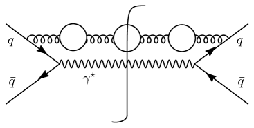
Figure 1: $\alpha_{s}^{4}$-contribution to the partonic Drell-Yan cross section. $\gamma^{\star}$ represents a photon with invariant mass $Q^{2}$ that splits into a lepton pair.

In calculating higher-order contributions to the DY hard cross section, we resort to an approximation that – despite its largely heuristic character – has proven useful in identifying IR renormalons and power corrections semi-quantitatively in other applications [20, 21]. The approximation consists in selecting the subset of higher-loop diagrams generated by insertion of an arbitrary number of fermion loops in the gluon line in diagrams contributing to the lowest order radiative correction, see Fig. 1 for an example. The corresponding series in $\alpha_{s}(Q)$ grows indeed as $\alpha_{s}(Q)^{n+1}n!$ and its Borel transform has the expected IR renormalon poles. The approximation (‘single-chain approximation’) has two immediate deficiencies which we discuss first. One may keep in mind that eventually the best justification for the single-chain approximation derives from its relation to IR cutoff dependence, which is discussed towards the end of this subsection.

The first observation is that each fermion loop is proportional to the abelian part of $\beta_{0}$, i.e. $N_{f}/(6\pi)$. The large-order behaviour from infrared regions is sign-alternating and does not lead to any ambiguities. Evidently, this happens because with fermion loops alone, there is no IR Landau pole in the running coupling. The usual way to deal with this deficiency is to restore the non-abelian $\beta_{0}$ by hand. This is justified by the expectation that the factorial behaviour is related to evolution of the coupling so that all other uncalculated diagrams would combine to reproduce this ad-hoc manipulation, up to an overall normalization, which is of minor interest for the parametric size of power corrections. The single-chain approximation then amounts to integrating the lowest order corrections with the complete (but still approximate) gluon propagator $\alpha_{s}(k)/k^{2}$. This deficiency is not specific to the DY process, but common to all previous applications [20, 21].

A more specific draw-back of the single-chain approximation is that within the selected set of diagrams, exponentiation of soft and collinear logarithms $\ln N$ does not occur. The calculated diagrams are those with the largest number of factors $N_{f}$ (the number of massless fermions) and give at most $\alpha_{s}(Q)^{n}\ln^{n+1}N$ (This remains obviously true after restoring the non-abelian $\beta_{0}$.). The dominant terms in the large-$N$ limit, $\alpha_{s}(Q)^{n}\ln^{k}N$ ($n+1<k\leq 2n$, $n>1$), come from diagrams with two or more gluon lines (chains). They can be partially obtained by exponentiation of the single-chain result, but in any case exponentiation leads outside the set of diagrams calculated exactly. Thus, if $\omega^{\rm(SC)}_{q\bar{q}}(N,\alpha_{s}(Q))$ denotes radiative corrections in the single-chain approximation (SCA), normalized to the tree-level hard cross section,

$$\ln\left[1+\omega^{\rm(SC)}_{q\bar{q}}(N,\alpha_{s}(Q))\right]=\omega^{\rm(SC)}_{q\bar{q}}(N,\alpha_{s}(Q))+\mbox{terms beyond SCA}\,.$$ (2.22)

These terms are of order $((\ln N)/N_{f}))^{k}$ relative to $\omega^{\rm(SC)}_{q\bar{q}}(N,\alpha_{s}(Q))$ so that the large-$N$ limit (the one we are interested in) does not commute with the large-$N_{f}$ limit (the one we calculate).

At this point, we note that the summation of soft and collinear $\ln N$’s has two aspects: The first is exponentiation as a consequence of an evolution equation, the second the arguments of the couplings that appear in the exponent, eq. (2.2). In the present investigation of power corrections to the DY process, as well as all previous ones [4, 5], we are mainly interested in the exponent and therefore the second aspect, which is independent of whether the evolution equation is an equation for $\ln\left[\omega_{q\bar{q}}(N,\alpha_{s}(Q))\right]$ or for $\omega_{q\bar{q}}(N,\alpha_{s}(Q))$ (in which case exponentiation does not occur). Indeed, the single-chain approximation gives a non-trivial series of higher-order corrections to the anomalous dimension functions $A$, $B$ and $C$ from subdominant logarithms in diagrams with fermion loops. The fact that this series exponentiates beyond the adopted approximation is secondary as long as one is interested only in the consequences of integration over the running coupling in the exponent. One could also say that it is more appropriate to think of this approximation as an approximation to $\ln\left[\omega_{q\bar{q}}(N,\alpha_{s}(Q))\right]$. When interpreted in this way, corrections are formally of order $1/N_{f}$ with no factor of $\ln N$ and the above non-commutativity of the large-$N$ and large-$N_{f}$ limit is, at least superficially, absent.

In the context of consequences of integration over the running coupling, it is more important that the single chain approximation is consistent with the fact that the appropriate scale in the coupling to sum large logarithms close to threshold is given by the transverse momentum of the emitted parton (gluon) [22]. The real emission correction to the partonic DY process in this approximation is schematically given by

$$W^{\rm real}(z,Q^{2})\sim\mbox{disc}_{k^{2}}\int\limits_{0}^{\infty}\frac{dk^{2}}{k^{2}}\int\frac{d|\vec{k}|d^{2}k_{t}}{(2\pi)^{3}2\sqrt{\vec{k}^{2}+k^{2}}}\,F(z;|\vec{k}|,k_{t};k^{2})\,\alpha_{s}(k)\,,$$ (2.23)

Kinematics dictates that the discontinuity is integrated up to $(k^{2})_{\rm max}\sim Q^{2}(1-z)^{2}$. Interchanging the order of the $k^{2}$- and $k_{t}$-integral, $k^{2}$ is integrated up to $k_{t}^{2}<Q^{2}(1-z)^{2}/4$ (for $z$ close to 1). Following the argument of [22] the $k^{2}$-integral can be evaluated up to subleading logarithms in $1-z$ by setting $k^{2}$ to the value at the upper limit of integration in all terms singular as $k^{2}\to 0$ and to zero elsewhere. Therefore

$$W^{\rm real}(z,Q^{2})\sim\int\frac{d^{3}\vec{k}}{(2\pi)^{3}2|\vec{k}|}\,F(z;|\vec{k}|,k_{t};0)\,\alpha_{s}(k_{t})\,,$$ (2.24)

up to subleading $\ln(1-z)$’s. The previous line gives simply the one-loop correction, but with $\alpha_{s}$ normalized at $k_{t}\sim Q(1-z)$. We see that the single-chain approximation is fully consistent with [22]: The only approximation is that the the gluon-propagator that enters the Schwinger-Dyson equation of [22] is given by $\alpha_{s}(k)/k^{2}$ in the single-chain approximation. In this approximation, the argument of the coupling is determined by the subprocesses in which the gluon line splits into the $\bar{q}q$ pair, with $k_{t}^{2}$ being the largest possible invariant mass of this pair, which is allowed by the kinematics of soft emission.

Let us emphasize that due to the approximations made to arrive at eq. (2.24), it can not be used immediately to deduce power-corrections. Also, there is no justification for integrating eq. (2.23) with $\alpha_{s}(k_{t})$ instead of $\alpha_{s}(k)$, since there is not even a formal limit in which such a replacement has a diagrammatic interpretation or would model a complete gluon propagator.

It is useful to observe that the Borel transform of radiative corrections in the single-chain approximation can be calculated as [12, 19, 23]

$$B\left[\omega^{\rm(SC)}_{q\bar{q}}\right](N,u)=-\frac{\sin(\pi u)}{\pi u}\,e^{5u/3}\int\limits_{0}^{\infty}d\lambda^{2}\left(\frac{\lambda^{2}}{Q^{2}}\right)^{-u}\frac{d}{d\lambda^{2}}\,\omega^{\rm(1)}_{q\bar{q}}(N,\lambda^{2}/Q^{2})\,,$$ (2.25)

where $\omega^{\rm(1)}_{q\bar{q}}(N,\lambda^{2}/Q^{2})\alpha_{s}(Q)$ denotes the one-loop correction to the hard cross section, calculated with a gluon of mass $\lambda$. The factor $5/3$ in the exponent arises, because we renormalize fermion loops in the $\overline{\rm MS}$ scheme.

Eq. (2.25) gives a transparent interpretation of IR renormalons in terms of IR cutoff dependence. By general properties of Mellin transforms, poles at positive $u$ on the left hand side of (2.25) are related to non-analytic terms (in $\lambda^{2}$) in the expansion of $\omega^{\rm(1)}_{q\bar{q}}(N,\lambda^{2}/Q^{2})$ for small $\lambda^{2}$. The existence of the pole in question, at $u=1/2$, is related to the presence of $\sqrt{\lambda^{2}}$, at $u=1$ to $\lambda^{2}\ln\lambda^{2}$ etc.. Indeed, instead of examining the large-order behaviour of perturbation theory to find hints for power corrections, it appears more direct to explore the IR cutoff dependence in lowest order. Then, just as an IR divergence $\ln\lambda^{2}$ in the partonic DY cross section indicates that the process is not IR safe but requires the introduction of IR sensitive distribution functions, the presence of further non-analytic terms indicates ‘higher twist’ nonperturbative corrections, at least with the adopted choice of leading-twist distribution functions.

Eq. (2.25) is technically convenient, because to calculate the hard cross section an IR regulator for intermediate steps is needed even in any case. Taking finite gluon mass instead of the more conventional dimensional regularization, the calculation differs from the one-loop calculation only in that we do not neglect terms that vanish as $\lambda\to 0$.

3 Hard cross section with IR cutoff

In this section we calculate the hard Drell-Yan cross section with finite IR regulator and investigate its cutoff dependence. The choice of gluon mass $\lambda$ as regulator is convienent because by eq. (2.25) the cutoff dependence can be translated into a statement on IR renormalons.

The calculation is a textbook problem. Since $\omega_{q\bar{q}}(z,\alpha_{s}(Q))$ does not depend on the particular initial state, one chooses to calculate the DY cross section and structure functions for quark states. It is convenient to introduce the dimensionless variable $\xi=\lambda^{2}/Q^{2}$. For the partonic DY and quark distribution function, let us write

$$W(\tau,Q^{2},\xi) = Q_{q}^{2}\left[\delta(1-\tau)+W^{\rm(1)}(\tau,\xi)+{\cal O}\left(\alpha_{s}(Q)^{2}\right)\right]$$

$$f_{q/q}(x,Q^{2},\xi) = \delta(1-x)+f_{q/q}^{\rm(1)}(x,\xi)+{\cal O}\left(\alpha_{s}(Q)^{2}\right)\,,$$ (3.1)

where $Q_{q}$ is the electric quark charge in units of electron charge. In the DIS scheme the distribution function is defined as

$$f_{q/q}(x,Q^{2})=\frac{F_{2}}{x}=-W^{\mu}_{\mu}+12x^{2}\frac{p_{\mu}p_{\nu}}{Q^{2}}W^{\mu\nu}\,.$$ (3.2)

$W^{\mu\nu}$ denotes the hadronic tensor for deep inelastic scattering from quarks with momentum $p$. According to eq. (1.2), the hard cross section is given by

$$\omega_{q\bar{q}}(z,\alpha_{s}(Q),\xi) = Q_{q}^{2}\left[\delta(1-z)+\omega_{q\bar{q}}^{\rm(1)}(z,\xi)+{\cal O}\left(\alpha_{s}(Q)^{2}\right)\right]$$

$$\omega_{q\bar{q}}^{\rm(1)}(z,\xi) = W^{\rm(1)}(z,\xi)-2f_{q/q}^{\rm(1)}(z,\xi)\,,$$ (3.3)

using equality of $f_{q/q}$ and $f_{\bar{q}/\bar{q}}$.

3.1 Partonic Drell-Yan cross section

The matrix element for

$$q(p_{1})+q(p_{2})\longrightarrow g(k)+\gamma^{\star}(q)$$ (3.4)

averaged (summed) over initial (final) colours and polarizations is given by

$$|{\cal M}|^{2}_{\rm DY}=2\frac{C_{F}g_{s}^{2}}{N_{c}}\left[\frac{2s(Q^{2}+\lambda^{2})}{tu}+\frac{t}{u}-\frac{\lambda^{2}Q^{2}}{u^{2}}+\frac{u}{t}-\frac{\lambda^{2}Q^{2}}{t^{2}}\right]\,,$$ (3.5)

with $s=(p_{1}+p_{2})^{2}\equiv Q^{2}/z$, $t=(p_{1}-k)^{2}$, $u=(p_{2}-k)^{2}$. Integrating over the momentum of the photon with invariant mass $Q^{2}$ gives

$$W^{\rm(1),real}(z,\xi)=\frac{N_{c}}{(2\pi)^{3}}\int\!\frac{d^{3}\vec{k}}{2\sqrt{\vec{k}^{2}+\lambda^{2}}}\,\delta\left((p_{1}+p_{2}-k)^{2}-Q^{2}\right)\,|{\cal M}|^{2}_{\rm DY}\,,$$ (3.6)

and, finally ($\bar{z}\equiv 1-z$),

$$W^{\rm(1),real}(z,\xi) = \frac{C_{F}\alpha_{s}(Q)}{\pi}\,\Bigg{\{}\!\left(\frac{2(1+\xi)z}{\bar{z}-\xi z}+\bar{z}-\xi z\right)\ln\frac{\bar{z}-\xi z+\sqrt{(\bar{z}+\xi z)^{2}-4\xi z}}{\bar{z}-\xi z-\sqrt{(\bar{z}+\xi z)^{2}-4\xi z}}$$ (3.7)

$$-\,2\sqrt{\left(\bar{z}+\xi z\right)^{2}-4\xi z}\Bigg{\}}\,\Theta\!\left(\frac{(1-\sqrt{z})^{2}}{z}-\xi\right)\,.$$

The virtual gluon corrections are

$$W^{\rm(1),virt}(z,\xi) = \frac{C_{F}\alpha_{s}(Q)}{\pi}\,\delta(1-z)\,\Bigg{\{}(1+\xi)^{2}\left[{\rm Li}_{2}(-\xi)-\frac{1}{2}\ln^{2}\xi+\ln\xi\ln(1+\xi)+\frac{\pi^{2}}{6}\right]$$ (3.8)

$$\hskip 56.9055pt-\,\frac{3}{2}\ln\xi-\frac{7}{4}-\xi\ln\xi-\xi\Bigg{\}}\,.$$

The double-logarithmic divergences $\ln^{2}\xi$ from soft and collinear gluons cancel between real and virtual corrections (in the sense of distributions). The remaining collinear divergence is eliminated by subtracting distribution functions.

3.2 Distribution function

The matrix element for the DIS process $q(p)+\gamma^{\star}(q)\longrightarrow q(\bar{p})+g(k)$ is given by ($Q^{2}=-q^{2}$)

$$|{\cal M}|^{2\,\mu}_{{\rm DIS}\,\mu} = -4C_{F}g_{s}^{2}\left[\frac{2u(Q^{2}-\lambda^{2})}{st}-\frac{t}{s}-\frac{\lambda^{2}Q^{2}}{s^{2}}-\frac{s}{t}-\frac{\lambda^{2}Q^{2}}{t^{2}}\right]$$

$$p^{\mu}p^{\nu}\,|{\cal M}|^{2}_{{\rm DIS}\,\mu\nu} = -2C_{F}g_{s}^{2}\frac{u(t-\lambda^{2})^{2}}{t^{2}}\,,$$ (3.9)

with $s=(p+q)^{2}$, $t=(p-k)^{2}$, $u=(\bar{p}-p)^{2}$. The resulting real corrections to the quark distribution function read ($\bar{x}\equiv 1-x$)

$$f^{\rm(1),real}_{q/q}(x,\xi) = \frac{C_{F}\alpha_{s}(Q)}{2\pi}\,\Bigg{\{}\!\left[-\frac{1+x^{2}-2\xi x(1+x-\xi x)}{\bar{x}}-6\xi x^{2}(2-3\xi x)\right]\ln\frac{\xi x^{2}}{\bar{x}(1-\xi x)}$$

$$\hskip 28.45274pt+\,\frac{\bar{x}-\xi x}{\xi x-1}+\frac{(\bar{x}-\xi x)^{2}}{2\bar{x}^{3}}-2(1-\xi)x\frac{\bar{x}-\xi x}{\bar{x}^{2}}+3x\frac{(\bar{x}-\xi x)^{2}}{\bar{x}^{2}}$$

$$\hskip 28.45274pt-\,12\xi x^{2}\frac{\bar{x}-\xi x}{\bar{x}}+6\xi x\bar{x}(1-\xi x)-6\xi^{2}x^{3}\Bigg{\}}\,\Theta\!\left(\bar{x}-\xi x\right)$$

The virtual gluon corrections are

$$f^{\rm(1),virt}_{q/q}(x,\xi) = \frac{C_{F}\alpha_{s}(Q)}{2\pi}\,\delta(1-z)\,\Bigg{\{}2(1-\xi)^{2}\left[{\rm Li}_{2}(\xi)-\frac{1}{2}\ln^{2}\xi+\ln\xi\ln(1-\xi)-\frac{\pi^{2}}{3}\right]$$ (3.11)

$$\hskip 56.9055pt-\,3\ln\xi-\frac{7}{2}+2\xi\ln\xi+2\xi\Bigg{\}}\,.$$

3.3 Cutoff dependence

Subtracting the distribution function according to eq. (3), we arrive at the well-known IR finite result [24]

$$\omega^{\rm(1)}_{q\bar{q}}(z,\xi)=\frac{C_{F}\alpha_{s}(Q)}{2\pi}\Bigg{\{}2(1+z^{2})\left[\frac{\ln(1-z)}{1-z}\right]_{+}+\frac{3}{[1-z]_{+}}-4z-6+\delta(1-z)\left\{1+\frac{4\pi^{2}}{3}\right\}\Bigg{\}}$$ (3.12)

up to terms in $\xi$ that vanish when $\xi\to 0$. We are now interested in the size of this remainder. Again, it is convenient to calculate these corrections for the moments rather than the distribution in $z$. We take moments separately for the DY cross section and the distribution function. The upper limits in the $z$- and $x$-integrals are determined by

$$z_{\rm max}=\frac{1}{(1+\sqrt{\xi})^{2}}=1-2\sqrt{\xi}+\ldots\qquad x_{\rm max}=\frac{1}{1+\xi}=1-\xi+\ldots\,.$$ (3.13)

The linear dependence on $\lambda$ in the upper limit for the DY process reflects the smaller phase space in this case compared to the DIS cross section. For $z=x\approx 1$, a gluon with mass

$$\frac{Q^{2}}{4}(1-z)^{2}<\lambda^{2}<Q^{2}(1-z)$$ (3.14)

can be emitted in the DIS process but not in DY. For the purpose of identifying leading power corrections, expansion of the moments for small $\lambda$ is sufficient. We obtain

$$W^{\rm(1)}(N,\xi) \equiv \int\limits_{0}^{1}dz\,z^{N-1}\left[W^{\rm(1),real}(z,\xi)+W^{\rm(1),virt}(z,\xi)\right]$$

$$= \frac{C_{F}\alpha_{s}(Q)}{\pi}\Bigg{\{}\left[\Psi(N)+\Psi(N+2)+2\gamma_{E}-\frac{3}{2}\right]\ln\xi+M_{\rm DY}-\left[\frac{N}{2}+1\right]\xi\ln^{2}\xi$$

$$\hskip 14.22636pt+\,\left[N^{2}-N(\Psi(N)+\Psi(N+2)+2\gamma_{E})+3N-1\right]\xi\ln\xi+{\cal O}(\xi)\Bigg{\}}$$

$$f^{\rm(1)}_{q/q}(N,\xi) = \frac{C_{F}\alpha_{s}(Q)}{2\pi}\Bigg{\{}\left[\Psi(N)+\Psi(N+2)+2\gamma_{E}-\frac{3}{2}\right]\ln\xi+M_{\rm DIS}$$

$$\hskip 14.22636pt+\,\left[N-2(\Psi(N+1)+\Psi(N+2)+2\gamma_{E})+8-\frac{12}{N+2}\right]\xi\ln\xi+{\cal O}(\xi)\Bigg{\}}\,,$$

where the $\xi$-independent terms $M_{\rm DY}$ and $M_{\rm DIS}$ are not of interest presently. $\Psi(x)$ is the derivative of the logarithm of the $\Gamma$-function and $\gamma_{E}=0.577\ldots$. For the hard cross section the result reads

$$\omega^{\rm(1)}_{q\bar{q}}(N,\xi)=\frac{C_{F}\alpha_{s}(Q)}{\pi}\Bigg{\{}M_{\rm DY}-M_{\rm DIS}+\left[\frac{N}{2}+1\right]\xi\ln^{2}\xi+\left[N^{2}+{\cal O}(N\ln N)\right]\xi\ln\xi+{\cal O}(\xi)\Bigg{\}}\,.$$ (3.17)

The terms written out explicitly come entirely from the Drell-Yan process.

Remarkably, the moments have no contribution linear on the cutoff $\lambda$ (no $\sqrt{\xi}$-term). Contrary to the what has been concluded from the double-logarithmic approximation to the matrix elements, the full hard cross section for the Drell-Yan process does not indicate ‘higher-twist’ corrections of order $\Lambda_{\rm QCD}/Q$ from its IR cutoff dependence. According to Sect. 2.3 this also implies that there is no IR renormalon located at $u=1/2$ and no ambiguity of order $\Lambda_{\rm QCD}/Q$ in the hard cross section. With the use of eq. (2.25), we find the leading pole at $u=1$ to be a double pole with residue proportional to $N$ from the $\xi\ln^{2}\xi$-term above. For $N>\ln(Q/\Lambda_{\rm QCD})$ the single pole with residue proportional to $N^{2}$ is dominant. From eq. (2.9), we obtain the ambiguity (due to the Landau pole in $\alpha_{s}$)

$$\delta\omega_{q\bar{q}}(N,\alpha_{s}(Q))=\frac{C_{F}}{\pi}\left(-\frac{e^{5/3}}{\beta_{0}}\right)\left(\frac{N\Lambda_{\rm QCD}}{Q}\right)^{2}\left\{1+\frac{2}{N}\ln\frac{Q}{N\Lambda_{\rm QCD}}+{\cal O}\left(\frac{1}{N},\frac{N\Lambda_{\rm QCD}}{Q}\right)\right\}\,.$$ (3.18)

The distribution function $f_{q/q}$ is less singular, both in $\xi$ and for large $N$. There is no double pole in the Borel transform and the expansion runs in $N\xi$ (i.e. $N\Lambda_{\rm QCD}^{2}/Q^{2}$) rather than $N^{2}\xi$ as for the DY cross section. All results can be translated into $z$-space by the correspondence $N\leftrightarrow(1-z)^{-1}$ and similarly for the distribution functions in $x$.

For completeness, we give the leading large-$N$ asymptotics of non-analytic terms in the expansion of $W^{\rm(1)}(N,\xi)$ for small $\xi$ (This can most easily be derived from eq. (5.11) below.),

$$W^{\rm(1)}(N,\xi)\stackrel{{\scriptstyle N\gg 1}}{{=}}\frac{C_{F}\alpha_{s}(Q)}{\pi}\left\{2\ln N\ln\xi+\sum_{m=1}^{\infty}\frac{1}{m[m!]^{2}}\,(N^{2}\xi)^{m}\ln\xi\right\}\,.$$ (3.19)

The $\ln\xi$ and $\xi\ln\xi$ terms are in agreement with the large-$N$ limits of the corresponding terms in eq. (3.3). The double-logarithmic term $\xi\ln^{2}\xi$ is not seen because its coefficient is suppressed by $1/N$ compared to the single logarithm.

A similar analysis for the distribution function shows that the small-$\xi$ expansion runs in $N\xi$ in this case. Thus, the leading IR corrections for large $N$ for the hard cross section $\omega_{q\bar{q}}(N,\alpha_{s}(Q))$ coincide with those inferred from eq. (3.19) except for subtraction of the IR divergent $\ln\xi$.

It is interesting that linear terms in $\lambda$ ($\sqrt{\xi}$) are absent, although the reduction of the phase space for real emission is linear in the cutoff. From the phase space reduction it is evident that any potential linear term must originate from $z$ close to one, that is from soft gluons. The cancellation of such terms is possible, because the distribution $W^{\rm(1),real}(z,\xi)$, although finite at the endpoint of the $z$-integration for any finite $\lambda$, is highly singular in the limit $\lambda\to 0$ in the region where $z$ is close to 1. For the same reason it is not legitimate to expand the distribution in $\lambda$ before taking the $z$-integral. Expansion of the integrand would yield a series in $\xi/(1-z)$ which is singular in the endpoint region. In this sense the absence of linear terms is due to a cancellation between the modification of phase space and the distribution over $z$ close to the endpoint in $z$.

Let us also add the following important comment: The expansion of the moments above assumes $N^{2}\xi<1$. At the same time we did not specify that $N$ is large (compared to unity) and the result is applicable for small as well as large $N$ and therefore indifferent to the semi-inclusive limit. Since, as a physical IR cutoff, $\lambda$ should scale with $\Lambda_{\rm QCD}$, our conclusions are valid as long as $N<Q/\Lambda_{\rm QCD}$. They apply to the limit $N\gg 1$ as long as one does not enter the domain of very large $N$, where no perturbative approximation is possible. This is the domain when the typical transverse momentum of the emitted gluon(s) is of order or below $\Lambda_{\rm QCD}$. At this point the language of power corrections looses its meaning, since all such ‘corrections’ are of order unity and there is no leading term to start with. The absence of $1/Q$-corrections thus holds over the entire perturbative domain of $N$.

4 Double-logarithmic versus soft limit

In the previous section we concluded that the hard Drell-Yan cross section in the one-loop approximation does not depend linearly on the cutoff and that there is no corresponding IR renormalon indicating a $1/Q$-correction. On the other hand, in Sect. 2.1 we have seen that such a correction arises from the same one-loop diagrams in the double-logarithmic approximation (DLA), that is the phase space region, where the emitted gluon is soft and collinear. In this section we take a closer look into this apparent difference.

Rather than a finite gluon mass, we now use a cutoff $\mu$ on transverse momentum $k_{t}=\omega\sin\theta$ and energy $\omega$ of the emitted gluon. We work in the soft approximation $\omega=Q(1-z)/2\ll Q$. For comparison with the DLA, it is sufficient to keep only the first term in square brackets of the matrix element in eq. (3.5). It can be written as $2Q^{2}/k_{t}^{2}$. The phase space integral eq. (3.6) is given by

$$W^{\rm(1),soft}(z,\mu)=\frac{C_{F}\alpha_{s}(Q)}{\pi}\,\Theta(\omega-\mu)\int\limits_{\mu^{2}}^{\omega^{2}}\frac{dk_{t}^{2}}{k_{t}^{2}}\,\frac{Q}{\sqrt{\omega^{2}-k_{t}^{2}}}\,.$$ (4.1)

Taking moments,

$$W^{\rm(1),soft}(N,\mu)=2\frac{C_{F}\alpha_{s}(Q)}{\pi}\int\limits_{0}^{1-2\mu/Q}dz\,z^{N-1}\int\limits_{\mu^{2}}^{Q^{2}(1-z)^{2}/4}\frac{dk_{t}^{2}}{k_{t}^{2}}\,\frac{1}{\sqrt{(1-z)^{2}-4k_{t}^{2}/Q^{2}}}\,.$$ (4.2)

In the DLA one restricts $k_{t}\ll\omega$, since only this region gives rise to $\ln^{2}N$. Then the $k_{t}^{2}$-term in the square root can be dropped and we obtain

$$W^{\rm(1),DLA}(N,\mu)=2\frac{C_{F}\alpha_{s}(Q)}{\pi}\int\limits_{0}^{1-2\mu/Q}dz\,\frac{z^{N-1}}{1-z}\int\limits_{\mu^{2}}^{Q^{2}(1-z)^{2}/4}\frac{dk_{t}^{2}}{k_{t}^{2}}\,.$$ (4.3)

Adding virtual corrections ($z^{N-1}\to z^{N-1}-1$) and subtracting the distribution functions, one obtains the standard expression, eq. (2.5). From the previous section it is clear that a linear term in the cutoff does not arise from the DIS process and the virtual corrections in DY. We can therefore work with the previous expression, although the limit $\mu\to 0$ can not be taken. It is understood that the logarithmic divergences that arise in this limit would be cancelled by virtual corrections and subtraction of distribution functions. To find the dependence on the cutoff we take the derivative

$$\mu^{2}\frac{d}{d\mu^{2}}W^{\rm(1),DLA}(N,\mu)=2\frac{C_{F}\alpha_{s}(Q)}{\pi}\int\limits_{0}^{1-2\mu/Q}dz\,\frac{z^{N-1}}{1-z}$$ (4.4)

and rewrite $z^{N-1}=(1-(1-z))^{N-1}$, then using the binomial theorem. This gives

$$\mu^{2}\frac{d}{d\mu^{2}}W^{\rm(1),DLA}(N,\mu)\sim 2\frac{C_{F}\alpha_{s}(Q)}{\pi}\,2(N-1)\,\frac{\mu}{Q}\,,$$ (4.5)

where the symbol ‘$\sim$’ means that we keep only linear terms in $\mu$ (and ignore also $\ln\mu^{2}$). As anticipated one obtains linear cutoff dependence from the soft-collinear region $k_{t}\ll\omega\ll Q$.

Let us now relax the assumption of collinearity and allow $k_{t}\sim\omega$. In this case (from eq. (4.2))

$$\mu^{2}\frac{d}{d\mu^{2}}W^{\rm(1),soft}(N,\mu)=2\frac{C_{F}\alpha_{s}(Q)}{\pi}\int\limits_{0}^{1-2\mu/Q}dz\,\frac{z^{N-1}}{\sqrt{(1-z)^{2}-4\mu^{2}/Q^{2}}}\,.$$ (4.6)

The square root can in fact not be approximated. When expanded

$$\frac{1}{\sqrt{(1-z)^{2}-4\mu^{2}/Q^{2}}}=\frac{1}{1-z}+\frac{2\mu^{2}}{Q^{2}(1-z)^{3}}+\ldots\,,$$ (4.7)

all terms are of order one in $\mu$ after integration over $z$. We can still use this expansion, provided we resum all terms of order $\mu$. As before, we first obtain

$$\mu^{2}\frac{d}{d\mu^{2}}W^{\rm(1),soft}(N,\mu) = 2\frac{C_{F}\alpha_{s}(Q)}{\pi}\sum_{k=0}^{\infty}\frac{1}{k!}\frac{\Gamma(1/2)}{\Gamma(1/2-k)}\left(-\frac{4\mu^{2}}{Q^{2}}\right)^{k}$$ (4.10)

$$\,\times\,\sum_{l=0}^{N-1}\left(\!\begin{array}[]{c}N-1\\ l\end{array}\!\right)\frac{(-1)^{l}}{l-2k}\left(\left(\frac{2\mu}{Q}\right)^{l-2k}-1\right)\,.$$

This expression is invalid for $l=2k$. However, we do not need this case, because linear terms in $\mu$ originate only from $l=1$. Thus

$$\mu^{2}\frac{d}{d\mu^{2}}W^{\rm(1),soft}(N,\mu)\sim 2\frac{C_{F}\alpha_{s}(Q)}{\pi}\,(N-1)\,\frac{\mu}{Q}\sum_{k=0}^{\infty}\frac{(-1)^{k}}{k!}\frac{\Gamma(1/2)}{\Gamma(3/2-k)}\,.$$ (4.11)

The DLA gives precisely the first term in the sum. Recognizing the coefficients of the series as the Taylor-coefficients of $(1+x)^{1/2}$, the sum of all terms gives

$$\mu^{2}\frac{d}{d\mu^{2}}W^{\rm(1),soft}(N,\mu)\sim 2\frac{C_{F}\alpha_{s}(Q)}{\pi}\,2(N-1)\,\frac{\mu}{Q}\,(1+(-1))^{1/2}=0\,.$$ (4.12)

All linear dependence on $\mu$ has disappeared. Consistent with the exact calculation of the hard cross section, power corrections are of order $N^{2}\mu^{2}/Q^{2}$. As it turned out, corrections of order $N\mu/Q$ arise also from the regions of phase space when a soft gluon is emitted with large angle ($k_{t}\sim\omega$) and no corrections are present after adding all regions. Another way to state this conclusion is that corrections of order $1/Q$ arise as an artefact of the collinear approximation, which is valid to the accuracy of leading logarithms in $N$, but not to power-like accuracy. This result has important implications: While soft and collinear gluon emission has many universal features that allow to resum leading large logarithms for many processes by a single universal anomalous dimension, the same universality does not extend to power corrections $N\Lambda_{\rm QCD}/Q$. Depending on the particular process considered the corrections of this type inferred from the soft and collinear region might or might not be cancelled by those from other regions.

5 Soft factorization in the single-chain approximation

The DY cross section calculated to first order in $\alpha_{s}$ with an explicit IR regulator does not contain IR contributions linear in the cutoff. In this section we translate this result into the language of large-order behaviour in perturbation theory. This serves as a check that the absence of contributions of order $1/Q$ is consistent with perturbative factorization [2, 3, 14], and elucidates which of the options A, B, C, of Sect. 2.2 is realized. We have seen that for the cancellation of contributions proportional to $N/Q$ it is necessary to account exactly for soft gluon emission at all angles. The large logarithms in $N$ beyond the DLA also exponentiate [2, 3, 14] and in fact correct for soft gluon emission at large angles, but it is only after resummation of all subdominant logarithms that the result is adequate to exhibit the cancellation of all IR contributions of order $1/Q$. Hence, to clarify the situation the anomalous dimension functions in the exponent of the resummed cross section have to be calculated to all orders in perturbation theory, in agreement with general considerations in Sect. 2.2.

Since we do not expect the DIS subprocess to cause power corrections of order $1/Q$, we restrict ourselves to the contributions from the DY process, contained in the functions $A$ and $C$ in eq. (2.2). Being interested only in the soft gluon region, we recall that the emission of soft gluons from the incoming quark and anti-quark can be accounted for by eikonal phases equivalent to Wilson lines along the classical trajectories of the partons [14]. This is of particular interest in the present context, since the Wilson line operators take into account all soft contributions, including the non-collinear ones. In view of the previous discussion, we would therefore not expect any $1/Q$-corrections to emerge in this approach.

5.1 Wilson lines

We follow the treatment of Korchemsky and Marchesini [14], generalizing it to our particular class of higher order contributions. For more details, we refer the reader to the second reference of [14].

The matrix element for emission of soft partons is given by $\langle n|TU_{\rm DY}(0)|0\rangle$, where

$$U_{\rm DY}(x)=P\exp\left(ig_{s}\int\limits_{-\infty}^{0}ds\,p_{2}^{\mu}A_{\mu}(p_{2}s+x)\right)\,P\exp\left(-ig_{s}\int\limits_{-\infty}^{0}ds\,p_{1}^{\mu}A_{\mu}(p_{1}s+x)\right)\,,$$ (5.1)

is the product of Wilson line operators describing the annihilation of an on-shell quark and anti-quark with momenta $p_{1}$ and $p_{2}$ at the space-time point $x$. Up to corrections that vanish as $z\to 1$, the partonic Drell-Yan cross section is given by

$$W(z,\alpha_{s}(Q))=H_{\rm DY}(\alpha_{s}(Q))\,W_{\rm DY}(z,\alpha_{s}(Q))\,.$$ (5.2)

$H_{\rm DY}=1+{\cal O}(\alpha_{s}(Q))$ is a short-distance dominated function, independent of $z$. $W_{\rm DY}$ is the square of the matrix element, summed over all final states:

$$W_{\rm DY}(z,\alpha_{s}(Q))=\frac{Q}{2}\int\limits_{-\infty}^{\infty}\frac{dy_{0}}{2\pi}\,e^{iy_{0}Q(1-z)/2}\,\langle 0|\bar{T}\,U^{\dagger}_{\rm DY}(y)\,T\,U_{\rm DY}(0)|0\rangle$$ (5.3)

The Fourier transform is taken with respect to the energy of soft partons and $y=(y_{0},\vec{0})$.

The crucial observation is that the Wilson line depends only on the ratio $(\mu N)/(QN_{0})$ (taking moments of $W_{\rm DY}(z,\alpha_{s}(Q))$, where $\mu$ is a cutoff separating soft and hard emission (the renormalization scale for the Wilson line) and $N_{0}$ is a suitable constant. Hence the $N$-dependence of the Wilson lines can be obtained from their $\mu$-dependence, which is given by the renormalization group equation

$$\left(\mu^{2}\frac{\partial}{\partial\mu^{2}}+\beta(\alpha_{s})\frac{\partial}{\partial\alpha_{s}}\right)\,\ln W_{\rm DY}\left(\frac{\mu^{2}N^{2}}{Q^{2}N_{0}^{2}},\alpha_{s}(\mu)\right)=\Gamma_{\rm cusp}(\alpha_{s})\,\ln\frac{\mu^{2}N^{2}}{Q^{2}N_{0}^{2}}+\Gamma_{\rm DY}(\alpha_{s})\,.$$ (5.4)

Here $\Gamma_{\rm cusp}(\alpha_{s})$ is the universal cusp anomalous dimension of the Wilson line [26]. The general solution to eq. (5.4) is given by

$$\ln W_{\rm DY}\!\left(\frac{\mu^{2}N^{2}}{Q^{2}N_{0}^{2}},\alpha_{s}(\mu)\right)=X(\alpha_{s}(QN_{0}/N))\,+\!\!\!\!\!\int\limits_{Q^{2}N_{0}^{2}/N^{2}}^{\mu^{2}}\!\!\!\!\frac{dk_{t}^{2}}{k_{t}^{2}}\left[\Gamma_{\rm cusp}(\alpha_{s}(k_{t})\,\ln\frac{k_{t}^{2}N^{2}}{Q^{2}N_{0}^{2}}+\Gamma_{\rm DY}(\alpha_{s}(k_{t}))\right]\,.$$ (5.5)

The integral is a particular solution of the inhomogeneous eq. (5.4) and $X(\alpha_{s}(QN_{0}/N))$ denotes the general solution of the corresponding homogeneous equation, an arbitrary function of the running coupling $\alpha_{s}(QN_{0}/N)$. Putting $\mu=QN_{0}/N$, one identifies $X(\alpha_{s}(QN_{0}/N))=\ln W_{\rm DY}(1,\alpha_{s}(QN_{0}/N))$. The inhomogeneous term can be rewritten (identically) in a more familiar form and we obtain for the partonic Drell-Yan cross section

$$W(N,\alpha_{s}(Q)) = H_{\rm DY}(\alpha_{s}(Q))\,W_{\rm DY}(1,\alpha_{s}(QN_{0}/N))\,\exp\Bigg{(}2\int\limits_{0}^{1-N_{0}/N}\frac{dz}{1-z}$$ (5.6)

$$\hskip 5.69046pt\int\limits_{(1-z)^{2}Q^{2}}^{Q^{2}}\frac{dk_{t}^{2}}{k_{t}^{2}}\,\Gamma_{\rm cusp}(\alpha_{s}(k_{t}))+\,\Gamma_{\rm DY}(\alpha_{s}((1-z)Q)\Bigg{)}+{\cal O}(\ln N/N)\,.$$

We have restored the hard part $H_{\rm DY}(\alpha_{s}(Q))$ and set $\mu=Q$. This equation differs in form from the standard resummed cross section eq. (2.1) with the exponent eq. (2.2) written with the replacement eq. (2.8) only by the presence of the initial condition $W_{\rm DY}(1,\alpha_{s}(QN_{0}/N))$. Its expansion in $\alpha_{s}$ produces subdominant logarithms $\alpha^{k}\ln^{k-1}N$. To fully conform with the conventional expression for the resummed cross section, the initial condition can be absorbed into the following redefinitons of $H_{\rm DY}$ and $\Gamma_{\rm DY}$:

$$H_{\rm DY}(\alpha_{s}(Q)) \longrightarrow H_{\rm DY}(\alpha_{s}(Q))W_{\rm DY}(1,\alpha_{s}(Q)))$$

$$\Gamma_{\rm DY}(\alpha_{s}) \longrightarrow \Gamma_{\rm DY}(\alpha_{s})-\beta(\alpha_{s})\frac{d}{d\alpha_{s}}\,\ln W_{\rm DY}(1,\alpha_{s})$$ (5.7)

The redefined $\Gamma_{\rm DY}$ starts at order $\alpha_{s}^{2}$. It does not affect resummation of large logarithms in $N$ to next-to-leading accuracy $\alpha_{s}(Q)^{k}\ln^{k}N$. The argument of the coupling in $\Gamma_{\rm DY}$ is naturally $(1-z)Q$ and not $\sqrt{1-z}Q$ as in the function $B$ in eq. (2.2). It is for this reason that we have reintroduced the function $C$ there. If we absorbed $C$ into a redefintion of $A$ and $B$ as in [17], $A$ would no longer coincide with the universal function $\Gamma_{\rm cusp}$ starting from order $\alpha_{s}^{3}$.

In the remainder of this section we reproduce the soft factorization formula (5.2) to all orders in the strong coupling, but in the single-chain approximation. We do so first by taking the large-$N$ limit of the result obtained in Sect. 3, and then by direct calculation of the Wilson line. We will see that

- IR renormalons in the Wilson line are in exact correspondence with the IR renormalons in the full cross section in the large-$N$ limit. This excludes the scenario C in Sect. 2.2 which would have involved the remainder $R$, which is suppressed by $1/N$ to any finite order in perturbation theory and not captured by eq. (5.2).

- the Wilson line satisfies the correct RG equation, with the anomalous dimensions $\Gamma_{\rm cusp}(\alpha_{s}(Q))$, $\Gamma_{\rm DY}(\alpha_{s}(Q))$ being entire functions in the $\overline{\rm MS}$ scheme. IR renormalons enter exclusively via the initial condition for the evolution of the Wilson line, which by comparison with the calculation in the single-chain approximation requires non-perturbative corrections only at the level of $1/Q^{2}$. This verifies the absence of $1/Q$-corrections to the DY cross section within the soft factorization technique.

- the standard exponentiated cross section chooses a particular solution to the evolution equation that requires a redefinition of both the anomalous dimension functions and the boundary condition in such a way that both of them contain an IR renormalon (pretending $1/Q$-ambiguities) that was not present in the initial formulation and which cancels in the sum. This cancellation selects scenario B from Sect. 2.2.

5.2 Large-$N$ limit of the DY cross section

In this subsection we calculate the cross section $W(z,\alpha_{s}(Q))$ on the l.h.s. of eq. (5.2) as the large-$N$ limit of the result obtained in Sect. 3. Instead of calculating the series of higher orders in $\alpha_{s}$, it is more convenient to study the Borel transform, eq. (2.11), which can be obtained by Mellin transformation, eq. (2.25), from the one-loop result with finite gluon mass, as given in Sect. 3.1. The virtual corrections are $N$-independent and of no importance for what follows. For the contribution from real emission we obtain

$$B\left[W^{\rm real}\right](N,u) = -\frac{C_{F}}{\pi}\frac{\sin(\pi u)}{\pi u}\,e^{5u/3}\int\limits_{0}^{\infty}d\xi\,\xi^{-u}\,\frac{d}{d\xi}\int\limits_{0}^{1}dz\,\Theta\!\left(\frac{(1-\sqrt{z})^{2}}{z}-\xi\right)\,$$ (5.8)

$$\times\,z^{N-1}\,\frac{2}{\bar{z}-\xi z}\ln\frac{\bar{z}-\xi z+\sqrt{(\bar{z}+\xi z)^{2}-4\xi z}}{\bar{z}-\xi z-\sqrt{(\bar{z}+\xi z)^{2}-4\xi z}}\,,$$

neglecting all terms that do not contribute to the leading asymptotics at $N\to\infty$. After repeated substitution of variables, the integral is

$$B\left[W^{\rm real}\right](N,u) = \frac{C_{F}}{\pi}\frac{\sin(\pi u)}{\pi u}\,e^{5u/3}\,2N\int\limits_{0}^{1}dx\,\ln\frac{1+\sqrt{x}}{1-\sqrt{x}}\,(1-x)^{-1-u}$$ (5.9)

$$\times\Bigg{[}B(1-2u,2N+2u+1){}_{2}F_{1}\left(\frac{1}{2}-u,1-u;N+\frac{3}{2};x\right)$$

$$+\,(1-x)B(2-2u,2N+2u)\,{}_{2}F_{1}\left(\frac{3}{2}-u,1-u;N+\frac{3}{2};x\right)\Bigg{]}\,,$$

where $B(x,y)=\Gamma(x)\Gamma(y)/\Gamma(x+y)$ and ${}_{2}F_{1}(a,b;c;x)$ denotes the hypergeometric function. Because of the arguments of $B$, the second term in square brackets contributes only at relative order $1/N$ can be dropped. The first term can be integrated using

$$\frac{N+1/2}{u(N+u)}\,\frac{d}{dx}\left[(1-x)^{-u}{}_{2}F_{1}\left(\frac{1}{2}-u,-u;N+\frac{1}{2};x\right)\right]$$

$$\hskip 56.9055pt=(1-x)^{-1-u}{}_{2}F_{1}\left(\frac{1}{2}-u,1-u;N+\frac{3}{2};x\right)\,.$$ (5.10)

The result is

$$B\left[W^{\rm real}\right](N,u) = \frac{C_{F}}{\pi}\frac{\sin(\pi u)}{\pi u}\,e^{5u/3}\,\frac{\Gamma(-u)^{2}\Gamma(N+u)^{2}}{\Gamma(N)^{2}}$$ (5.11)

$$\stackrel{{\scriptstyle N\gg 1}}{{=}} \frac{C_{F}}{\pi}\,e^{5u/3}\,\frac{1}{u^{2}}\frac{\Gamma(1-u)}{\Gamma(1+u)}\,N^{2u}\,.$$

Close to the poles at integer $u=m$ the result is accurate to the dominant power of $N$, i.e. $N^{2m}$, in the residue, neglecting corrections of order $(\ln N)/N$. The double pole at $u=0$ is cancelled by the virtual corrections. Poles at half-intergers do not arise.

A similar analysis for the DIS distribution function shows that the $N$-dependence of the Borel transform in the large-$N$ limit is given by $N^{u}$ in accordance with the observation in Sect. 3.3 that the small-$\xi$ expansion runs in $N\xi$ in this case.

5.3 Calculation of the Wilson line

Next, we obtain the Wilson line $W_{\rm DY}$. The Wilson line operators need renormalization and we choose $\overline{\rm MS}$ subtractions. This implies in particular that all integrals without a scale are set to zero. Since $p_{1}^{2}=p_{2}^{2}=0$, all virtual corrections to $W_{\rm DY}$ vanish and non-zero contributions arise only from contraction of gluon fields with different time ordering. The leading-order expression is then given by

$$W^{\rm(1)}_{\rm DY}(z,\alpha_{s}) = C_{F}g_{s}^{2}\,\frac{Q}{2}\,\left(\frac{\mu^{2}e^{\gamma_{E}}}{4\pi}\right)^{\epsilon}\int\frac{d^{d}k}{(2\pi)^{d}}\,2\pi\,\delta(k^{2})\,\delta\left(k^{0}-\frac{Q}{2}(1-z)\right)\,\frac{2p_{1}\cdot p_{2}}{p_{1}\cdot k\,p_{2}\cdot k}$$ (5.12)

$$= \frac{C_{F}\alpha_{s}}{\pi}\frac{2}{1-z}\left(\frac{Q^{2}e^{\gamma_{E}}}{4\mu^{2}}(1-z)^{2}\right)^{-\epsilon}\,\frac{\sqrt{\pi}}{(-\epsilon)\Gamma(1/2-\epsilon)}$$

Note that we have inserted the factor $e^{\gamma_{E}}/(4\pi)$ in front of $\mu^{2}$. With this choice of renormalization scale $\mu$, $\overline{\rm MS}$ corresponds to subtraction of poles in $\epsilon$ ($d=4-2\epsilon$).

To compute diagrams with fermion loop insertions into the gluon line, we follow Appendix A of [25]. Each fermion loop in a diagram like in Fig. 2 is accompanied by a factor

$$\alpha_{s}(\mu)\left(-\frac{\beta_{0}^{f}}{\epsilon}\right)L(\epsilon)\left(-\frac{k^{2}}{\mu^{2}e^{\gamma_{E}}}\right)^{-\epsilon}\,\qquad L(\epsilon)\equiv\frac{6\Gamma(1+\epsilon)\Gamma(2-\epsilon)^{2}}{\Gamma(4-2\epsilon)}$$ (5.13)

2

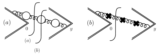
Figure 2: (a) Cut diagrams with fermion loops. (b) Non-vanishing contribution with no cut fermion loop. The crosses denote counterterm insertions.

and $\beta_{0}^{f}=N_{f}/(6\pi)$. As in lowest order, the only non-vanishing type of diagram is that shown in Fig. 2a and the symmetric one. The cuts in this diagram proportional to $\delta(k^{2})$ all vanish except for the diagram with no fermion loop, since with $k^{2}=0$ the fermion loop is given by an integral without scale. The diagram with no loop will be added later. The non-zero cuts are those proportional to $\Theta(k^{2})$, labelled (b), when a fermion loop is cut. The corresponding imaginary part of the effective gluon propagator with an arbitrary number of fermion loops is

$$\frac{g_{\mu\nu}}{k^{2}}\sum_{n=1}^{\infty}\alpha_{s}^{n}\left(-\frac{\beta_{0}^{f}}{\epsilon}\right)^{n}L(\epsilon)^{n}\left(\frac{k^{2}}{\mu^{2}e^{\gamma_{E}}}\right)^{-n\epsilon}\sin\pi(-n\epsilon)\,.$$ (5.14)

The $k_{\mu}k_{\nu}$-terms can be dropped due to gauge invariance (they are cancelled by diagrams not shown). A short calculation gives for the sum of all diagrams with cut fermion loops

$$\frac{C_{F}\alpha_{s}}{\pi}\frac{2}{1-z}\sum_{n=1}^{\infty}\alpha_{s}^{n}\frac{(\beta_{0}^{f})^{n}}{(n+1)(-\epsilon)^{n+1}}\,G(-\epsilon,-(n+1)\epsilon)\,,$$ (5.15)

$$G(-\epsilon,-(n+1)\epsilon)\equiv L(\epsilon)^{n}\left(\frac{Q^{2}}{4\mu^{2}e^{\gamma_{E}}}(1-z)^{2}\right)^{-(n+1)\epsilon}\frac{\sqrt{\pi}}{\Gamma(1/2-(n+1)\epsilon)\Gamma(1+n\epsilon)}\,.$$

When we add the counterterms for the fermion loops, a non-vanishing contribution requires again that at least one fermion loop is cut, except when all fermion loops are replaced by counterterms as in Fig. 2b. The second contribution will be added shortly. Accounting for the first one, the previous expression is modified to [25]

$$\frac{C_{F}\alpha_{s}}{\pi}\frac{2}{1-z}\sum_{n=1}^{\infty}\alpha_{s}^{n}(\beta_{0}^{f})^{n}\sum_{k=0}^{n-1}\frac{1}{(-\epsilon)^{n+1}}\frac{(-1)^{k}}{n+1-k}\left(\!\!\begin{array}[]{c}n\\ k\end{array}\!\!\right)G(-\epsilon,-(n+1-k)\epsilon)\,.$$ (5.16)

Next we note that the remaining contribution from the lowest order diagram together with the ones where all fermion loops are replaced by counterterms is simply

$$W^{\rm(1)}_{\rm DY}(z,\alpha_{s})\,\frac{1}{1-\alpha_{s}\beta_{0}^{f}/\epsilon}$$ (5.17)

with $W^{\rm(1)}_{\rm DY}(z,\alpha_{s})$ as in eq. (5.12). Adding this term amounts to extending the sum over $n$ to 0 and the sum over $k$ to $n$ in eq. (5.16).

Eq. (5.16) contains poles $\alpha_{s}^{n}/\epsilon^{n+1}$, but an additional $1/\epsilon$ is in fact present as seen by introducing +-distributions. At this point it is convenient to pass to moments, before we take the final overall subtractions. The integral over $z$ is trivial and we obtain

$$W_{\rm DY}(N,\alpha_{s})=2\frac{C_{F}\alpha_{s}}{\pi}\sum_{n=0}^{\infty}\alpha_{s}^{n}(\beta_{0}^{f})^{n}\sum_{k=0}^{n}\frac{1}{(-\epsilon)^{n+2}}\frac{(-1)^{k}}{(n+1-k)^{2}}\left(\!\!\begin{array}[]{c}n\\ k\end{array}\!\!\right)H(-\epsilon,-(n+1-k)\epsilon)\,,$$ (5.18)

$$H(\epsilon,s)=\left[L(-\epsilon)\right]^{s/\epsilon-1}\left(\frac{Q^{2}}{\mu^{2}e^{\gamma_{E}}}\right)^{s}\frac{\Gamma(N)\Gamma(1+s)}{2\Gamma(N+2s)\Gamma(1-s+\epsilon)}\,.$$ (5.19)

Note the signs of the arguments of the function $H$. We introduce expansions

$$H(\epsilon,s)=\sum_{j=0}^{\infty}H_{j}(\epsilon)\,s^{j}\,,\qquad H_{j}(\epsilon)=\sum_{k=0}^{\infty}h_{k}^{[j]}\epsilon^{k}\,.$$ (5.20)

The functions $H_{j}$ are finite for $\epsilon\to 0$ by construction. For later use we collect the expressions

$$H(0,s) = \left(\frac{Q^{2}}{\mu^{2}}e^{-5/3}\right)^{s}\frac{\Gamma(N)\Gamma(1+s)}{2\Gamma(N+2s)\Gamma(1-s)}$$

$$H_{0}(\epsilon) = \frac{1}{2}\frac{\Gamma(4+2\epsilon)}{6\Gamma(1-\epsilon)[\Gamma(2+\epsilon)]^{2}\Gamma(1+\epsilon)}$$ (5.21)

$$H_{1}(\epsilon) = H_{0}(\epsilon)\left\{\frac{1}{\epsilon}\ln L(-\epsilon)+\ln\frac{Q^{2}}{\mu^{2}e^{2\gamma_{E}}}-2\Psi(N)+\Psi(1+\epsilon)\right\}\,.$$

To subtract the overall divergences from eq. (5.18), $H(-\epsilon,-(n+1-k)\epsilon)$ is first expanded in its second variable

$$W_{\rm DY}(N,\alpha_{s}) = 2\frac{C_{F}\alpha_{s}}{\pi}\sum_{n=0}^{\infty}\alpha_{s}^{n}(\beta_{0}^{f})^{n}\sum_{j=0}^{\infty}\frac{H_{j}(-\epsilon)}{(-\epsilon)^{n+2-j}}\sum_{k=0}^{n}(-1)^{k}\left(\!\!\begin{array}[]{c}n\\ k\end{array}\!\!\right)(n+1-k)^{j-2}$$ (5.24)

$$= 2\frac{C_{F}\alpha_{s}}{\pi}\sum_{n=0}^{\infty}\alpha_{s}^{n}(\beta_{0}^{f})^{n}\Bigg{\{}\frac{(-1)^{n}}{n+1}(\Psi(n+2)-\Psi(1))\frac{1}{(-\epsilon)^{n+1}}H_{0}(-\epsilon)$$

$$+\,\frac{(-1)^{n}}{n+1}\frac{1}{(-\epsilon)^{n+1}}H_{1}(-\epsilon)+n!\,H_{n+2}(0)+{\cal O}(\epsilon)\Bigg{\}}\,.$$

To arrive at the second line we use

$$\sum_{k=0}^{n}(-1)^{k}\left(\!\!\begin{array}[]{c}n\\ k\end{array}\!\!\right)(n+1-k)^{j-2}=\left\{\,\,\,\begin{array}[]{ll}(-1)^{n}/(n+1)(\Psi(n+2)-\Psi(1))&j=0\\ (-1)^{n}/(n+1)&j=1\\ 0&j=2,\ldots,n+1\\ n!&j=n+2\end{array}\right.$$ (5.26)

Minimal subtraction of the pole part in $\epsilon$ gives the final expression for the $\overline{\rm MS}$-renormalized Wilson line with an infinite number of fermion loops:

$$W_{\rm DY}(N,\alpha_{s}) = 2\frac{C_{F}\alpha_{s}}{\pi}\sum_{n=0}^{\infty}\alpha_{s}^{n}(\beta_{0}^{f})^{n}\bigg{\{}\frac{(-1)^{n}}{n+1}(\Psi(n+2)-\Psi(1))\,h^{[0]}_{n+2}$$ (5.27)

$$\hskip 56.9055pt+\,\frac{(-1)^{n}}{n+1}\,h^{[1]}_{n+1}+n!\,H_{n+2}(0)\bigg{\}}$$

Note that the result contains two terms related to the ‘anomalous dimension functions’ $H_{0}$ and $H_{1}$, that appeared as coefficients of the $1/\epsilon^{n+2}$ and $1/\epsilon^{n+1}$ pieces before, and a ‘finite term’ with coefficient $n!$. It is instructive to take the Borel transform of the above series. We then obtain

$$B\left[W_{\rm DY}\right](N,u)=2\frac{C_{F}}{\pi}\left[\frac{H(0,-u)-H_{0}(0)+u\tilde{H}_{1}(u)}{u^{2}}+\frac{1}{u}\frac{d}{du}\int\limits_{0}^{1}dx\frac{x\tilde{H}_{0}(u)-\tilde{H}_{0}(xu)}{x(1-x)}\right]\,,$$ (5.28)

where $\tilde{H}_{j}(u)\equiv\sum_{n=0}h_{n}^{[j]}u^{n}/n!$ is essentially the Borel transform of $H_{j}(\epsilon)$, cf. eq. (5.20). With the explicit expression for $H(0,-u)$ from eq. (5.3), we find that this term above coincides with the large-$N$ limit of the Borel transform of the full Drell-Yan cross section in eq. (5.11), up to corrections $1/N$ that have been neglected in both cases. There it was understood that the double pole at $u=0$ would be cancelled by virtual corrections and distribution functions, but eq. (5.11) provided the leading power corrections $(N\Lambda_{\rm QCD}/Q)^{2k}$ ($k=1,\ldots$). In the present case the divergences are subtracted by the functions $H_{0}$ and $H_{1}$. These additional terms are analytic in $u$ (as expected for anomalous dimensions in minimal subtraction schemes), so that indeed the Wilson line operators incorporate the leading power corrections (with the largest positive power of $N$) to the hard Drell-Yan cross section. In particular, no power correction of order $1/Q$ appears. Another important observation is that only the function $H_{0}$ is related to the most singular pole in $\epsilon$, which comes from soft and collinear emission. While $H_{0}$ will therefore be related to the universal cusp (eikonal) anomalous dimension, all conclusions on power corrections follow from $H(0,-u)$ which is process-specific (that is, depends on the Wilson contour and not its cusps alone).

5.4 Evolution equation and resummation

Since eq. (5.27) is exact in the single-chain approximation, it must satisfy the RG equation (5.4) to the same accuracy, that is with $\beta(\alpha_{s})=\beta_{0}\alpha_{s}^{2}$ and $\ln[1+W_{\rm DY}]$ equivalent to $W_{\rm DY}$, see the discussion in Sect. 2.3. (The unity under the logarithm is the tree-level contribution $W_{\rm DY}^{(0)}=1$.) Using the explicit expression in eq. (5.28) we get

$$\left(\mu^{2}\frac{\partial}{\partial\mu^{2}}+\beta_{0}\alpha_{s}^{2}\frac{\partial}{\partial\alpha_{s}}\right)\,\ln W_{\rm DY}=-\frac{1}{\beta_{0}}\int_{0}^{\infty}du\,e^{u/(\beta_{0}\alpha_{s})}\left[\mu^{2}\frac{\partial}{\partial\mu^{2}}-u\right]B[W_{\rm DY}](N,u)$$

$$\hskip 56.9055pt=\frac{2C_{F}\alpha_{s}}{\pi}\left\{-H_{1}(a_{s})-\sum_{n=0}^{\infty}a_{s}^{n}h^{[0]}_{n+1}[\Psi(n+2)-\Psi(1)]\right\}$$

$$\hskip 56.9055pt=\frac{2C_{F}\alpha_{s}}{\pi}\left\{-H_{1}(a_{s})-\frac{1}{a_{s}}\int_{0}^{1}dx\,\frac{H_{0}(a_{s})-H_{0}(xa_{s})}{1-x}\right\}\,,$$ (5.29)

where we have restored the full non-abelian $\beta_{0}=-(11-2/3N_{f})/(4\pi)$ and introduced

$$a_{s}=-\beta_{0}\alpha_{s}\,.$$ (5.30)

In the large-$N$ limit we expect to find a term logarithmic in $N$, multiplied by the cusp anomalous dimension. From the explicit expression for $H_{1}$ we get indeed

$$-\frac{2C_{F}\alpha_{s}}{\pi}H_{1}(a_{s})=\frac{C_{F}\alpha_{s}}{\pi}\frac{\Gamma(4+2a_{s})}{6\Gamma(1-a_{s})[\Gamma(2+a_{s})]^{2}\Gamma(1+a_{s})}\cdot 2\ln\frac{N\mu}{N_{0}Q}$$ (5.31)

with $N_{0}=e^{-\gamma_{E}}$ and omitting terms without $\ln N$. Thus

$$\Gamma_{\rm cusp}(\alpha_{s}) = 2\frac{C_{F}\alpha_{s}}{\pi}H_{0}(a_{s})=\frac{C_{F}\alpha_{s}}{\pi}\frac{\Gamma(4+2a_{s})}{6\Gamma(1-a_{s})[\Gamma(2+a_{s})]^{2}\Gamma(1+a_{s})}$$ (5.32)

$$= \frac{C_{F}\alpha_{s}}{\pi}\left\{1-\frac{5}{3}a_{s}-\frac{1}{3}a_{s}^{2}+2.0708a_{s}^{3}-1.0932a_{s}^{4}+\ldots\right\}\,,$$

in agreement with the known two-loop result (keeping the leading $N_{f}$-term only) [15, 26]. We verify coincidence with the direct calculation in Appendix A.

The remaining terms in eq. (5.4) (up to $1/N$-corrections, which are consistently neglected) give $\Gamma_{\rm DY}(\alpha_{s})$:

$$\Gamma_{\rm DY}(\alpha_{s}) = 2\frac{C_{F}\alpha_{s}}{\pi}\left\{H_{0}(a_{s})\left[-\frac{1}{a_{s}}\ln L(-a_{s})-\Psi(1+a_{s})\right]-\sum_{n=0}^{\infty}a_{s}^{n}h^{[0]}_{n+1}[\Psi(n+2)-\Psi(1)]\right\}$$ (5.33)

$$= 2\frac{C_{F}\alpha_{s}}{\pi}\left\{\left(\frac{7}{9}-\frac{\pi^{2}}{24}\right)a_{s}-0.08547a_{s}^{2}-0.1537a_{s}^{3}+0.4951a_{s}^{4}+\ldots\right\}$$

Note that $\Gamma_{\rm DY}(\alpha_{s})$ starts from second order in $\alpha_{s}$ [14]. Eq. (5.28) can now be written as

$$B[W_{\rm DY}](N,u)=B[W^{\rm real}](N,u)\left(\frac{\mu^{2}}{Q^{2}}\right)^{u}-\frac{1}{u^{2}}B[\Gamma_{\rm cusp}](u)\left[1+2u\ln\frac{N\mu}{N_{0}Q}\right]-\frac{1}{u}B[\Gamma_{\rm DY}](u)$$ (5.34)

The first term on the right hand side gives the unrenormalized Borel transform, which coincides with $B[W^{\rm real}]$, eq. (5.11), and the two other terms are the subtractions, necessary for finiteness at $u=0$.

The anomalous dimensions, eq. (5.32) and (5.33), have finite radius of convergence (in the $\overline{\rm MS}$ scheme) and their Borel transforms are entire functions. At $u=1/2$ they are non-zero. We conclude that none of the terms in the evolution equation for the Wilson line, eq. (5.4), contains renormalons, and neither does the particular solution corresponding to the integral in eq. (5.5). (Let us insist again that one must stay in the perturbative domain $N<Q/\Lambda_{\rm QCD}$). In the present formalism, all IR renormalons to resummed cross sections are introduced through the initial condition (or solution to the homogeneous equation) for the evolution of the Wilson line. The initial condition can be determined by comparison with exact calculation (in the single-chain approximation),

$$B[X](N,u)=B[W^{\rm real}](N,u)-\frac{1}{u^{2}}\left(\frac{N}{N_{0}}\right)^{2u}\left[B[\Gamma_{\rm cusp}](u)+uB[\Gamma_{\rm DY}](u)\right]\,,$$ (5.35)

and consequently, the renormalons in the initial condition are exactly those in eq. (5.28). We find once more that the dominant IR renormalon requires non-perturbative contributiuons only at order $N^{2}\Lambda_{\rm QCD}^{2}/Q^{2}$. All terms in eq. (5.35) have the same $N$-dependence proportional to $N^{2u}$. This verifies that the initial condition is a function only of $\alpha_{s}(QN_{0}/N)$. Indeed, using eq. (2.12) we get

$$B[X(\alpha_{s}(QN_{0}/N)](u)=\left(\frac{N}{N_{0}}\right)^{2u}B[X(\alpha_{s}(Q))](u)\,.$$ (5.36)

It remains to clarify the origin of apparent linear power corrections to the resummed cross section in the form of eq. (2.2). The difference with eq. (5.5) lies in the choice of the inhomogeneous term in the solution to the evolution equation as

$$\ln W_{\rm DY}\!\left(\frac{\mu^{2}N^{2}}{Q^{2}N_{0}^{2}},\alpha_{s}(\mu)\right) = X^{\prime}(\alpha_{s}(QN_{0}/N))\,-2\int\limits_{0}^{1}dz\frac{z^{N-1}-1}{1-z}\Bigg{[}\int\limits_{(1-z)^{2}Q^{2}}^{\mu^{2}}\frac{dk_{t}^{2}}{k_{t}^{2}}\,\Gamma_{\rm cusp}(\alpha_{s}(k_{t})$$ (5.37)

$$\hskip 85.35826pt+\,\Gamma_{\rm DY}(\alpha_{s}((1-z)Q)\Bigg{]}\,.$$

A simple calculation (as in Sect. 2.2) yields for the difference of Borel transforms of the integrals in eq. (5.5) and eq. (5.37)

$$\left(\frac{N}{N_{0}}\right)^{2u}\left(N_{0}^{-2u}\Gamma(1-2u)-1\right)\frac{1}{2u^{2}}\left[B[\Gamma_{\rm cusp}](u)+uB[\Gamma_{\rm DY}](u)\right]\,.$$ (5.38)

This difference has to be compensated by a change in the solution of the homogeneous RG equation, which now becomes,

$$B[X^{\prime}](N,u)=B[W^{\rm real}](N,u)-\frac{1}{u^{2}}\left(\frac{N}{N_{0}}\right)^{2u}N_{0}^{-2u}\Gamma(1-2u)\left[B[\Gamma_{\rm cusp}](u)+uB[\Gamma_{\rm DY}](u)\right]\,.$$ (5.39)

Comparing with eq. (5.35), we see that this change involves singular terms at $u=1/2$. Because of the $\Gamma(1-2u)$, both, the Borel transform of $X^{\prime}$ and of the integral in eq. (5.37) have IR renormalon poles at $u=1/2$ (corresponding to $1/Q$) with residue proportional to $N$, but opposite sign, so that in the sum the singularity cancels. In the Borel transform of the integral in eq. (5.37) the pole is present through the functions $\Delta_{1}$ and $\Delta_{3}$, introduced in Sect. 2.2, and is cancelled in this representation by an explicit pole in $X^{\prime}$. If, to return to the standard representation, the initial condition contribution $X^{\prime}$ is eliminated by the redefinitions of eq. (5.1), this cancellation persists in the exponent. Indeed, for the functions $A$ and $C$ in eq. (2.2) we get

$$B[A](u) = B[\Gamma_{\rm cusp}](u)$$

$$-\frac{1}{2}B[C](u) = B[\Gamma_{\rm DY}](u)+u\left(\frac{N_{0}}{N}\right)^{2u}\frac{N_{0}^{2u}}{\Gamma(1-2u)}B[X](N,u)$$

$$= uB[W^{\rm real}](N,u)\left(\frac{N_{0}}{N}\right)^{2u}\frac{N_{0}^{2u}}{\Gamma(1-2u)}-\frac{1}{u}B[\Gamma_{\rm cusp}](u)\,,$$

so that

$$2B[A](u)-uB[C](u)=\frac{2N_{0}^{2u}}{\Gamma(1-2u)}u^{2}\left(\frac{N_{0}}{N}\right)^{2u}B[W^{\rm real}](N,u)\,.$$ (5.41)

Due to the Gamma-function in the denominator, this combination has a zero at $u=1/2$, independent of the particular form of $B[W^{\rm real}](N,u)$ (unless it is singular, which is not the case, at least in the single-chain approximation, see eq. (5.28)). Note that all contributions from the anomalous dimensions $\Gamma_{\rm cusp}$ and $\Gamma_{\rm DY}$ disappear.

We conclude that the cancellation of scenario B in Sect. 2.2 does occur and no indication for physical ‘higher twist’ corrections of order $1/Q$ remains. The cancellation of such corrections with the remainder $R$ as in mechanism C could only have taken place, if the soft approximation had accounted correctly for the leading-$N$ behaviour only to logarithmic, but not to power-like accuracy. This is not the case. As noted before (and expected), $W_{\rm DY}$ computed in the eikonal approximation (Wilson line) reproduces those power corrections to the Drell-Yan hard cross section with the largest power in $N$. This suggests that the nonperturbative corrections indicated by renormalons in the Wilson line should exponentiate [5].

6 Discussion and Summary

Let us summarize our investigation of power corrections (alias infrared renormalons) in Drell-Yan production. Our starting observation is that the moments of the resummed hard cross section in the large-$N$ limit can be written in two different ways as

$$\ln\omega_{q\bar{q}}(N,\alpha_{s}(Q)) = -\int\limits_{0}^{1}dz\,\frac{z^{N-1}-1}{1-z}\Bigg{\{}2\int\limits_{Q^{2}(1-z)}^{Q^{2}(1-z)^{2}}\frac{dk_{t}^{2}}{k_{t}^{2}}\,\Gamma_{\rm cusp}(\alpha_{s}(k_{t}))+B(\alpha_{s}(\sqrt{1-z}Q))$$ (6.1)

$$\hskip 56.9055pt+\,C(\alpha_{s}((1-z)Q)\Bigg{\}}+{\cal O}(1)$$

or

$$\ln\omega_{q\bar{q}}(N,\alpha_{s}(Q)) = \int\limits_{0}^{1-e^{-\gamma_{E}}/N}dz\,\frac{1}{1-z}\Bigg{\{}2\int\limits_{Q^{2}(1-z)}^{Q^{2}(1-z)^{2}}\frac{dk_{t}^{2}}{k_{t}^{2}}\,\Gamma_{\rm cusp}(\alpha_{s}(k_{t}))+\tilde{B}(\alpha_{s}(\sqrt{1-z}Q))$$ (6.2)

$$\hskip 56.9055pt+\,\tilde{C}(\alpha_{s}((1-z)Q)\Bigg{\}}+{\cal O}(1)\,.$$

Both forms are equivalent for the purpose of summing large logarithms in $N$, but have apparently different properties as far as sensitivity to the IR Landau pole of the coupling is concerned. When the ‘anomalous dimensions’ $\Gamma_{\rm cusp}$, $B$ etc. are truncated at finite order, the second form has no ambiguity unless $N>Q/\Lambda_{\rm QCD}$, whereas such an ambiguity is present in the first version for any $N$. This apparent conflict is resolved by the analysis of the exponent in Sect. 2.2, which concludes that the correct IR renormalon structure of the exponent can be obtained only, if the anomalous dimensions are also considered to all orders. With respect to eqs. (6.1), (6.2) this means that IR renormalons that are manifest in terms of the integrals over $z$ and $k_{t}$ (the functions $\Delta_{i}$ in Sect. 2.2) in one form can be hidden in the large-order behaviour of the anomalous dimension functions in the other. It is with this observation that we start to differ from previous works, which implicitly assumed that low-order approximations to the anomalous dimensions would be sufficient [4] or the functions $B$ and $C$, which account for gluon emission that is not both, soft and collinear, could be neglected [5, 10].

Already from this conclusion it is evident that, even in the large-$N$ limit the search for power corrections is a problem quite different from resummation of $\ln N$, which can be completed up to a desired order with finite-order approximations to the anomalous dimensions. Although the techniques of soft factorization developed for the purpose of resummation are still effective in isolating those power corrections $(N\Lambda_{\rm QCD}/Q)^{2k}$ with the largest power of $N$, this task requires application of these techniques to all orders in perturbation theory.

We have argued that taking into account these considerations, all corrections of order $1/Q$ cancel in the Drell-Yan cross section and the remaining IR renormalons indicate parametrically smaller power corrections of order $N^{2}\Lambda_{\rm QCD}^{2}/Q^{2}$. The evidence for this cancellation has been collected from two sources: A calculation of the Drell-Yan cross section for any $N$ with finite gluon mass as IR regulator (which by eq. (2.25) can be considered also as a certain approximation to large orders in perturbation theory) does not reveal any IR sensitivity proportional to $\lambda/Q$, even though the phase space in the presence of finite gluon mass is reduced linearly in $\lambda/Q$. The same result has been obtained from implementing the factorization of soft gluon emission in terms of Wilson lines [14] in the approximation of a single chain of vacuum polarization insertions. This approximation may be considered as a model (exact in the unphysical limit of large number of fermions) for the large-order behaviour of the anomalous dimension functions. In this language the absence of $1/Q$-power corrections seems to be most transparent. Renormalizing the Wilson line by minimal subtraction, we find that the anomalous dimensions that enter the renormalization group equation for the Wilson line are analytic for small $\alpha_{s}$ and do not contain IR renormalons. These enter the solution of the evolution equation exclusively through the initial (boundary) condition, which, in general, contains both, perturbative and non-perturbative contributions. As in the exact calculation of the hard Drell-Yan cross section, the power corrections deduced from IR renormalons are of order $N^{2}\Lambda_{\rm QCD}^{2}/Q^{2}$. It is only when this initial condition is absorbed into a redefinition of the functions $B$ and $C$ that IR renormalons enter the exponent. These redefintions are such that the power corrections of order $1/Q$ found from eq. (6.1) [4, 5] are eliminated by an exact zero in the Borel transforms of the corresponding anomalous dimensions.

In Sect. 4 we have seen that the identification of power corrections through IR renormalons or cutoff dependence relies on an exact treatment of soft gluon emission also at large angles, while the collinear approximation can introduce spurious cutoff dependence. It is for this reason that the leading (in $N$) power corrections can not be described by the universal cusp anomalous dimension. In terms of Wilson lines this is seen explicitly by the fact that IR renormalons enter through the initial condition and not as the coefficients of the leading soft and collinear pole in $\epsilon$. We also note that the result on power corrections is not specific to the semi-inclusive limit and applies to all $N$ in the perturbative domain $N<Q/\Lambda_{\rm QCD}$. The analysis of Wilson lines suggests however that, similarly to logarithms in $N$, the power corrections leading in $N$ can also exponentiate.

All explicit calculations of large-order behaviour have been done in the approximation of a single ‘renormalon chain’. If we consider this approximation as an approximation for $\ln\omega_{q\bar{q}}$ rather than the hard cross scetion $\omega_{q\bar{q}}$ as suggested by exponentiation of large logarithms beyond this approximation, then as usual the contributions from several chains are bound to modify the precise numerical coefficient of the $N^{2}\Lambda_{\rm QCD}^{2}/Q^{2}$-terms. To confirm or disprove the absence of $1/Q$ contributions to the Drell-Yan process at the level of two gluon emission would again require an exact treatment of soft gluon emission that goes beyond the usual approximations in treating parton cascades. From the fact that even in the single-chain approximation the IR renormalon structure is sensitive to the large-order behaviour of the anomalous dimensions, we expect this to be a quite challanging problem. Without any further physical evidence to the opposite we find it reasonable to assume that as in other cases (with operator product expansion as a check) [6] multiple chains and more complex diagrams will not modify the power behaviour itself. Still, we recall that the Drell-Yan process may receive power corrections, which can not be seen through IR renormalons, and whose size is not accessible with present theoretical tools.

As pointed out in [8, 9], the question of linear power corrections is of particular importance due to their potential universality, which would allow to treat such power corrections to processes without operator product expansion on a phenomenological level akin to matrix elements of higher dimensional operators in cases with operator product expansion. From this point of view it is interesting to compare the result on power corrections for the Drell-Yan process with those for hadronic event shape variables in $e^{+}e^{-}$-annihilation [21, 7, 8, 9]. In particular, from the point of view of summing large logarithms in $N$ to next-to-leading accuracy, the thrust distribution is closely related to the distribution in $z$ in the Drell-Yan process, $\omega_{q\bar{q}}(z,\alpha_{s}(Q))$, since the large logarithms can be accounted for by the same jet mass distribution [27, 28]. (For a discussion in the present context, see [9, 10].) On the other hand, if we compute the thrust distribution with finite gluon mass to order $\alpha_{s}$, we obtain for the averages

$$\langle 1-T\rangle \sim -8G\,\frac{C_{F}\alpha_{s}}{\pi}\frac{\lambda}{Q}$$

$$\langle T^{N-1}\rangle \sim 8G\,(N-1)\,\frac{C_{F}\alpha_{s}}{\pi}\frac{\lambda}{Q}\,,$$ (6.3)

where $G=\sum_{k=0}(-1)^{k}/(2k+1)^{2}=0.91596\ldots$ is Catalan’s constant. Contrary to the Drell-Yan process, large $1/Q$-corrrections are present for event shapes, in particular for the moments of the thrust-distribution. Some caution is necessary in interpreting the results obtained with finite gluon mass in these cases, since the correspondence with IR renormalons, provided by eq. (2.25) for the DY process, does not hold, because the phase space of the quark pair from gluon splitting in the single chain approximation is not integrated unweighted. We refer to the very recent publication [29], where the relevance of four-parton contributions to $1/Q$-terms is discussed. The difference in $1/Q$-corrections to the DY cross section and thrust reinforces that these corrections can only be identified by a treatment of soft gluon emission at all angles to all orders.

One may speculate on a deeper physical reason for this difference. One possibility is that IR safety of event shape variables is in a certain sense enforced ‘by hand’. Depending on the construction, this can enhance or suppress IR regions in an almost arbitrary way [21]. On the other hand, for the DY process one might be more confident that IR renormalons probe some aspect of the IR dynamics of QCD that eventually might find a rigorous treatment just as higher twist matrix elements in deep inelastic scattering. In this respect it is somewhat comforting that corrections to the DY process appear to be of order $1/Q^{2}$.

The theoretical discussion has been performed in terms of moments. To obtain a prediction for the resummed DY cross section, the inverse Mellin transform has to be taken. Let us note first that there is in fact no compelling reason to evaluate the integrals with running coupling in eqs. (6.1) and (6.2) exactly as long as, as always in practice, only finite-order approximations to the anomalous dimensions are available. To any definite accuracy in the summation of logarithms of $N$, one may expand $\alpha_{s}(k_{t})$ etc. to the required order and perform the integrals term by term. Then the Landau pole in the perturbative running coupling never poses a difficulty. This reflects our previous assertion that the question of power corrections necessarily deals with the all-order behaviour of the anomalous dimensions.

Nevertheless the exact integrals over the running coupling are often kept and the dependence on regulating the Landau pole is then interpreted as the ultimate accuracy that can be achieved without deeper understanding of non-perturbative corrections. From our analysis we conclude that such a treatment has to be interpreted with care, since the failure to include the anomalous dimensions to all orders may pretend artificially large regularization dependence. From this point of view, the construction of the inverse Mellin transform starting from eq. (6.2) is preferred compared to eq. (6.1), which was used in [4], since spurious large corrections of order $N\Lambda_{\rm QCD}/Q$ do not appear. We find confirmation for this suggestion from the analysis of [30], where comparison of the resummed cross section based on eq. (6.1) [4, 18] with data requires to fit rather large corrections proportional to $N\Lambda_{\rm QCD}/Q$, whose main effect is to reduce the effect of resummation.

The phenomenological implications could pertain to processes other than Drell-Yan. For instance, a resummation similar to the Drell-Yan case has also been completed for the top production cross section (where in addition large corrections from gluon-gluon fusion have to be considered) [31]. It might be worthwhile to investigate the rather large cutoff dependence reported in the light of the results presented in this paper, especially since the cutoff was chosen much larger than $\Lambda_{\rm QCD}$. An improvement of the theoretical Standard Model prediction is crucial to unravel potential anomalous couplings of the top quark in its production cross section.

We conclude that further explorations of power corrections, both theoretical and phenomenological, are expected to provide further insight into the workings of QCD and will help understanding the limitations of perturbative QCD in describing data for hadronic observables.

Acknowledgements. M. B. thanks G. Marchesini and I. Z. Rothstein and V. B. thanks G. P. Korchemsky for helpful discussions and critical reading of the manuscript. Both authors are grateful to the members of the CERN Theory group for their hospitality, when part of this work was done. M. B. is supported by the Alexander von Humboldt-foundation.

Appendix A

In this appendix we sketch a simple derivation of the cusp anomalous dimension to all orders in the $1/N_{f}$-approximation (single-chain approximation). In lowest order, the cusp anomalous dimension is given by the $1/\epsilon$-pole in the diagram shown in Fig. 3. In higher orders we adopt dimensional regularization with minimal subtraction. As shown in [19] the series in the $1/N_{f}$-approximation can be extracted from the large-$\lambda$ behaviour of the diagram, when evaluated with a gluon of mass $\lambda$. A straightforward calculation gives

$$-ig_{s}^{2}C_{F}\mu^{2\epsilon}\int\frac{d^{d}k}{(2\pi)^{d}}\frac{p_{1}\cdot p_{2}}{(k^{2}-\lambda^{2})\,p_{1}\cdot k\,p_{2}\cdot k}=-\frac{C_{F}\alpha_{s}}{2\pi}\frac{\Gamma(1+\epsilon)}{\epsilon}\left(\frac{\lambda^{2}}{4\pi\mu^{2}}\right)^{-\epsilon}\,\gamma\,\mbox{coth}\,\gamma\,,$$ (A.1)

where $\mbox{cosh}\,\gamma=(p_{1}\cdot p_{2})/\sqrt{p_{1}^{2}p_{2}^{2}}$ is the Minkowskian cusp angle [26]. The cusp anomalous dimension can be read off the coefficient of $1/\epsilon\,(\lambda^{2}/\mu^{2})^{-\epsilon}$ [19] (Appendix A) and we obtain (adding self-energy contributions, which result in $\gamma\,\mbox{coth}\,\gamma\to\gamma\,\mbox{coth}\,\gamma-1$)

$$\Gamma_{\rm cusp}(\alpha_{s}) = \frac{C_{F}\alpha_{s}}{\pi}\,\frac{\Gamma(4-2\beta_{0}\alpha_{s})}{6\Gamma(2-\beta_{0}\alpha_{s})^{2}\Gamma(1-\beta_{0}\alpha_{s})\Gamma(1+\beta_{0}\alpha_{s})}\,(\gamma\,\mbox{coth}\,\gamma-1)$$ (A.2)

$$= \left[C_{F}\frac{\alpha_{s}}{\pi}-\frac{5}{18}C_{F}N_{f}\left(\frac{\alpha_{s}}{\pi}\right)^{2}-\frac{1}{108}C_{F}N_{f}^{2}\left(\frac{\alpha_{s}}{\pi}\right)^{3}+\ldots\right](\gamma\,\mbox{coth}\,\gamma-1)\,,$$

where $\beta_{0}=N_{f}/(6\pi)$. The second order coefficient is in agreement with the $N_{f}$-term of the complete two-loop result [15, 26]. The above series gives the term with the largest power of $N_{f}$ to all orders.

3

Figure 3: Diagram for the cusp anomalous dimension. The double lines denote a Wilson line with cusp (alternatively, they can be interpreted as eikonal propagators).

Appendix B

The different power corrections to the Drell-Yan cross section and averages of thrust can be reduced to a few elementary integrals. First we write for the moments

$$\langle X^{N-1}\rangle=\langle 1\rangle-(N-1)\langle 1-X\rangle+\ldots\,,$$ (B.1)

where $X=T$ (thrust) or $X=z$ (Drell-Yan) and the brackets denote averaging with the corresponding distribution in $T$ or $z$. For the Drell-Yan cross section it is given by eq. (3.7). The omitted terms do not contribute to terms of order $\lambda/Q$, since each power of $1-X$ suppresses the region of phase space $X\to 1$ where linear terms can arise. One can show that $\langle 1\rangle$ is free from such terms in both cases, so that the problem reduces to the average of $1-X$. This average receives no virtual corrections and is free from soft divergences.

For the Drell-Yan cross section, we use the new variable $y=1-z-\xi z$ ($\xi=\lambda^{2}/Q^{2}$). Neglecting all terms that can not give rise to $\sqrt{\xi}$ in the expansion for small $\xi$, we find

$$\langle 1-z\rangle\sim 4\frac{C_{F}\alpha_{s}}{\pi}\int\limits_{\sqrt{\xi}}^{\epsilon}dy\,\ln\frac{y+\sqrt{y^{2}-\xi}}{y-\sqrt{y^{2}-\xi}}\sim 4\frac{C_{F}\alpha_{s}}{\pi}\left[\epsilon\ln\xi+0\cdot\sqrt{\xi}+\ldots\right]\,,$$ (B.2)

where $\epsilon$ is an arbitrary cutoff that does not affect linear terms in $\lambda$ and ‘$\sim$’ means that the expression is accurate to linear terms. Although the lower limit of the integral is $\sqrt{\xi}$, its expansion does not contain such terms. The logarithm of $\xi$ is due to the fact that the partonic cross section is not collinear safe. It is subtracted by the parton distribution function, which does not introduce linear terms either (Sect. 3).

In case of thrust it is convenient to switch from the energy fractions $x_{1}$ and $x_{2}$ of quark and anti-quark as integration variables to $y=1-1/2\,(x_{1}+x_{2})$ and $x=(x_{1}-x_{2})/2$. We then find after integration over $x$

$$\langle 1-T\rangle \sim 2\frac{C_{F}\alpha_{s}}{\pi}\int\limits_{\sqrt{\xi}}^{\epsilon}dy\,\left[\left(1-\frac{\xi}{y^{2}}\right)^{1/2}\ln\frac{y+\sqrt{y^{2}-\xi}}{y-\sqrt{y^{2}-\xi}}+\ln\frac{\xi}{y^{2}}\right]$$ (B.3)

$$\sim 2\frac{C_{F}\alpha_{s}}{\pi}\left[0\cdot\ln\xi-4G\sqrt{\xi}+\ldots\right]\,,$$

where $G=0.91596\ldots$ is Catalan’s constant. The additional logarithm in the integrand as compared to the Drell-Yan case eliminates the logarithm of $\xi$ as required by collinear safety of thrust, but introduces a (n additional) linear correction in $\lambda/Q$. If the $\xi$-dependence of the normalization $\sum_{i}|\vec{p}_{i}|$ of thrust is neglected, the square root in front of the logarithm is absent and we obtain the different result of [7].

References

- [1] See J. C. Collins, D. E. Soper and G. Sterman, in ‘Perturbative Quantum Chromodynamics’, ed. A. H. Mueller (World Scientific, Singapore, 1989), and references therein.
- [2] G. Sterman, Nucl. Phys. B281 (1987) 310
- [3] S. Catani and L. Trentadue, Nucl. Phys. B327 (1989) 323
- [4] H. Contopanagos and G. Sterman, Nucl. Phys. B419 (1994) 77
- [5] G. P. Korchemsky and G. Sterman, Nucl. Phys. B437 (1995) 415
- [6] G. ’t Hooft, in ‘The Whys of Subnuclear Physics’, Proc. Int. School, Erice, 1977, ed. A. Zichichi (Plenum, New York, 1978). For overviews of some classical applications and further references see V. I. Zakharov, Nucl. Phys. B385 (1992) 452, A. H. Mueller, in ‘QCD – Twenty Years Later’, Proc. Int. Conf., Aachen, 1992, ed. P. Zerwas and H. Kastrup, Vol. 1 (World Scientific, Singapore, 1993), Sect. 2 of [25] and V. M. Braun, talk presented at ‘QCD and High Energy Hadronic Interactions’, Moriond, 1995, to appear in the proceedings [hep-ph/9505317]
- [7] B. R. Webber, Phys. Lett. B339 (1994) 148
- [8] Yu. L. Dokshitser and B. R. Webber, Cavendish report CAVENDISH-HEP-94-16 (1995) [hep-ph/9504232]
- [9] R. Akhoury and V. I. Zakharov, Saclay report, SPhT Saclay T95/043 (1995) [hep-ph/9504248]
- [10] G. P. Korchemsky and G. Sterman, talk presented at ‘QCD and High Energy Hadronic Interactions’, Moriond, 1995, to appear in the proceedings, SUNY preprint ITP-SB-95-17 [hep-ph/9505391]
- [11] I. Bigi et al., Phys. Rev. D50 (1994) 2234
- [12] M. Beneke, V. M. Braun and V. I. Zakharov, Phys. Rev. Lett. 73 (1994) 3058
- [13] M. Beneke, Nucl. Phys. (Proc. Suppl.) 39B (1995) 405
- [14] G. P. Korchemsky and G. Marchesini, Nucl. Phys. B406 (1993) 225; Phys. Lett. B313 (1993) 433
- [15] J. Kodaira and L. Trentadue, Phys. Lett. B112 (1982) 66
- [16] L. Magnea, Nucl. Phys. B349 (1991) 703
- [17] S. Catani and L. Trentadue, Nucl. Phys. B353 (1991) 183
- [18] L. Alvero and H. Contopanagos, Nucl. Phys. B436 (1995) 184
- [19] P. Ball, M. Beneke and V. M. Braun, CERN report CERN-TH/95-26 (1995) [hep-ph/9502300]
- [20] M. Beneke, Nucl. Phys. B405 (1993) 424 and references in [19]
- [21] A. V. Manohar and M. B. Wise, Phys. Lett. B344 (1995) 407
- [22] D. Amati et al., Nucl. Phys. B173 (1980) 429
- [23] M. Beneke and V. M. Braun, Phys. Lett. B348 (1995) 513
- [24] G. Altarelli, R. K. Ellis and G. Martinelli, Nucl. Phys. B143 (1978) 521 [Erratum: ibid., B146 (1978) 544]; J. Kubar-André and F. E. Paige, Phys. Rev. D19 (1979) 221
- [25] M. Beneke and V. M. Braun, Nucl. Phys. B426 (1994) 301
- [26] G. P. Korchemsky and A. V. Radyushkin, Nucl. Phys. B283 (1987) 342
- [27] S. Catani, B. R. Webber and G. Marchesini, Nucl. Phys. B349 (1991) 635
- [28] S. Catani, L. Trentadue, G. Turnock and B. R. Webber, Nucl. Phys. B407 (1993) 3
- [29] P. Nason and M. H. Seymour, CERN preprint CERN-TH/95-150 [hep-ph/9506317]
- [30] L. Alvero, SUNY preprint ITP-SB-94-67 (1994) [hep-ph/9412335]
- [31] E. Laenen, J. Smith and W. L. van Neerven, Nucl. Phys. B369 (1992) 543; Phys. Lett. B321 (1994) 254