FERMILAB-Pub-95/127-T

DTP/95/52

The Determination of $\alpha_{S}$ at Hadron Colliders

W. T. Giele
Fermi National Accelerator Laboratory, P. O. Box 500,
Batavia, IL 60510, U.S.A.

E. W. N.  Glover
Physics Department, University of Durham,
Durham DH1 3LE, England

and

J.  Yu
Department of Physics and Astronomy, University of Rochester

Rochester, NY 14627, U.S.A.

Hadron colliders offer a unique opportunity

to test perturbative QCD because, rather than

producing events at a specific beam energy, the dynamics

of the hard scattering is probed simultaneously at a wide

range of momentum transfers.

This makes the determination of $\alpha_{S}$

and the parton density functions (PDF) at hadron colliders particularly interesting.

In this paper we restrict ourselves to extracting $\alpha_{S}$ for a given PDF at a scale

which is directly related

to the transverse energy produced in the collision. As an example, we focus on

the single jet inclusive transverse energy

distribution and use the published ’88-’89 CDF data with an integrated luminosity of 4.2 pb^-1. The evolution of the coupling constant over a wide range of scales (from 30 GeV to 500 GeV) is clearly shown and

is in agreement with the QCD expectation. The data to be obtained in the current Tevatron run (expected to be well in excess 100 pb^-1 for both the CDF

and DØ experiments) will significantly decrease the experimental errors.

1 Introduction

Hadronic collisions at the Fermilab TEVATRON

offer excellent opportunities to study QCD over a

broad range of momentum transfers ranging from a few GeV in the transverse

momentum distribution of the $Z$ boson up to almost half of the beam energy in the single jet

inclusive transverse energy distribution. While the experiments at LEP and HERA have

set well defined goals for QCD studies,

hadron colliders tend to be thought of as discovery machines probing the high energy frontier. For example, at Fermilab, the major effort has been concentrated on the study of the Top Quark and $W$-mass measurements.

In this paper, we try to redress this imbalance and outline a possible goal for QCD studies at hadron colliders.

Achieving this goal will give both a rigorous

test of QCD and a reduction of the experimental systematic errors in the other studies at Fermilab.

One possible goal of QCD studies at the Main Injector [1] is to use the QCD data set to determine the input parameters of the theory,

in other words, $\alpha_{S}$ and the parton density functions (PDF’s),

without input from other experiments. This should also allow the determination of the gauge symmetry responsible for the strong interactions thereby extending similar measurements at LEP [2].

In order to achieve this goal, we need to make several intermediate steps to identify problems in both

experiments and theory. The run 1A and 1B data can be used to

gain experience in how to analyze the data and to identify those distributions which can be measured accurately and calculated reliably. We will break the program into four steps with each phase contributing to a better understanding of QCD at hadron colliders.

In the first phase we use the PDF’s obtained from global analyses [3, 4, 5, 6] and the associated $\mbox{$\alpha_{S}$}(M_{Z})$ as input parameters.

Then by comparing data to theory we

can identify those cross sections which are most sensitive to the input parameters.

Using run 1A data it has become clear that certain distributions will be better than others in determining the parton density functions and $\alpha_{S}$. For example, the parton density functions can be constrained from di-jet data using angular correlations [7], the same-side to opposite-side ratio [8, 9, 10] and via the triply differential cross section [11, 12, 13, 14, 15] while the strong coupling can be determined from vector boson production at large transverse momentum [16, 17, 18].

In the second phase we will assume a given PDF set as being correct and extract $\alpha_{S}$. Measuring $\alpha_{S}$ at a hadron collider is rather different than measuring $\alpha_{S}$ at LEP with the most important difference being the fact that one can

measure $\alpha_{S}$ from momentum transfers as low as a few

GeV all the way up to 500 GeV simultaneously and with high statistics [15]. In this paper we will use the

one-jet inclusive transverse energy distribution

measured from the ’88-’89 CDF data with an integrated luminosity of 4.2 $\mbox{pb}^{-1}$

to illustrate this method. The analysis can be repeated for the current CDF and DØ data sets

increasing the integrated luminosity to well over 100 $\mbox{pb}^{-1}$. These increased statistics

will have a major impact on both the statistical and systematic error

relative to the ’88-’89 data set.

The results in this paper are therefore just

an illustration of the method and no detailed effort has been made to determine the

experimental systematic errors thoroughly. This would require detailed knowledge of the

correlation matrix for the systematic error which is not readily available. While the value of $\alpha_{S}$ extracted in

this way cannot be considered on the same footing as that measured at LEP because the PDF’s themselves are dependent on $\alpha_{S}$, this measurement will nevertheless provide valuable information.

For example, the extracted $\alpha_{S}$ must be consistent with the $\alpha_{S}$ used in the PDF, or else the data is incompatible with

this particular set. If one finds that the extracted $\alpha_{S}$ is compatible with the PDF the measurement gives an additional constraint on the PDF at large $x$ and $Q^{2}$. Further, one can also study the evolution of $\alpha_{S}$ for a wide range of momentum transfers.

In the third phase we determine both

the PDF’s and $\alpha_{S}$ simultaneously using the triply differential di-jet inclusive distributions [8, 11, 12], possibly including flavor tagging, yielding an $\alpha_{S}$

that is completely independent of the DIS data set.

In principle the measurement is very simple,

the parton fractions are determined by summing over the rapidity weighted

transverse momenta of the particles

produced by the hard scattering,

$x_{1,2}=(\sum_{i}E_{T}^{i}e^{\pm\eta_{i}})/\sqrt{S}$ [13, 14]. However, since it is impossible to measure and identify all the

particles associated with the hard scattering, we are forced to rely on

higher order calculations to estimate the unobserved

radiation. It might therefore be prudent to separate

this phase into two steps by first determining the distribution of gluons in the

proton and assuming the distribution of charged partons is determined by the DIS data set. The reason for this is that in deep inelastic scattering the virtual photon directly probes the charged parton distributions. The effects of the gluon distribution enter first

at next-to-leading order and cause, for example,

scaling violations in

the slope of $F_{2}$. On the other hand, in hadron colliders,

the gluon density enters at lowest order

and a more direct measurement should be possible. For example, by using the triply differential di-jet data one probes the gluon distribution directly with essentially unlimited statistics. After the gluon distribution has been successfully extracted in this manner, one can include the triply differential $V+$ jet data

(where $V=W,Z,\gamma$) to extract the charged PDF’s. A succesful determination of both $\alpha_{S}$ and the

PDF’s from the hadronic data set over a wide range of momentum transfers would be an important

test of QCD and its consistent description using perturbative QCD. The measured PDF’s and $\alpha_{S}$ can directly be used in

other physics analyses at hadron colliders thereby reducing the experimental systematic uncertainties considerably.

After completing the program outlined above, one can then test QCD and

the gauge group responsible for the strong interactions from first principles. This would be the final phase and is quite similar to the efforts at LEP [2]. Of course, in hadron colliders there is the additional interesting feature that the PDF

and its evolution are also predicted by the gauge group. All together, this will give an accurate measurement of the gauge nature of the strong interactions and quantify how well the data set fits the QCD theory.

This program is an achievable goal for the Main Injector run where, because of the expected high luminosities and small

experimental errors, we expect to see deviations from the next-to-leading order predictions, even without assuming new physics. This makes it crucial we understand the uncertainties

related to the PDF’s and QCD very well. By determining $\alpha_{S}$ and the PDF’s within one experiment one

can identify which parts of the theoretical calculation are important and try to improve them. Furthermore, if significant deviations from next-to-leading order show up, it will be easier to identify possible problems in the

theory or conclude that the deviations are due to new physics.

An added bonus is that

the PDF’s and $\alpha_{S}$ determined at large $x$ and $Q^{2}$ can

immediately be used in other physics analyses which

naturally occur at similar $x$ and $Q^{2}$ values, thereby further reducing the systematic errors

associated with luminosity, $\alpha_{S}$, PDF’s, etc. Finally one can test QCD in a very rigorous manner

by comparing the parton density functions determined in both deep inelastic scattering and

the hadron collider at a common scale. Eventually, this might lead to a unified global fit of the PDF’s to all hadronic data.

In sec. 2 we will discuss the theoretical issues involved in extracting $\alpha_{S}$ and will set up a general framework to extract $\alpha_{S}$ from a given data set. This framework is applied in sec. 3 to the one-jet inclusive transverse energy distribution. Section 4 contains a brief description of the CDF data, while the detailed results for the determination of $\alpha_{S}$ and it’s evolution are presented in sec. 5. The conclusions summarize our main results and briefly discuss the prospects for measuring $\alpha_{S}$ at the TEVATRON.

2 Theoretical considerations

2.1 Running coupling constants

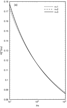
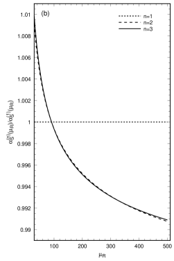
Figure 1: Comparison between the 1st, 2nd and 3rd order running of $\mbox{$\alpha_{S}$}(\mu_{R})$ for $\mbox{$\alpha_{S}$}(M_{Z})=0.118$. Fig. 1a shows $\mbox{$\alpha_{S}$}^{(n)}(\mu_{R})$ from 10 GeV to 1000 GeV while Fig. 1b gives the relative change with respect to the 1st order running over the relevant energy range from 30 GeV to 500 GeV.

In order to calculate an observable

${\cal O}^{data}$ within perturbative QCD we have to introduce the renormalization scale $\mu_{R}$.

However, no matter what scale we choose, it cannot affect the prediction for the physical observable. This statement can be formalized in the

renormalization group equation for the running coupling constant $\mbox{$\alpha_{S}$}(\mu_{R})$. Both the coupling constant and the matrix element coefficients

depend on the renormalization scale while the physical quantity does not. This means that

when measuring $\alpha_{S}$ we have to specify the

renormalization scale so that the extracted $\alpha_{S}$ will be the value of $\alpha_{S}$ at that particular renormalization scale. Of course, all possible choices of the renormalization scale are related to each other by virtue of the renormalization group equation. Relative to a fixed scale, $M_{Z}$, the $n$-loop running coupling constant at scale $\mu_{R}=\lambda M_{Z}$ is given by,

$$\mbox{$\alpha_{S}$}(\mu_{R})=\frac{\mbox{$\alpha_{S}$}(M_{Z})}{1+\mbox{$\alpha_{S}$}(M_{Z})L^{(n)}(\lambda)}$$ (1)

where,

$$L^{(1)}(\lambda) = b_{0}\log\left(\lambda\right),$$ (2)

$$L^{(2)}(\lambda) = (b_{0}+b_{1}\mbox{$\alpha_{S}$}(M_{Z}))\log\left(\lambda\right),$$ (3)

$$L^{(3)}(\lambda) = (b_{0}+b_{1}\mbox{$\alpha_{S}$}(M_{Z})+b_{2}^{\overline{\mbox{\tiny MS}}}\mbox{$\alpha_{S}$}^{2}(M_{Z}))\log\left(\lambda\right)-\frac{b_{0}b_{1}}{2}\mbox{$\alpha_{S}$}^{2}(M_{Z})\log^{2}\left(\lambda\right).$$ (4)

The first three coefficients of the Callan-Symanzik $\beta$-function are given by [19, 20, 21],

$$b_{0} = \frac{11N_{c}-2n_{f}}{6\pi},$$

$$b_{1} = \frac{34N_{c}^{2}-13N_{c}n_{f}+3n_{f}/N_{c}}{24\pi^{2}},$$ (5)

$$b_{2}^{\overline{\mbox{\tiny MS}}} = \frac{5714N_{c}^{3}-3391N_{c}^{2}n_{f}+224N_{c}n_{f}^{2}+507n_{f}+54n_{f}/N_{c}^{2}-66n_{f}^{2}/N_{c}}{3456\pi^{3}},$$

where $N_{c}$ is the number of colors and $n_{f}$ the

number of active flavors. Note that while $b_{0}$ and $b_{1}$ are independent

of the renormalization scheme, $b_{2}$ is renormalization scheme dependent. The expression given here is for the $\overline{\mbox{MS}}$ scheme which we use throughout the paper.

For the processes we will consider, the momentum transfer

ranges from 30 GeV up to around 500 GeV.

In Fig. 1a we show the running $\alpha_{S}$ in this range for

$\mbox{$\alpha_{S}$}(M_{Z})=0.118$. We see that the differences between the evolution at different orders is rather small in the relevant energy range, essentially because $\mbox{$\alpha_{S}$}(M_{Z})$ and $\log(\lambda)$ are both small. To see the differences more clearly,

Fig. 1b shows the relative change in $\mbox{$\alpha_{S}$}(\mu_{R})$

with respect to the 1st order evolution.

The percentage change between 1st and 2nd order evolution in the range from 30 GeV to 500 GeV is less than $\pm$1% and could be safely ignored with the present level of theoretical

and experimental accuracy. In addition, the difference

between 2nd and 3rd order is completely negligible. Therefore, in the rest of the paper we will use the 2-loop evolution as given in

eq. 3.

2.2 Extracting $\alpha_{S}$

Measuring $\alpha_{S}$ from an observable ${\cal O}^{data}$ is, in principle,

rather straightforward provided higher twist effects and other non-perturbative effects are small so that the perturbative expansion can be considered a reliable estimate of the cross section. In other words, we calculate the perturbative expansion ${\cal O}^{pert}$ and equate it with the data,

$${\cal O}^{data}\equiv{\cal O}^{pert}.$$ (6)

For example, for the single jet inclusive transverse energy distribution,

$${\cal O}=\frac{d\sigma}{dE_{T}},$$

there is a good agreement between perturbative calculations and the data over 7 orders of magnitude in the cross section

in the range $30\leq E_{T}\leq 500$ GeV [22, 23].

By comparing data with theory for each $E_{T}$-bin, we make many independent measurements of

$\alpha_{S}$ at a specified

renormalization scale assuming no correlated bin-to-bin

experimental systematic errors.

The perturbative expansion can be written,

$${\cal O}^{pert}=\mbox{$\alpha_{S}$}^{m}(\mu_{R})\hat{\cal O}^{(0)}K^{(\infty)}(\mbox{$\alpha_{S}$}(\mu_{R}),\mu_{R}/Q_{R}),$$ (7)

where the scale $Q_{R}$ is the characteristic scale for the observable under

consideration which will be the transverse

energy of the jet for the single jet inclusive transverse energy distribution. The Born-prediction is given by $\mbox{$\alpha_{S}$}^{m}(\mu_{R})\hat{\cal O}^{(0)}$ and all the higher order corrections are contained in the $K$-factor,

$$K^{(n)}(\mbox{$\alpha_{S}$}(\mu_{R}),\mu_{R}/Q_{R})=1+\sum_{l=1}^{n}\mbox{$\alpha_{S}$}^{l}(\mu_{R})k_{l}(\mu_{R}/Q_{R}).$$ (8)

For the single jet inclusive transverse energy distribution,

$m=2$ and the $K$-factor is currently

known up to next-to-leading order, giving $K^{(1)}$.

Once the $K$-factor has been calculated up to the $n$-th order in $\alpha_{S}$, the first step in extracting the $n$-th order $\mbox{$\alpha_{S}$}^{(n)}$

is to determine the leading order $\mbox{$\alpha_{S}$}^{(0)}$ together with its experimental uncertainties.

This is simply given by the ratio of the data over the leading order coefficient $\hat{\cal O}^{(0)}$

$${\mbox{$\alpha_{S}$}^{(0)}}=\sqrt[m]{\frac{{\cal O}^{data}}{\hat{\cal O}^{(0)}}},$$ (9)

and does not depend on the renormalization

scale.

While the determination of the leading order $\alpha_{S}$

has no useful theoretical interpretation it is nevertheless a very convenient

manner in which to parametrize the data.

In principle, all we need from an experiment is the leading order $\alpha_{S}$ as given in eq. 9 together with the experimental errors. From here

we can determine $\mbox{$\alpha_{S}$}^{(n)}$ values without referring back to the original data. For example, given $K^{(n)}$, the $n$-th order $\alpha_{S}$ is given by,

$${\mbox{$\alpha_{S}$}^{(n)}}(\mu_{R})=\frac{\mbox{$\alpha_{S}$}^{(0)}}{\sqrt[m]{K^{(n)}(\mbox{$\alpha_{S}$}^{(n)}(\mu_{R}),\mu_{R}/Q_{R})}},$$ (10)

so that $\mbox{$\alpha_{S}$}^{(n)}(\mu_{R})$ are just the roots of the $(m+n)$-th order polynomial,

$$[{\mbox{$\alpha_{S}$}^{(n)}}(\mu_{R})]^{m}\left(1+\sum_{l=1}^{n}[\mbox{$\alpha_{S}$}^{(n)}(\mu_{R})]^{l}k_{l}(\mu_{R}/Q_{R})\right)-[\mbox{$\alpha_{S}$}^{(0)}]^{m}=0.$$ (11)

2.3 Theoretical Uncertainty

For the processes of interest, only the first order corrections

are currently known. Therefore, we use the leading order $\mbox{$\alpha_{S}$}^{(0)}$ (with experimental errors)

and solve the $(m+1)$th order polynomial,

$$k_{1}(\mu_{R}/Q_{R})[\mbox{$\alpha_{S}$}^{(1)}(\mu_{R})]^{(m+1)}+[\mbox{$\alpha_{S}$}^{(1)}(\mu_{R})]^{m}-[\mbox{$\alpha_{S}$}^{(0)}]^{m}=0,$$ (12)

with $\mu_{R}=\mu_{0}$ to find $\mbox{$\alpha_{S}$}^{(1)}(\mu_{0})$. For the single jet inclusive transverse energy distribution,

we choose $\mu_{0}=Q_{R}=E_{T}$.

To estimate the theoretical uncertainty we can extract $\alpha_{S}$ at renormalization scale $\mu_{R}=\lambda\mu_{0}$ which we subsequently evolve back to scale $\mu_{0}$ using the 2-loop renormalization group running of $\alpha_{S}$. Quantitatively this means we solve eq. 12 with

$\mu_{R}=\lambda\mu_{0}$ and determine,

$$\mbox{$\alpha_{S}$}(\mu_{0};\mu_{R}=\lambda\mu_{0})=\frac{\mbox{$\alpha_{S}$}(\lambda\mu_{0})}{1+\mbox{$\alpha_{S}$}(\lambda\mu_{0})L^{(2)}(1/\lambda)}.$$ (13)

By defining,

$$\frac{\Delta\mbox{$\alpha_{S}$}(\lambda)}{\mbox{$\alpha_{S}$}}\equiv\frac{\mbox{$\alpha_{S}$}(\mu_{0};\mu_{R}=\lambda\mu_{0})-\mbox{$\alpha_{S}$}(\mu_{0};\mu_{R}=\mu_{0})}{\mbox{$\alpha_{S}$}(\mu_{0};\mu_{R}=\mu_{0})},$$ (14)

we can estimate the theoretical uncertainty in $\alpha_{S}$.

The reason $\Delta\mbox{$\alpha_{S}$}$ is non-zero is due to the fact that the NLO coefficient $k_{1}(\mu_{R}=\lambda\mu_{0})$ is only the first order correction and rest of the higher order corrections are neglected. The behavior of $k_{1}$ under renormalization scale changes is,

$$k_{1}(\mu_{R}=\lambda\mu_{0})=k_{1}(\mu_{R}=\mu_{0})+mb_{0}\log(\lambda)\ .$$ (15)

This shift changes the solution of eq. 12 giving us

$\mbox{$\alpha_{S}$}(\lambda\mu_{0})$. However, evolving back to $\mu_{R}=\mu_{0}$ using

eq. 13 does not exactly

match the change due to eq. 15. In fact the shift in $\alpha_{S}$ due to this mismatch

has a relatively simple form for small $\log(\lambda)$,

$$\frac{\Delta\mbox{$\alpha_{S}$}(\lambda)}{\mbox{$\alpha_{S}$}}\sim\mbox{$\alpha_{S}$}^{2}\left(\frac{(m+1)b_{0}k_{1}(\mu_{R}=\mu_{0})}{m+(m+1)\mbox{$\alpha_{S}$}k_{1}(\mu_{R}=\mu_{0})}+b_{1}\right)\log(\lambda)+{\cal O}(\log^{2}(\lambda)).$$ (16)

To extract the central value of $\mbox{$\alpha_{S}$}(\mu_{0})$ and its theoretical uncertainty we can follow many different procedures. We will outline two of them here.

Method I

The first procedure is rather straightforward. We take $\mu_{R}=\mu_{0}$ as the central scale and vary the renormalization scale between $\mu_{R}=\mu_{0}/2$ and $\mu_{R}=2\mu_{0}$ to estimate the uncertainty. Explicitly this means,

$$\mbox{$\alpha_{S}$}^{(1)}(\mu_{0}) = \frac{1}{2}\Big{(}\mbox{$\alpha_{S}$}(\mu_{0};\mu_{R}=2\mu_{0})+\mbox{$\alpha_{S}$}(\mu_{0};\mu_{R}=\mu_{0}/2)\Big{)},$$

$$\Delta\mbox{$\alpha_{S}$}^{(1)}(\mu_{0}) = \frac{1}{2}\Big{(}\mbox{$\alpha_{S}$}(\mu_{0};\mu_{R}=2\mu_{0})-\mbox{$\alpha_{S}$}(\mu_{0};\mu_{R}=\mu_{0}/2)\Big{)}.$$ (17)

Method II

The second procedure is based on the fact that $\Delta\mbox{$\alpha_{S}$}/\mbox{$\alpha_{S}$}$ has a minimum. This occurs when $\lambda=\lambda_{0}=\exp(-k_{1}(\mu_{R}=\mu_{0})/mb_{0})$

so that the first order correction vanishes, $k_{1}(\mu_{R}=\lambda_{0}\mu_{0})=0$ and $\mbox{$\alpha_{S}$}^{(0)}=\mbox{$\alpha_{S}$}^{(1)}(\mu_{R}=\lambda_{0}\mu_{0})$.

Now we can define $\mbox{$\alpha_{S}$}^{(1)}(\mu_{0})$ and the theoretical uncertainty in the following manner,

$$\mbox{$\alpha_{S}$}^{(1)}(\mu_{0}) = \frac{1}{2}\Big{(}\mbox{$\alpha_{S}$}(\mu_{0};\mu_{R}=\mu_{0})+\mbox{$\alpha_{S}$}(\mu_{0};\mu_{R}=\lambda_{0}\mu_{0})\Big{)},$$

$$\Delta\mbox{$\alpha_{S}$}^{(1)}(\mu_{0}) = \frac{1}{2}\Big{(}\mbox{$\alpha_{S}$}(\mu_{0};\mu_{R}=\mu_{0})-\mbox{$\alpha_{S}$}(\mu_{0};\mu_{R}=\lambda_{0}\mu_{0})\Big{)}.$$ (18)

There are two major differences between the two methods of

estimating the theoretical uncertainty. First, the estimated theoretical uncertainty is generally larger in method I than in method II and second, the central value of $\mbox{$\alpha_{S}$}(\mu_{0})$ using method II is slightly lower, but by construction it lies within the range of uncertainty of method I.

3 The one-jet inclusive transverse energy distribution

The one-jet inclusive transverse energy distribution ($d\sigma/dE_{T}$) has a straightforward interpretation: the transverse energy of the leading jet ($E_{T}$) is directly related to the impact parameter $b_{impact}$ (or the distance scale) in the underlying hard parton-parton scattering by the relation

$$\left(\frac{b_{impact}}{1\ {\rm fm}}\right)=0.0507\times\left(\frac{E_{T}}{100\ {\rm GeV}}\right)^{-1}.$$ (19)

Therefore by studying this particular distribution we probe rather directly the physics over a wide range of distance scales within one single measurement. For the published CDF data, the transverse energies range from 30 GeV up to 500 GeV. In other words, we probe the dynamics of the parton-parton scattering from a distance scale of 0.169 fm all the way down to 0.01 fm. The obvious quantity to study is therefore $\alpha_{S}$ extracted at renormalization scale $\mu_{R}=E_{T}$. Subsequently we can test QCD

by comparing the measured $\alpha_{S}$ at the different distance scales with the running $\alpha_{S}$ predicted by QCD. The comparison will be sensitive to new physics, the most

obvious being substructure of the quarks. However,

deviations from QCD at small distance scales will also show up as violations of the running of $\alpha_{S}$. To perform the comparison with QCD we will use two methods, each of which has its own interest. The first one assumes the evolution is correctly

given by QCD to extract $\alpha_{S}$ at a common scale, $\mu_{R}=M_{Z}$, while the second method quantifies deviations from purely QCD-like evolution.

3.1 The QCD-fit

In the first method we assume the correctness of QCD to describe the parton-parton scattering at all distance scales relevant in this measurement. This enables us to extract the best possible value of $\mbox{$\alpha_{S}$}(M_{Z})$ using a given data set. Each $E_{T}$-bin in the differential cross section gives an independent measurement of $\mbox{$\alpha_{S}$}(E_{T})$ which we subsequently can evolve to $\mbox{$\alpha_{S}$}(M_{Z})$ using the renormalization group equation. The published CDF data set has 38 individual $E_{T}$-bins, and therefore yields 38 independent measurements of $\mbox{$\alpha_{S}$}(M_{Z})$, so that the statistical error will be negligible compared to the common systematic error which has two components. The first is the calorimeter response correction together with fragmentation/hadronization effects and

the second is the luminosity uncertainty.

The luminosity uncertainty can be reduced

using the $W$-boson production cross section ($\sigma_{W}$) as a luminosity measurement. Experimentally this simply involves counting the number of $W$-boson events and normalizing $d\sigma/dE_{T}$

respectively, i.e. we study $1/\sigma_{W}d\sigma/dE_{T}$ so that the luminosity uncertainty cancels. Theoretically, $\sigma_{W}$ is the best known cross section at hadron colliders, known up to 2-loop QCD corrections [24].

Therefore

$1/\sigma_{W}d\sigma/dE_{T}$ can be calculated

consistently order by order in perturbative QCD and compared to experiment to extract $\alpha_{S}$.

This method of normalizing the cross section

can easily be generalized to all observables.

3.2 The Best-fit

It may turn out that the measured $\mbox{$\alpha_{S}$}(M_{Z})$ is not independent

of the $E_{T}$ values it was extracted from. This indicates either deficiencies in the input PDF or, more interestingly, deviations from the underlying QCD theory. Parametrizing possible deviations from the QCD condition $\partial\mbox{$\alpha_{S}$}(M_{Z};\mu_{R}=E_{T})/\partial E_{T}=0$ will give us an excellent check on the theory. We therefore quantify deviations from QCD by allowing

$\partial\mbox{$\alpha_{S}$}(M_{Z};\mu_{R}=E_{T})/\partial E_{T}=f(E_{T})\neq 0$.

The size of the deviation $f(E_{T})$ and its uncertainty will tell us how well the data set fits QCD. More interestingly, by evolving the fit to $\mbox{$\alpha_{S}$}(M_{Z};\mu_{R}=E_{T})$ back to $\mbox{$\alpha_{S}$}(E_{T})$ we obtain

the “Best-fit” prediction for the evolution of $\alpha_{S}$. By extrapolating the fit to larger and smaller scales we find the permissible range of evolution for $\mbox{$\alpha_{S}$}(\mu_{R})$ allowing for small deviations from QCD in the current data set.

We can then compare with $\alpha_{S}$ measurements at different energy scales and see how compatible the deviations are with the other measurements, in particular the slower running that may be suggested by the low energy data [25]. While the systematic error dominates in the “QCD-fit” method, here the systematic error (including the theoretical uncertainty) will merely affect the overall normalization of the $\alpha_{S}$ evolution and not the shape.

In fact by normalizing the curve to the world average value of $\mbox{$\alpha_{S}$}(M_{Z})$ we can completely remove the systematic error.

4 The CDF data

The CDF data used in this analysis is from the ’88-’89 TEVATRON collider run at Fermilab which yielded an integrated luminosity of 4.2 pb^-1. The data was taken from the preprint version [26] of the published letter [23]. The preprint tabulates the results together with the separated statistical and systematic errors. Unfortunately the error-analysis in the current paper is limited by the fact that the published results do not have the necessary detailed discussion of the systematic errors needed for a more rigorous error treatment. We will use an ad-hoc procedure to separate a common systematic error and a bin-by-bin statistical error. Also the removal of the luminosity error using the $W$-boson cross section cannot be applied, as this would require a careful simultaneous study of the $W$-boson and jet data. However, both the CDF and DØ collaborations can incorporate a proper error analysis and removal of the luminosity error using the new run 1A/B data sets.

Our purpose here is to illustrate the methods rather than

produce a definitive measurement and error analysis.

The one-jet inclusive transverse energy

distribution of CDF is constructed by including all the jets, which are defined according to the

Snowmass algorithm with a conesize of 0.7 [27], in the pseudo-rapidity range between 0.1 and 0.7. This means

that this particular distribution is not exactly the transverse energy distribution of the leading jet as would be preferred for the $\alpha_{S}$ measurement, but contains some

softer jets. However, although small deviations from the leading jet $E_{T}$ distribution can be expected at small $E_{T}$, for high-$E_{T}$ bins there is virtually no difference between the two distributions.

Some of the features of the particular data taking for the ’88-’89 run will be reflected in the $\alpha_{S}$ measurement. First of all, the statistical error is affected by the different event triggers, each with its own

prescaling factor. The off-line $E_{T}$ cuts (ensuring 98% efficiency in the data taking) for the three triggers are 35 GeV (with prescaling factor

1 per 300 events), 60 GeV (1 per 30 events) and 100 GeV (not prescaled) [23]. This means the statistical errors fall into three distinct regions which eventually will be reflected in the statistical error on $\alpha_{S}$.

Second, the systematic error is due to the luminosity measurement and the detector response combined with the hadron distribution within the jets (which is modelled by

fragmentation/hadronization Monte Carlo’s). The systematic error quoted contains all these uncertainties and most of the error will be common to all the bins. Apart from the luminosity error,

the systematic error falls into two separate regions.

Below $E_{T}=80$ GeV, the systematic error is large, decreasing from as high as $\pm$60% at 35 GeV to $\pm$22% at 80 GeV. As a result, the $\alpha_{S}$ measurement below 80 GeV is strongly affected by short range correlated systematic errors.

For $E_{T}>80$ GeV, however, the systematic error is fairly constant with a typical value of $\pm$22%, making the short range systematic error correlations small. Again these characteristics of the data will eventually be reflected in the measured $\alpha_{S}$.

5 Determining $\alpha_{S}$

To extract $\alpha_{S}$ we use the next-to-leading order parton level Monte Carlo JETRAD [28] which is based on the techniques described in refs. [29, 30] and the matrix elements of ref. [31].

The cuts and jet algorithm applied directly to the partons, were modelled as closely as possible to the experimental set-up. Using the Monte Carlo we calculated the Born coefficient

${\hat{O}}^{(0)}$ and the next-to-leading order coefficient $k^{(1)}$ as defined in eqs. 7 and 8 for the MRSA^′ PDF set of ref. [6].

These distribution functions use the low-$x$ $F_{2}$ data from the 1993 data taking run at HERA. However, we are mainly concerned with $x$ values typically greater

than few $\times 10^{-2}$, and there is little impact from HERA

data in this range. To see this, we also consider the older MRSD0^′

and MRSD-^′ parameterisations [3]. Using eq. 9 we determine the leading order $\mbox{$\alpha_{S}$}^{(0)}$ from the

CDF data including the statistical and systematic errors. The results are listed in Table 1 together with the next-to-leading order coefficients determined at a renormalization/factorization scale equal to the $E_{T}$ value of the bin and the Monte Carlo integration error.

This table contains all the information needed to extract the

next-to-leading order $\alpha_{S}$.

5.1 Measurement of $\mbox{$\alpha_{S}$}^{(1)}(E_{T})$

$E_{T}$	MRSA′
(GeV)	$\mbox{$\alpha_{S}$}^{(0)}$	$k_{1}$	$\mbox{$\alpha_{S}$}^{(1)}(E_{T})$	$\mbox{$\alpha_{S}$}^{(1)}(M_{Z})\pm 0.008$
35.48	${0.163\pm 0.003}^{+.027}_{-.049}$	$2.90\pm 0.24$	$0.138\pm 0.028\pm 0.007$	$0.118\pm 0.013\pm 0.005$
41.63	${0.154\pm 0.001}^{+.025}_{-.044}$	$2.94\pm 0.26$	$0.131\pm 0.026\pm 0.006$	$0.116\pm 0.013\pm 0.005$
47.61	${0.149\pm 0.001}^{+.024}_{-.039}$	$3.18\pm 0.29$	$0.126\pm 0.023\pm 0.006$	$0.114\pm 0.011\pm 0.005$
53.54	${0.149\pm 0.002}^{+.022}_{-.033}$	$3.42\pm 0.27$	$0.125\pm 0.020\pm 0.006$	$0.115\pm 0.009\pm 0.005$
59.93	${0.143\pm 0.003}^{+.021}_{-.029}$	$3.04\pm 0.24$	$0.122\pm 0.019\pm 0.005$	$0.115\pm 0.009\pm 0.004$
66.23	${0.144\pm 0.003}^{+.019}_{-.024}$	$3.34\pm 0.23$	$0.122\pm 0.016\pm 0.005$	$0.116\pm 0.007\pm 0.005$
72.29	${0.145\pm 0.001}^{+.019}_{-.021}$	$2.80\pm 0.25$	$0.125\pm 0.015\pm 0.005$	$0.121\pm 0.006\pm 0.005$
78.15	${0.147\pm 0.002}^{+.018}_{-.018}$	$3.11\pm 0.24$	$0.125\pm 0.013\pm 0.005$	$0.122\pm 0.005\pm 0.005$
83.81	${0.153\pm 0.002}^{+.018}_{-.016}$	$3.57\pm 0.21$	$0.127\pm 0.012\pm 0.006$	$0.125\pm 0.004\pm 0.006$
89.31	${0.148\pm 0.002}^{+.018}_{-.016}$	$3.35\pm 0.25$	$0.125\pm 0.013\pm 0.006$	$0.124\pm 0.005\pm 0.006$
94.82	${0.147\pm 0.003}^{+.018}_{-.016}$	$3.39\pm 0.22$	$0.123\pm 0.013\pm 0.006$	$0.124\pm 0.005\pm 0.006$
100.19	${0.145\pm 0.003}^{+.018}_{-.016}$	$3.73\pm 0.23$	$0.120\pm 0.012\pm 0.005$	$0.122\pm 0.005\pm 0.006$
105.60	${0.144\pm 0.004}^{+.017}_{-.016}$	$3.45\pm 0.23$	$0.121\pm 0.012\pm 0.005$	$0.124\pm 0.005\pm 0.006$
111.04	${0.143\pm 0.004}^{+.017}_{-.015}$	$3.28\pm 0.23$	$0.121\pm 0.012\pm 0.005$	$0.125\pm 0.005\pm 0.006$
116.44	${0.135\pm 0.001}^{+.017}_{-.016}$	$3.77\pm 0.22$	$0.113\pm 0.012\pm 0.005$	$0.118\pm 0.005\pm 0.005$
121.76	${0.136\pm 0.001}^{+.017}_{-.016}$	$3.52\pm 0.22$	$0.115\pm 0.012\pm 0.005$	$0.120\pm 0.005\pm 0.005$
127.12	${0.135\pm 0.001}^{+.017}_{-.016}$	$3.50\pm 0.21$	$0.114\pm 0.012\pm 0.005$	$0.120\pm 0.006\pm 0.005$
132.49	${0.134\pm 0.001}^{+.017}_{-.016}$	$3.77\pm 0.23$	$0.113\pm 0.012\pm 0.005$	$0.119\pm 0.005\pm 0.005$
137.77	${0.135\pm 0.002}^{+.017}_{-.016}$	$3.44\pm 0.20$	$0.114\pm 0.012\pm 0.005$	$0.121\pm 0.006\pm 0.005$
143.05	${0.134\pm 0.002}^{+.017}_{-.016}$	$3.77\pm 0.22$	$0.112\pm 0.012\pm 0.005$	$0.120\pm 0.006\pm 0.005$
148.48	${0.134\pm 0.002}^{+.016}_{-.015}$	$4.10\pm 0.22$	$0.111\pm 0.011\pm 0.005$	$0.119\pm 0.005\pm 0.005$
153.71	${0.132\pm 0.002}^{+.016}_{-.015}$	$3.78\pm 0.22$	$0.111\pm 0.012\pm 0.004$	$0.120\pm 0.006\pm 0.005$
158.93	${0.133\pm 0.003}^{+.016}_{-.015}$	$3.54\pm 0.20$	$0.112\pm 0.011\pm 0.004$	$0.122\pm 0.006\pm 0.005$
164.25	${0.133\pm 0.003}^{+.016}_{-.015}$	$4.26\pm 0.19$	$0.110\pm 0.011\pm 0.005$	$0.119\pm 0.005\pm 0.006$
171.89	${0.135\pm 0.003}^{+.016}_{-.015}$	$3.95\pm 0.16$	$0.113\pm 0.011\pm 0.005$	$0.124\pm 0.005\pm 0.006$
182.20	${0.135\pm 0.003}^{+.015}_{-.014}$	$3.98\pm 0.14$	$0.112\pm 0.011\pm 0.005$	$0.125\pm 0.005\pm 0.006$
193.04	${0.128\pm 0.004}^{+.016}_{-.015}$	$4.05\pm 0.14$	$0.107\pm 0.011\pm 0.004$	$0.119\pm 0.006\pm 0.005$
203.47	${0.116\pm 0.005}^{+.017}_{-.016}$	$3.75\pm 0.14$	$0.099\pm 0.013\pm 0.003$	$0.111\pm 0.008\pm 0.004$
215.73	${0.120\pm 0.005}^{+.016}_{-.015}$	$4.15\pm 0.12$	$0.101\pm 0.012\pm 0.004$	$0.113\pm 0.007\pm 0.005$
231.88	${0.122\pm 0.006}^{+.015}_{-.014}$	$4.22\pm 0.11$	$0.102\pm 0.011\pm 0.004$	$0.116\pm 0.007\pm 0.005$
246.86	${0.121\pm 0.008}^{+.016}_{-.015}$	$4.32\pm 0.11$	$0.101\pm 0.012\pm 0.004$	$0.116\pm 0.008\pm 0.005$
264.86	${0.115\pm 0.011}^{+.016}_{-.015}$	$4.17\pm 0.10$	$0.097\pm 0.014\pm 0.003$	$0.112\pm 0.010\pm 0.004$
281.96	${0.140\pm 0.013}^{+.014}_{-.013}$	$4.31\pm 0.10$	$0.114\pm 0.013\pm 0.005$	$0.137\pm 0.011\pm 0.008$
302.22	${0.137\pm 0.022}^{+.014}_{-.013}$	$4.28\pm 0.09$	$0.112\pm 0.019\pm 0.005$	$0.136\pm 0.019\pm 0.007$
322.87	${0.124\pm 0.035}^{+.016}_{-.015}$	$4.60\pm 0.09$	$0.103\pm 0.028\pm 0.004$	$0.123\pm 0.032\pm 0.006$
343.88	${0.154\pm 0.056}^{+.016}_{-.014}$	$4.55\pm 0.08$	$0.123\pm 0.041\pm 0.006$	$0.155\pm 0.056\pm 0.010$
380.72	${0.161\pm 0.101}^{+.016}_{-.014}$	$4.66\pm 0.07$	$0.127\pm 0.078\pm 0.007$	$0.166\pm 0.109\pm 0.012$
418.55	${0.188\pm 0.143}^{+.018}_{-.017}$	$4.86\pm 0.07$	$0.144\pm 0.224\pm 0.010$	$0.201\pm 0.251\pm 0.020$

Table 1: The extracted leading order $\mbox{$\alpha_{S}$}^{(0)}$ with statistical and systematical errors based on the published CDF data [23]. The higher order coefficient $k_{1}$ for $\mu_{R}=\mu_{F}=E_{T}$ is also shown with its associated MC-integration error. The last two columns give $\mbox{$\alpha_{S}$}^{(1)}$ based on the solution of eq. 12 with the combined statistical/systematic errors from [23] and the theoretical uncertainty estimate using method I as described in the text.

Figure 2: The uncertainty in $\mbox{$\alpha_{S}$}(E_{T})$ due to variation in the renormalization scale (solid line). Also shown is the logarithmic tangent of eq. 16 (dashed line) which has a simple analytic form.

Finally we are in a position to determine the next-to-leading order $\mbox{$\alpha_{S}$}^{(1)}$ and the associated theoretical uncertainty. We combine the experimental statistical and systematic errors on the leading order $\mbox{$\alpha_{S}$}^{(0)}$ in quadrature and solve eq. 12 with $m=2$ and $\mu_{0}=E_{T}$ to extract $\mbox{$\alpha_{S}$}^{(1)}(E_{T})$.

In fig. 2 we show both the exact $\Delta\mbox{$\alpha_{S}$}(\lambda)/\mbox{$\alpha_{S}$}$ defined by

eq. 14 and its logarithmic tangent as given by eq. 16 for one $E_{T}$-bin. We see that for $0.5<\lambda<2$, the linear approximation is reasonable. The extracted values of $\mbox{$\alpha_{S}$}^{(1)}(E_{T})$

(with the associated theoretical errors)

defined by eqs. 2.3 and 2.3

for the 38 transverse energy bins are given in Table 1. Numerically, the major difference between the two methods of estimating the theoretical uncertainty is that in method I the estimated theoretical uncertainty is of the order of 4%, while method II gives a smaller theoretical uncertainty of typically 2%.

The central value of $\mbox{$\alpha_{S}$}^{(1)}(E_{T})$ using method II is lower by 2%, but remains within the uncertainty of method I. For the rest of the paper we will use the

$\mbox{$\alpha_{S}$}(E_{T})$ extraction based on method I.

As a rough guide, changing to method II means

reducing the theoretical uncertainty and lowering the central value by 2%.

5.2 Measurement of $\mbox{$\alpha_{S}$}^{(1)}(M_{Z})$

The next step is to determine the strong coupling constant at $M_{Z}$ by evolving from $\mu_{R}=E_{T}$ to $\mu_{R}=M_{Z}$

using the 2-loop evolution equation eq. 3. To extract the common long range systematic error,

$\Delta\mbox{$\alpha_{S}$}^{sys}$, we employed the following ad hoc procedure.

Because $\mbox{$\alpha_{S}$}(M_{Z};\mu_{R}=E_{T})$ is supposed to be independent of $E_{T}$ we can define $\Delta\mbox{$\alpha_{S}$}^{sys}$ such that,

$$\chi^{2}=\frac{1}{N_{bins}}\sum_{i=1}^{N_{bins}}\frac{\left[\mbox{$\alpha_{S}$}^{(1)}(M_{Z};\mu_{R}=E_{T}^{(i)})-<\mbox{$\alpha_{S}$}(M_{Z})>\right]^{2}}{\left[\Delta\mbox{$\alpha_{S}$}^{exp}(M_{Z};\mu_{R}=E_{T}^{(i)})-\Delta\mbox{$\alpha_{S}$}^{sys}\right]^{2}}=1.$$ (20)

Here $E_{T}^{(i)}$ refers to the specific bin-values. This procedure gives us a value for $\Delta\mbox{$\alpha_{S}$}^{sys}=0.008$, which

is then common to all values of $\alpha_{S}$. The remaining errors,

$\Delta\mbox{$\alpha_{S}$}^{stat}=\Delta\mbox{$\alpha_{S}$}^{exp}-\Delta\mbox{$\alpha_{S}$}^{sys}$, are a combination of statistical errors and shorter range correlated systematic errors. Fig. 3 and Table 1 display the values of $\mbox{$\alpha_{S}$}(M_{Z})$ extracted from the 38 $E_{T}$ bins with the associated

experimental statistical error and the estimate of the theoretical uncertainty. The systematic error is an overall factor of $\pm 0.008$. We see that measured value of $\mbox{$\alpha_{S}$}(M_{Z})$ is essentially independent of $E_{T}$ for the MRSA^′ parton density functions. This is also true of the MRSD0^′ and MRSD-^′ parameterisations.

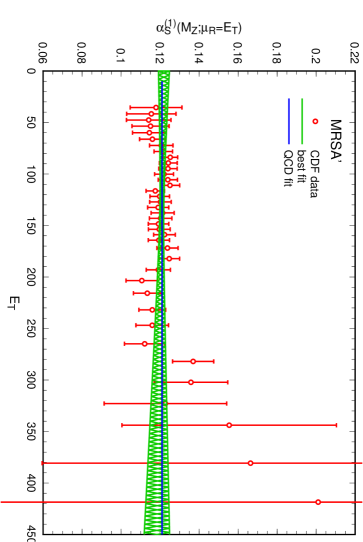
Figure 3: The extracted $\mbox{$\alpha_{S}$}^{(1)}(M_{Z},\mu_{R}=E_{T})$ as a function of $E_{T}$ for the MRSA^′ parameterisation. The QCD-fit yields $\mbox{$\alpha_{S}$}^{(1)}(M_{Z})=0.121\pm 0.001\pm 0.008\pm 0.005$. The 68% confidence level Best-fits are shown as shaded bands.

5.3 The QCD-fit to $\mbox{$\alpha_{S}$}^{(1)}(M_{Z})$

To compare the obtained result with QCD we first assume that next-to-leading order QCD is sufficient to describe the data. In this case

$\partial\mbox{$\alpha_{S}$}(M_{Z};\mu_{R}=E_{T})/\partial E_{T}=0$ and we can

perform an error weighted average to obtain the average $\mbox{$\alpha_{S}$}^{(1)}(M_{Z})$,

$$\mbox{$\alpha_{S}$}^{(1)}(M_{Z})=\frac{1}{w}\sum_{i=1}^{N_{bins}}w_{i}\mbox{$\alpha_{S}$}^{(1)}(M_{Z};\mu_{R}=E_{T}^{(i)}),$$ (21)

where,

$$\frac{1}{w_{i}} = \Delta\mbox{$\alpha_{S}$}^{stat}(M_{Z};\mu_{R}=E_{T}^{(i)}),$$

$$w = \sum_{i=1}^{N_{bins}}w_{i}.$$ (22)

The resulting values for $\mbox{$\alpha_{S}$}^{(1)}(M_{Z})$ are,

$$\mbox{$\alpha_{S}$}^{(1)}(M_{Z}) = 0.119\pm 0.001\pm 0.008\pm 0.005\ \mbox{for MRSD0${}^{\prime}$}$$

$$\mbox{$\alpha_{S}$}^{(1)}(M_{Z}) = 0.121\pm 0.001\pm 0.008\pm 0.005\ \mbox{for MRSA${}^{\prime}$}$$ (23)

$$\mbox{$\alpha_{S}$}^{(1)}(M_{Z}) = 0.124\pm 0.001\pm 0.008\pm 0.005\ \mbox{for MRSD-${}^{\prime}$}$$

where the first error is the statistical error, the second error the systematic error and the third error the theoretical uncertainty estimate based on method I. We see that the error from using different PDF as input is approximately $\pm 0.002$.

A note of caution is in order. In the analysis presented here, we have taken PDF’s which have a $Q^{2}$ evolution based on $\mbox{$\alpha_{S}$}^{DIS}(M_{Z})=0.113\pm 0.005$ [6], while the explicit $\alpha_{S}$ in the matrix elements was varied. This can only be consistent if the extracted value of $\mbox{$\alpha_{S}$}(M_{Z})$ is in agreement with $\mbox{$\alpha_{S}$}^{DIS}(M_{Z})$. However, we see that this is indeed the case (c.f. 5.3) once the

statistical, systematic and theoretical errors are combined. With the new high statistic data sets of run 1A/B, the statistical and systematic errors

will be significantly reduced and it will be necessary to utilise PDF’s with $Q^{2}$ evolution for a variety of $\mbox{$\alpha_{S}$}(M_{Z})$ values. Recently such PDF sets have come available [32, 33] so that a more consistent determination of $\alpha_{S}$ will be possible

once the new data becomes available.

5.4 The Best-fit to $\mbox{$\alpha_{S}$}^{(1)}(M_{Z})$

PDF	$a$	$b$	$c$	$d$
MRSD0′	0.119	0.0038	0.0008	11.0
MRSA′	0.120	-0.0010	0.0010	6.8
MRSD-′	0.124	-0.0014	0.0011	6.2

Table 2: Best-fit results from minimum $\chi^{2}$-fit

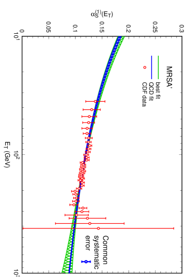
Figure 4: The values of $\mbox{$\alpha_{S}$}^{(1)}(E_{T})$ extracted from the published CDF data as a function of $E_{T}$ together with $\mbox{$\alpha_{S}$}^{(1)}(E_{T})$ from the QCD- and Best-fits evolved from $M_{Z}$ to $E_{T}$ for the MRSA^′ parameterisation.

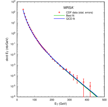
Figure 5: Comparison of the one-jet inclusive transverse energy distribution evaluated using $\mbox{$\alpha_{S}$}^{(1)}(E_{T})$ from the QCD- and Best-fits evolved from $M_{Z}$ to $E_{T}$ for the MRSA^′ parameterisation.

The second comparison with QCD we can perform is a check on the running behavior of $\alpha_{S}$. For such a check, the overall systematic error is not important and the experimental error is reduced considerably. This tests whether $\mbox{$\alpha_{S}$}(M_{Z})$ is independent of the distance scale at which the scattering takes place. To do this we no longer assume $\partial\mbox{$\alpha_{S}$}(M_{Z};\mu_{R}=E_{T})/\partial E_{T}=0$ but allow it to be a constant. If QCD is correct, the constant should be zero within errors.

The results from a minimal $\chi^{2}$ fit to a linear function in $E_{T}$,

$$\mbox{$\alpha_{S}$}^{(1)}(M_{Z};\mu_{R}=E_{T}) = a+b\times\left(\frac{E_{T}}{E_{T}^{0}}-1\right)$$

$$\Delta\mbox{$\alpha_{S}$}^{stat}(M_{Z};\mu_{R}=E_{T}) = c\times\sqrt{1+d\times\left(\frac{E_{T}}{E_{T}^{0}}-1\right)^{2}}\ ,$$ (24)

are given in Table 2 for the MRSD0^′, MRSA^′

and MRSD-^′ parameterisations. The scale $E_{T}^{0}\simeq 130$ GeV gives the minimal one-sigma error. The common systematic error, $\Delta\mbox{$\alpha_{S}$}^{sys}=0.008$

is not affected by the fits. The linear minimal-$\chi^{2}$ fits give a perfect fit to QCD (i.e. no $E_{T}$ dependence) within one sigma over a range from 30 GeV to 500 GeV for MRSA^′ and MRSD-^′,

while the MRSD0^′ results show a small but insignificant dependence on the transverse energy which possibly indicate some problems with the underlying PDF set. It should be stressed that these results are highly non trivial and demonstrate the correctness of QCD over a wide range of momentum transfers (or distance scales) not previously probed.

Although the statistics are rather poor at high $E_{T}$, the new CDF and DØ results should give better results in the region above 200 GeV.

Next we can evolve the Best-fit result from $\mbox{$\alpha_{S}$}(M_{Z};\mu_{R}=E_{T})$ back to $\mbox{$\alpha_{S}$}(E_{T})$ and extrapolate to smaller and larger $E_{T}$ values to obtain the

measured running $\alpha_{S}$ and then compare that with the QCD prediction from the QCD-fit. This comparison is shown in fig. 4 where we can see that the measured evolution agrees perfectly with the QCD evolution for the MRSA^′ parameterisation.

On the other hand, if we use the Best-fit for the MRSD0^′ set,

we find a slower running of the coupling constant

which agrees very well with, in particular, the low energy $\alpha_{S}$ measurements [25].

The results from the new collider run will clarify this and test the running $\alpha_{S}$ behavior much better.

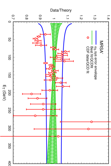
Figure 6: Ratio of the published CDF data and next-to-leading order prediction evaluated using $\mbox{$\alpha_{S}$}^{(1)}(E_{T})$ from the QCD- and Best-fits evolved from $M_{Z}$ to $E_{T}$ for the MRSA^′ parameterisation. The systematic uncertainty is also shown in the QCD-fit based procedure.

Finally, we can use the measured evolution of $\alpha_{S}$ to calculate the one-jet inclusive cross section. The differential distribution is shown in fig. 5, while the more useful data divided by theory result is shown in fig. 6. Both the QCD-fit (including the systematic error) and the Best-fit for the MRSA^′ parameterisation describe the data well. The prescaling thresholds and systematic errors are clearly visible.

Note that if we use the measured running $\alpha_{S}$ for other predictions and compare to the CDF ’88-’89 data set results the common luminosity error would cancel because it is parametrized in the measured $\alpha_{S}$.

6 Conclusions

In this paper we have made a first study of the ability of a hadron collider experiment to extract $\alpha_{S}$ and have utilised the unique feature of hadron colliders to measure $\alpha_{S}$ over a wide range of momentum transfers.

As an example we examined the one-jet inclusive transverse energy distribution and used the CDF ’88-’89 data with an integrated luminosity of 4.2 pb^-1.

There are two main conclusions. First, the extracted $\mbox{$\alpha_{S}$}(M_{Z})$ was

consistent with the DIS value of $\alpha_{S}$ used as an input in the $Q^{2}$

evolution of the parton density functions. In the future, one can extend this method to include simultaneous variation of $\alpha_{S}$ in both the PDF’s and the hard scattering cross section. Second, the measured evolution of $\alpha_{S}$, as function of the momentum transfer in the scattering, was shown to be consistent with QCD predictions from 30 GeV up to 500 GeV.

The published data suffers from large systematic

errors. However, the current run at Fermilab should deliver in excess of 100 pb^-1 to both the CDF and DØ experiments. This should significantly reduce the error on the extracted $\alpha_{S}$ and on its running behavior.

Furthermore, the high luminosity offers other possibilities to measure $\alpha_{S}$ with high precision, for example in high momentum $Z$-boson production which requires only the

measurement of the charged lepton momenta.

With the forthcoming main injector program at Fermilab and an integrated

luminosity well over 1000 pb^-1, the $\alpha_{S}$ measurements will keep improving significantly in the coming years.

Finally, with such a high luminosity it will be possible to measure the PDF’s

at high $Q^{2}$ and moderate $x$ values with no input from other experiments.

This, combined with the $\alpha_{S}$-measurement, will form a precise test of QCD.

As one makes a high statistic

probe of distance scales, hitherto only partially explored, any deviations from QCD at high momentum transfers should become

apparent and possible shortcomings in the theory should be identified. In the long term, the LHC will be an excellent machine to both measure $\alpha_{S}$ up to very high momentum transfers (up to around 5 TeV)

as well as the PDF’s at higher $Q^{2}$ and lower $x$.

References

- [1] C. S. Mishra, Proceedings of Division of Particles and Fields ’92, World Scientific, eds. C. H. Albright, P. H. Casper, R. Raja, and J. Yoh, 1619 (1993).
-
[2]
DELPHI Collab., P. Abreu et al.,
Phys. Lett. B255, 466 (1991);
Z. Phys. C59, 357 (1993);
ALEPH Collab., D. Decamp et al., Phys. Lett. B284, 151 (1992);
OPAL Collab., R. Akers et al., Z. Phys. C65, 367 (1995). - [3] A. D. Martin, R. G. Roberts and W. J. Stirling, Phys. Lett. B306, 145 (1993).
- [4] CTEQ Collab., H. L. Lai et al., Phys. Rev. D51, 4763 (1995).
- [5] M. Gluck, E. Reya and A. Vogt, University of Dortmund preprint, DO-TH-94-24.
- [6] A. D. Martin, R. G. Roberts and W. J. Stirling, Phys. Rev. D50, 6734 (1994); Durham University preprint DTP/95/14.
- [7] UA1 Collab., G. Arnison et al., Phys. Lett. B136, 294 (1984).
-
[8]
CDF Collaboration, F. Abe et al.,
Fermilab preprints, FERMILAB-CONF-93/203-E,
FERMILAB-CONF-94/144-E;
CDF Collaboration, presented by Eve Kovacs, Eighth Meeting of the Division of Particles and Fields of the American Physical Society, Albuquerque, New Mexico, August 1994, Fermilab preprint FERMILAB-CONF-94/215-E;
CDF collaboration, presented by Freedy Nang, Tenth Topical Workshop on Proton – Anti-proton Collider Physics, Fermilab, May 1995. - [9] W. T. Giele, E. W. N. Glover and D. A. Kosower, Phys. Lett. B339, 181 (1994).
- [10] A. D. Martin, R. G. Roberts and W. J. Stirling, Phys. Lett. B318, 184 (1993).
- [11] D0 Collaboration, presented by Harry Weerts, Ninth Topical Workshop on Proton – Anti-proton Collider Physics, Tsukuba, Fermilab preprint, FERMILAB-CONF-94/35-E.
-
[12]
D0 collaboration, presented by Freedy Nang,
Eighth Meeting of the Division of Particles
and Fields of the American Physical Society,
Albuquerque, New Mexico, August 1994,
Fermilab preprint FERMILAB-CONF-94-341-E;
D0 collaboration, presented by T. L. Geld, XXXth Rencontres de Moriond, Les Arcs, March 1995;
D0 collaboration, presented by Freedy Nang, Tenth Topical Workshop on Proton – Anti-proton Collider Physics, Fermilab, May 1995. - [13] W. T. Giele, E. W. N. Glover and D. A. Kosower, Fermilab preprint FERMILAB-PUB-94-382-T, to appear in Phys. Rev. D.
- [14] S. D. Ellis and D. E. Soper, University of Oregon preprint OITS-565.
- [15] W. T. Giele and E. W. N. Glover, talks presented at XXXth Rencontres de Moriond, Les Arcs, March 1995 and Tenth Topical Workshop on Proton – Anti-proton Collider Physics, Fermilab, May 1995, Fermilab preprints FERMILAB-CONF-95-168-T and FERMILAB-CONF-95-169-T.
- [16] UA2 Collab., J. Alitti et al., Phys. Lett. B215, 175 (1988), Phys. Lett. B263, 563 (1991).
- [17] UA1 Collab., M. Lindgren et al, Phys. Rev. D45, 3038 (1992).
-
[18]
DØ Collab., S. Abachi et al., Fermilab preprint
FERMILAB-PUB-95-085-E;
D0 collaboration, presented by J. Yu, Tenth Topical Workshop on Proton – Anti-proton Collider Physics, Fermilab, May 1995. -
[19]
D. J. Gross and F. Wilczek, Phys. Rev. Lett. 30,
1343 (1973);
Phys. Rev. D8, 3633 (1973);
H. D. Politzer, Phys. Rev. Lett. 30,1346 (1973). -
[20]
W. Caswell, Phys. Rev. Lett. 33, 244 (1974);
D. R. T. Jones, Nucl. Phys. B75, 531 (1974). - [21] O. V. Tarasov, A. A. Vladimorov and A. Yu. Zharkov, Phys. Lett. B93, 429 (1980).
- [22] S. D. Ellis, Z. Kunszt and D. E. Soper, Phys. Rev. D40, 2188 (1989); Phys. Rev. Letts. 64, 2121 (1990).
- [23] CDF Collab., F. Abe et al., Phys. Rev. Lett. 68, 1104 (1992).
- [24] R. Hamberg, W. L. van Neerven and T. Matsuura, Nucl. Phys. B359, 343 (1991).
- [25] See for example, B. R. Webber, Plenary talk at XXVII International Conference on High Energy Physics, Glasgow, July 1994. or S. Bethke, University of Aachen preprint PITHA 94/30, talk presented at QCD ’94, Montpellier, France, July 1994.
- [26] CDF Collab., Fermilab preprint FERMILAB-PUB-91-231-E.
- [27] See, for example, J. E. Huth et al., in Research Directions for the Decade, Proceedings of the 1990 Divison of Particles and Fields Summer Study, Snowmass, 1990, edited by E. L. Berger (World Scientific, Singapore, 1992), p.134.
- [28] W. T. Giele, E. W. N. Glover and D. A. Kosower, Phys. Rev. Lett. 73, 2019 (1994).
- [29] W. T. Giele and E. W. N. Glover, Phys. Rev. D46, 1980 (1992).
- [30] W. T. Giele, E. W. N. Glover and D. A. Kosower, Nucl. Phys. B403, 633 (1993).
- [31] R. K. Ellis and J. Sexton, Nucl. Phys. B269, 445 (1986).
- [32] A. Vogt, Desy preprint DESY-95-068.
- [33] A. D. Martin, R. G. Roberts and W. J. Stirling, Durham University preprint DTP/95/48.