Jets in QCD

Abstract

Many analyses at the collider utilize the hadronic jets that are the footprints of QCD partons. These are used both to study the QCD processes themselves and increasingly as tools to study other physics, for example top mass reconstruction. However, jets are not fundamental degrees of freedom in the theory, so we need an operational jet definition and reliable methods to calculate their properties. This talk covers both of these important areas of jet physics.

Many analyses at the collider utilize the hadronic jets that are the footprints of QCD partons. These are used both to study the QCD processes themselves and increasingly as tools to study other physics, for example top mass reconstruction. However, jets are not fundamental degrees of freedom in the theory, so we need an operational jet definition and reliable methods to calculate their properties. This talk covers both of these important areas of jet physics.

CERN–TH/95–176
June 1995

Jets in QCD Michael H. Seymour

Introduction

To fully analyze high-energy data, one would dearly love to measure the distributions of final-state quarks and gluons. However, owing to the confinement of colour charge these are not the final-state particles of the reaction, colourless hadrons are. This means that we should instead discuss event properties that satisfy the following conditions:

• Well-defined and easy to measure from the hadronic final-state.

• Well-defined and easy to calculate order-by-order in perturbation theory from the partonic final-state.

• Have a close correspondence with the distributions of the final-state quarks and gluons that we are really interested in.

These event properties are generally called jets.

It should be immediately apparent that there will be many event properties that satisfy these conditions and hence many possible ways of defining jets. Although there are certainly some that are better than others, in the sense that they are more reliably measurable or calculable, we take the view for now that all definitions are created equal. There is of course an important corollary to this — since the definition is not unique, it is not surprising to find that results depend on it: What You See Is What You Look For, or WYSIWYLF [1].

The last of these three conditions is the cause of a great deal of confusion, because it has the direct practical consequence that in leading order perturbative calculations there is a one-to-one correspondence between partons and jets. This can make it very easy to make the mistake of thinking that we are actually measuring a primary parton, instead of merely an event property that is largely determined by a primary parton. It also means that all jet definitions give equal results at leading order and it is only at higher orders that one can calculate the dependence on the definition, which is certainly seen in the data [2]. This underlines the importance of making jet calculations beyond leading order, either exactly in perturbation theory as described in Walter Giele’s talk [3], or using parton shower methods as I describe below.

A typical analysis proceeds according to the general pattern shown in Fig. 1.

FIG. 1.: Schematic diagram of a typical analysis using jets.

In QCD studies, the individual processes that take us from left to right are interesting in their own right, while for other studies the really crucial question is how well these processes are modeled so that parton-level predictions can be compared with detector-level measurements.

There are several important issues that need to be addressed when making such analyses:

• Which of the four things labeled “jets” should we be aiming to measure and calculate?

• How well do we understand this loop?

• How can we improve our understanding and predictions?

The first of these is a question of demarcation — should theorists be correcting their predictions to hadron level, or should experimenters be correcting their data to parton level and is largely a question of personal taste. The other two questions are the main themes of this talk.

I will begin by describing the current norm in jet definitions — the cone algorithm. In fact I should say cone algorithms, since everyone seems to have their own slightly different preferred version. Then I will describe a recently proposed family of cluster-based ‘$k_{\perp}$’ jet algorithms, which are descended from those used in $\mathrm{e^{+}e^{-}}$ annihilation, and which have a variety of advantages over cone-based algorithms.

Besides the exact matrix-element calculations described in Walter’s talk, the main method used to calculate jet properties is the parton shower approach, either implemented as Monte Carlo simulations, or explicitly as analytical calculations. I will describe the common theoretical basis of these, as well as a few more technical points associated with the Monte Carlo algorithms. I will also highlight an important area in which improvements can be expected in the near future.

Hadronization corrections are not understood at a fundamental level at present and are generally estimated using Monte Carlo programs. However, since they do not play too big a rôle in most collider jet studies I do not spend too much time describing them.

Jet Definitions

The first two requirements of a jet definition, that the jets be easy to measure and calculate reliably, turn out to be very similar. This has meant that experimental and theoretical improvements have tended to go hand in hand, with modifications proposed on theoretical grounds tending to result in improvements in the experimental properties of the algorithm and vice versa. This is because many of the problems are in fact the same.

In perturbative QCD there is a collinear divergence when any two massless partons are parallel. In the total cross-section, this divergence is guaranteed to be canceled by a contribution from the virtual correction to the equivalent process, with the two partons replaced by their sum. However, for this cancelation to also take place in the jet calculation, it is necessary to ensure that a collinear pair of particles are treated identically to a single particle with their combined momentum. This means that algorithms that use information such as which particle in the event had the highest energy cannot be calculated perturbatively, since the resulting jet properties could be altered by replacing the hardest particle in the event by two or more collinear particles none of which is any longer the hardest one in the event. From the experimental point of view, the equivalent problem is the fact that parallel particles go into the same calorimeter cell and can never be resolved. Thus any algorithm that depended critically on resolving a pair of almost collinear particles would give results that depended strongly on the angular resolution of the calorimeter.

Likewise the requirement of infrared safety, i.e. insensitivity to emission of low energy particles, is necessary in perturbative calculations to avoid the soft divergence and in experiments to avoid bias from the threshold trigger of a calorimeter cell and the background noise.

Another requirement that has recently become topical in $\mathrm{e^{+}e^{-}}$ and DIS physics is that the definition be fairly local in angle. This is experimentally useful because of the transverse size of a hadronic shower in the calorimeter — often the energy from a single hadron is spread over several calorimeter towers, and it is clear that the jet definition should tend to put all this energy into the same jet. However, with the JADE algorithm, which has been the standard in those collisions for some time, this is not always the case. Also, if the hadron happens to be near the edge of the jet cone, a cone algorithm will neglect the energy falling outside it. On the other hand, in the $k_{\perp}$ cluster algorithm, all this energy will be clustered together, before the final decision is made about whether to include it into the jet is taken. This also results in improved theoretical properties as I will describe below.

Cone Algorithms

Cone algorithms have been the standard way to define jets in $\bar{p}p$ collisions for many years. They are conceptually very simple to define, as a direction that maximizes the energy flowing through a cone drawn around it. However, the complications start when you consider what happens when two of these cones overlap.

Although the ‘Snowmass Accord’ [4] agreed in principle the details of the cone algorithm, so that theorists and experimenters could use the same definition, this very important issue was neglected and has plagued jet studies ever since. It has been found that the properties of the resulting jets depend strongly on the exact treatment of the overlap region. This is not really a problem, since we do expect that different jet definitions will give different jets. The big problem is the fact that the way the properties change depend on the number of particles in the jet, giving very big differences between the jet properties at parton, hadron and detector level.

One example of this effect was studied in detail by Steve Ellis and company [5] when comparing their parton-level predictions with CDF data. They found that owing to the width of a hadronic jet, configurations that were called one jet in their calculation could be called two jets at hadron level, as illustrated in Fig. 2.

FIG. 2.: Schematic diagram of a jet configuration in which the cone algorithm at parton- and hadron-level give very different answers.

They found that the hadron-level algorithm could be simulated at parton level by introducing a parameter $R_{\mathrm{sep}},$ in addition to the jet radius $R,$ such that two partons are merged into one jet only if the conditions

$\displaystyle R_{1}<R\quad\&\quad R_{2}<R\quad\&\quad R_{1}+R_{2}<R_{\mathrm{sep}}$

are satisfied. The first two are the Snowmass Accord, while the third is the additional requirement that the partons not be too close to the edge of the cone. It was found that good agreement with CDF data [6] could be obtained by setting $R_{\mathrm{sep}}=1.3R,$ as shown in Fig. 3.

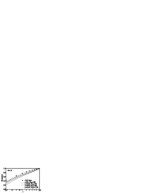
FIG. 3.: The energy profile of a 100 GeV jet, taken from [5].

However, the danger in this is that the value of $R_{\mathrm{sep}}$ is not given to us by the jet definition and could be viewed as a phenomenological parameter that should be tuned to data. In this sense, there is no reason to suppose that the value of $1.3R$ should also describe jets in the far forward region, or jets produced in a completely different reaction, like top quark decays.

One very nice feature of cone algorithms is the apparent ease with which energy corrections can be made. This is because they are purely geometrical, so the amount of out-of-cone showering in the calorimeter for example, can be very easily calculated from the known detector response and the energy inside the cone. Another type of correction that is sometimes applied is for the amount of the jet’s energy that is radiated outside the cone and the amount of energy from the underlying event that sneaks into the cone. When comparing with leading order calculations this may appear straightforward since they do not account for the energy spread of the jet. However, at next-to-leading order, the calculation already includes the fact that some of a jet’s energy is radiated outside the cone, so this should not be corrected for. Furthermore, the underlying event correction is inevitably model-dependent, even when it is measured from data. This is because in some models the jet pedestal is correlated with the jet momentum and direction, while in others it is completely uncorrelated. Thus different experimental procedures such as subtracting the average seen in a cone in minimum bias events or the average seen in a random direction in jet events at the same jet transverse momentum will give results that are interpreted differently in different models. The effect of such assumptions on jet data is discussed in detail in [7]. An experimental test was proposed in [8] that would shed a lot of light on these problems, since it claims to disentangle how correlated the jet activity and pedestal height are.

$k_{\perp}$ Clustering Algorithms

Clustering algorithms have been the main way of defining jets in $\mathrm{e^{+}e^{-}}$ annihilation for many years. They work in a very different way from cone algorithms — instead of globally finding the jet direction, they start by finding pairs of particles that are ‘nearby’ in phase-space and merging them together to form new pseudoparticles. This continues iteratively until the event consists of a few well-separated pseudoparticles, which are the output jets. There is however, no unique definition of ‘closeness’ in phase-space and different definitions define different algorithms. Traditionally invariant mass was used, but this has the disadvantage that it is extremely non-local in angle — if two particles have low enough energy, they will be merged together, regardless of how far apart they are in angle [9]. This can be solved by using as closeness the momentum of the softer particle transverse to the axis of the harder [10], as in the $k_{\perp}$ jet algorithm. This means that, roughly speaking, the algorithm repeatedly merges the softest particle in the event with its nearest neighbour in angle. It has the great theoretical advantage that it allows the phase-space for multiple emission to be factorized in the same way as the QCD matrix elements, allowing analytical parton shower techniques to be used [11], as I describe below.

However, in collisions with incoming hadrons, there are additional particles in the final state that are not associated with hard jets, namely those coming from the hadron remnant and underlying event. For many years this was seen as a barrier to using clustering algorithms in hadronic collisions, as their property of exhaustively assigning every final state particle to a jet is clearly unphysical there. This problem was considered in [12], where it was shown that it could be overcome by introducing an additional particle into the event by hand, parallel to the incoming beams. In the case of the $k_{\perp}$ algorithm, this extra particle can be considered as having infinite momentum. The resulting jet cross-sections are guaranteed to satisfy the factorization theorem, so absolute predictions using p.d.f.s measured in other processes can be made for their values, unlike earlier attempts to solve this problem.

As far as the practical properties of the algorithm are concerned, it is essential for jet algorithms for hadron-hadron collisions to be invariant under longitudinal boosts along the beam direction. A set of longitudinally-invariant $k_{\perp}$-clustering algorithms for hadron-hadron collisions was proposed in [13]. Briefly, the algorithm proceeds as follows:

1. For every pair of particles, define a closeness

   
   

   $\displaystyle d_{ij}=\min(E_{Ti},E_{Tj})^{2}\Delta R^{2},\quad\quad\Delta R^{2}\equiv\Delta\eta^{2}+\Delta\phi^{2}.$

   Note that for small opening angle, $\Delta R\ll 1,$ we have

   
   

   $\displaystyle\min(E_{Ti},E_{Tj})^{2}\Delta R^{2}\approx\min(E_{i},E_{j})^{2}\Delta\theta^{2}\approx k_{\perp}^{2}.$

2. For every particle, define a closeness to the beam particles,

   
   

   $\displaystyle d_{ib}=E_{Ti}^{2}R^{2},$

   where $R$ is an adjustable parameter of the algorithm introduced in [14].

3. If $\min\{d_{ij}\}<\min\{d_{ib}\},$ merge particles $i$ and $j$.

4. If $\min\{d_{ib}\}<\min\{d_{ij}\},$ jet $i$ is complete.

These steps are iterated until a given stopping condition is satisfied, as I discuss in more detail in a moment. Different ways of merging two four-vectors into one define different schemes — the two most common are the “$E$”-scheme (simple four-vector addition) and the “$p_{t}$”-scheme:

$$E_{Tij} = E_{Ti}+E_{Tj},$$

$$\eta_{ij} = \left(E_{Ti}\eta_{i}+E_{Tj}\eta_{j}\right)/E_{Tij},$$

$$\phi_{ij} = \left(E_{Ti}\phi_{i}+E_{Tj}\phi_{j}\right)/E_{Tij},$$

which become equivalent for small opening angle. Although there are some small practical differences, they are not important here.

Depending on what kind of studies one is interested in, different stopping conditions are useful. For inclusive jet studies, one iterates the above steps until all jets are complete [14]. In this case, all opening angles within each jet are $<R$ and all opening angles between jets are $>R$. This means that the resulting jets are very similar to those produced by the cone algorithm, with $R\sim R_{\mathrm{sep}}$. As shown in Fig. 4, this is certainly true of the inclusive jet cross-section, for which the two algorithms are almost indistinguishable at next-to-leading order.

FIG. 4.: The inclusive jet cross-section for central jets with $E_{T}=100$ GeV, as a function of $R$ for the cluster algorithm and $1.35R_{\mathrm{cone}}$ for the cone algorithm, for three different values of the renormalization and factorization scales, $\mu$. The barely discernible pairs of curves are from the cone and cluster algorithms. Taken from [14], where more precise details of the calculation can be found.

It is worth noting that for a relatively soft jet, $d_{ij}$ is its transverse momentum relative to the nearest hard jet, while $d_{ib}$ is $R^{2}$ times its transverse momentum relative to the incoming beams. If $d_{ib}$ is the smaller then the jet is treated as initial-state radiation, giving a resolvable jet, while if it is the larger it is treated as final-state radiation, being merged into the other jet. Thus the value $R=1$ is strongly preferred theoretically, as it treats initial- and final-state radiation on equal footings and would be expected to give smallest higher-order corrections, at least from the dominant logarithmic regions of phase-space. In this sense, the empirical relationship between $R$ and $R_{\mathrm{cone}}$ can be used as an a posteriori justification for using $R_{\mathrm{cone}}=0.7$. The first experimental results using this algorithm were reported in [15].

In many cases, one instead wants to reconstruct exclusive final states, for example in top quark decay. In this case, one iterates the above steps until all jet pairs have $d_{ij}>d_{\mathrm{cut}},$ an adjustable parameter of the algorithm. All complete jets with $d_{ib}<d_{\mathrm{cut}}$ are discarded (merged with the beam remnants). Thus $d_{\mathrm{cut}}$ acts as a global cutoff on the resolvability of emission, initial- or final-state. In this case setting $R=1$ is even more strongly recommended, as in the original algorithm of [13]. One can either fix $d_{\mathrm{cut}}$ a priori, only resolving radiation above the given $k_{\perp}$ cutoff, or adjust it event-by-event to reconstruct a given number of final-state jets.

Although the cluster jets are very similar to the cone jets in terms of the inclusive cross-section, they have several practical advantages. Firstly, the jet overlap problem has completely disappeared — the algorithm unambiguously assigns every particle to a single jet. It does this in a dynamic way, adjusting to the shapes of individual jets, and so performs better than any fixed strategy such as drawing a dividing line half way between the centres or giving all the energy to the higher-energy of the two. One can of course always come up with pathological jet configurations where any given algorithm does not cluster in the way that seems natural, but the relative contribution of such configurations is much smaller for the cluster algorithm than the cone. This means that exactly the same algorithm can be used on hadronic final states with many particles as on partonic final states with one or two, without the need for additional adjustable parameters. Secondly, the cluster algorithm is much less sensitive to perturbations from soft particles than the cone algorithm, which results in smaller hadronization and detector corrections, as well as a reduction in the model-dependence of these corrections. This is because in some sense it pays the most attention to the core of the jet and only merges other neighbouring particles if they are near enough to do so, whereas the cone algorithm, which seeks to maximize the jet energy, does its best to pull in as much neighbouring energy as possible, as illustrated in Fig. 5.

FIG. 5.: The energy profiles of 100 GeV cone and cluster jets, taken from [14]. The cluster jets (labeled “Comb”) have more energy concentrated in the centremost bin, while the cone jets are more diffuse. At the jet edge, $r=R=R_{\mathrm{cone}}=1,$ the trend is reversed — the cluster algorithm ignores energy more than $R$ away so gives a flat background contribution, while the cone algorithm has tried to pull this energy into the jet, leaving a deficit outside.

This feature means that the $k_{\perp}$ cluster algorithm is particularly suited for kinematic reconstruction of particle decays. A detailed Monte Carlo comparison was made in [16] for the cases of top quark reconstruction at Tevatron energy and Higgs boson at LHC energy. The results for the former are shown in Fig. 6

FIG. 6.: Reconstructed three-jet mass distribution of top quark candidates, according to the cluster (solid) and cone (dashed) algorithms, at calorimeter level, for a top quark of nominal mass 150 GeV. Taken from [16].

for the mass of the three-jet combination that minimizes

$\displaystyle\chi^{2}\equiv\left(\frac{m_{\mathrm{jj}}-\langle m_{\mathrm{jj}}\rangle}{\mbox{5 GeV}}\right)^{2}+\left(\frac{m_{\mathrm{jjj}}-m_{\ell\nu\mathrm{j}}}{\mbox{10 GeV}}\right)^{2},$

after the cut $\chi^{2}<3$. The other cuts are described in [16]. The cluster algorithm’s mass distribution is centred on the true value and is much more symmetric than the cone algorithm’s. Also the efficiency of the cluster algorithm is considerably higher, owing to the greater cleanliness of the event reconstruction, so that even though the widths of the two distributions are similar, the cluster algorithm would give a smaller error on the reconstructed mass. Another reason for this greater cleanliness is that the cluster algorithm is somewhat like a cone algorithm with its radius adjusted event-by-event to suit the individual event dynamics — when there are two hard jets near each other the effective radius is small to resolve them well, when they are all far apart it is large, allowing a good measurement of their energies.

Internal Jet Structure

It is clearly important to study the internal structure of jets, both as a test of QCD and to understand the efficiencies, corrections, etc, of jet reconstruction for other studies. In the cone algorithm, the natural way to do this is by studying the spread of energy over various annular radii, as shown in Figs. 3 and 5. In the cluster algorithm, one has the possibility to study the internal structure in a way that is much more like how we believe jets develop — their structure comes not from a general smearing in angle, but by radiating individual partons that give rise to smaller ‘sub-jets’ within the jet. Thus by resolving these sub-jets we can compare their distributions with those predicted by QCD or by Monte Carlo models.

Sub-jets are defined by first running the inclusive version of the algorithm to find a jet. Then the algorithm is rerun starting from only the particles that were part of that jet, stopping when all pairs have

$\displaystyle d_{ij}>y_{\mathrm{cut}}E_{T}^{2},$

where $E_{T}$ is the transverse momentum of the jet and $y_{\mathrm{cut}}$ is an adjustable resolution parameter. For $y_{\mathrm{cut}}\sim 1$ the jet always consists of only 1 sub-jet and for $y_{\mathrm{cut}}\to 0$ every hadron is considered a separate sub-jet, so adjusting $y_{\mathrm{cut}}$ allows us to go smoothly into the hadronization region in a well-defined way and to study the parton$\to$many partons$\to$hadrons transition in great detail. Further details and the first experimental results can be found in [17]. Similar studies have also been performed in $\mathrm{e^{+}e^{-}}$ annihilation [18, 19] and will allow direct comparisons of the two sources of jets.

Of course, sub-jets can also be defined in the cone algorithm, by rerunning using a smaller jet radius. Results of a Monte Carlo comparison are shown in Fig. 7, where it can be seen that the cone algorithm has much larger hadronization correction.

FIG. 7.: The fraction of two-jet events that contain 2, 3, 4, or 5 sub-jets when resolved at a scale $y_{\mathrm{cut}}$ for the cluster algorithm and a radius $r$ for the cone algorithm, at the parton level (solid) and calorimeter level (dotted). Taken from [20].

The reasons for this are discussed in [20].

Calculating Jet Properties

To study QCD, and to understand the corrections and efficiencies of jet reconstruction, we are particularly interested in the internal properties of jets. We have already seen in Walter’s talk [3] that external jet properties such as the transverse momentum spectra, rapidity distributions, dijet mass spectra, etc, are well-described by next-to-leading order QCD calculations. The internal properties that I will be concerned with are things like the energy profile of a jet, jet mass distributions and internal sub-jet structure, which are infrared-finite and can be calculated in perturbation theory. However, owing to the one-to-one correspondence between partons and jets in leading order calculations, the leading non-trivial term is the one given by “next-to-leading” order jet calculations. This means that they suffer all the usual problems with leading order calculations, like large sensitivity to the renormalization scale.

For many of these jet properties, one encounters large logarithmic terms at all orders in perturbation theory and it is essential that these terms are reorganized (“resummed”) into an improved perturbation series. Examples include the energy profile at small angles and the sub-jet structure at small $y_{\mathrm{cut}}$. This is conventionally done by the parton shower approach, either as a Monte Carlo simulation, or analytically.

Parton Showers

The cross-section for multiple emission factorizes in the collinear limit. This means that the production of additional partons close to a jet direction can be described in a time-ordered probabilistic way as a series of $1\to 2$ splittings one after another. In the strongly-ordered limit, in which each splitting is much more collinear than the last, this is guaranteed to reproduce the exact multi-parton matrix element. This strongly-ordered region of phase-space contributes the leading logarithmic contribution to energy-weighted quantities like the energy profile. Thus any parton shower based on sequential collinear emission can predict these properties to leading logarithmic accuracy. It is worth noting that in the strongly-ordered limit, all measures of collinearity, like transverse momentum, virtuality and angle, are completely equivalent — algorithms that use different choices differ only by next-to-leading logarithms.

However, many jet properties are sensitive to soft gluon emission, such as the sub-jet distributions. In this case, it seems at first sight like no probabilistic algorithm could possibly describe the full matrix element. This is because the matrix-element amplitude for any given final-state configuration is the sum of terms in which the gluon is emitted by each external leg, as illustrated in Fig. 8.

FIG. 8.: Soft large-angle gluons cannot resolve the individual colour charges in the jet, so the coherent sum of emission off all the external lines is equivalent to emission by the original parton, imagined to be on-shell, i.e. before the other emission.

Unlike the collinear case, all of these contribute to the leading logarithm and when taking the square of the sum the interference terms can be both positive and negative. Therefore it looks like we have to abandon the idea of describing the production of soft gluons in terms of independent probabilistic $1\to 2$ splittings.

However the fact that radiation from all the different emitters is coherent, a simple consequence of gauge invariance, comes to the rescue. It means that, after averaging over the relative azimuths of different emissions, the emission of any given soft gluon can be attributed to a single coloured line somewhere in the diagram, either external, or internal but imagined to be on-shell [23]. The fact that the emission probability from an internal line is what it would be if it was on-shell results in the famous angular ordering condition [24], namely that large angle emission should be treated as occuring earlier than smaller angle emission. This is the basis of coherent parton shower algorithms.

It is important to note that this is not the same as using a standard virtuality-ordered algorithm and disallowing disordered emission, although claims are often made to the contrary. For example, in the configuration of Fig. 8, the total gluon emission probability is non-zero and proportional to $C_{F},$ the colour charge of a quark, whereas the veto algorithm would simply disallow all soft large-angle emission from this system.

Many of the most important next-to-leading logarithmic contributions can be incorporated by simple modifications to the leading logarithmic coherence-improved algorithm. A well-known example is the argument of the running coupling — large sub-leading corrections can be summed to all orders simply by using transverse momentum.

Emission from initial-state coloured partons can also be treated in the same way. Collinear emission is responsible for the scaling violations in the parton distribution functions. This means that the input set of p.d.f.s can be used to guide the collinear emission and ensure that the distributions produced are the same as those used in theoretical calculations. This allows a ‘backwards’ evolution algorithm to be used [25] with evolution starting at the hard interaction and working downwards in scale back towards the incoming hadron. Partons produced by initial-state radiation subsequently undergo final-state showering. The coherence of radiation from different sources can again be incorporated by choice of the evolution scale, at least for not too small momentum fractions. In this case the appropriate variable is the product of the opening angle and the emitter’s energy [27].

So far I have described how the parton shower evolves, but it also needs a starting condition to evolve from. This is particularly important for interjet properties, as well as for setting the whole scale of the subsequent evolution. It is provided by the lowest order matrix element for the process under consideration — jet production, prompt photon, top quark production and decay, or whatever. As shown in [28], the coherence of radiation from the various emitters plays an important rôle here too. Each hard process can be broken down into a number of ‘colour flow’ diagrams, which control the pattern of soft radiation in that process. To leading order in the number of colours, $N_{c},$ gluons can be considered as colour-anticolour pairs and a unique ‘colour partner’ can be assigned to each parton for each colour flow. After azimuthal averaging, radiation from each parton is limited to a cone bounded by its colour connected partner, as illustrated for a particularly simple case in Fig. 9.

FIG. 9.: Feynman (left), colour flow (centre) and cmf frame (right) diagrams of $\mathrm{q\bar{q}\to q^{\prime}\bar{q}^{\prime}}$ showing the radiation cones of each parton. Most processes have many different colour flows.

It is important to note that although the radiation inside the cone around each parton is modeled as coming from that parton, it is the coherent sum of radiation from all emitters in the event even the internal lines, a point that I shall return to later.

Violations of this picture come from two main sources — colour-suppressed terms and semi-soft terms. $1/N_{c}$ is not such a small expansion parameter so one might expect non-leading colour terms to be a very important correction. However, they tend to be also dynamically suppressed, since they are non-planar, and neglecting them is generally a good approximation. One can however find special corners of phase-space in which no parton shower algorithm based on the large-$N_{c}$ limit could be expected to be reliable [29]. The colour-suppressed terms are generally negative and have not successfully been incorporated into a probabilistic Monte Carlo picture. The semi-soft corrections arise simply from the fact that the emission cones are derived in the limit of extremely soft emission that does not disturb the kinematics of the event at all, while harder emission makes the emitters recoil, disturbing their radiation patterns. Both of these effects mean that the initial conditions used in most implementations of coherent parton showers are actually too strong, since they prevent emission in regions where it is suppressed but not absent in the full calculation (i.e. outside the cones).

Monte Carlo Parton Showers

Monte Carlo shower algorithms implement the probabilistic interpretation in a very literal way, using a random number generator. They give fully exclusive distributions of all final-state properties with unit weight, meaning that any given configuration occurs with the same frequency as in nature. The relevant jet properties can be directly measured from the produced particles, exactly as in the experimental procedure.

The available models were thoroughly reviewed in [30], so I only make a few brief comments about each.

ISAJET [31] implements a virtuality-ordered collinear parton shower algorithm for both initial- and final-state evolution. It does not include any account of coherence. It is specific to hadron-hadron collisions, so its parameters can be freely tuned to improve the fit to data.

PYTHIA [32] also implements a virtuality-ordered collinear parton shower algorithm. In the case of final-state radiation, this is coherence-improved by disallowing emission with disordered opening angles. Coherence is now incorporated into the initial conditions for the initial-state radiation (this is called ‘PYTHIA+’ below and is now the default), but not within the evolution itself. The parameters are those tuned to $\mathrm{e^{+}e^{-}}$ annihilation so the model is already well-constrained and predictive for hadron-hadron collisions.

HERWIG [33] implements a complete coherence-improved parton shower algorithm for both initial- and final-state evolution, incorporating azimuthal correlations both within and between jets. The implementation is sufficiently precise that in limited regions of phase-space it is reliable to next-to-leading logarithmic accuracy, and HERWIG’s $\Lambda$ parameter can be related to $\Lambda_{\overline{\mathrm{MS}}}$ [34]. The parameters are again tuned to $\mathrm{e^{+}e^{-}}$ and DIS data making the model highly predictive.

ARIADNE [35] is a new Monte Carlo event generator that has only recently become available for hadron-hadron collisions, although it has been very successful in describing $\mathrm{e^{+}e^{-}}$ and DIS data. It fully implements colour coherence, but in a completely different way to that described above, being based on the colour dipole cascade model [22]. It makes no separation into initial- and final-state radiation, instead modeling the emission from the whole system in a coherent way. Its parameters are also tuned to $\mathrm{e^{+}e^{-}}$ and DIS data.

The issue of coherence has become paramount in describing $\mathrm{e^{+}e^{-}}$ data, and models that do not implement it, at least approximately, are completely ruled out (see for example [36] and references therein). They are also strongly disfavoured in DIS. Data from the collider are now sufficiently precise that coherence effects can also be studied there. Fig. 10 shows the results of a recent CDF study [37] of the distribution of the softest jet in three jet events.

FIG. 10.: The rapidity distribution of the third-hardest jet in multi-jet events, taken from [37].

Only the models incorporating coherence, HERWIG and the updated PYTHIA, can account for the data. It is possible that a similar interpretation could be made of the sub-jet data presented in [17], although further study is needed to confirm this.

Hard Parton Shower Emission

By construction, coherence-improved shower algorithms reproduce the exact matrix element in the soft and collinear limits. Soft here means relative to the hardest scale in the event — a jet of 50 GeV or so could be considered soft in the context of top quark production for example. However, jet cuts always pull us away from the soft and collinear regions since they require the emission to be resolvable. For example, the cross-section for ‘Mercedes’ events, with three jets of equal transverse momentum evenly spaced in azimuth, is not completely negligible and since this is so far from any singular regions, we should certainly worry how well parton shower algorithms will reproduce it. There are two separate worries — whether there are phase-space regions that the algorithm does not populate and whether it is a good enough approximation in the regions is does populate.

The accuracy of fixed-order matrix elements is complementary to that of parton showers — they are exact for hard well-separated jets (to leading order in $\alpha_{s}$), but do not correctly account for multiple emission effects, so become increasingly unreliable if the cutoffs are made very small. It is natural to hope that the two approaches can be combined to yield a single algorithm that is uniformly reliable for hard and soft emission, collinear and well-separated. Several phenomenological attempts have been made in the past, but these generally suffer a variety of problems. Firstly, it is essential that if the phase-space region is divided into two parts then they are smoothly matched at the boundary to prevent double-counting or under-counting. Ideally the boundary itself should be an arbitrary parameter so that one can explicitly check that varying it does not affect the output distributions. It is worth noting that for this to be true, it is incorrect to use the exact leading order matrix element, as a form factor must be introduced even within the hard region. Many algorithms work by correcting the first emission to reproduce the hard matrix element. However, the choice of ordering variable is scheme-dependent and so therefore is the definition of which emission is first. This problem is particularly severe in angular-ordered parton shower algorithms, where there are often several soft large-angle emissions before the hardest emission in the jet. If one nevertheless just corrects the first emission, one obtains a hard limit that is dependent on the soft infrared cutoff of the algorithm, which is clearly unphysical.

These problems were discussed in [38], where self-consistent algorithms were proposed for correcting both deficiencies — filling empty regions of phase-space and correcting the distributions of all hard emission (not just the first) within the parton shower region. There is no conceptual barrier to applying them to arbitrary hard processes, such as top quark production and decay, and it would be straightforward to do so in an algorithm specifically designed with this in mind. However, it has proved rather tricky to weave them into the existing HERWIG algorithm and this has so far only been done for the simplest processes, $\mathrm{e^{+}e^{-}\to q\bar{q}}$ and DIS, $\mathrm{eq\to eq}$. Results for the latter are shown in Fig. 11.

FIG. 11.: The transverse momentum flow in the $\gamma^{*}\mathrm{p}$ centre-of-mass frame of DIS events at small $x$, taken from [39], data from [40]. The first three curves are without detector acceptance and the dot-dash is the third after including the acceptance.

The hard correction, i.e. the filling of empty phase-space regions is an important correction, while the soft correction, within the parton-shower phase-space makes very little difference. The same is also true in $\mathrm{e^{+}e^{-}}$. This can be interpreted as meaning that although HERWIG’s parton shower algorithm does not fill the whole of phase-space owing to its over-strict implementation of the angular-ordering initial condition, it is a good approximation in the regions it does fill.

It seems plausible that these corrections would fix the problems for top quark production and decay events reported in [41] and in Stephen Parke’s talk [42], but we have not yet been able to explicitly check this.

Azimuthal Decorrelation

In the last couple of years there have been several proposed tests of ‘non-DGLAP’ evolution, i.e. quantities for which the collinear evolution described above is insufficient, as discussed in the talk by Vittorio del Duca [43]. Although some of these are certainly sensitive to new small-$x$ dynamics, many can be reliably predicted using coherence-improved evolution.

One such example is the decorrelation in azimuth of jet pairs as the rapidity interval between them increases. In the BFKL framework, this is attributed to emission from the $t$-channel exchanged gluon, as illustrated in Fig. 12 for a simple example, $\mathrm{qq^{\prime}\to qq^{\prime}},$ chosen because it has a single colour flow.

FIG. 12.: BFKL ladder (left), full emission pattern (centre) and leading-$N_{c}$ emission pattern (right) for small angle $\mathrm{qq^{\prime}}$ scattering, contributing to the azimuthal decorrelation of the resulting jets. In the full case, emission from each quark is confined to its small forward cone and there is emission from the internal gluon, while in the leading-$N_{c}$ case each quark emits everywhere except its small backward cone and there is no other emission.

The full emission pattern of this system consists of emission proportional to $C_{F}$ inside small cones of opening angle $\theta_{s},$ the scattering angle and proportional to $C_{A}$ in the remainder of the solid angle. However, a coherence-improved parton shower would describe this situation as two colour lines, each of which have been scattered through almost $180^{\circ}$. Thus each quark emits proportional to $C_{F}$ into a ‘cone’ of opening angle $180^{\circ}\!-\theta_{s}$ and, apart from the difference between $C_{A}$ and $2C_{F},$ a $1/N_{c}^{2}$ correction, it reproduces the full emission pattern. Thus to leading order in the number of colours, coherence-improved parton showers include soft emission from this internal line and should reproduce the full QCD result for azimuthal decorrelations.

Analytical Parton Showers

The probabilistic parton shower framework described above can also be used for analytical calculations. In this case, one sets up a probabilistic evolution equation for how the quantity of interest, for example the distribution of sub-jets, changes as a function of either the jet $p_{t}$ or resolution scale. This gives integro-differential equations that, with appropriate boundary conditions, can be solved analytically. However, this can only be done for experimental observables in which the phase-space for multiple resolved emission factorizes. In the case of sub-jets this essentially requires that the resolution variable be of $k_{\perp}$ type. So far, only one calculation of this type has been made for hadron-hadron collisions (although there are several for $\mathrm{e^{+}e^{-}}$ and DIS), for the average number of sub-jets resolved in an inclusive jet [44]. The result is shown in Fig. 13 and is compared to D0 data in [17].

FIG. 13.: The average number of sub-jets in a central 100 GeV jet, taken from [44].

The increasing importance of the all-orders resummation of next-to-leading logarithmic terms at small $y_{\mathrm{cut}}$ can be clearly seen.

Hadronization

The process by which coloured partons are confined into hadrons is not understood at a fundamental level at present, so phenomenological models must be used. The dynamics of the parton shower are preconfining, meaning that partons tend to end up close, in both phase-space and real-space, to their colour-connected partners. This suggests that hadronization is a fairly local process, taking place in the spatial regions between (but near to) the final-state partons. The string and cluster models used in PYTHIA and HERWIG respectively both implement this idea and both give good fits to $\mathrm{e^{+}e^{-}}$ data. Like their parton shower algorithms, the model parameters are strongly constrained by $\mathrm{e^{+}e^{-}}$ data, making them highly predictive for hadron-hadron collisions. The independent fragmentation model, in which single partons decay to hadrons according to longitudinal phase-space with no account of colour connections, is already ruled out by $\mathrm{e^{+}e^{-}}$ data.

Owing to lack of time in the talk and space in the proceedings, I can do no more than mention a new area that is sure to grow in the near future, the analytical calculation of hadronization corrections. Several different approaches appear to be converging on the result that perturbation theory, suitably modified, is more powerful than we thought and may even be capable of predicting hadron-level cross-sections. The introduction of an effective running coupling that is integrable at low momenta [45] alone may be sufficient to calculate the dominant corrections to infrared-finite quantities, although the factorization this implies [46] has been questioned in renormalon-based approaches [47, 48]. More details can also be found in George Sterman’s talk [49].

Conclusion

As I have stressed throughout the talk, jets are not fundamental objects in QCD, but are artificial event properties defined by hand. Different definitions have good and bad points and the results will be a function of these definitions. We need reliable methods to calculate these event properties from the fundamental objects of perturbative QCD, quarks and gluons.

Cone-type jet algorithms are simple in principle, but turn out to be complicated in practice, owing to jet overlap problems. Cluster-type algorithms are more complicated to define, but turn out to be simple in practice, since exactly the same algorithm can be used for one or two partons as on the hadron-level or detector-level final state. The $k_{\perp}$ cluster algorithm has a variety of practical and theoretical advantages both for jet physics and for event reconstruction.

For jet properties, very few analytical calculations are available, particularly in the important region of small resolution parameters, but this is expected to improve in the future. Modern coherence-improved Monte Carlo models are very sophisticated implementations of perturbative QCD plus very constrained models of hadronization and are highly predictive for hadron-hadron collisions. However, there are areas in which they need to be improved, most notably in matching parton showers with exact matrix elements to improve the description of very hard emission.

It is clear that many areas outside the standard QCD arena are becoming increasingly reliant on jet physics. For example the error on the top mass will soon become dominated by the treatment of gluon radiation and it will become absolutely essential to consider the problems discussed in this talk. Namely, how can the present jet definition and modeling be improved upon?

REFERENCES

- [1] S.D. Ellis, talk presented in the parallel session on jets, unpublished.
- [2] A. Bhatti, these proceedings; F. Nang, these proceedings.
- [3] W. Giele, these proceedings.
- [4] J. Huth et. al., in Proc. Summer Study on High Energy Physics, Snowmass, 1990.
- [5] S.D. Ellis, Z. Kunszt and D.E. Soper, Phys. Rev. Lett. 69 (1992) 3615.
- [6] CDF Collaboration, Phys. Rev. Lett. 70 (1993) 713.
- [7] S.D. Ellis, in Proc. 28th Rencontres de Moriond, 20–27 March 1993.
- [8] G. Marchesini and B.R. Webber, Phys. Rev. D38 (1988) 3419.
- [9] N. Brown and W.J. Stirling, Phys. Lett. B252 (1990) 657; Z. Phys. C53 (1992) 629; N. Brown, J. Phys. G17 (1991) 1561.
- [10] S. Catani, et. al., Phys. Lett. B269 (1991) 432.
- [11] S. Catani, Yu.L. Dokshitzer, F. Fiorani and B.R. Webber, Nucl. Phys. B377 (1992) 445; Nucl. Phys. B383 (1992) 419.
- [12] S. Catani, Yu.L. Dokshitzer and B.R. Webber, Phys. Lett. B285 (1992) 291; B.R. Webber, J. Phys. G19 (1993) 1567.
- [13] S. Catani, Yu.L. Dokshitzer, M.H. Seymour and B.R. Webber, Nucl. Phys. B406 (1993) 187.
- [14] S.D. Ellis and D.E. Soper, Phys. Rev. D48 (1993) 3160.
- [15] K.C. Frame, in Proc. DPF94, Albuquerque, 2–6 August, 1994.
- [16] M.H. Seymour, Z. Phys. C62 (1994) 127.
- [17] R.V. Astur, these proceedings.
- [18] OPAL Collaboration, Z. Phys. C63 (1994) 363.
- [19] ALEPH Collaboration, Phys. Lett. B346 (1995) 389.
- [20] M.H. Seymour, in Proc. 28th Rencontres de Moriond, 20–27 March 1993.
- [21] I.G. Knowles, Nucl. Phys. B310 (1988) 571.
- [22] G. Gustafsson and U. Pettersson, Nucl. Phys. B306 (1988) 746.
- [23] Yu.L. Dokshitzer, V.A. Khoze, A.H. Mueller and S.I. Troyan, Basics of Perturbative QCD, Editions Frontières, 1991.
- [24] G. Marchesini and B.R. Webber, Nucl. Phys. B238 (1984) 1.
- [25] T. Sjöstrand, Phys. Lett. bf B157 (1985) 321.
- [26] G. Marchesini and B.R. Webber, Nucl. Phys. B386 (1992) 215.
- [27] G. Marchesini and B.R. Webber, Nucl. Phys. B310 (1988) 461.
- [28] R.K. Ellis, G. Marchesini and B.R. Webber, Nucl. Phys. B286 (1987) 643.
- [29] Yu.L. Dokshitzer, V.A. Khoze and S.I. Troyan, The Azimuthal Asymmetry of QCD Jets as Experimentum Crucis for the String Fragmentation Picture, Leningrad preprint 1372, 1988.
- [30] I.G. Knowles and S.D. Protopopescu, in Proc. Workshop on Physics at Current Accelerators and Supercolliders, Argonne, June 2–5, 1993.
- [31] F.E. Paige and S.D. Protopopescu, in Proc. Summer Study on the Physics of the Superconducting Super Collider, Snowmass, 1986.
- [32] T. Sjöstrand, Computer Phys. Commun. 82 (1994) 74.
- [33] G. Marchesini et. al., Computer Phys. Commun. 67 (1992) 465.
- [34] S. Catani, G. Marchesini and B.R. Webber, Nucl. Phys. B349 (1991) 635.
- [35] L. Lönnblad, Computer Phys. Commun. 71 (1992) 15.
- [36] M. Schmelling, Physica Scripta 51 (1995) 683.
- [37] CDF Collaboration, Phys. Rev. D50 (1994) 5562.
- [38] M.H. Seymour, hep-ph/9410414, to appear in Computer Phys. Commun.
- [39] M.H. Seymour, LU TP 94–12, gls0258, contributed to the 27th International Conference on High Energy Physics, Glasgow, U.K., 20–27 July 1994.
- [40] H1 Collaboration, Z. Phys. C63 (1994) 377.
- [41] L. Orr, T. Stelzer and W.J. Stirling hep-ph/9412294; hep-ph/9505282.
- [42] S.D. Parke, these proceedings.
- [43] V. del Duca, these proceedings.
- [44] M.H. Seymour, Nucl. Phys. B421 (1994) 545.
- [45] Yu.L. Dokshitzer and B.R. Webber, hep-ph/9504219.
- [46] R. Akhoury and V.I. Zakharov, hep-ph/9504248.
- [47] P. Nason and M.H. Seymour, hep-ph/9506317.
- [48] G.P. Korchemsky and G. Sterman, Nucl. Phys. B437 (1995) 415; hep-ph/9505391, contributed to 30th Rencontres de Moriond, 19–25 March, 1995.
- [49] G. Sterman, these proceedings.