hep-ph/9506346 THU-95/16

The Feynman-Schwinger representation is used to study the behavior of solutions of scalar QED in (2+1) dimensions. The limit of zero photon mass is seen to be smooth. The Bethe-Salpeter equation in the ladder approximation also exhibits this property. They clearly deviate from the behavior in the nonrelativistic limit. In a variational analysis we show that this difference can be attributed to retardation effects of relativistic origin.

PACS numbers: 11.15.Tk, 11.10.St, 03.65.Ge

Keywords:	gauge invariance, nonperturbative scalar QED2+1, bound states,
	nonrelativistic limit, Feynman-Schwinger representation, Bethe-Salpeter
	equation, logarithmic confinement.

Accepted for publication in Physics Letters B

An important issue in the description of relativistic composite systems is to find a reliable and practical formalism that is consistent with known limiting cases and the underlying symmetries of the system at hand. The Feynman-Schwinger representation (FSR) [1–7] offers a nonperturbative description which is consistent with both gauge and Lorentz invariance. Furthermore, the formalism was shown to satisfy the correct static and nonrelativistic limits. In this formulation all ladder and crossed graphs are summed up, while the inclusion of valence particle loops, self energies and vertex corrections is feasible as well. Moreover, the FSR is well suited for the study of nonabelian confining theories such as QCD, since vacuum condensates can easily be accounted for via the cumulant expansion [3–5]. These considerations indicate that the FSR is an appealing alternative to the celebrated Bethe-Salpeter equation (BSE).

In this letter we apply the FSR to (2+1) dimensional scalar QED (sQED₂₊₁) in the two-body sector. Our interest in this theory is twofold. First we consider it to be an excellent playground to study the FSR in the equal mass case, since the theory is UV finite in the two-body sector in contrast with the situation in (3+1) dimensions. Secondly, it has been proven that compactified quenched spinor QED₂₊₁ is linear confining for all values of the charge [8, 9]. Since the spin of the valence particles is usually not considered to be essential for the mechanism behind confinement, one may hope to learn something about the confinement mechanism in this abelian case. In this work however, we will focus on the restoration of gauge invariance.

In order to avoid IR problems we introduce a photon mass $\mu$ in the theory and study the limit $\mu\rightarrow 0$. In this limit we may compare the FSR-results with those of the BSE in the ladder approximation and the Schrödinger equation. The $\mu$ dependence can readily be found in the latter case. Taking the one meson exchange contribution as driving force between 2 charges with mass $m$, we have in 2 spatial dimensions:

$$\left(-\frac{1}{m}\Delta-\frac{e^{2}}{2\pi}K_{0}(\mu r)\right)\psi(r)=-E_{B}\psi(r)$$ (1)

As $\mu\rightarrow 0$ the modified Bessel function $K_{0}(\mu r)$ behaves as $-{\rm log}(\mu r)$, which leads to the well known result of a logarithmic confining Coulomb potential in 2 spatial dimensions after an (infinite) energy shift. This interaction causes $E_{B}$ to diverge as $-\mbox{$\frac{e^{2}}{2\pi}$}{\rm log}(\mu/e\sqrt{m})$, at least for the low lying states.

Let us now turn to the sQED₂₊₁ case. We consider 2 scalar particles with mass $m$, minimally coupled to the massive photon field $A_{\mu}$. The Euclidean action for this theory is:

$$S=\int{\rm d}^{3}x\left[\left|(\partial_{\mu}-{\rm i}eA_{\mu})\phi\right|^{2}+m^{2}|\phi|^{2}+\mbox{$\frac{1}{4}$}F_{\mu\nu}^{2}+\mbox{$\frac{1}{2}$}\mu^{2}A_{\mu}^{2}+\mbox{$\frac{1}{2}$}\xi^{-1}(\partial_{\mu}A_{\mu})^{2}\right]$$ (2)

The parameter $\xi$ takes care of the gauge fixing when we restore gauge invariance by taking the limit $\mu\rightarrow 0$.

The object under study is the gauge invariant 4-point function of the theory, defined as the transition matrix element between the initial state $\Psi_{\rm i}(x,\bar{x})=\phi^{\dagger}(x)P(x,\bar{x})\phi(\bar{x})$ and the final state $\Psi_{\rm f}(y,\bar{y})=\phi(y)P(y,\bar{y})\phi^{\dagger}(\bar{y})$:

$$G(x,\bar{x},y,\bar{y})=\int{\cal D}\phi\;{\cal D}A_{\mu}\;\Psi_{\rm f}(y,\bar{y})\;\Psi_{\rm i}(x,\bar{x})\;{\rm e}^{-S}$$ (3)

The wavefunctions $\Psi_{\rm i}$ and $\Psi_{\rm f}$ are defined in a gauge invariant fashion by means of the parallel transporter $P(x,y)\equiv\exp[-{\rm i}e\int_{x}^{y}{\rm d}z_{\mu}A_{\mu}(z)]$. Next the valence field $\phi$ is integrated out and the resulting determinant is set to unity. The latter amounts to neglecting all $\phi$-loops. It was shown in [1] that the resulting ‘quenched’ Greens’ function can be written in the following form:

$$G(x,\bar{x},y,\bar{y})=\int_{0}^{\infty}{\rm d}s\int_{0}^{\infty}{\rm d}\bar{s}\int({\cal D}z)_{xy}({\cal D}\bar{z})_{\bar{x}\bar{y}}\;{\rm e}^{-K\left[\{z\},s\right]-K\left[\{\bar{z}\},\bar{s}\right]}\left\langle W_{\{z,\bar{z}\}}\right\rangle$$ (4)

where the path integral $\int({\cal D}z)_{xy}$ is a quantummechanical one, subject to the condition of fixed endpoints: $z(0)=x$ and $z(1)=y$. The functional $K$ is the action of a free relativistic point particle with fixed eigentime $s$ [11]:

$$K[\{z\},s]=m^{2}s+\frac{1}{4s}\int_{0}^{1}{\rm d}\tau\;\dot{z}_{\mu}^{2}(\tau)$$ (5)

The Wilson-loop $\left\langle W_{\{z,\bar{z}\}}\right\rangle$ can be computed exactly in the $U(1)$-case considered here:

$$\left\langle W_{\{z,\bar{z}\}}\right\rangle = \left\langle\exp\left[-{\rm i}e\oint_{C}{\rm d}w_{\mu}A_{\mu}(w)\right]\right\rangle_{A_{\mu}}$$ (6)

$$= \exp\left[-\mbox{$\frac{1}{2}$}e^{2}\oint_{C}{\rm d}v_{\mu}\oint_{C}{\rm d}w_{\nu}\Delta_{\mu\nu}(v-w)\right]$$ (7)

$\left\langle W_{\{z,\bar{z}\}}\right\rangle$ is known to be an order parameter of the deconfinement transition in pure gauge theories [10, 11]. The variables $v$ and $w$ in (6) and (7) both run along the whole closed contour $C$ formed by the lines $x\bar{x}$ and $y\bar{y}$ and the paths $\{z\}$ and $\{\bar{z}\}$. Any longitudinal term vanishes identically in (7). The nonvanishing transverse component of $\Delta_{\mu\nu}$ is given by: $\Delta_{\mu\nu}(r)=\delta_{\mu\nu}{\rm e}^{-\mu r}/4\pi r\equiv\delta_{\mu\nu}\Delta(r)$. It can be shown that since there is no ordering of $v$ and $w$ present in (7), it sums up all ladder, crossed ladder, self energy and vertex correction graphs with the appropriate weights. Comparing the FSR to quenched lattice gauge calculations, the calculation of (4) can obviously be carried out in a numerically more accurate way since the occurring path integrals are quantummechanical ones.

Here we wish to concentrate on the ladder and crossed graphs only and we therefore restrict $w$ and $v$ to opposite sides of the contour. The bound state spectrum of the thus obtained expression is studied by considering the asymptotic spectral decomposition of $G$:

$$G(T)=\lim_{T\rightarrow\infty}\sum_{n}c_{n}\exp(-E_{n}T)\hskip 42.67912pt(T\equiv\mbox{$\frac{1}{2}$}(y_{3}+\bar{y}_{3}-x_{3}-\bar{x}_{3}))$$ (8)

and its logarithmic derivative $L(T)=-\left[\frac{{\rm d}}{{\rm d}T}G(T)\right]/G(T)$. According to (8), $L(T)$ is expected to approach the mass of the ground state $E_{0}$ as $T\rightarrow\infty$. In practice we approximated the path integral (4) by a finite product of $N-1$ integrals:

$$\int({\cal D}z)_{xy}\longrightarrow\left(\frac{N}{4\pi s}\right)^{3N/2}\;\prod_{i=1}^{N-1}\int{\rm d}^{3}z_{i}$$ (9)

with the constraints $z_{0}=x$ and $z_{N}=y$. The normalization factor in (9) is not irrelevant since it contains $s$ which is integrated over. The functionals $K$ and $V\equiv\log\left\langle W\right\rangle$ are discretized as follows:

$$K[\{z\},s] \longrightarrow m^{2}s+\frac{N}{4s}\sum_{i=1}^{N}\left(z_{i}-z_{i-1}\right)^{2}$$ (10)

$$V[\{z,\bar{z}\}] \longrightarrow$$

$$\hskip 28.45274pte^{2}\sum_{i,j=1}^{N}\left(z_{i}-z_{i-1}\right)\cdot\left(\bar{z}_{j}-\bar{z}_{j-1}\right)\Delta\left(\mbox{$\frac{1}{2}$}\left(z_{i}+z_{i-1}-\bar{z}_{j}-\bar{z}_{j-1}\right)\right)$$ (11)

Here we adopted the Weyl ordering prescription for noncommuting operators, leading to the midpoint discretization in (11). Our calculations were checked on the convergence with respect to the value of $N$ and usually $N=30$ was found to be sufficiently large to detect no $N$-dependence within statistical errors. We projected $G$ on the eigenstates of total and angular momentum $\left|{\bf P},m\right\rangle$ but due to the nonlocality in (11) this did not imply that the degrees of freedom associated with the symmetries (${\bf P}$, $L^{2}$) could be integrated out. The logarithmic derivative $L(T)$ can be symbolically written as a statistical average (here we denote the set of integration variables $(s$, $\bar{s}$, $\{z_{i}\}$, $\{\bar{z}_{i}\})$ shorthandedly as $Z$):

$$L=\frac{\int\!{\cal D}Z\left(K^{\prime}[Z]-V^{\prime}[Z]\right){\rm e}^{-K[Z]+V[Z]}}{\int\!{\cal D}Z\;{\rm e}^{-K[Z]+V[Z]}}$$ (12)

where the prime stands for analytical differentiation with respect to $T$. We performed Metropolis Monte Carlo calculations of this object by averaging $K^{\prime}[Z]-V^{\prime}[Z]$ over an ensemble generated by $\exp\left(-K[Z]+V[Z]\right)$.

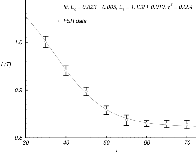
Figure 1: Logarithmic derivative $L(T)$ as a function of the time $T$ for $e^{2}=2.5m$ and $\mu=10^{-3}m$. The solid line is a fit of the data to the form (8).

In Fig. 1 we present results of calculations of $L(T)$ for the case $e^{2}=2.5m$ and $\mu=10^{-3}m$. It is clear that $L(T)$ approaches a constant for large $T$ and a fit of the data to the form (8) allows one to get an accurate result (within 1%) for $E_{0}$ and in principle even a good indication (within 5%) of the first excited state. Note that we are able to do calculations at arbitrary large $T$ since spacetime is not discretized in the FSR approach. This is in sharp contrast with lattice calculations where spacetime is necessarily finite. Besides that, the accuracy of our results is high as compared to lattice calculations [10].

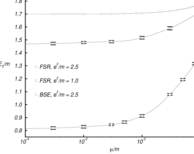
Figure 2: Mass $E_{0}$ of the ground state for sQED₂₊₁ as a function of the photon mass $\mu$. The lines are just drawn to guide the eye. Any logarithmic dependence of $E_{0}$ on $\mu$ would show up in this figure as a straight nonhorizontal line.

In Fig. 2 we display the mass of the ground state obtained with this procedure, as a function of $\mu$ for two different values of the coupling constant $e^{2}$. Clearly the limit $\mu\rightarrow 0$ is a smooth one and we are able to restore gauge invariance in this way. Hence, no logarithmic confinement is found in (2+1) dimensions as long as the mass of the charged particles is kept finite. From these studies we furthermore find that for each $\mu$ there is a finite critical coupling constant where $E_{0}=0$. For $\mu/m=0.1$ this critical coupling constant was determined to be $e_{\rm crit}^{2}/m=6.0\pm 0.5$. At this point the vacuum becomes degenerate in view of these zero mass two-particle bound states.

To get some insight on the absence of the logarithmic confinement in the relativistic case we may study the BSE [12, 13, 16] in the ladder approximation for this theory. In the CM system where $P_{\rm tot}=\left({\bf 0},\sqrt{s}\right)$ it takes on the following form:

$$\Phi(p)=\frac{e^{2}}{(2\pi)^{3}}\int{\rm d}^{3}q\;V(p,q)\;G_{0}(q)\;\Phi(q)$$ (13)

with

$$V(p,q)=\frac{s+(p+q)^{2}}{(p-q)^{2}+\mu^{2}}\hskip 19.91684pt{\rm and}\hskip 19.91684ptG_{0}(q)=\frac{1}{(m^{2}-\mbox{$\frac{1}{4}$}s+q^{2})^{2}+sq_{3}^{2}}$$ (14)

After Wick rotation [14] the momenta in (13) and (14) can be taken Euclidean. The solutions to (13) were constructed by expanding $\Phi$, $V$ and $G_{0}$ on the basis of $O(3)$ spherical harmonics $Y_{lm}(\Omega_{3})$ and truncating the resulting infinite set of coupled one-dimensional integral equations at a certain $l_{\rm max}$. Truncation at $l_{\rm max}=2$ was sufficient to get very accurate results. Further details of this procedure will be published elsewhere. In Fig. 2 the result of the calculations for $e^{2}=2.5m$ are indicated by the diamonds. As compared to the FSR result, the BSE solutions show much less binding. This is a general feature of all our calculations and it is particularly striking for strong couplings. We are led to conclude that the crossed ladder diagrams give a very significant contribution to the binding energy of the system considered here. The limit $\mu\rightarrow 0$ is seen to be smooth as well and we can safely remove the IR cut-off this way.

One may address the question what mechanism is responsible for the smoothness of the limit $\mu\rightarrow 0$ in the relativistic calculations. It is generally known that both the BSE and the FSR have the correct nonrelativistic limit and besides that, it is rather remarkable that such a global feature as this logarithmic divergence does not persist when one considers a relativistic theory. These considerations raise the question how the nonrelativistic limit is being reached in this case. For this purpose we carried out a variational analysis of the BSE for a $g\phi^{3}_{2+1}$-theory. It is convenient to introduce the nonrelativistic coupling constant $\lambda=g^{2}/4m^{2}$ which enters the corresponding Schrödinger equation. We verified that relativistically this case behaves smooth as well for $\mu\rightarrow 0$, while it becomes identical to sQED₂₊₁ in the nonrelativistic limit. Our trial function used:

$$\phi_{\rm trial}({\bf r},t)=\exp\left[-\mbox{$\frac{1}{2}$}\alpha^{2}r^{2}\right]\exp\left[-\mbox{$\frac{1}{2}$}\beta^{2}t^{2}\right]$$ (15)

with variational parameters $\alpha$ and $\beta$, is particularly suited for evaluating the various matrix elements analytically. Nonrelativistically we expect $\alpha\sim{\cal O}\left(\sqrt{E_{B}/m}\right)\gg\beta\sim{\cal O}\left(E_{B}/m\right)$. Applying the Rayleigh-Ritz variational principle to the energy functional $s(\alpha,\beta)$ indeed yields this property up to multiplicative logarithmic corrections. The nonrelativistic limit is obtained by letting $m/\mu\rightarrow\infty$ and at the same time $\lambda/\mu\rightarrow 0$, while keeping their product $\zeta=m\lambda/\mu^{2}$ constant. In this region the wavefunction becomes independent of the relative time $t$ and as a result the Schrödinger predictions are obtained. We find in particular that for

$$\frac{\lambda}{m}\log^{2}(m/\lambda)\ll\zeta^{-1}\ll 1$$ (16)

the binding energy $E_{B}=\left(m^{2}-\mbox{$\frac{1}{4}$}s\right)/m$ goes as $\sim\mbox{ $\frac{1}{4\pi}$}\lambda\log\zeta$. Hence in this region the logarithmic divergence of the Schrödinger analysis is recovered. We see however that $E_{B}$ only exhibits this logarithmic dependence on the photon mass $\mu$ as long as $\zeta$ is kept at a fixed value and $m\rightarrow\infty$ so that the condition (16) is satisfied. Taking on the other hand $m$ large but fixed and letting $\mu\rightarrow 0$, we effectively put $\zeta\rightarrow\infty$, thereby invalidating (16). It can be shown that in this limit $E_{B}$ approaches a large but finite constant $\sim\lambda\log(m/\lambda)$ independent of $\mu$. This shows that the nonrelativistic limit is not uniform. For decreasing $\mu$ there is a crossover point $\mu_{0}$ ($\mu_{0}\sim\lambda\log(m/\lambda)$ as can be inferred from (16)) where the relative time dependence in the wavefunction starts to play a role. A dynamical screening mass $\mu_{0}$ is effectively generated, which is related to the nonvanishing of the relative time parameter $\beta$ in (15). It is interesting to note that although $\mu_{0}$ is vanishingly small on the scale of $m$, it is essentially of relativistic origin and no trace of it is left in the Schrödinger equation.

It is known that accurate results can be obtained variationally, even with rather simple trial functions [15]. Over a wide range of coupling constants we indeed find that the above variational calculations yield within a few percent the exact BSE results. In conclusion, we have shown that the FSR is a very suitable nonperturbative method to extract in a reliable way the bound state energy. Furthermore, the IR cut-off in sQED₂₊₁ can safely be removed. No logarithmic confinement as $\mu\rightarrow 0$ is found in (2+1) dimension for a finite mass of the charged particles. This is due to the relative time effects occurring in a relativistic description.

Acknowledgement

It is a pleasure to thank Yu. A. Simonov for many illuminating discussions concerning the FSR.

References

- [1] Yu. A. Simonov and J. A. Tjon, Ann. Phys. 228 (1993) 1.
- [2] Taco Nieuwenhuis, J. A. Tjon and Yu. A. Simonov, Suppl. Few-Body Systems 7 (1994) 286.
- [3] Yu. A. Simonov, Nucl. Phys. B307 (1988) 512; Yu. A. Simonov, Yad. Fiz. 54 (1991) 192.
- [4] H. G. Dosch, Phys. Lett. B190 (1987) 177.
- [5] A. Yu. Dubin, A. B. Kaidalov and Yu. A. Simonov, Yad. Fiz. 56 (1993) 1745; A. Yu. Dubin, A. B. Kaidalov and Yu. A. Simonov; Phys. Lett. B323 (1994) 41; E. L. Gubankova and A. Yu. Dubin, Phys. Lett. B334 (1994) 180.
- [6] R. Rosenfelder and A. W. Schreiber, Preprint 94-07, Paul Scherrer Institut, Villigen, Switzerland (1994).
- [7] R. P. Feynman and A. R. Hibbs, ‘Quantum Mechanics and Path Integrals’ (McGraw-Hill, 1965).
- [8] T. Banks, R. Myerson and J. Kogut, Nucl. Phys. B129 (1977) 493; A. M. Polyakov, Nucl. Phys. B120 (1977) 429; M. Göpfert and G. Mack, Comm. Math. Phys. 82 (1982) 545; J. Ambjørn, A. J. G. Hey and S. Otto, Nucl. Phys. B210 (1982) 347.
- [9] H. R. Fiebig, R. M. Woloshyn and A. Dominguez, Nucl. Phys. B418 (1994) 649.
- [10] M. Creutz, ‘Quantum Fields on the Computer’, Advanced Series on Directions in High Energy Physics 11 (World Scientific, 1992).
- [11] A. M. Polyakov, ‘Gauge Fields and Strings’ (Harwood, 1987).
- [12] H. A. Bethe and E. E. Salpeter, ‘Quantum Mechanics of One and Two Electron Atoms’ (Springer-Verlag, 1957).
- [13] N. Nakanishi, Prog. Theor. Phys. Suppl. 43 (1969) 1; ibid. 95 (1988) 1.
- [14] G. C. Wick, Phys. Rev. 96 (1954) 1124; M. J. Levine, J. Wright and J. A. Tjon, Phys. Rev. 154 (1967) 1433.
- [15] C. Schwartz, Phys. Rev. 137B (1965) 717; S. H. Vosko, J. Math. Phys. 1 (1960) 505.
- [16] C. Itzykson and J. B. Zuber, ‘Quantum Field Theory’ (McGraw-Hill, 1985).