CERN-TH/95-150

IFUM 507/FT

hep-ph/9506317

Infrared Renormalons
and Power Suppressed Effects in $e^{+}e^{-}$ Jet Events
Paolo NASON and Michael H. SEYMOUR CERN, TH Division, Geneva, Switzerland

We study the effect of infrared renormalons upon shape variables that are commonly used to determine the strong coupling constant in $e^{+}e^{-}$ annihilation into hadronic jets. We consider the model of QCD in the limit of large $n_{f}$. We find a wide variety of different behaviours of shape variables with respect to power suppressed effects induced by infrared renormalons. In particular, we find that oblateness is affected by $1/Q$ non–perturbative effects even away from the two jet region, and the energy–energy correlation is affected by $1/Q$ non–perturbative effects for all values of the angle. On the contrary, variables like thrust, the $c$ parameter, the heavy jet mass, and others, do not develop any $1/Q$ correction away from the two jet region at the leading $n_{f}$ level. We argue that $1/Q$ corrections will eventually arise at subleading $n_{f}$ level, but that they could maintain an extra $\alpha_{\scriptscriptstyle S}(Q)$ suppression. We conjecture therefore that the leading power correction to shape variables will have in general the form $\alpha^{n}_{\rm S}(Q)/Q$, and it may therefore be possible to classify shape variables according to the value of $n$.

CERN-TH/95-150
June 1995

1. Introduction

Tests of QCD carried out at $e^{+}e^{-}$ colliders have received a considerable boost at LEP and LHC [1], where, because of the large centre of mass energy, the perturbative character of jet production becomes quite prevalent. Although jet studies at LEP provide convincing evidence of the validity of the perturbative approach, the determination of the strong coupling from jets cannot be considered as solid as other type of determinations, like those from the $Z$ hadronic width or deep inelastic scattering experiments [2]. In fact, even at LEP energies, there are substantial power suppressed effects that are corrected for using Monte Carlo models. The estimate of the theoretical error associated with these corrections is very difficult, and inherently model–dependent. It would be very desirable to acquire some knowledge of power corrections from theory alone, without the need to resort to models.

Some sources of power suppressed effects are in fact understood as originating from factorial growth of the coefficients of the perturbative expansion arising either from the large momentum region (UV renormalons) or from the low momentum region (IR renormalons) of a certain class of feynman graphs (see ref. [3] and references therein). IR renormalons, UV renormalons and instantons are the only known sources of factorial growth in the perturbative expansion. Instantons are known to give corrections that are suppressed by a very high power of the hard scale involved in the process, while renormalons may give $1/Q$ corrections to certain quantities. It has been argued in refs. [4] and [5] that $1/Q$ power corrections arising from infrared renormalons are present in certain jet shape variables, and that these corrections may also be described in a common framework in terms of a “frozen” running coupling constant. In ref. [6] the strongest suggestion is made that the $1/Q$ corrections may factorize, and it may even be possible to describe power corrections in Drell-Yan pair production and in jet events in a unified framework. Power corrections to jet shape variables were also considered in a simplified model in ref. [7].

In the present work, we actually compute the effect of renormalons on jet shape variables in QCD in the limit of large $n_{f}$ [8]. In this limit the theory is not asymptotically free, but we will try to infer the properties of the full theory just by changing the sign of the first coefficient of the beta function at the end of our calculation. Our attitude is that QCD is at least as bad as this limit.

The remainder of this paper proceeds as follows. In Section 2 we will give an introductory description of our calculation, without going into any technical detail. In fact, the essence of the physical picture that we develop is contained in this section. In section 3 we give a description of the full calculation, and deal with the subtleties associated with canceling the real and virtual divergences by performing the calculation in dimensional regularization. In Section 4 we discuss the term (which we call “Sudakov” term) that has a factorized 3–body form, which we identify with the term discussed in refs. [5] and [6]. In Section 5 we discuss the non-factorizable piece. We show explicitly that this term is different for thrust and for the heavy jet mass, which are quantities that have the same definitions at the 3–parton level, but differ at the 4–parton level. In Section 6 we discuss the possible effects of subleading corrections, and what could be expected in the full QCD theory. Finally, in Section 7 we give our conclusions.

2. Infrared renormalon in the large $n_{f}$ limit

We will first examine the effect of infrared renormalons in the limit of large $n_{f}$. In this case the dominant graphs are those given in fig. 1.

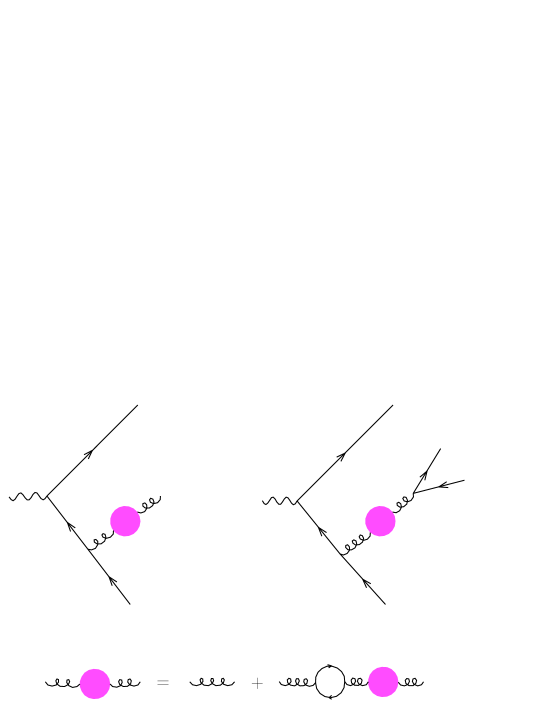
Figure 1: Dominant diagrams for $e^{+}e^{-}$ into jets in the large $n_{f}$ limit.

Notice that there are two types of contribution, one with three partons in the final state and one with four. When taking the square of the amplitude with four final state partons the fermions coming from the gluon splitting should not interfere with those coming from the photon vertex in order to give a dominant term in the large $n_{f}$ limit.

We will now discuss what we expect for the result of the calculation of jet shape variables. The aim of this discussion is simply to give the flavour of how the exact calculation, which will be presented in the following section, works. All details of the infrared cancelation will be dealt with in the next section.

In some appropriate renormalization scheme the inclusion of all vacuum bubbles will amount to the replacement

$$\alpha_{\scriptscriptstyle S}\;\mbox{$\rightarrow$}\;{\alpha_{\scriptscriptstyle S}\over 1+\alpha_{\scriptscriptstyle S}b_{0}\log(-k^{2}/\mu^{2})}$$ (2.1)

where

$$b_{0}=-{T_{R}\over 3\pi}\,,$$ (2.2)

and $T_{R}=n_{f}/2$. The contribution of the graphs with three partons in the final state will be simply given by the Born cross section, with the replacement of eq. (2.1) at $k^{2}=0$. In this limit our expression vanishes, which is to say, we have no virtual graphs after we have resummed the whole perturbative expansion. It does not vanish, however, order by order in perturbation theory, but has instead an expansion with infrared divergent coefficients. In the next section we will show that these divergences are canceled order by order in perturbation theory by the real term. For the sake of the present illustrative discussion, we will instead accept the fact that it vanishes, and concentrate on the finite remainder coming from the real process.

For the corresponding real process, the amplitude will in general have the form

$$A(k^{2},\phi)\;d\phi{d\,k^{2}\over k^{2}}\left|{\alpha_{\scriptscriptstyle S}\over 1+\alpha_{\scriptscriptstyle S}\,b_{0}\left(\log{k^{2}\over\mu^{2}}+i\pi\right)}\right|^{2}$$ (2.3)

where $\phi$ represent here the whole of phase space, except for the virtuality of the gluon, $k^{2}$. In this expression we have factored out the infrared divergent term $dk^{2}/k^{2}$, so that $A(k^{2},\phi)$ is in fact regular for $k^{2}\mbox{$\rightarrow$}0$. Observe that since $k^{2}$ is positive, the logarithm in the running coupling acquires an imaginary part. Let us now suppose that we are computing some infrared safe shape variable $S(k^{2},\phi)$. Infrared safety implies that in the limit of small $k^{2}$ $S(k^{2},\phi)$ goes continuously to its three–body form, so that the cancelation between real and virtual infrared divergences takes place. We define

$$G(k^{2})=\int\;A(k^{2},\phi)\;S(k^{2},\phi)\;d\,\phi\,.$$ (2.4)

The value of $S$ will be given by

$$S=\int{d\,k^{2}\over k^{2}}\;G(k^{2})\;\left|{\alpha_{\scriptscriptstyle S}\over 1+\alpha_{\scriptscriptstyle S}\,b_{0}\left(\log{k^{2}\over\mu^{2}}+i\pi\right)}\right|^{2}$$ (2.5)

which we rewrite as

$$S = \int{d\,k^{2}\over k^{2}}\;[G(k^{2})-G(0)]\;{\alpha_{\scriptscriptstyle S}^{2}\over\left(1+\alpha_{\scriptscriptstyle S}\,b_{0}\log{k^{2}\over\mu^{2}}\right)^{2}+\alpha_{\scriptscriptstyle S}^{2}\pi^{2}b_{0}^{2}}$$ (2.6)

$$+G(0)\int{d\,k^{2}\over k^{2}}\;{\alpha_{\scriptscriptstyle S}^{2}\over\left(1+\alpha_{\scriptscriptstyle S}\,b_{0}\log{k^{2}\over\mu^{2}}\right)^{2}+\alpha_{\scriptscriptstyle S}^{2}\pi^{2}b_{0}^{2}}\,.$$

For the integral in the second term we get

$$G(0)\int{d\,k^{2}\over k^{2}}\;{\alpha_{\scriptscriptstyle S}^{2}\over\left(1+\alpha_{\scriptscriptstyle S}\,b_{0}\log{k^{2}\over\mu^{2}}\right)^{2}+\alpha_{\scriptscriptstyle S}^{2}\pi^{2}b_{0}^{2}}$$

$$={G(0)\over b_{0}^{2}\pi}\left[\arctan\left({1+\alpha_{\scriptscriptstyle S}b_{0}\log{Q^{2}\over\mu^{2}}\over\alpha_{\scriptscriptstyle S}b_{0}\pi}\right)-\arctan\left({1+\alpha_{\scriptscriptstyle S}b_{0}\log{\lambda^{2}\over\mu^{2}}\over\alpha_{\scriptscriptstyle S}b_{0}\pi}\right)\right]$$

$$=-{G(0)\over b_{0}^{2}\pi}\left[\arctan\left({\alpha_{\scriptscriptstyle S}b_{0}\pi\over 1+\alpha_{\scriptscriptstyle S}b_{0}\log{Q^{2}\over\mu^{2}}}\right)-\arctan\left({\alpha_{\scriptscriptstyle S}b_{0}\pi\over 1+\alpha_{\scriptscriptstyle S}b_{0}\log{\lambda^{2}\over\mu^{2}}}\right)\right]$$ (2.7)

where $\lambda$ is an infrared cutoff. There is a subtlety in the second step, where we use the identity $\arctan(x)=\pm\pi/2-\arctan(1/x)$, in which the $\pi/2$ takes the same sign as $x$. Thus our substitution is only correct when the arguments of both arctangents have the same sign. This condition is violated if $b_{0}$ is positive, and it might appear that we have neglected a term proportional to $\pi,$ with no coupling in front. However, we should remember that we are computing a perturbative expansion, and that our algebraic manipulations should always be interpreted as an order by order expansion in $\alpha_{\scriptscriptstyle S}$. We should therefore always be reasoning by assuming that terms with factors of $\alpha_{\scriptscriptstyle S}$ are small, even if multiplied by infrared or ultraviolet divergent coefficients. In this sense eq. (2.7) is correct for either sign of $b_{0}$.

The infrared divergent term we obtain cancels against the virtual diagram. The cancelation is explicitly shown in the next section. Here we just assume that it will take place. In the present context, the real infrared divergent term vanishes in the same sense in which the virtual term was vanishing. We see therefore that the only place where we can obtain an infrared renormalon is the first term of eq. (2.6). Let us assume that $G(k^{2})-G(0)\propto k^{p}$ for small $k,$ and consider the integral

$$I_{p}(Q^{2}) = \int_{0}^{Q^{2}}{dk^{2}\over k^{2}}\;\left({k\over Q}\right)^{p}\;{\alpha_{\scriptscriptstyle S}^{2}\over\left(1+\alpha_{\scriptscriptstyle S}\,b_{0}\log{k^{2}\over\mu^{2}}\right)^{2}+\alpha_{\scriptscriptstyle S}^{2}\pi^{2}b_{0}^{2}}$$ (2.8)

$$= \int_{0}^{\infty}dz\,e^{-pz/2}{\alpha_{\scriptscriptstyle S}^{2}\over\left(1+\alpha_{\scriptscriptstyle S}b_{0}\log{Q^{2}\over\mu^{2}}-\alpha_{\scriptscriptstyle S}b_{0}z\right)^{2}+(\alpha_{\scriptscriptstyle S}b_{0}\pi)^{2}}$$

$$= {1\over b_{0}\pi}\mathop{\rm Im}\left[\int_{0}^{\infty}dz\,e^{-pz/2}{\alpha_{\scriptscriptstyle S}\over 1+\alpha_{\scriptscriptstyle S}b_{0}\log{Q^{2}\over\mu^{2}}-\alpha_{\scriptscriptstyle S}b_{0}z-i\alpha_{\scriptscriptstyle S}b_{0}\pi}\right]$$

$$= {1\over b_{0}\pi}\mathop{\rm Im}\left[\int_{z_{0}}^{z_{0}+\infty}dz^{\prime}\,e^{-p(z^{\prime}-z_{0})/2}{\alpha_{\scriptscriptstyle S}\over 1-\alpha_{\scriptscriptstyle S}b_{0}z^{\prime}}\right]\,,$$

where $z=\log{Q^{2}\over k^{2}}$, $z^{\prime}=z+z_{0}$ and $z_{0}=i\pi-\log{Q^{2}\over\mu^{2}}$. This becomes

$$I_{p}(Q^{2}) = -{1\over b_{0}\pi}\mathop{\rm Im}\left[\int_{0}^{z_{0}}dz^{\prime}\,e^{-p(z^{\prime}-z_{0})/2}{\alpha_{\scriptscriptstyle S}\over 1-\alpha_{\scriptscriptstyle S}b_{0}z^{\prime}}\right]$$ (2.9)

$$+{1\over b_{0}\pi}\mathop{\rm Im}\left[\int_{0}^{\infty}dz^{\prime}\,e^{-p(z^{\prime}-z_{0})/2}{\alpha_{\scriptscriptstyle S}\over 1-\alpha_{\scriptscriptstyle S}b_{0}z^{\prime}-i\epsilon}\right]$$

and the first term is analytic in $\alpha_{\scriptscriptstyle S}$. Rescaling $z^{\prime}$ we finally get

$$I_{p}(Q^{2}) = -{1\over b_{0}\pi}\mathop{\rm Im}\left[\int_{0}^{z_{0}}dz^{\prime}e^{-p(z^{\prime}-z_{0})/2}{\alpha_{\scriptscriptstyle S}\over 1-\alpha_{\scriptscriptstyle S}b_{0}z^{\prime}}\right]$$ (2.10)

$$+{1\over b_{0}^{2}\,\pi}\mathop{\rm Im}\left[e^{i\,p\,\pi/2}\left({\mu\over Q}\right)^{p}\int_{0}^{\infty}dz{\exp(-z/\alpha_{\scriptscriptstyle S})\over{p\over 2b_{0}}-z-i\epsilon}\right]\,.$$

The first term is analytic, while the second term has an infrared renormalon located at $p/(2b_{0})$, which corresponds to a power correction of the order of $1/Q^{p}$. Observe that for positive $b_{0}$ we have found a definite prescription to bypass the IR pole. However, this is not to be trusted, since for positive $b_{0}$ we should interpret our results only as a power expansion in $\alpha_{\scriptscriptstyle S}$, as discussed earlier.

In case the behaviour of $G(k^{2})-G(0)$ is of the type $k^{p}\log^{n}(k/Q)$ instead of a simple power, it is easy to convince oneself that the $1/Q^{p}$ correction will be enhanced by $n$ inverse powers of $\alpha_{\scriptscriptstyle S}$. In fact, the inclusion of powers of $\log(k/Q)$ can be achieved from formula (2.8) by taking derivatives with respect to $p$. Thus, since the large order behaviour of the expansion of $I_{p}$ has the form

$$\propto\Gamma(n+1)\left({2b_{0}\alpha_{\scriptscriptstyle S}\over p}\right)^{n+1},$$ (2.11)

taking a derivative with respect to $p$ we get the leading behaviour

$$\propto{1\over p}\Gamma(n+2)\left({2b_{0}\alpha_{\scriptscriptstyle S}\over p}\right)^{n+1}={1\over 2b_{0}\alpha_{\scriptscriptstyle S}}\Gamma(n^{\prime}+1)\left({2b_{0}\alpha_{\scriptscriptstyle S}\over p}\right)^{n^{\prime}+1}$$ (2.12)

with $n^{\prime}=n+1$, which corresponds to a $1/\alpha_{\scriptscriptstyle S}$ enhancement.

We have therefore found that in our approach the coefficient of the power correction will depend upon the behaviour of $S(\phi,k^{2})$ for small $k^{2}$, which is to say, upon how the definition of the shape variables for 4 partons goes to the 3–parton definition in the collinear limit. This indicates that the coefficient of the power correction cannot be simply factorized in terms of the three–body definition of the shape variable, a fact that we will examine in more details in the following sections.

3. Details of the calculation

We begin with some kinematical preliminaries.

Figure 2: Labeling of external lines for three– and four–parton processes.

Outgoing legs for the three– and four–parton process are given in fig. 2. We will call $p_{i}$ the momenta of the outgoing legs, $E_{i}$ their energies, and the invariants will be defined as

$$Q = \sqrt{\left(\sum p_{i}\right)^{2}}$$

$$s_{ij} = (p_{i}+p_{j})^{2},\quad y_{ij}={s_{ij}\over Q^{2}}$$

$$s_{ijk} = (p_{i}+p_{j}+p_{k})^{2},\quad y_{ijk}={s_{ijk}\over Q^{2}}.$$ (3.1)

For the 4–parton process we have

$$E_{1}={Q^{2}-s_{234}\over 2Q}\,,\quad E_{2}={Q^{2}-s_{134}\over 2Q}\,.$$ (3.2)

In the three-body case these simplify to

$$E_{2}={Q^{2}-s_{13}\over 2Q}\quad\quad E_{1}={Q^{2}-s_{23}\over 2Q}.$$ (3.3)

The maximum value of $s_{34}$ for fixed $s_{134}$ and $s_{234}$ is reached when $\vec{p}_{1}$ and $\vec{p}_{2}$ are parallel and opposite:

$$s_{34}={s_{234}s_{134}\over Q^{2}}.$$ (3.4)

Defining

$$x_{1}={2E_{1}\over Q}=1-y_{234}\,,\quad x_{2}={2E_{2}\over Q}=1-y_{134}$$ (3.5)

we have the constraint

$$s_{34}<Q^{2}(1-x_{1})(1-x_{2})\,.$$ (3.6)

We follow here the calculation of ref. [9], from which many of the following results are taken. We work in $d=4-2\epsilon$ dimensions. The three body cross section is given by the formula

$$d\sigma^{(3)}=H{\alpha_{\scriptscriptstyle S}\over 2\pi}C_{F}\left({4\pi\mu^{2}\over Q^{2}}\right)^{\epsilon}{1\over\Gamma(1-\epsilon)}T(x_{1},x_{2})$$

$$\theta(x_{1}+x_{2}-1)\left((1-x_{1})(1-x_{2})(x_{1}+x_{2}-1)\right)^{-\epsilon}\;\;dx_{1}\;dx_{2}.$$ (3.7)

The constant $H$ is the normalization of the Born 2 body cross section, $\sigma^{(2)}=H$. The four–parton cross section is

$$d\sigma^{(4)}=H{\alpha_{\scriptscriptstyle S}C_{F}\over 2\pi}\left({4\pi\mu^{2}\over Q^{2}}\right)^{\epsilon}{1\over\Gamma(1-\epsilon)}\left((1-x_{1})(1-x_{2})-y_{34}\right)^{-\epsilon}(y_{34}+x_{1}+x_{2}-1)^{-\epsilon}\;$$

$$\theta\left((1-x_{1})(1-x_{2})-y_{34}\right)\;\theta\left(y_{34}+x_{1}+x_{2}-1\right)\;\;dx_{1}\;dx_{2}{\alpha_{\scriptscriptstyle S}T_{R}\over 2\pi}\left({4\pi\mu^{2}\over Q^{2}}\right)^{\epsilon}{1\over\Gamma(1-\epsilon)}$$

$$\left(z(1-z)\right)^{-\epsilon}\;dz\;{1\over N_{\theta}^{\prime}}\sin^{-2\epsilon}\theta^{\prime}d\theta^{\prime}\;\;{dy_{34}\over y_{34}^{1+\epsilon}}\;\;T^{(4)}(x_{1},x_{2},y_{34},z,\theta^{\prime})$$ (3.8)

where

$$T^{(4)}(x_{1},x_{2},y_{34},z,\theta^{\prime}) = T^{(4)}_{\rm coll}(x_{1},x_{2},z,\theta^{\prime})+V(x_{1},x_{2},y_{34},z,\theta^{\prime})$$ (3.9)

$$T^{(4)}_{\rm coll}(x_{1},x_{2},z,\theta^{\prime}) = T(x_{1},x_{2})\;\left({z^{2}+(1-z)^{2}-\epsilon\over 1-\epsilon}\right)$$ (3.10)

$$-R(x_{1},x_{2})\;4z(1-z)\left(2\cos\theta^{\prime}-{1\over 1-\epsilon}\right)$$

$$T(x_{1},x_{2}) = {x_{1}^{2}+x_{2}^{2}\over(1-x_{1})(1-x_{2})}+{\cal O}(\epsilon)$$ (3.11)

$$R(x_{1},x_{2}) = {x_{1}+x_{2}-1\over(1-x_{1})(1-x_{2})}$$ (3.12)

$$\int{1\over N_{\theta}^{\prime}}\sin^{-2\epsilon}\theta^{\prime}d\theta^{\prime} = 1\,.$$ (3.13)

The $V$ term (which can be extracted from ref. [9]) vanishes for $y_{34}\mbox{$\rightarrow$}0$. We have kept the four–parton phase space factorized into a three–parton component, describing the production of a quark, an antiquark and a gluon, and a two–parton term, corresponding to the decay of the virtual gluon into a quark-antiquark pair.

In order to study the infrared renormalon, we must now include all the vacuum polarizations in the three and four–parton processes. First of all, we need a formula for the vacuum polarization in the ${\rm MS}$ scheme. We obtain

$$\Pi_{\mu\nu} = \Pi(k^{2})\;\left(g_{\mu\nu}\;k^{2}-k_{\mu}\,k_{\nu}\right)$$

$$\Pi(k^{2}) = -i{\alpha_{\scriptscriptstyle S}T_{R}\over 3\pi}\;\left({-k^{2}\over\mu^{2}}\right)^{-\epsilon}\;{N(\epsilon)\over\epsilon}$$

$$N(\epsilon) = (4\pi)^{\epsilon}\,\Gamma(1+\epsilon){\Gamma^{2}(1-\epsilon)\over\Gamma(1-2\epsilon)}{1-\epsilon\over(1-{2\over 3}\epsilon)(1-2\epsilon)}\;\stackrel{{\scriptstyle\epsilon\mbox{$\rightarrow$}0}}{{\longrightarrow}}\;1\,.$$ (3.14)

It is now easy to show that insertion of all vacuum blobs into a gluon line amounts to the following replacement

$$\alpha_{\scriptscriptstyle S}\;\mbox{$\rightarrow$}\;{\alpha_{\scriptscriptstyle S}\over 1-\alpha_{\scriptscriptstyle S}b_{0}\left({-k^{2}\over\mu^{2}}\right)^{-\epsilon}{N(\epsilon)\over\epsilon}}\,.$$ (3.15)

The renormalizability of our theory implies that all divergences are removed by a redefinition

$$\alpha_{\scriptscriptstyle S}\mbox{$\rightarrow$}Z\;\alpha_{\rm ren}$$ (3.16)

where in the MS scheme $Z$ is a power expansion in $\alpha_{\rm ren}$, whose coefficients contain only inverse powers of $\epsilon$. After renormalization, our replacement rule will then become

$$\alpha_{\scriptscriptstyle S}\;\mbox{$\rightarrow$}\;{\alpha_{\rm ren}\over Z^{-1}-\alpha_{\rm ren}b_{0}\left({-k^{2}\over\mu^{2}}\right)^{-\epsilon}{N(\epsilon)\over\epsilon}}$$ (3.17)

so that we must have

$$Z^{-1}=1+\alpha_{\rm ren}b_{0}\;{1\over\epsilon}.$$ (3.18)

Therefore, the resummation of all bubbles plus charge renormalization amounts to the replacement

$$\alpha_{\scriptscriptstyle S}\;\mbox{$\rightarrow$}\;{\alpha_{\scriptscriptstyle S}\over 1-\alpha_{\scriptscriptstyle S}b_{0}\left[\left({-k^{2}\over\mu^{2}}\right)^{-\epsilon}N(\epsilon)-1\right]{1\over\epsilon}}.$$ (3.19)

We can now immediately write down the result for the three–parton cross section including the effect of all bubble insertions. In this case, in fact, the momentum flowing through the gluon propagator is exactly zero. Indicating with a tilde the fully resummed cross section we get

$$d\tilde{\sigma}^{(3)}\;=\;d\sigma^{(3)}{1\over 1+\alpha_{\scriptscriptstyle S}b_{0}{1\over\epsilon}}.$$ (3.20)

Observe that in spite of the renormalization procedure we carried out, poles in $\epsilon$ do remain, and they should in fact be interpreted as infrared poles, that will ultimately cancel against analogous contributions in the four–parton cross section.

The case of the four–parton cross section is more involved. In this case one should remember that in the $\alpha_{\scriptscriptstyle S}^{2}$ factor one power of $\alpha_{\scriptscriptstyle S}$ should be complex-conjugated. We then have

$$d\tilde{\sigma}^{(4)} = d\sigma^{(4)}{1\over 1-\alpha_{\scriptscriptstyle S}\,b_{0}\left(y\,e^{i\epsilon\pi}\,N(\epsilon)-1\right){1\over\epsilon}}\;\;{1\over 1-\alpha_{\scriptscriptstyle S}\,b_{0}\left(y\,e^{-i\epsilon\pi}\,N(\epsilon)-1\right){1\over\epsilon}}$$ (3.21)

$$= d\sigma^{(4)}{1\over\left[\left(1+{\alpha_{\scriptscriptstyle S}b_{0}\over\epsilon}\right)\,\cos\epsilon\pi-{\alpha_{\scriptscriptstyle S}b_{0}\over\epsilon}N(\epsilon)\,y\right]^{2}+\left(1+{\alpha_{\scriptscriptstyle S}b_{0}\over\epsilon}\right)^{2}\sin^{2}\epsilon\pi}$$

where we have defined

$$y=\left({s_{34}\over\mu^{2}}\right)^{-\epsilon}.$$ (3.22)

In order to make the infrared cancelation explicit, we will proceed as follows. Let us call $G$ a generic infrared safe jet shape variable. For our purposes, $G$ is characterized by two functions

$$G^{(3)}(x_{1},x_{2}),\quad\quad G^{(4)}(x_{1},x_{2},y_{34},\theta^{\prime},z)$$ (3.23)

and infrared safety will imply that

$$\lim_{y_{34}\mbox{$\rightarrow$}0}G^{(4)}(x_{1},x_{2},y_{34},\theta^{\prime},z)=G^{(3)}(x_{1},x_{2}).$$ (3.24)

We are implicitly assuming that $G$ does not receive contributions from the two–parton final state, and therefore it has a power expansion that starts at order $\alpha_{\scriptscriptstyle S}$, which is the case for all shape variables usually considered in $e^{+}e^{-}$ physics. The value of $G$ in our model will be given by

$$G=\int d\;\tilde{\sigma}^{(3)}G^{(3)}(x_{1},x_{2})+\int d\;\tilde{\sigma}^{(4)}\;G^{(4)}(x_{1},x_{2},y_{34},\theta^{\prime},z).$$ (3.25)

We now rewrite the above expression in the following form

$$G=G_{\rm virt}+G_{4}+G_{V}+G_{\rm coll}$$ (3.26)

with

$$G_{\rm virt} = \int d\;\tilde{\sigma}^{(3)}G^{(3)}(x_{1},x_{2})$$

$$G_{4} = \int d\;\tilde{\sigma}^{(4)}\;\Big{[}G^{(4)}(x_{1},x_{2},y_{34},\theta^{\prime},z)-F(x_{1},x_{2},y_{34})\,G^{(3)}(x_{1},x_{2})\Big{]}$$

$$G_{V} = \int d\;\tilde{\sigma}_{V}^{(4)}\;F(x_{1},x_{2},y_{34})\;G^{(3)}(x_{1},x_{2})$$

$$G_{\rm coll} = \int d\;\tilde{\sigma}_{\rm coll}^{(4)}\;F(x_{1},x_{2},y_{34})\;G^{(3)}(x_{1},x_{2}),$$ (3.27)

and

$$F(x_{1},x_{2},y_{34}) = {((1-x_{1})(1-x_{2})-y_{34})^{\epsilon}\,(y_{34}+x_{1}+x_{2}-1)^{\epsilon}\over((1-x_{1})(1-x_{2}))^{\epsilon}\,(x_{1}+x_{2}-1)^{\epsilon}}\theta(x_{1}+x_{2}-1)$$

$$d\tilde{\sigma}^{(4)} = d\tilde{\sigma}^{(4)}_{V}+d\tilde{\sigma}^{(4)}_{\rm coll}.$$ (3.28)

The separation of $d\sigma^{(4)}$ into the collinear and $V$ term is performed according to eq. (3.9). The $F$ factor is chosen in order to simplify the $y_{34}$ integral in the $G_{\rm coll}$ term. The $G_{4}$ and $G_{V}$ terms are free of infrared singularities, because the integrands vanish for $y_{34}\mbox{$\rightarrow$}0$, so that $\epsilon$ can be safely replaced by 0 in their expressions. In ref. [10] it was shown that after $\theta^{\prime}$ and $z$ integration $G_{V}$ is of order $y_{34}$. In $G_{\rm coll}$, the integration in $z$, $\theta^{\prime}$ and $y_{34}$ can be performed, because $G^{(3)}$ does not depend upon these quantities. The $z$ and $\theta^{\prime}$ integrals are easily done. The $R$ term vanishes after angular integration, and the $z$ integration gives

$$\int dz\,(z(1-z))^{-\epsilon}\;{z^{2}+(1-z)^{2}-\epsilon\over 1-\epsilon}={\Gamma^{2}(1-\epsilon)\over\Gamma(1-2\epsilon)}{2(1-\epsilon)\over(1-2\epsilon)(3-2\epsilon)}={2N(\epsilon)\over 3\,(4\pi)^{\epsilon}\Gamma(1+\epsilon)}\,.$$ (3.29)

Using the identity

$${dy_{34}\over y_{34}^{1+\epsilon}}=-{dy\over\epsilon}\,\left({Q^{2}\over\mu^{2}}\right)^{\epsilon}$$ (3.30)

we compute the $y_{34}$ integral

$$\int_{0}^{(1-x_{1})(1-x_{2})}{dy_{34}\over y_{34}^{1+\epsilon}}{1\over\left[\left(1+{\alpha_{\scriptscriptstyle S}b_{0}\over\epsilon}\right)\,\cos\epsilon\pi-{\alpha_{\scriptscriptstyle S}b_{0}\over\epsilon}N(\epsilon)\,y\right]^{2}+\left(1+{\alpha_{\scriptscriptstyle S}b_{0}\over\epsilon}\right)^{2}\sin^{2}\epsilon\pi}$$

$$={-\left({Q^{2}\over\mu^{2}}\right)^{\epsilon}\over\alpha_{\scriptscriptstyle S}\,b_{0}\,N(\epsilon)\left(1+{\alpha_{\scriptscriptstyle S}b_{0}\over\epsilon}\right)\sin\epsilon\pi}\;\;\left.\arctan{\left(1+{\alpha_{\scriptscriptstyle S}b_{0}\over\epsilon}\right)\sin\epsilon\pi\over\left(1+{\alpha_{\scriptscriptstyle S}b_{0}\over\epsilon}\right)\cos\epsilon\pi-{\alpha_{\scriptscriptstyle S}b_{0}\over\epsilon}\,N(\epsilon)y}\right|^{(1-x_{1})(1-x_{2})}_{0}$$

$$=-{1\over\alpha_{\scriptscriptstyle S}^{2}\,b_{0}^{2}\,\pi}\arctan{\alpha_{\scriptscriptstyle S}\,b_{0}\,\pi\over 1+\alpha_{\scriptscriptstyle S}\,b_{0}\,\left(\log{(1-x_{1})(1-x_{2})Q^{2}\over\mu^{2}}-N^{\prime}(0)\right)}$$

$$+\left({Q^{2}\over\mu^{2}}\right)^{\epsilon}{\epsilon\pi\over\alpha_{\scriptscriptstyle S}\,b_{0}\,N(\epsilon)\left(1+{\alpha_{\scriptscriptstyle S}b_{0}\over\epsilon}\right)\sin\epsilon\pi}$$ (3.31)

where we have set explicitly $\epsilon=0$ in the first term. Using the identity

$${\epsilon\pi\over\sin\epsilon\pi\,\Gamma(1+\epsilon)\Gamma(1-\epsilon)}=1$$ (3.32)

we write our integral as

$$G_{\rm coll}=-\int{\alpha_{\scriptscriptstyle S}C_{F}\over 2\pi}\theta\left(x_{1}+x_{2}-1\right)\;\;dx_{1}\;dx_{2}$$

$$\times{\alpha_{\scriptscriptstyle S}T_{R}\over 3\pi}T(x_{1},x_{2})\;G^{(3)}(x_{1},x_{2}){1\over\alpha_{\scriptscriptstyle S}^{2}\,b_{0}^{2}\,\pi}\arctan{\bar{\alpha}_{\scriptscriptstyle S}\,b_{0}\,\pi\over 1+\bar{\alpha}_{\scriptscriptstyle S}\,b_{0}\,\log{(1-x_{1})(1-x_{2})Q^{2}\over\mu^{2}}}$$

$$+\int H{\alpha_{\scriptscriptstyle S}C_{F}\over 2\pi}\left({4\pi\mu^{2}\over Q^{2}}\right)^{\epsilon}{1\over\Gamma(1-\epsilon)}\theta\left(x_{1}+x_{2}-1\right)[(1-x_{1})(1-x_{2})(x_{1}+x_{2}-1)]^{-\epsilon}$$

$$\times{\alpha_{\scriptscriptstyle S}T_{R}\over 3\pi}{1\over\alpha_{\scriptscriptstyle S}\,b_{0}\,\left(1+{\alpha_{\scriptscriptstyle S}b_{0}\over\epsilon}\right)}T(x_{1},x_{2})\;G^{(3)}(x_{1},x_{2})\;\;dx_{1}\;dx_{2}$$ (3.33)

where we have defined according with ref. [11]

$${1\over\bar{\alpha}_{\scriptscriptstyle S}}={1\over\alpha_{\scriptscriptstyle S}}-N^{\prime}(0).$$ (3.34)

Remembering the identity for $b_{0}$ we see that the second integral in the above equation cancels exactly $G_{\rm virt}$, so that all infrared divergences cancel, and we can write

$$G=G_{4}+G_{V}+G_{S}\,,\quad\quad G_{S}=G_{\rm virt}+G_{\rm coll}\,.$$ (3.35)

The $G_{S}$ term is given by the first term of eq. (3.33), and the $S$ suffix stands for “Sudakov”, since (in some sense) this term comes from the incomplete cancelation between the real and virtual diagrams, induced by the running of $\alpha_{\scriptscriptstyle S}$. It can be written as

$$G_{S}={C_{F}\over 2\pi}\int_{x_{1}+x_{2}<1}\;\;dx_{1}\;dx_{2}\;T(x_{1},x_{2})\;G^{(3)}(x_{1},x_{2}){\arctan(\bar{\alpha}_{\scriptscriptstyle S}(k_{\perp}^{2})\,b_{0}\,\pi)\over b_{0}\,\pi}$$ (3.36)

where

$$k_{\perp}^{2}=(1-x_{1})(1-x_{2})\;Q^{2}\,.$$ (3.37)

4. The Sudakov term

A term of the form of $G_{S}$ appeared first in ref. [5], and was there used to parameterize the $1/Q$ correction to shape variables like the average value of $1-t$, where $t$ is the thrust. In ref. [6] it was argued that the power corrections of the order $1/Q$ factorize in the form of eq. (3.36) for a generic shape variable, as well as for other processes. In our calculation, this term, before the $x_{1},x_{2}$ integration, does not have any renormalon, since it is an analytic function of $\alpha_{\scriptscriptstyle S}$ near the origin. When we integrate over $x_{1},x_{2}$, and approach the singular two–jet region, non–analytic behaviour may arise. This is due to the fact that we are integrating over the $x_{1},x_{2}$ values where

$$1/\bar{\alpha}_{\scriptscriptstyle S}(k_{\perp}^{2})=1+\bar{\alpha}_{\scriptscriptstyle S}b_{0}\log{k_{\perp}^{2}\over\mu^{2}}\;\mbox{$\rightarrow$}\;0\,.$$ (4.1)

Our formula differs from the one of ref. [5] only by the replacement

$$\bar{\alpha}_{\scriptscriptstyle S}(q^{2})\mbox{$\rightarrow$}{1\over b_{0}\pi}\arctan(\bar{\alpha}_{\scriptscriptstyle S}(q^{2})b_{0}\pi)\,.$$ (4.2)

In our case, however, there is really no singularity when we integrate over the Landau pole, since the arctangent is a bounded function. Let us compute the contribution of the $G_{S}$ term to the average value of $1-t$. For a three massless body system, thrust is simply

$$t=\max(x_{1},x_{2},2-x_{1}-x_{2}).$$ (4.3)

The leading contribution to $1-t$ comes from the region where $x_{1}$ and $x_{2}$ are very near 1, so

$$\langle 1-t\rangle_{S} = {C_{F}\over 2\pi}2\int_{x_{1}>x_{2}}dx_{1}dx_{2}\;{2(1-x_{1})\over(1-x_{1})(1-x_{2})}{\arctan(\bar{\alpha}_{\scriptscriptstyle S}(k_{\perp}^{2})b_{0}\pi)\over b_{0}\pi}$$ (4.4)

$$= {2C_{F}\over\pi}\int_{0}^{1}{dy\over\sqrt{y}}\;{\arctan(\bar{\alpha}_{\scriptscriptstyle S}(yQ^{2})b_{0}\pi)\over b_{0}\pi}\,.$$

In order to evidentiate the structure of the infrared renormalon in the above formula, we compute the integral

$$I=\int_{0}^{1}{dy\over y}\;y^{p\over 2}{\arctan(\bar{\alpha}_{\scriptscriptstyle S}(yQ^{2})b_{0}\pi)\over b_{0}\pi}$$ (4.5)

for arbitrary $p>0$. We integrate by parts, and obtain

$$I = {2\arctan(\bar{\alpha}_{\scriptscriptstyle S}(Q)b_{0}\pi)\over p\,b_{0}\,\pi}+{2\over p}\int_{0}^{1}{dy\over y}\,y^{{p\over 2}}{b_{0}\over{1\over\bar{\alpha}_{\scriptscriptstyle S}^{2}(yQ^{2})}+(b_{0}\pi)^{2}}$$ (4.6)

$$= {2\arctan(\bar{\alpha}_{\scriptscriptstyle S}(Q)b_{0}\pi)\over p\,b_{0}\,\pi}+{2b_{0}\over p}\;I_{p}\,.$$

The first term is analytic in $\bar{\alpha}_{\scriptscriptstyle S}$ near the origin, while the second term, given by eq. (2.10) has an infrared renormalon located at $z=p/(2b_{0})$, which corresponds to a $1/Q^{p}$ power correction. For the case of $\langle 1-t\rangle$ we found therefore a $1/Q$ correction.

5. The four–parton integral

The terms $G_{4}$ and $G_{V}$ cannot easily be done analytically, because they depend in an intricate way on the four–parton phase space. Observe that

$$G_{4}+G_{V} = \int\Big{[}\;d\,\tilde{\sigma}^{(4)}\;G^{(4)}(x_{1},x_{2},y_{34},\theta^{\prime},z)-\theta(x_{1}+x_{2}-1)\;d\,\tilde{\sigma}^{(4)}_{\rm coll}\,G^{(3)}(x_{1},x_{2})\;\Big{]}$$ (5.1)

$$= \int dy\;G_{4V}(y){\bar{\alpha}_{\scriptscriptstyle S}^{2}\over\left(1+\bar{\alpha}_{\scriptscriptstyle S}b_{0}\log{yQ^{2}\over\mu^{2}}\right)^{2}+(\bar{\alpha}_{\scriptscriptstyle S}b_{0}\pi)^{2}}\,,$$

where we have defined

$$G_{4V}(y) = {1\over\bar{\alpha}_{\scriptscriptstyle S}^{2}}\int\delta(y-y_{34})\Big{[}\;d\,\sigma^{(4)}\;G^{(4)}(x_{1},x_{2},y_{34},\theta^{\prime},z)$$ (5.2)

$$-\theta(x_{1}+x_{2}-1)\;d\,\sigma^{(4)}_{\rm coll}\,G^{(3)}(x_{1},x_{2})\;\Big{]}\,.$$

It is clear that the small $y$ behaviour of $G_{4V}(y)$ controls the power correction due to the IR renormalon. In particular, if

$$G_{4V}(y)\stackrel{{\scriptstyle y\mbox{$\rightarrow$}0}}{{\longrightarrow}}A\;{y^{p/2}\over y}$$ (5.3)

the position of the renormalon will be at $p/(2b_{0})$, corresponding to a power correction $1/Q^{p}$.

We computed $G_{4V}$ numerically for $y=10^{-j}$, $j=1,\ldots 6$, for the following shape variables: $\langle 1-t\rangle$, $\langle\theta(0.8-t)\rangle$, $\langle m_{H}^{2}\rangle$, where $m_{H}^{2}$ is the heavy jet mass-squared according to the thrust definition, $\langle\theta(m_{H}^{2}-0.1)\rangle$, $\langle\theta(o-0.1)\rangle$, $\langle\theta(c-0.2)\rangle$, and for the weighted average of the energy-energy correlation away from the back-to-back region

$$EEC_{\rm cut}=\int_{-0.5}^{0.5}EEC(\cos\theta)\;\sin^{2}\theta\;d\cos\theta.$$ (5.4)

For the exact definition of these quantities, see ref. [12]. The results are given in table 1. For each value $y=10^{-j}$, we also give the power $p$ that is obtained by fitting $G_{4V}(y)$ in the two points $10^{-(j-1)}$ and $10^{-j}$ with a function proportional to $y^{p/2}/y$.

$y$	$10^{-1}$	$10^{-2}$	$10^{-3}$	$10^{-4}$	$10^{-5}$	$10^{-6}$
$\langle 1-t\rangle$	.2365(11)	-2.146(7)	-12.21(3)	-46.34(15)	-159.2(6)	-522(3)
$p$	*	*	.490(4)	.842(4)	.928(5)	.969(6)
$t<0.8$	.611(3)	-.566(13)	1.435(10)	2.341(10)	2.469(10)	2.477(10)
$p$	*	*	*	1.575(7)	1.954(5)	1.997(5)
$\langle m_{H}^{2}\rangle$	.0437(11)	-4.595(12)	-25.31(7)	-109.6(4)	-435.8(19)	-1639(9)
$p$	*	*	.518(3)	.727(4)	.801(5)	.849(6)
$m^{2}_{H}>0.1$	.384(2)	-30.22(7)	-62.8(3)	-66.0(5)	-13.60(15)	-.035(10)
$p$	*	*	1.365(4)	1.956(7)	3.372(11)	7.2(2)
$o>0.1$	.252(4)	-119.6(3)	-1856(5)	-5250(30)	-14610(140)	-44600(800)
$p$	*	*	-.381(3)	1.098(5)	1.110(9)	1.031(17)
$c>0.2$	.934(3)	-21.11(11)	-110.5(10)	-129(3)	-145(11)	-150(30)
$p$	*	*	.563(9)	1.86(2)	1.90(7)	2.0(2)
$EEC_{\rm cut}$	.4150(18)	-2.12(2)	-13.9(2)	-51.8(13)	-180(8)	-630(40)
$p$	*	*	.371(16)	.85(3)	.92(4)	.92(7)

Table 1: Results for $G_{4V}(y)$ for various shape variables, for $y=10^{-1},\ldots 10^{-6}$. The line marked $p$, in the column corresponding to $y=10^{-k}$, is the exponent one would obtain from the above table by fitting the pair of numbers on the line above, corresponding to $y=10^{-k+1}$ and $y=10^{-k}$ with the form $y^{p/2}/y$.

As anticipated in the previous section, we can see from the table that the four–parton contribution can give $1/Q$ power suppressed corrections to quantities like the average value of $1-t$.

It is easy to identify regions of integration that give such type of contributions. Consider for example the region

$$\sqrt{y_{34}}<(1-x_{1})<\sqrt{y_{34}}(1+\eta)\,\quad\quad\sqrt{y_{34}}<(1-x_{2})<\sqrt{y_{34}}(1+\eta)$$ (5.5)

for $\eta\ll 1$ and independent of $y_{34}$. In this configuration, $1-t$ is always of order $\sqrt{y_{34}}$. For small $y_{34}$ the emitted gluon is soft, so that the amplitude factorizes in terms of the three body amplitude in the soft limit, and a term depending upon the orientation of partons 3 and 4. The three body amplitude gives an integral of the form

$$\int_{\sqrt{y_{34}}}^{\sqrt{y_{34}}(1+\eta)}{d(1-x_{1})\over 1-x_{1}}{d(1-x_{2})\over 1-x_{2}}=\eta^{2}+{\cal O}(\eta^{3}),$$ (5.6)

independent of $y_{34}$. Next, we have to weight the amplitude with $1-t$, which is of order $\sqrt{y_{34}}$, and integrate in $d\,y_{34}/y_{34}$. This corresponds to $G_{4V}\propto\sqrt{y_{34}}/y_{34}$, which, as we have seen, yields a $1/Q$ correction.

One may wonder whether one may still recover a factorized form, similar to the term $G_{S}$, by a suitable redefinition of the effective coupling. Looking at the quantity $\langle m_{H}^{2}\rangle$ we see that this is not the case. In fact, the invariant mass of the heavy jet is equivalent at the 3–parton level to thrust, namely we have $1-t=m_{H}^{2}/Q^{2}$. This identity is no longer valid at the 4–parton level. For example, in the soft configuration we have just considered, where partons 1 and 2 are back–to–back, and so are partons 3 and 4, it is a simple exercise to show that the relation is instead $1-t=2m_{H}^{2}/Q^{2}$. Therefore, any three–body factorization formula would fail in this simple case. Shape variables that are identical at the 3–parton level, but differ at the 4–parton level, have different coefficients for the leading power correction.

Let us now focus on shape variables that depend upon final state configurations that are far from the two jet region, for which the Sudakov term does not provide a leading $1/Q$ power correction. For some of these variables, e.g. $\langle\theta(0.8-t)\rangle$, $\langle\theta(m_{H}^{2}-0.1)\rangle$, $\langle\theta(c-0.2)\rangle$, we see no evidence for power corrections of the form $1/Q$, but instead we find a $1/Q^{2}$ correction (in the case of $\langle\theta(m_{H}^{2}-0.1)\rangle$, the $1/Q^{2}$ term has a rather small coefficient, so this behaviour does not become apparent until $y\;\raisebox{-1.72218pt}{\hbox to0.0pt{$\sim$\hss}}\raisebox{1.72218pt}{$<$}\;10^{-8},$ where $G_{4V}(y)$ becomes constant at +1.43, indicating $p=2$). For $\langle\theta(o-0.1)\rangle$ we instead observe a $1/Q$ type of correction. A leading $1/Q$ correction is also observed for $EEC_{\rm cut}$, in spite of the cut that avoids the back–to–back region. As we will see shortly, this is due to the fact that $EEC$ receives contributions from configurations near the two jet region also for angles far away from the back–to–back configuration.

These findings can be easily justified by examining the singular integration region for various quantities. First of all we will consider thrust. Let us look at parton configurations near the collinear limit. By kinematical reasoning one can convince oneself that the thrust axis is either along parton 1, parton 2, or along the sum of partons 3 and 4, and the thrust is given by $x_{1}$, $x_{2}$, or $(2-x_{1}-x_{2})-2y_{34}/t+{\cal{O}}(y_{34}^{2})$ respectively. In all cases, it differs from the thrust of the corresponding configuration with $y_{34}=0$ by terms of the order of $y_{34}$ or less. This behaviour gives rise to a $1/Q^{2}$ power correction. In the case of oblateness, we can instead identify a region where a $\sqrt{y_{34}}$ behaviour arises, leading to a $1/Q$ power correction. One such configuration is depicted in Figure 3.

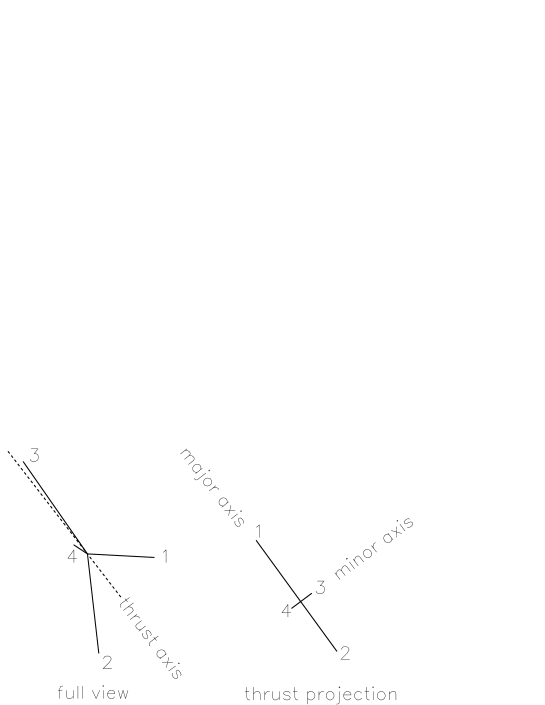
Figure 3: Oblateness in the collinear limit.

One projects the event onto the plane orthogonal to the thrust axis, and then oblateness is defined as the difference between the major and minor axis. For the particular configuration shown in the figure, oblateness is just the difference between the distance 1–2 (called $f$–major) and the distance 3–4 (called $f$–minor) in the projected event. It is easy to convince oneself that the 3–4 distance is proportional to $\sqrt{y_{34}}$. In the limit of $y_{34}\mbox{$\rightarrow$}0$ oblateness behaves therefore like $\sqrt{y_{34}}$, which generates a $1/Q$ correction.

The $1/Q$ correction in the case of the energy–energy correlation has instead a very different origin. One such correction arises from the Sudakov term. In the 3–body configuration, when parton 3 is soft, the Sudakov term for the energy–energy correlation is

$$\sin^{2}\theta\;EEC(\cos\theta)=8\,{C_{F}\over 2\pi}{1\over\sin\theta}\int_{0}^{{1\over 2}Q\sin\theta}{dk_{\perp}\over Q}\;{\arctan(\bar{\alpha}_{\scriptscriptstyle S}(k_{\perp}^{2})b_{0}\pi)\over b_{0}\pi}.$$ (5.7)

The integral over $k_{\perp}$ generates a $1/Q$ correction. Other contributions come from the $G_{4V}$ term. Consider some weighted average of the energy–energy correlation, with a weight $f(\theta)$ in an angular interval that does not include the back–to–back region. Then, for example, the contributions coming from partons 1 and 3 would be

$$\int d\sigma_{3}\;f(\theta)\;E_{1}\,E_{3}\,.$$ (5.8)

If parton 3 (the gluon) splits into a quark–antiquark pair, carrying fractions $z$ and $1-z$ of parton 3’s momentum, and having an opening angle $\omega$. Also assume for simplicity that the splitting takes place in the 1–3 plane. The contribution in the collinear limit is then

$$\int d\sigma_{4}\;E_{1}\,E_{3}\;\left(f(\theta+z\omega)(1-z)+f(\theta-(1-z)\omega)z\right)$$

$$\approx\int d\sigma_{4}\;E_{1}\,E_{3}\;\left(f(\theta)+{1\over 2}\;f^{\prime\prime}(\theta)\omega^{2}\,z(1-z)\right)$$

$$=\int d\sigma_{4}\;E_{1}\,E_{3}\;\left(f(\theta)+{1\over 2}\;f^{\prime\prime}(\theta)s_{34}/E_{3}^{2}\right),$$ (5.9)

which seems to give rise to a $1/Q^{2}$ power correction. This is in fact not the case, since we integrate over the region where $E_{3}$ becomes small. In this region the cross section behaves as $dE_{3}/E_{3}$, so the $E_{3}$ integral in eq. (5.9) yields

$$\int_{\sqrt{s_{34}}}{dE_{3}\over E_{3}^{2}}\propto{1\over\sqrt{s_{34}}}\,,$$ (5.10)

and we see that in this way a $1/Q$ power correction does arise. Therefore, the energy–energy correlation receives $1/Q$ power corrections for all values of the angle, coming from the region near the two–jet limit. It might appear that if we set $f(\theta)={}$constant, this $1/Q$ correction would be zero. However there would still remain $\theta$-function weights defining the edges of the integration region, which would give equivalent $1/Q$ terms.

Unlike the case of oblateness, we see that for the EEC the correction arises because the kinematic region near the two–jet configuration contributes for all values of the angle. All other commonly considered shape variables depend instead upon the three jet region for intermediate values of the shape parameter.

6. Higher order terms

We have seen from the previous section that, except for special cases like oblateness, $1/Q$ corrections arise from configurations with a soft gluon emission, where the gluon virtuality is of the order of its energy, followed by the decay of the virtual gluon into massless partons. This process cannot occur away from the two jet region at leading $n_{f}$, but it can certainly arise at subleading $n_{f}$. We may imagine adding to a three–jet, $q\bar{q}g$ configuration a soft, off–shell gluon (i.e. with energy of the same order as its virtuality) decaying into a massless parton pair. It is difficult to imagine any shape variable that will not receive $1/Q$ corrections from this kind of process. In fact, shape variables are typically linear in the parton momenta, as dictated by the requirement of insensitivity to collinear splitting. The production of a soft, off–shell gluon reduces linearly the energy available to all the other partons, which in general may affect the shape variable linearly in the gluon energy. Since the cross section for soft gluon emission has the characteristic behaviour $dE_{g}/E_{g}$, and the emission coupling will be evaluated at the virtuality of the gluon (assumed to be of the same order as $E_{g}$) it follows that $1/Q$ corrections are present. We have not, of course, rigorously proven this fact. Needless to say, if shape variables that never develop $1/Q$ corrections were found, their importance for the determination of $\alpha_{\scriptscriptstyle S}$ would be enormous.

Let us therefore assume, for a moment, the pessimistic (and perhaps realistic) view that shape variables always develop a $1/Q$ correction at some order in perturbation theory. Let us consider, for example, thrust with a cut $t<0.8$, so that we are always in the three jet region. According to the above argument an extra soft gluon emission will generate a correction of order $1/Q$. It seems plausible however that the hard real emission contributes a factor of $\alpha_{\scriptscriptstyle S}(Q^{2})$, such that the overall correction is of the order of $\alpha_{\scriptscriptstyle S}(Q)/Q$. This would again be a very important fact. It would tell us that some shape variables are indeed better than others, in the sense that their $1/Q$ power correction carries an extra $\alpha_{\scriptscriptstyle S}(Q)$ suppression.

It may also be possible that the $1/Q$ suppression will turn out to be enhanced by a power of $\log(Q/\Lambda)$, which would compensate the $\alpha_{\scriptscriptstyle S}$ suppression. This could be produced, for example, by a 5–parton term that behaved as $\sqrt{y_{45}}\log y_{45}$ when particles 4 and 5 become collinear. Whether these logarithmic enhancements are present or not is a matter that ought to be clarified with further studies. In the present work, we simply remark that it is conceivable that one may find shape variables in which the enhancement is not present, and that therefore do have a $\alpha_{\scriptscriptstyle S}$ suppression of the $1/Q$ power corrections.

7. Conclusions

In the present work, we have proven that even in the simple model of QCD at large $n_{f}$, shape variables in $e^{+}e^{-}$ annihilation show remarkably different properties with regard to power corrections originating from infrared renormalons. In particular, we have shown that in the large $n_{f}$ limit, variables like $\langle 1-t\rangle$, $\langle m_{H}^{2}\rangle$, and the $EEC$ for any value of the angle, develop a $1/Q$ correction, while thrust and the $c$ parameter do not develop any $1/Q$ correction in the region where the two jet configuration does not contribute. Another remarkable result is that oblateness develops a $1/Q$ correction even away from the two jet region.

We compare our findings with the results of refs. [5] and [6]. We recover a correction term with the factorized form proposed there, but we also find an extra correction that spoils factorization, since it specifically depends upon the 4–parton definition of the shape variable. Thus, two shape variables that have the same 3–body expression, but differ at the 4–body level, will have different power corrections. The discrepancy with the authors of ref. [5] can be tracked back to the fact that they assume to some extent the validity of the perturbative expansion even when the scale of $\alpha_{\scriptscriptstyle S}$ is very low, a fact that does not take place in our calculation in the leading $n_{f}$ limit.

We argue that even shape variables that do not develop a $1/Q$ correction at the leading large $n_{f}$ level, may develop one at subleading level, and therefore in the full QCD. We conjecture that the leading power correction to shape variables will have in general the form $\alpha^{n}_{\rm S}(Q)/Q$, and one may classify shape variables according to the value of $n$. It may therefore be possible to find a class of shape variables with leading power correction of the form $\alpha_{\scriptscriptstyle S}(Q)/Q$. With these shape variables, the influence of non–perturbative effects upon the determination of $\alpha_{\scriptscriptstyle S}$ would be truly negligible at LEP energies.

References

[1]
S. Bethke, “Experimental Results on QCD and Jets at LEP and SLC”,
PITHA-94-29, Talk given at Tennessee International Symposium on Radiative
Corrections: Status and Outlook, Gatlinburg, TN, 27 June - 1 July 1994.
[2]
B.R. Webber, “QCD and Jet Physics”, proceedings of the XXVII
International Conference on HIgh Energy Physics,
Glasgow, UK, 20-27 July 1994, Editors P.J. Bussey and I.G. Knowles,
Institute of Physics Publishing, Bristol and Philadelphia.
[3]
A.H. Mueller, Proceedings of the Conference “QCD 20 years later”,
Aachen, June 9-13, 1992, editors P.M. Zerwas and H.A. Kastrup,
World Scientific Publishing Co. .
[4]
B.R. Webber, Phys. Lett.B339 (94) 148.
[5]
Yu.L. Dokshitzer and B.R. Webber, Cavendish-HEP-95/2, LU TP 95-8,
hep-ph/9504219.
[6]
R. Akhoury and V.I. Zakharov, SPhT Saclay T95/043, UM-TH-95-12.
[7]
A.V. Manohar and M.B. Wise, Phys. Lett.B344 (95) 407.
[8]
C.N. Lovett-Turner and C.J. Maxwell, Nucl. Phys.B432 (94) 147;
C.N. Lovett-Turner and C.J. Maxwell, Preprint DTP/95/36,
hep-ph/9505224.
[9]
R.K. Ellis, D.A. Ross and A.E. Terrano, Nucl. Phys.B178 (81) 421.
[10]
M.H. Seymour, Nucl. Phys.B436 (95) 163.
[11]
S. Catani, G. Marchesini and B.R. Webber, Nucl. Phys.B349 (91) 635.
[12]
Z. Kunszt and P. Nason, “QCD at LEP”, from “ Physics
at LEP 1”, edited by G. Altarelli, R. Kleiss and C. Verzagnassi,
CERN 89-08, Vol. 1, 21 Sept. 1989.