KUNS-1350

HE(TH) 95/10

hep-ph/9506294

Chiral Symmetry, Heavy Quark Symmetry

and

Bound States

Yuhsuke Yoshida

Department of Physics, Kyoto University
Kyoto 606-01, Japan

January 5, 1995

Abstract

I investigate the bound state problems of lowest-lying mesons and heavy mesons. Chiral symmetry is essential when one consider lowest-lying mesons. Heavy quark symmetry plays an central role in considering the semi-leptonic form factors of heavy mesons. Various properties based on the symmetries are revealed using Bethe-Salpeter equations.

1 Introductions

Chiral Symmetry

The masses of $u$ and $d$ quarks are sufficiently smaller than the typical interaction scale $\Lambda_{\rm QCD}$ of the strong interaction. It is a good picture that the system possesses the $SU(2)_{L}\times SU(2)_{R}$ chiral symmetry.[9, 10]

There are two important low-energy phenomena in the system. First one is that quarks form bound states. In the first part of this review, we consider lowest-lying mesons using Bethe-Salpeter equations. Second one is the dynamical breaking of the chiral symmetry. The physical manifestation of the chiral symmetry is the presence of the Nambu-Goldstone bosons such as pions.[9, 10] The actual pion, even though it has non-zero mass, is recognized to be the Nambu-Goldstone boson of the chiral symmetry. The pion is a pseudoscalar bound state of quarks, and is described by a homogeneous Bethe-Salpeter equation. The Bethe-Salpeter equation of the pion is solved in the chiral limit with the help of the axial Ward-Takahashi identity.[6, 19]

The simplest order parameter of the chiral symmetry breaking is the vacuum expectation value of the quark bilinear $\langle 0|\overline{q}q|0\rangle$ which is calculated using the Schwinger-Dyson equation in the improved ladder approximation. The vacuum expectation value depends on a renormalization point. The low-energy parameter $L_{10}$ which is introduced by Gasser-Leutwyler[13], or so-called $S$ parameter[15] in QCD, is best and well-defined order parameter of the chiral symmetry breaking, because it is a finite quantity which is free from ultraviolet divergences. We have the value $S=0.43\sim 0.48$ in the improved ladder exact approximation.[14] This means the dynamical symmetry breaking of the symmetry in that approximation.

The Nambu-Goldstone bosons, as well as lowest-lying mesons, control many physical processes under low energy theorems. The difference of the vector and axial-vector two-point functions, which we call ‘V-A’ two-point function, is exactly saturated by the contribution of the massless pion and its derivative, the QCD $S$ parameter, is dominated by the contributions of lowest-lying mesons such as $\rho$ and $a_{1}$ mesons in the low-energy limit.

Heavy Quark Symmetry

Recently, there has been many investigations on the $B$ meson in order to define or verify the detailed structure of the Standard Model and to revile new physics beyond it. When we extract the absolute value of one component of the Cabbibo-Kobayashi-Maskawa (CKM) flavor mixing matrix $|V_{\rm cb}|$,[25, 26] we use the exclusive semi-leptonic decay process of the $B$ meson $B\!\rightarrow\!D^{(*)}l\overline{\nu}$. This decay process is intensively studied by using the heavy quark effective theory. When we consider mesons containing a heavy quark (such as the $b$ or $c$ quark), a new approximate symmetry called heavy quark spin-flavor symmetry appears.[27, 28]

According to the heavy quark effective theory[29, 34], when the heavy quark mass goes to infinity, every form factor of the semi-leptonic $B$ decay is expressed in terms of a single universal function, the Isgur-Wise function $\xi(t)$. It is known that the Isgur-Wise function is normalized to unity at the kinematical end point $\xi(1)=1$. The notion of universal form factor was discussed in Ref.[35] first. The normalization of the semi-leptonic decay form factors at the kinematical end point was first suggested in Ref.[36]. The inclusion of $1/M_{Q}$ corrections is studied in Refs.[34, 63].

The measurement of the semi-leptonic decay $B\!\rightarrow\!D^{(*)}l\overline{\nu}$ enables us to know its differential decay rate which is proportional to $|V_{\rm cb}|^{2}$ and the relevant form factors squared. From the condition $\xi(1)=1$ the differential decay rate divided by some phase volume is nothing but $|V_{\rm cb}|^{2}$ at the kinematical end point. Then, we can extract $|V_{\rm cb}|$ without knowing the dynamics of the strong interaction in the $B$ meson.

However, the kinematical end point is actually the end point in phase space, and the volume of the phase space is almost zero. The event is very rare, and we have relatively large statistical error. Moreover, there is a serious difficulty arising from the successive decay $D^{*}\!\rightarrow\!D$ with soft pion emitted. This increases the systematic error. In order to extract $|V_{\rm cb}|$ we have to know the Isgur-Wise function away from the kinematical end point so that we extrapolate the experimental data to the kinematical end point. For this purpose we have to solve the QCD dynamics in the $B$ mesons.

Under these circumstances we deal with this problem by using the Bethe-Salpeter equation, and we calculate the Isgur-Wise function $\xi(t)$ and extract $|V_{\rm cb}|$. To say more concretely we solve the pseudoscalar BS equation for the heavy-light quark system in the three approximations; i) constant quark mass approximation, ii) improved ladder approximation, iii) the heavy quark limit. The Isgur-Wise function is calculated from the resultant BS amplitudes.

Part I Chiral Symmetry and Lowest-lying Mesons

2 Dynamical Breaking of the Chiral Symmetry

2.1 Schwinger-Dyson Equation

The exact Schwinger-Dyson (SD) equation is derived from the identity that the functional integration over a total derivative vanishes[2]

$$\int\!\!DA^{a}_{\mu}D\psi D\overline{\psi}~{}\frac{\delta}{\delta\overline{\psi}(x)}\exp i\Big{\{}S[A^{a}_{\mu},\psi,\overline{\psi}]+\overline{\zeta}\psi+\overline{\psi}\zeta+J^{a\mu}A_{\mu}^{a}\Big{\}}\equiv 0~{},$$ (2.1)

where we suppress the $B$-field and ghosts.

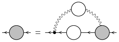
Figure 1: The exact Schwinger-Dyson equation for the quark propagator.

Setting $J^{a\mu}=\zeta=\overline{\zeta}=0$ after differentiating by $\zeta(y)$, we have the exact formula for the SD equation, which is shown in Fig.1. When we solve the exact equation for the quark propagator, we have to know the exact functional forms of the gluon propagator and the quark-gluon vertex function. In practical sense we need some approximation.

The ladder (or rainbow) approximation is to replace the quark-gluon vertex function and the gluon propagator with the tree vertex and the free propagator, respectively. The coupling is fixed constant. However, the approximated equation does not reproduce the property required by QCD. We regard the equation for QED rather than QCD.

In order to make the equation describe QCD theory, we incorporate the property of the asymptotic freedom into it by replacing the fixed coupling with the running coupling. The running coupling is given by the one-loop renormalization group equation usually. The renormalization point of the running coupling is essentially the gluon momentum squared, but as we will explain later several possibilities are allowed. The resultant approximations are called improved ladder (or rainbow) approximations.

Then, the Schwinger-Dyson equation in the improved ladder approximation is

$$iS_{F}^{-1}(p)=p\kern-6.0pt\mbox{\it/}-\int\!\!\frac{d^{4}k}{(2\pi)^{4}i}\>\frac{C_{2}g^{2}(p,k)}{-l^{2}}\left(g_{\mu\nu}-\eta(-l^{2})\frac{l_{\mu}l_{\nu}}{l^{2}}\right)\gamma^{\mu}iS_{F}(k)\gamma^{\nu}~{},$$ (2.2)

where $l_{\mu}=(p-k)_{\mu}$, $C_{2}=(N_{c}^{2}-1)/(2N_{c})$ is the second Casimir invariant, and $\eta(-l^{2})$ is the gauge fixing function.[18] For later convenience we have made the gauge parameter a function of $-l^{2}$, because it is possible to introduce a nonlocal gauge fixing function in gauge theories.

In general the quark propagator is expanded by two scalar functions

$$iS_{F}^{-1}(p)=A(-p^{2})p\kern-6.0pt\mbox{\it/}-B(-p^{2})~{}.$$ (2.3)

Substituting the eq.(2.3) into the Schwinger-Dyson equation (2.2), we have

$$(A(-p^{2})-1)p^{2} = \int\!\!\frac{d^{4}k}{(2\pi)^{4}i}\frac{C_{2}g^{2}(p,k)}{-l^{2}}\>\Bigg{[}\left(2+\eta(-l^{2})\right)p\cdot k$$

$$+2\eta(-l^{2})\frac{p^{2}k^{2}-(p\cdot k)^{2}}{-l^{2}}\Bigg{]}\frac{A(-k^{2})}{B(-k^{2})^{2}-A(-k^{2})^{2}k^{2}}~{},$$

$$B(-p^{2}) = \int\!\!\frac{d^{4}k}{(2\pi)^{4}i}\frac{(4-\eta(-l^{2}))C_{2}g^{2}(p,k)}{-l^{2}}$$ (2.4)

$$\times\frac{B(-k^{2})}{B(-k^{2})^{2}-A(-k^{2})^{2}k^{2}}~{}.$$

There are many possibilities for the argument of the running coupling constant $g^{2}(p,k)$. It is plausible to chose the argument such that the mass function

$$\Sigma(x)\equiv B(x)/A(x)~{},$$

be consistent with the result by the operator product expansion (OPE) at the high energy[3]

$$\Sigma(x)\sim\frac{g^{2}(x)}{x}\left(\ln\frac{x}{\mu^{2}}\right)^{1+\gamma_{{}_{\Sigma}}}\qquad\mbox{ for }~{}~{}x\sim\infty~{},$$ (2.5)

where

$$1+\gamma_{{}_{\Sigma}}=\frac{9C_{2}}{11N_{c}-2N_{f}}=\frac{4}{9}~{}.$$

When we discuss the dynamical symmetry breaking, the Lagrangian do never possess bare mass term. Starting from the chiral limit, however, non-perturbative approximation may violate chiral symmetry non-trivially. The existence of the bare mass $m_{0}$ modifies the high energy behavior of the system, especially $\Sigma(x)$ as $\sim m_{0}$ up to log corrections. So, in order to forbid bare mass to appear we require that the high energy behavior of the mass function be exactly the same as that in the case of vanishing bare mass.

Typical choices of the running coupling are

$$g^{2}(p,k)=\left\{\begin{array}[]{lc}g^{2}(\max(-p^{2},-k^{2}))&(\mbox{I})\\ g^{2}(-p^{2}-k^{2})&(\mbox{II})\\ g^{2}(-(p-k)^{2})&(\mbox{III})\end{array}\right.~{},$$ (2.6)

and all choices (I,II and III) reproduce the OPE result. The type (I) is first used by Higashijima and Miransky[4, 5]. In types (I) and (II) one can trivially carry out the angle integration of the Schwinger-Dyson equation (2.4) and reduce the equation to a simple one-dimensional integral equation. Moreover the quark propagator receives no wave function renormalization, $A(-p^{2})=1$, in the Landau gauge $\eta(-l^{2})=1$.[6] Thus performing the Wick rotation, we have

$$\Sigma(x)=\int_{0}^{\infty}\!\!ydy\>\frac{\lambda(x,y)}{\max(x,y)}\>\frac{\Sigma(y)}{y+\Sigma(y)^{2}}~{},$$ (2.7)

where

$$\lambda(x,y)=\frac{3C_{2}}{16\pi^{2}}\times\left\{\begin{array}[]{ll}g^{2}(\max(x,y))&\quad\mbox{for type (I)}\\ g^{2}(x+y)&\quad\mbox{for type (II)}\end{array}\right.$$ (2.8)

Especially in type (I) the Schwinger-Dyson equation (2.7) becomes a differential equation

$$\Bigg{[}\frac{\Sigma^{\prime}(x)}{(\lambda(x)/x)^{\prime}}\Bigg{]}^{\prime}=\frac{x\Sigma(x)}{x+\Sigma(x)^{2}}~{},$$ (2.9)

with appropriate boundary conditions.[4, 5, 6]

Next, we consider the type (III) which is the most natural since the chiral Ward-Takahashi identities hold in this case as explained later. We can always keep $A(-p^{2})=1$ using the freedom of the gauge function $\eta(-l^{2})$ in the type (III).[7] Let us explain this reason. From eq.(2.4)

$$(A-1)p^{2} = \int\!\!\frac{d^{4}k}{(2\pi)^{4}i}\>\frac{C_{2}g^{2}}{-l^{2}}$$

$$\Bigg{[}(2+\eta)p\cdot k+2\eta\frac{p^{2}k^{2}-(p\cdot k)^{2}}{-l^{2}}\Bigg{]}\>\frac{A}{B^{2}-A^{2}k^{2}}~{},$$

performing the Wick rotation and defining $x=-p^{2}$, $y=-k^{2}$, $z=-l^{2}=x+y-2\cos\theta\sqrt{xy}$, and $p\cdot k=-\cos\theta\sqrt{xy}$,

$$(A-1)p^{2} = -\frac{C_{2}}{12\pi^{3}}\int_{0}^{\infty}\!\!ydy\int_{0}^{\pi}\!\!d\theta\frac{\sin^{4}\theta}{z^{2}}\bigg{[}z\varphi^{\prime}(z)-2g^{2}(z)(\eta(z)-1)\bigg{]}\frac{A}{B^{2}-A^{2}k^{2}}~{},$$

where $\varphi(z)=g^{2}(z)(2+\eta(z))$ and the prime denotes differentiation. Therefore we can keep $A(x)\equiv 1$ as far as the gauge function $\eta(x)$ satisfies the differential equation

$$x\varphi^{\prime}(x)-2g^{2}(x)(\eta(x)-1)=0~{}.$$ (2.10)

Assuming that $g^{2}(x)$ is differentiable and finite, the differential equation (2.10) at $x=0$ gives the initial condition for itself:

$$0=0\times\varphi^{\prime}(0)-2g^{2}(0)(\eta(0)-1)~{},$$

thus

$$\eta(0)=1~{}.$$ (2.11)

The differential equation (2.10) means that the gauge function $\eta(x)$ can be determined without knowing the mass function $\Sigma(x)$.

Now, $B(x)$ becomes the mass function $\Sigma(x)$ itself, and from eq.(2.4) it is calculated by

$$\Sigma(x)=\int_{0}^{\infty}\!\!ydy\>K_{\Sigma}(x,y)\>\frac{\Sigma(y)}{y+\Sigma(y)^{2}}~{},$$ (2.12)

with

$$K_{\Sigma}(x,y)=\int_{0}^{\pi}\!\!d\theta\sin^{2}\theta\>\frac{C_{2}g^{2}(z)(4-\eta(z))}{8\pi^{3}z}~{}.$$ (2.13)

2.2 Vacuum Expectation Value of $\>\overline{q}q$

The vacuum expectation value (VEV) of the quark bilinear $\overline{q}q$ ($q=u,d$) is the simplest order parameter of the chiral symmetry;

$$\bigg{[}iQ_{5}^{a},\overline{\psi}i\gamma_{5}\frac{\tau^{b}}{2}\psi\bigg{]}=\delta^{ab}\frac{1}{2}\overline{\psi}\psi~{},$$ (2.14)

where $Q_{5}^{a}$ is the generator of the chiral rotation, $\tau^{b}$ is the Pauli matrix and $\psi=(u,d)^{T}$. Since $\overline{q}_{{}_{L}}q_{{}_{R}}$ transforms like $(2^{*},2)$ under $SU(2)_{L}\times SU(2)_{R}$, the VEV $\langle 0|\overline{q}q|0\rangle$ vanishes if the system is chiral invariant in the representation level. The symmetry in the representation level means the invariance which the vacuum has. When the system develops the non-vanishing VEV $\langle 0|\overline{\psi}\psi|0\rangle\neq 0$, the symmetry generated by the charge $Q_{5}^{a}$ breaks; $Q_{5}^{a}|0\rangle\neq 0$. $\langle 0|\overline{q}q|0\rangle\neq 0$ implies that the $\overline{q}q$ pair condensates in the vacuum. The symmetry of the vacuum under $SU(2)_{V}$ means that the VEVs of $\overline{u}u$ and $\overline{d}d$ are identical

$$\langle 0|\overline{u}u|0\rangle=\langle 0|\overline{d}d|0\rangle~{}.$$ (2.15)

Even when the system possesses the chiral symmetry in the Lagrangian level, there is no reason why the system keeps the symmetry in the representation level. Actually the chiral symmetry breaks spontaneously in QCD.[9, 10]

The VEV is calculated from the quark propagator

$$\langle 0|\overline{q}q|0\rangle_{\Lambda} = -N_{c}{\rm tr}S_{F}(x=0)$$ (2.16)

$$= -\frac{N_{c}}{4\pi^{2}}\int_{0}^{\Lambda^{2}}\!\!xdx\frac{\Sigma(x)}{x+\Sigma(x)^{2}}~{},$$

where $\Lambda$ is the Euclidean momentum cutoff. The VEV has ultra-violet divergence, and depends on the cutoff $\Lambda$. Instead, the renormalized VEV depends on the renormalization point $\mu^{2}$. Using the high energy behavior of the mass function (2.5), we identify the renormalized VEV $\langle 0|\overline{q}q|0\rangle_{\mu}$ by

$$\langle 0|\overline{q}q|0\rangle_{\mu}=\langle 0|\overline{q}q|0\rangle_{\Lambda}\>\left(\frac{g^{2}(\Lambda^{2})}{g^{2}(\mu^{2})}\right)^{1+\gamma_{\Sigma}}~{}.$$ (2.17)

We note that the quantity $\langle 0|\overline{q}q|0\rangle_{\Lambda}(g^{2}(\Lambda^{2}))^{1+\gamma_{\Sigma}}$ is independent of the cutoff $\Lambda$ for sufficiently large $\Lambda$.

The vacuum expectation value of the quark bilinear is certainly the simplest order parameter of the chiral symmetry, but needs renormalization of the ultraviolet divergence. The VEV is a notion which depends on a renormalization point. The most suitable order parameter of the chiral symmetry is, so-called, $L_{10}$ introduced by Gasser-Leutwyler[13]. If $L_{10}$ develops a non-zero value, the chiral symmetry breaks. This is a coefficient of the effective Lagrangian and suffers no ultraviolet divergence. Thus, the low-energy parameter $L_{10}$ does not depend on any renormalization point, and is well-defined. This low-energy parameter is evaluated in the improved ladder exact approximation in Ref. [14].

Using the current algebra technique, the VEV is expressed by the observable of the pion mass $m_{\pi}$, the pion decay constant $f_{\pi}$ and the current quark mass $\widehat{m}(\mu)\equiv(m_{u}(\mu)+m_{d}(\mu))/2$[11] in the lowest order perturbation of the quark masses

$$f_{\pi}^{2}m_{\pi}^{2}=-2\widehat{m}(\mu)\langle 0|\overline{q}q|0\rangle_{\mu}~{},$$ (2.18)

where the VEV is defined in the chiral limit. With the measured value of $m_{\pi}$ and $f_{\pi}$, and with the value $\widehat{m}(\mbox{1 GeV})=7\pm 2\mbox{ MeV}$ from the QCD sum rules for the axial divergence, we have an “experimental” value[12]

$$\langle 0|\overline{q}q|0\rangle_{{}_{\rm 1GeV}}=-(225\pm 25\mbox{ MeV})^{3}~{}.$$ (2.19)

The result in the improved ladder approximation is in good agreement with this result (2.19).

Before closing this subsection, we comment on another order parameter. One of the chiral coefficients, $L_{10}$, of so-called the S parameter is the finite order parameter, contrary to the VEV $\langle 0|\overline{q}q|0\rangle$: This is ultraviolet finite[13, 15, 16] and renormalization group invariant. We can measure the chiral symmetry or asymmetry without any ambiguity using this order parameter. However, the calculation of it in the improved ladder approximation is rather tedious as we will show later.

2.3 Chiral Ward-Takahashi Identities

We are considering the QCD with two massless quarks $u$ and $d$. Massless means vanishing bare (or current) mass here. This system possesses the $SU(2)_{L}\times SU(2)_{R}$ chiral symmetry. There are two Noether currents (vector and axial-vector) of this system

$$\partial_{\mu}J_{5}^{a\mu}=\partial_{\mu}J^{a\mu}=0~{},$$ (2.20)

where

$$J_{5}^{a\mu}=\overline{\psi}\gamma^{\mu}\gamma_{5}\frac{\tau^{a}}{2}\psi~{},\qquad J^{a\mu}=\overline{\psi}\gamma^{\mu}\frac{\tau^{a}}{2}\psi~{}.$$ (2.21)

By virtue of the current conservations, the chiral Ward-Takahashi (WT) identities hold formally. Of course one can check these WT identities hold in perturbation expansion. How is it in the case of the improved ladder approximation? The axial WT identity was first studied by Maskawa and Nakajima[18] in the ladder approximation with fixed coupling. The more detailed and complete analyses were made by Kugo and Mitchard[7, 8]. The improved ladder approximations in the type (I) and (II) ( see eq.(2.6)) slightly violate the identities, although the pion remains massless. This is because the axial Ward-Takahashi identity become hold in the soft pion limit $q_{\mu}\rightarrow 0$ with any type of the coupling choice (2.6)). We review the analyses in Refs. [7, 8].

The axial and vector Ward-Takahashi identities are

$$q^{\mu}\Gamma_{5\mu}^{a}(p;q) = \frac{\tau^{a}}{2}\left[iS_{F}^{-1}(p_{+})\gamma_{5}+\gamma_{5}iS_{F}^{-1}(p_{-})\right]~{},$$

$$q^{\mu}\Gamma_{\mu}^{a}(p;q) = \frac{\tau^{a}}{2}\left[iS_{F}^{-1}(p_{+})-iS_{F}^{-1}(p_{-})\right]~{},$$ (2.22)

where $p_{\pm}=p\pm q/2$. The basic ingredients in the chiral Ward-Takahashi identities are the quark propagator $S_{F}(p)$ and the three-point vertex functions of the vector and the axial currents, $\Gamma_{5\mu}^{a}(p;q)$ and $\Gamma_{\mu}^{a}(p;q)$ respectively. We studied about the quark propagators in the improved ladder approximation, but we do not about the three-point functions here. We only quote the inhomogeneous BS equations of them in the improved ladder approximation and postpone the derivation and discussions.

The Schwinger-Dyson equation reads

$$M(p)=\int\!\!\frac{d^{4}k}{(2\pi)^{4}i}K(p,k)iS_{F}(k)~{},$$ (2.23)

with

$$M(p)\equiv p\kern-6.0pt\mbox{\it/}-iS_{F}^{-1}(p)~{},$$ (2.24)

and $K$ is the BS kernel

$$K(p,k) = C_{2}g^{2}(p,k)D_{\mu\nu}(p-k)~{}\gamma^{\mu}\otimes\gamma^{\nu}{}~{},$$

$$D_{\mu\nu}(l) = \frac{1}{-l^{2}}\left(g_{\mu\nu}-\eta(-l^{2})\frac{l_{\mu}l_{\nu}}{l^{2}}\right)~{}.$$ (2.25)

We have used the tensor product notation:

$$(A\otimes B)\chi\equiv A\chi B~{}.$$ (2.26)

If the wave function renormalization factor is unity, $A(-p^{2})=1$, we have $M(p)=\Sigma(-p^{2})$. But we discuss the generic case $A(-p^{2})\neq 1$.

The inhomogeneous BS equation for the axial-vector vertex function $\Gamma_{5\mu}^{a}(p;q)$ in the improved ladder approximation is

$$\Gamma_{5\mu}^{a}(p;q)=\gamma_{\mu}\gamma_{5}\frac{\tau^{a}}{2}-\int\!\!\frac{d^{4}k}{(2\pi)^{4}i}K(p,k)\left(S_{F}(p_{+})\otimes S_{F}(p_{-})\right)\Gamma_{5\mu}^{a}(k;q)~{},$$ (2.27)

and the similar inhomogeneous BS equation for the vector vertex function $\Gamma_{\mu}^{a}(p;q)$ is hold. The vertex functions are defined by

$$\int\!\!dz~{}e^{iqz}~{}\langle 0|T\psi(x)\overline{\psi}(y)J_{5\mu}^{a}(z)|0\rangle=$$ (2.28)

$$e^{iq\frac{x+y}{2}}\int\!\!\frac{d^{4}p}{(2\pi)^{4}i}~{}e^{-ip(x-y)}~{}S_{F}(p_{+})\;\Gamma_{5\mu}^{a}(p;q)\;S_{F}(p_{-})~{},$$

and similarly for $\Gamma_{\mu}^{a}(p;q)$.

First we consider the axial WT identity. The formal solution of the inhomogeneous BS equation for the axial vertex function (2.27) is

$$\Gamma_{5\mu}^{a}(p;q)=\frac{1}{1-L}\gamma_{\mu}\gamma_{5}\frac{\tau^{a}}{2}~{},$$ (2.29)

where

$$L(p,k;q)=K(p,k)\;S_{F}(p_{+})\otimes S_{F}(p_{-})~{},$$ (2.30)

and we have used the “inner product” rule:

$$L\chi(p;q)\equiv\int\!\!\frac{d^{4}k}{(2\pi)^{4}i}~{}L(p,k;q)~{}\chi(k;q)~{}.$$ (2.31)

Multiplying the eq.(2.29) by $q^{\mu}$, we have

$$0=\frac{1}{1-L}q\kern-5.8pt\mbox{\it/}\gamma_{5}\frac{\tau^{a}}{2}-q^{\mu}\Gamma_{5\mu}^{a}(p;q)~{}.$$ (2.32)

Using the axial WT identity (2.22) and the following trivial identities

$$q\kern-5.8pt\mbox{\it/}\gamma_{5}\equiv iS_{F}^{-1}(p_{+})\gamma_{5}+\gamma_{5}iS_{F}^{-1}(p_{-})+M(p_{+})\gamma_{5}+\gamma_{5}M(p_{-})~{},$$

$$\frac{1}{1-L}-1\equiv\frac{1}{1-L}L~{},$$

we find

$$0=L\left(iS_{F}^{-1}(p_{+})\gamma_{5}+\gamma_{5}iS_{F}^{-1}(p_{-})\right)+\left(M(p_{+})\gamma_{5}+\gamma_{5}M(p_{+})\right)~{},$$ (2.33)

where we remove the overall factor

$$\left(\frac{\tau^{a}}{2}\right)\frac{1}{1-L}~{}.$$

The first term of eq. (2.33) is rewritten as the following:

$$L\left(iS_{F}^{-1}(p_{+})\gamma_{5}\right) = K\left(S_{F}(p_{+})\>iS_{F}^{-1}(p_{+})\gamma_{5}\>S_{F}(p_{-})\right)$$

$$= K\left(i\gamma_{5}S_{F}(p_{-})\right)$$

$$= -\gamma_{5}\left(KiS_{F}(p_{-})\right)~{},$$

and similarly

$$L\left(\gamma_{5}iS_{F}^{-1}(p_{-})\right)=-\left(KiS_{F}(p_{+})\right)\gamma_{5}~{}.$$

So, we can rewrite eq. (2.33) into

$$0=\left[\>M(p_{+})-KiS_{F}(p_{+})\>\right]\gamma_{5}+\gamma_{5}\left[\>M(p_{-})-KiS_{F}(p_{-})\>\right]~{}.$$ (2.34)

By tracing the same derivation for the axial vertex case, we obtain the similar identity like eq.(2.34) in the vector vertex case:

$$0=\left[\>M(p_{+})-KiS_{F}(p_{+})\>\right]-\left[\>M(p_{-})-KiS_{F}(p_{-})\>\right]~{}.$$ (2.35)

We can easily find that the only consistent manner is to require

$$M(p_{\mp}) = KiS_{F}(p_{\mp})$$ (2.36)

$$\equiv \int\!\!\frac{d^{4}k}{(2\pi)^{4}i}~{}K(p,k)~{}iS_{F}(k_{\mp})~{},$$

of the quark propagator. This equality reminds us with the Schwinger-Dyson equation (2.23), but there is a slight difference in the momentum flow. When we shift the momenta $p\rightarrow p\pm q/2$ and $k\rightarrow k\pm q/2$, the eq.(2.36) becomes

$$M(p)=\int\!\!\frac{d^{4}k}{(2\pi)^{4}i}~{}C_{2}g^{2}(p_{\pm},k_{\pm})D_{\mu\nu}(p-k)\gamma^{\mu}iS_{F}(k)\gamma^{\nu}~{},$$ (2.37)

where we consider only the case when the $k$-integration converges. Take the difference between this equation and the Schwinger-Dyson equation itself, we finally obtain

$$0=\int\!\!\frac{d^{4}k}{(2\pi)^{4}i}~{}C_{2}\bigg{(}~{}g^{2}(p_{\pm},k_{\pm})-g^{2}(p,k)~{}\bigg{)}D_{\mu\nu}(p-k)\gamma^{\mu}iS_{F}(k)\gamma^{\nu}~{}.$$ (2.38)

Thus, in order for the improved ladder approximation to be consistent with the chiral WT identities, we have to chose the argument of the running coupling such that

$$g^{2}(p_{\pm},k_{\pm})=g^{2}(p,k)~{},$$ (2.39)

holds. The type (III) is the only choice among the three candidates (2.6). The improved ladder approximation with the type (III) coupling choice is called the consistent ladder approximation. We should notice that any choices (2.6) satisfy (2.39) in the soft moemntum limit $q_{\mu}\rightarrow 0$.

Here we comment on the validity of momentum shift of the integration variable $k_{\mu}$ in eq. (2.36). When we solve the Schwinger-Dyson equation we perform the Wick rotation and use the momentum cutoff regularization usually. The obtained functions $A(-p^{2})$ and $B(-p^{2})$ which satisfy the SD equation identically make the integration in the eq. (2.37) convergent enough. As for the high energy momentum of the $k_{\mu}$, we are allowed to ignore the momentum $q_{\mu}$ in the integrand of eq. (2.36). Even in the fixed coupling case the momentum integration of the Schwinger-Dyson equation is convergent one, because we calculate the function $A$ and $B$ by the following way. The fixed coupling is regarded as the function in the cutoff. We tune the coupling to the critical value as the cutoff goes to infinity so as for the function $A(-p^{2})$ and $B(-p^{2})$ become finite. Thus, the high energy behavior of the integrand in the RHS of the eq.(2.36) or eq.(2.37) is

$$\sim C_{2}g^{2}(p,k)D_{\mu\nu}(p-k)\gamma^{\mu}iS_{F}(k)\gamma^{\nu}\qquad\mbox{ as }-\!k^{2}\longrightarrow\infty~{}.$$ (2.40)

This behavior is identically the same as that for the Schwinger-Dyson equation itself which has convergent integral by construction. We conclude that the violation of the chiral WT identities due to the momentum shift vanishes.

2.4 Pagels-Stokar Formula

Within the knowledge of the mass function $\Sigma(x)$, we can estimate the pion decay constant $f_{\pi}$ using the Pagels-Stokar formula[17]

$$f_{\pi}^{2}=\frac{N_{c}}{4\pi^{2}}\int_{0}^{\infty}\!\!xdx\>\frac{\Sigma(x)(\Sigma(x)-\frac{x}{2}\Sigma^{\prime}(x))}{(x+\Sigma(x)^{2})^{2}}{}~{}.$$ (2.41)

If one use $f_{\pi}$ as an input parameter of the mass dimension, the output is $\Lambda_{\rm QCD}$.

Following Pagels and Stokar, we derive the formula. The pion decay constant $f_{\pi}$ is defined by

$$\Big{\langle}0\Big{|}\overline{\psi}\gamma_{\mu}\gamma_{5}\frac{\tau^{a}}{2}\psi(0)\Big{|}\pi^{b}(q)\Big{\rangle}=\delta^{ab}iq_{\mu}\>f_{\pi}~{}.$$ (2.42)

Using the definition of the pion BS amplitude (2.49) we rewrite into

$$f_{\pi}\>q_{\mu}=-\frac{N_{c}}{2}\int\!\!\frac{d^{4}p}{(2\pi)^{4}i}~{}{\rm tr}\left[\gamma_{\mu}\gamma_{5}\chi(p;q)\right]~{}.$$ (2.43)

The factor $1/2$ comes from ${\rm tr}[(\tau^{a}/2)(\tau^{b}/2)]=\delta^{ab}/2$. In order to calculate $f_{\pi}$ we need the BS amplitude only in the order $O(q_{\mu})$ since $q^{2}=0$. In the soft momentum limit, the BS amplitude is indeed expressed in terms of the mass function by virtue of the axial Ward-Takahashi identity.

In any choices of the running coupling (2.6) the axial Ward-Takahashi identity is satisfied

$$q^{\mu}\Gamma_{5\mu}^{a}(p;q)=iS_{F}^{-1}(p+{\scriptstyle\frac{1}{2}}q)\gamma_{5}\frac{\tau^{a}}{2}+\frac{\tau^{a}}{2}\gamma_{5}iS_{F}^{-1}(p-{\scriptstyle\frac{1}{2}}q)~{},$$ (2.44)

where $\Gamma_{5\mu}^{a}(p;q)$ is the axial vertex function defined by eq.(2.28). Substituting the quark propagator in the improved ladder approximation $iS_{F}^{-1}(p)=p\kern-6.0pt\mbox{\it/}-\Sigma(-p^{2})$ into the axial WT identity (2.44), we obtain, in the soft momentum limit $q_{\mu}\rightarrow 0$,

$$\lim_{q_{\mu}\rightarrow 0}q^{\mu}\Gamma_{5\mu}^{a}(p;q)=-\tau^{a}\gamma_{5}\Sigma(-p^{2})~{}.$$ (2.45)

The eq.(2.45) shows that the soft pion contribution to the axial vertex function is completely determined by the mass function. Namely, the axial WT identity fixes the contribution of the soft pion to the axial vertex function.

In general the axial vertex function is decomposed into two parts; the singular part due to the massless pion pole and the regular part

$$\Gamma_{5\mu}^{a}(p;q)\sim-\left(\frac{\tau^{a}}{2}\right)\widehat{\chi}(p;q)\>\frac{f_{\pi}q_{\mu}}{q^{2}}+\mbox{ regular at $q^{2}\rightarrow 0$}~{},$$ (2.46)

where $\widehat{\chi}(p;q)$ is the amputated BS amplitude. From eqs.(2.45) and (2.46) we have

$$\widehat{\chi}(p;q\rightarrow 0)=-\gamma_{5}\frac{2\Sigma(-p^{2})}{f_{\pi}}{}~{}.$$ (2.47)

Pagels and Stokar made a glorious approximation that the amputated BS amplitude up to the order $O(q_{\mu})$ be given by eq. (2.47). Thus, we find

$$\chi(p;q) = S_{F}(p+{\scriptstyle\frac{1}{2}}q)\widehat{\chi}(p;q)S_{F}(p-{\scriptstyle\frac{1}{2}}q)$$ (2.48)

$$\cong S_{F}(p+{\scriptstyle\frac{1}{2}}q)\left(-\gamma_{5}\frac{2\Sigma(-p^{2})}{f_{\pi}}\right)S_{F}(p-{\scriptstyle\frac{1}{2}}q)~{}.$$

Substituting the BS amplitude (2.48) into the definition of $f_{\pi}$ (2.43), we obtain the desired formula (2.41).

2.5 Bethe-Salpeter Equation for the Pion

In this section we study the Bethe-Salpeter equation for the pion with improved ladder approximation. In order to evaluate the pion decay constant $f_{\pi}$, the BS amplitude of the pion is calculated. This calculation has been done by two groups[6, 19] first. The pion appears as the massless particle in the Bethe-Salpeter equation. The more detailed analyses were made in Refs. [8, 20] followingly. The improved ladder approximation which is consistent with the chiral Ward-Takahashi identities is found in Refs.[7, 8].

The Nambu-Goldstone’s theorem[9, 21] guarantees that the pion appears as an massless particle, where the system possesses the chiral symmetry. However the above studies tell us that massless-ness of the pion is guaranteed by what one use the same BS kernel in the SD and BS equations simultaneously. To use the same BS kernel is, of course, leads to the WT identity of the chiral symmetry in the soft momentum limit $q_{\mu}\rightarrow 0$ on account of (2.39). This point is discussed in subsection 2.3. If the pion could not appear as a massless particle, the BS equation would have no solution at zero momentum-squared $q^{2}=0$. In what follows we show the equation indeed has the solution at $q^{2}=0$.

The BS amplitude $\chi$ and the truncated BS amplitude $\widehat{\chi}$ for the pion are defined by

$$\Big{\langle}0\Big{|}T\psi_{i}(\frac{-r}{2})\overline{\psi}^{j}(\frac{r}{2})\Big{|}\pi^{a}(q)\Big{\rangle} = {\cal N}\delta_{i}^{j}\frac{\tau^{a}}{2}~{}\int\!\!\frac{d^{4}p}{(2\pi)^{4}i}~{}e^{-ipr}~{}\chi(p;q)~{},$$

$$\widehat{\chi}(p;q) = S_{F}^{-1}(p_{+})~{}\chi(p;q)~{}S_{F}^{-1}(p_{-})~{},$$ (2.49)

where $p_{\pm}=p\pm q/2$, $i,j$ are color indices and ${\cal N}$ is a constant introduced for later convenience. When we put ${\cal N}=1$, these equations give the usual definitions for the BS amplitude and its truncated one. The Kronecker delta $\delta_{i}^{j}$ reflects the fact that mesons are color singlet. Taking into account of the spinor structure and the quantum numbers $J^{PC}=0^{-+}$, the (truncated) BS amplitude is expanded by four invariant amplitudes, i.e., $S,P,\cdots,\widehat{Q},\widehat{R}$, as

$$\chi(p;q)\gamma_{5} = S(p;q)+(p\cdot q)p\kern-6.0pt\mbox{\it/}P(p;q)+q\kern-5.8pt\mbox{\it/}Q(p;q)+{\scriptstyle\frac{1}{2}}[p\kern-6.0pt\mbox{\it/},q\kern-5.8pt\mbox{\it/}]R(p;q)~{},$$

$$\widehat{\chi}(p;q)\gamma_{5} = \widehat{S}(p;q)+(p\cdot q)p\kern-6.0pt\mbox{\it/}\widehat{P}(p;q)+q\kern-5.8pt\mbox{\it/}\widehat{Q}(p;q)+{\scriptstyle\frac{1}{2}}[p\kern-6.0pt\mbox{\it/},q\kern-5.8pt\mbox{\it/}]\widehat{R}(p;q)~{}.$$ (2.50)

Using the charge conjugation, it is easy to see that the every invariant amplitude $X=S$, $P$, $\cdots$, $\widehat{Q}$, $\widehat{R}$ is an even function in $(p\!\cdot\!q)$.

Our aim is to calculate the pion decay constant $f_{\pi}$ from the BS amplitude. The definition of $f_{\pi}$ is

$$f_{\pi}~{}iq_{\mu}\delta^{ab} \equiv \langle 0|\overline{\psi}\gamma_{\mu}\gamma_{5}\frac{\tau^{a}}{2}\psi(0)|\pi^{b}(q)\rangle$$ (2.51)

$$= -\>{\cal N}\frac{\delta^{ab}}{2}N_{c}\int\!\!\frac{d^{4}p}{(2\pi)^{4}i}~{}{\rm tr}\left[\gamma_{\mu}\gamma_{5}\chi(p;q)\right]~{}.$$

The second equality in eq.(2.51) is obtained by taking the trace on the definition (2.49) of $\chi$ with $\gamma_{\mu}\gamma_{5}\tau^{b}/2$ multiplied. It is easy to see from eq.(2.51) that we are enough to calculate the BS amplitude up to $O(q_{\mu})$ for the purpose of calculating the decay constant $f_{\pi}$. So, we expand the BS amplitude in powers of $q_{\mu}$ and keep them up to $O(q_{\mu})$:

$$\chi(p;q)=\chi^{0}(p)+q^{\mu}\chi_{\mu}(p)+O(p\cdot q)^{2}~{},$$ (2.52)

with

$$\chi^{0}(p) = \gamma_{5}\;S(-p^{2})~{},$$

$$\chi_{\mu}(p) = p_{\mu}p\kern-6.0pt\mbox{\it/}\gamma_{5}\;P(-p^{2})+\gamma_{\mu}\gamma_{5}\;Q(-p^{2})+{\scriptstyle\frac{1}{2}}[p\kern-6.0pt\mbox{\it/},\gamma_{\mu}]\gamma_{5}\;R(-p^{2})~{},$$ (2.53)

and similarly for $\widehat{\chi}(p;q)$. The invariant amplitude $X=S$, $P$, $\cdots$, $\widehat{Q}$, $\widehat{R}$ is also expanded as

$$X(p;q)=X(-p^{2})+O(p\cdot q)^{2}~{}.$$ (2.54)

Next we show how the BS amplitude is calculated from the BS equation. The homogeneous Bethe-Salpeter equation for the pion reads

$$(T-K)\>\chi(p;q)=0~{},\qquad(q^{2}=0)~{},$$ (2.55)

where $K$ is the BS kernel defined previously by eq.(2.25) which represents one-gluon exchange and $T$ is the kinetic part defined by

$$T(p;q)=S_{F}^{-1}(p_{+})\otimes S_{F}^{-1}(p_{-})~{},$$ (2.56)

where $p_{\pm}=p\pm q/2$. We use the tensor product notation (2.26) and the inner product rule (2.31). We notice that the homogeneous equation (2.55) tell us nothing about the normalization of the BS amplitude itself, and we need the normalization condition.

We solve the BS equation (2.55) order by order in $q_{\mu}$. The BS equation (2.55) is expanded in powers of $q_{\mu}$, and the equality is hold at each order in $q_{\mu}$. Namely,

$$(T^{0}+q^{\mu}T_{\mu}-K)\>(\chi^{0}+q^{\mu}\chi_{\mu})=0+O(p\cdot q)^{2}~{}.$$

$$\Downarrow$$

$$O(1): (T^{0}-K)\>\chi^{0}=0~{},$$ (2.57)

$$O(q_{\mu}): (T^{0}-K)\>\chi_{\mu}=-T_{\mu}\chi^{0}~{}.$$ (2.58)

The kinetic part $T$ is expanded as

$$T(p;q)=T^{0}(p)+q^{\mu}T_{\mu}(p)+O(p\cdot q)^{2}~{},$$ (2.59)

with

$$T^{0}(p) \equiv T(p;q)\bigg{|}_{\displaystyle q_{{}_{\lambda}}=0}$$

$$= -(p\kern-6.0pt\mbox{\it/}-\Sigma(-p^{2}))\otimes(p\kern-6.0pt\mbox{\it/}-\Sigma(-p^{2}))~{},$$

$$T_{\mu}(p) \equiv \frac{\partial}{\partial q^{\mu}}T(p;q)\bigg{|}_{\displaystyle q_{{}_{\lambda}}=0}~{},$$ (2.60)

$$= (p\kern-6.0pt\mbox{\it/}-\Sigma(-p^{2}))\otimes({\scriptstyle\frac{1}{2}}\gamma_{\mu}+p_{\mu}\Sigma^{\prime}(-p^{2}))$$

$$-({\scriptstyle\frac{1}{2}}\gamma_{\mu}+p_{\mu}\Sigma^{\prime}(-p^{2}))\otimes(p\kern-6.0pt\mbox{\it/}-\Sigma(-p^{2}))~{},$$

where $\Sigma^{\prime}(x)=d\Sigma(x)/dx$.

First we solve the $O(1)$ BS equation (2.57). This equation means that the operator $T^{0}-K$ has zero eigenvalue on the subspace expanded by $S(-p^{2})$. We find the solution of this equation if we put $\widehat{S}(x)\propto\Sigma(x)$. We show this point. It is easy to see that after performing the Wick rotation we have

$$T^{0}\chi^{0} = -\gamma_{5}(x+\Sigma(x)^{2})\>S(x)~{},$$

$$K\chi^{0} = -\gamma_{5}\int_{0}^{\infty}\!\!ydy~{}K_{\Sigma}(x,y)S(y)~{},$$ (2.61)

where $x=-p^{2}$ and $K_{\Sigma}$ is defined by eq.(2.13). The relation between $\chi^{0}$ and $\widehat{\chi}^{0}$ gives (see also the appendix A)

$$-\widehat{S}(x)=(x+\Sigma(x)^{2})S(x)\qquad\longleftrightarrow\qquad S(x)=-\frac{\widehat{S}(x)}{x+\Sigma(x)^{2}}~{}.$$ (2.62)

Substituting eqs. (2.61) and (2.62) into the $O(1)$ BS equation (2.57), we obtain the linear equation in terms of $\widehat{S}$

$$\widehat{S}(x)=\int_{0}^{\infty}\!\!\!ydy~{}K_{\Sigma}(x,y)\frac{\widehat{S}(y)}{y+\Sigma(y)^{2}}~{}.$$ (2.63)

This equation reminds us with the Schwinger-Dyson equation (2.12). Clearly $\widehat{S}(x)\propto\Sigma(x)$ is a solution and in fact this is the unique solution from the consequence of the axial Ward-Takahashi identity in the soft momentum limit (2.45). To say more detail, the axial Ward-Takahashi identity (2.22) uniquely determine the solution as well as the normalization constant of the BS amplitude in the soft momentum limit $q_{\mu}\rightarrow 0$. We already derive the normalization constant in eq. (2.47). Taking into account the proportional constant ${\cal N}$ in eq.(2.47), when we put ${\cal N}=-2/f_{\pi}$ we have a important relation

$$\widehat{S}(x)=\Sigma(x)~{}.$$ (2.64)

Second we solve the $O(q_{\mu})$ BS equation (2.58). Once we obtain $\chi^{0}$, i.e., eq.(2.64), the $O(q_{\mu})$ BS equation is regarded as a inhomogeneous equation for $\chi_{\mu}$ with the inhomogeneous term $-T_{\mu}\chi^{0}$. The formal solution of eq. (2.58) is

$$\chi_{\mu}=\frac{-1}{T^{0}-K}\>T_{\mu}\chi^{0}~{}.$$ (2.65)

Let us define the formal solution (2.65) in the constructive way. It is convenient to rewrite the invariant amplitudes and the spinor base of eq.(2.50) in the compact forms:

$$\begin{array}[]{rcl}\chi^{i}&\equiv&(P,Q,R)~{},\\ \Gamma_{i\mu}&\equiv&(\;p_{\mu}p\kern-6.0pt\mbox{\it/}\gamma_{5}\;,~{}\gamma_{\mu}\gamma_{5}\;,~{}{\scriptstyle\frac{1}{2}}[p\kern-6.0pt\mbox{\it/},\gamma_{\mu}]\gamma_{5}\;)~{},\end{array}\qquad(i=1,2,3)$$ (2.66)

where we find

$$\chi_{\mu}(p)=\Gamma_{i\mu}(p)\chi^{i}(-p^{2})~{}.$$ (2.67)

We introduce the matrix representations for $T^{0}$, $T_{\mu}$ and $K$:

$$T^{0}_{ij}(x) \equiv \frac{1}{4}{\rm tr}\left[\>\overline{\Gamma}_{i}^{\mu}(p)T^{0}(p)\Gamma_{j\mu}(p)\>\right]~{},$$

$$\lambda_{i}(x) \equiv \frac{1}{4}{\rm tr}\left[\>\overline{\Gamma}_{i}^{\mu}(p)T_{\mu}(p)\gamma_{5}\>\right]~{},$$

$$K_{ij}(x,y) \equiv \frac{1}{8\pi^{3}}\int_{0}^{\pi}\!\!d\theta\sin^{2}\theta~{}\frac{1}{4}{\rm tr}\left[\>\overline{\Gamma}_{i}^{\mu}(p)K(p,k)\Gamma_{j\mu}(k)\>\right]~{}.$$ (2.68)

The quantity $\overline{\Gamma}$ is the Dirac conjugate of $\Gamma$ before performing the Wick rotation; i.e., in general

$$\overline{\chi}(p;q)\equiv\gamma^{0}\chi(p^{*};q)^{\dagger}\gamma^{0}\qquad\mbox{for}\quad{}^{\forall}\chi~{}.$$ (2.69)

The detailed expressions of $T^{0}_{ij}$, $\lambda_{i}$ and $K_{ij}$ are summarized in the appendix A. With the matrix representations eq.(2.68) the $O(q_{\mu})$ BS equation is rewritten into a component form. Multiplied by $(1/4){\rm tr}[\overline{\Gamma}_{i}^{\mu}\times~{}]$ from left, the $O(q_{\mu})$ BS equation (2.58) reads

$$\frac{1}{4}{\rm tr}\left[\>\overline{\Gamma}_{i}^{\mu}\;(T^{0}-K)\;\Gamma_{j\mu}\>\right]\>\chi^{j}=-\frac{1}{4}{\rm tr}\left[\>\overline{\Gamma}_{i}^{\mu}\;T_{\mu}\;\gamma_{5}\>\right]S$$

$$\Downarrow$$

$$T^{0}_{ij}(x)\;\chi^{j}(x)-\int_{0}^{\infty}\!\!ydy~{}K_{ij}(x,y)\;\chi^{j}(y)=\frac{\Sigma(x)}{x+\Sigma(x)^{2}}\;\lambda_{i}(x)~{}.$$ (2.70)

The notable property is that the matrices $T^{0}$, $K$ are self conjugate and real definite

$$\begin{array}[]{ccccc}T^{0}(x){}^{\dagger}&=&T^{0}(x){}^{T}&=&T^{0}(x)~{},\\ K(x,y)^{\dagger}&=&K(x,y)^{T}&=&K(y,x)~{}.\end{array}$$ (2.71)

This is the direct consequence of the charge conjugation properties of the base $\Gamma_{i\mu}(p)$. We see from the property (2.71) that we obtain the real definite BS amplitude $\chi^{i}(x)$. It is not difficult to solve this inhomogeneous linear equation numerically by iteration method.

Finally we make a comment on the inverse operator of $T^{0}-K$ (cf. eq.(2.65)) which we need for solving the BS equation (2.70). One might be afraid that the operator $T^{0}-K$ had a zero eigenvalue suggested by eq.(2.57), and its inverse did not exist. However, one can understand that it is not the case because of the following reason.

Let us define the four Hilbert spaces $\SS$, ${\cal P}$, ${\cal Q}$, ${\cal R}$ as

$$\begin{array}[]{ll}\SS=\{~{}\gamma_{5}\>S(x)~{}\}~{},&{\cal P}=\{~{}\Gamma_{1\mu}\>P(x)~{}\}~{},\\ {\cal Q}=\{~{}\Gamma_{2\mu}\>Q(x)~{}\}~{},&{\cal R}=\{~{}\Gamma_{3\mu}\>R(x)~{}\}~{},\end{array}$$ (2.72)

which are spanned by any functions $S(x)$, $P(x)$, $Q(x)$ and $R(x)$. Then

$$\begin{array}[]{llll}\chi^{0}\in\SS~{},&\chi_{1\mu}\in{\cal P}~{},&\chi_{2\mu}\in{\cal Q}~{},&\chi_{3\mu}\in{\cal R}~{},\\ \chi_{\mu}\in{\cal P}{\cal Q}{\cal R}~{},&\chi\in{\cal P}{\cal Q}{\cal R}\SS~{},&&\end{array}$$ (2.73)

where ${\cal P}{\cal Q}{\cal R}\equiv{\cal P}\oplus{\cal Q}\oplus{\cal R}$ and so on. The spaces $\SS$, ${\cal P}{\cal Q}$ and ${\cal R}$ are orthogonal with each other in a sense that

$$\begin{array}[]{cccc}{\rm tr}\left[\overline{\gamma}_{5}\Gamma_{i\mu}\right]=0&(i=1,2,3)&\longrightarrow&\SS\perp{\cal P}{\cal Q}~{},{\cal R}\\ {\rm tr}\left[\overline{\Gamma}_{3}^{\mu}\Gamma_{i\mu}\right]=0&(i=1,2)&\longrightarrow&{\cal R}\perp{\cal P}{\cal Q}~{}.\end{array}$$ (2.74)

It is not difficult to check (cf. matrix forms in appendix A) that these orthogonalities conclude that the multiplications of the subspaces $\SS$, ${\cal P}$, ${\cal Q}$, ${\cal R}$ by the operators $T^{0}$, $T_{\mu}$ generate transitions between those spaces as

$$\begin{array}[]{ll}T^{0}\hookrightarrow\SS~{},&T^{0}\hookrightarrow{\cal P}{\cal Q}{\cal R}~{},\\ T_{\mu}:\SS\rightarrow S\cup{\cal P}{\cal Q}{\cal R}~{},&T_{\mu}\hookrightarrow{\cal P}{\cal Q}{\cal R}~{},\end{array}$$ (2.75)

where $T\hookrightarrow X$ means $T:X\rightarrow X$. To say more concretely, for example, $T^{0}\chi^{0}$ is a element in the subspace $\SS$ and so on. Thus, ${\cal P}{\cal Q}{\cal R}$ is a subspace; i.e., it is closed under the multiplications by $T^{0}$ and $T_{\mu}$, and $\SS$ is a quotient space. We note that the multiplication of $\SS$ by $T_{\mu}$ generate inhomogeneous part in ${\cal P}{\cal Q}{\cal R}$. Similarly, it is easy to see (cf. the appendix A) that

$$\begin{array}[]{ccc}K\hookrightarrow\SS~{},&K\hookrightarrow{\cal P}{\cal Q}~{},&K\hookrightarrow{\cal R}~{}.\end{array}$$ (2.76)

$\SS$, ${\cal P}{\cal Q}$ and ${\cal R}$ are closed under the multiplication by $K$. Namely, ${\cal P}{\cal Q}{\cal R}$ is closed under the multiplications by $T^{0}$, $T_{\mu}$ and $K$, and especially $\SS$ is also closed by means of quotient space. Therefore we conclude the eq.(2.58) can be solved on the subspace ${\cal P}{\cal Q}{\cal R}$ and the zeros of the operator $T^{0}-K$ in $\SS$ does not bring about that in ${\cal P}{\cal Q}{\cal R}$.

3 The Low Energy Parameter $L_{10}$ in QCD and S Parameter

Strong interactions of the light degrees of freedom respect chiral symmetry. The symmetrical aspects of the strong interaction are expressed in terms of the chiral Lagrangian. There are ten low-energy parameters $L_{1}$, $\cdots$, $L_{10}$ which are introduced by Gasser-Leutwyler[13] besides the pion decay constant $f_{\pi}$. The S parameter in QCD is related to one of the low-energy parameters $L_{10}$ by the ratio $S=-16\pi L_{10}$. The S parameter is a finite order parameter of the chiral symmetry[16] while the vacuum expectation value of the quark bilinear suffers ultraviolet divergence and is to be regularized.

In this section we calculate the low-energy parameter $L_{10}$, or so-called S parameter $S$ in QCD, and the pion decay constant $f_{\pi}$, using the inhomogeneous BS equation in the improved ladder approximation. In order to hold the chiral symmetry, we keep the same approximation to the SD equation which determines the quark mass function. The obtained mass function is used in the inhomogeneous BS equation. The QCD S parameter $S$ and the pion decay constant $f_{\pi}$ are evaluated, in the chiral limit, from the current two-point function of ‘V-A’ type $\Pi_{VV}(q^{2})-\Pi_{AA}(q^{2})$ in the space-like region.

3.1 QCD S Parameter and Two-Point Function

In order to calculate the ‘V-A’ tow-point function $\Pi_{VV}(q^{2})-\Pi_{AA}(q^{2})$ we consider the vector and axial-vector currents $V^{a}_{\mu}(x)$ and $A^{a}_{\mu}(x)$ defined by

$$V^{a}_{\mu} = \overline{\psi}\frac{\tau^{a}}{2}\gamma_{\mu}\psi~{},$$

$$A^{a}_{\mu} = \overline{\psi}\frac{\tau^{a}}{2}\gamma_{\mu}\gamma_{5}\psi~{},$$ (3.1)

where $\psi=(u,d)^{T}$ and $\tau^{a}$ ($a\!=\!1,2,3$) is Pauli matrix. The two-point functions $\Pi_{JJ}$ of the current $J^{a}_{\mu}$ ($=V^{a}_{\mu},A^{a}_{\mu}$) is given by

$$\delta^{ab}\Pi_{JJ}(q^{2})=\epsilon^{\mu}\epsilon^{\nu}i\int d^{4}xe^{iqx}\langle 0|TJ^{a}_{\mu}(x)J^{b}_{\nu}(0)|0\rangle~{},$$ (3.2)

where $\epsilon^{\mu}$ is the polarization vector defined by $\epsilon\!\cdot\!q=0$, $\epsilon^{2}=-1$. The QCD S parameter $S$ and pion decay constant $f_{\pi}$ are calculated using the two-point function as

$$S = 4\pi\frac{d}{dq^{2}}\Big{[}\Pi_{VV}(q^{2})-\Pi_{AA}(q^{2})\Big{]}\bigg{|}_{q^{2}=0}~{},$$

$$f_{\pi}^{2} = \Pi_{VV}(0)-\Pi_{AA}(0)~{}.$$ (3.3)

First one of eq. (3.3) is the definition of the QCD S parameter, and second one is derived from the definition of $f_{\pi}$ using QCD sum rule. In what follows, the isospin indices $a,b,\cdots$ are suppressed for simplicity.

Let us derive the sum rules of the quantities $S$ and $f_{\pi}$. We expand the two-point Wightman function $W_{\mu\nu}(x)$ of the current $J_{\mu}$ by using the physical complete set $1=\sum_{n}|n\rangle\langle n|$, and we insert the identity $1=\int\!d^{4}q~{}\delta^{4}(q-q_{n})$ in the summand. Thus,

$$W_{\mu\nu}(x) \equiv \langle 0|J_{\mu}(x)J_{\nu}(0)|0\rangle$$ (3.4)

$$= \sum_{n}\langle 0|J_{\mu}(0)|n\rangle e^{-iq_{n}x}\langle n|J_{\nu}(0)|0\rangle$$

$$= \int d^{4}qe^{-iqx}\sum_{n}\delta^{4}(q-q_{n})\langle 0|J_{\mu}|n\rangle\langle n|J_{\nu}|0\rangle~{},$$

where $q_{n}^{\mu}$ is the momentum of the state $|n\rangle$ and we use the short hand notation $\langle 0|J_{\mu}(0)|n\rangle=\langle 0|J_{\mu}|n\rangle$. When we consider in the rest frame ($\vec{q}_{n}=0$) of the massive state $|n\rangle$, we find

$$\langle 0|J_{\mu}|n\rangle=0~{},$$ (3.5)

otherwise $\mu\!=\!0$ and $|n\rangle$ is scalar state, or $\mu\!\neq\!0$ and $|n\rangle$ is vector state. This follows from the fact that the quantity $\langle 0|J_{\mu}|n\rangle$ has to be a scalar. Here, scalar and vector are the notions of the three-dimensional continuous rotation in the rest frame of $|n\rangle$. The states which appears in the summand of eq. (3.4) survive if and only if those are spin-$0$ or spin-$1$ states. The Wightman function $W_{\mu\nu}(x)$ consists of spin-$0$ part $W_{\mu\nu}^{(0)}(x)$ and spin-$1$ part $W_{\mu\nu}^{(1)}(x)$ as

$$W_{\mu\nu}(x)=W_{\mu\nu}^{(0)}(x)+W_{\mu\nu}^{(1)}(x)~{}.$$ (3.6)

We define the Fourier transform of $W_{\mu\nu}(x)$ as

$$W_{\mu\nu}(q)=\int\!\frac{d^{4}x}{2\pi}~{}e^{iqx}~{}W_{\mu\nu}(x)~{},$$ (3.7)

and similarly for $W_{\mu\nu}^{(0)}(x)$ and $W_{\mu\nu}^{(1)}(x)$.

Massive spin-$0$ particles do not couple to conserved currents because $0$ = $q^{\mu}\langle 0|J_{\mu}|n\rangle$ = $q^{0}\langle 0|J_{0}|n\rangle$ in the rest frame. Massless spin-$0$ particles can couple to conserved currents, which defines the decay constant

$$\langle 0|J_{\mu}|n\rangle=iq_{\mu}\,f_{n}^{(0)}~{}.$$ (3.8)

We know only the pion as such particles, thus

$$\langle 0|A_{\mu}|\pi\rangle=iq_{\mu}\,f_{\pi}~{},$$ (3.9)

and $f_{n}^{(0)}=0$ for others. Then, the spin-$0$ part of the Wightman function $W^{(0)}(x)$ is given as

$$W_{\mu\nu}^{(0)}(q) = (2\pi)^{3}\sum_{n}\delta^{4}(q-q_{n})\langle 0|A_{\mu}(x)|n\rangle\langle n|A_{\nu}(0)|0\rangle$$ (3.10)

$$= (2\pi)^{3}\int\frac{d^{4}q^{\prime}}{(2\pi)^{3}}\theta(q^{\prime}{}^{0})\delta(q^{\prime}{}^{2})\delta^{4}(q-q^{\prime})\Big{(}-f_{\pi}^{2}q_{\mu}q_{\nu}\Big{)}$$

$$= -f_{\pi}^{2}~{}\theta(q^{0})\delta(q^{2})\;q_{\mu}q_{\nu}~{},$$

where $n$ runs over all spin 0 states.

The decay constants of massive spin-$1$ particles are defined by

$$\langle 0|J_{\mu}|n,\epsilon\rangle=\epsilon_{\mu}~{}f_{n}^{(1)}m_{n}~{},$$ (3.11)

where $m_{n}$ is the mass and $\epsilon^{\mu}$ is the polarization vector of the state $|n\rangle$ which satisfies $\epsilon\!\cdot\!q_{n}=0$ and $\epsilon^{2}\!=\!-1$. Of course, continuum states also have couplings $f_{n}^{(1)}$. Summing over the polarizations, we have

$$\sum_{\epsilon}\langle 0|J_{\mu}|n,\epsilon\rangle\langle n,\epsilon|J_{\nu}|0\rangle = \sum_{\epsilon}\epsilon_{\mu}\epsilon_{\nu}\Big{|}f_{n}^{(1)}m_{n}\Big{|}^{2}$$ (3.12)

$$= \left(-g_{\mu\nu}+\frac{q_{n\mu}q_{n\nu}}{q_{n}^{2}}\right)\Big{|}f_{n}^{(1)}m_{n}\Big{|}^{2}~{}.$$

Then, we obtain

$$W_{\mu\nu}^{(1)}(q) = (2\pi)^{3}\sum_{n}\delta^{4}(q-q_{n})\langle 0|J_{\mu}(x)|n,\epsilon\rangle\langle n,\epsilon|J_{\nu}(0)|0\rangle$$ (3.13)

$$= (2\pi)^{3}\sum_{n}\int\frac{d^{4}q_{n}}{(2\pi)^{3}}\theta(q_{n}^{0})\delta(q_{n}^{2}-m_{n}^{2})\times\delta^{4}(q-q_{n})\left(-g_{\mu\nu}+\frac{q_{\mu}q_{\nu}}{q^{2}}\right)\Big{|}f_{n}^{(1)}m_{n}\Big{|}^{2}~{}$$

$$= \sum_{n}\Big{|}f_{n}^{(1)}m_{n}\Big{|}^{2}\left(-g_{\mu\nu}+\frac{q_{\mu}q_{\nu}}{q^{2}}\right)\theta(q^{0})\delta(q^{2}-m_{n}^{2})~{},$$

where $n$ runs over all spin 1 states. Inserting the identity

$$1=\int_{0}^{\infty}\!ds~{}\delta(s-m_{n}^{2})$$

and putting

$$\rho_{{}_{J}}(s)=\sum_{n}\Big{|}f_{n}^{(1)}m_{n}\Big{|}^{2}\delta(s-m_{n}^{2})~{},$$ (3.14)

we finally find

$$W_{\mu\nu}^{(1)}(q)=\int_{0}^{\infty}ds~{}\rho_{{}_{J}}(s)\left(-g_{\mu\nu}+\frac{q_{\mu}q_{\nu}}{s}\right)\theta(q^{0})\delta(q^{2}-s)~{}.$$ (3.15)

The quantity $\rho_{{}_{J}}(s)$ is called the spectral function of the current $J_{\mu}$ and represents the density of decay constants squared.

It is more convenient to rewrite the Wightman function in the form of a commutator or $T$-product; we easily obtain

$$\langle 0|[J_{\mu}(x),J_{\nu}(0)]|0\rangle = \delta_{{}_{J},_{A}}\,f_{\pi}^{2}{}~{}\partial_{\mu}\partial_{\nu}i\Delta(x;0)-\int_{0}^{\infty}\!ds~{}\rho_{{}_{J}}(s)\left(g_{\mu\nu}+\frac{\partial_{\mu}\partial_{\nu}}{s}\right)i\Delta(x;s)~{},$$

$$\langle 0|TJ_{\mu}(x)J_{\nu}(0)|0\rangle = \delta_{{}_{J},_{A}}\,f_{\pi}^{2}{}~{}\partial_{\mu}\partial_{\nu}\Delta_{F}(x;0)-\int_{0}^{\infty}\!ds~{}\rho_{{}_{J}}(s)\left(g_{\mu\nu}+\frac{\partial_{\mu}\partial_{\nu}}{s}\right)\Delta_{F}(x;s)~{},$$

where $\Delta(x;s)$ and $\Delta_{F}(x;s)$ are the invariant delta function and Feynman propagator respectively. Using eq. (LABEL:eq:_sum_rule), we have a spectral representation given by

$$i\int\!d^{4}x\;e^{iqx}~{}\langle 0|T\Big{[}V_{\mu}(x)V_{\nu}(0)-A_{\mu}(x)A_{\nu}(0)\Big{]}|0\rangle$$ (3.17)

$$\qquad=f_{\pi}^{2}~{}\frac{q_{\mu}q_{\nu}}{q^{2}+i\epsilon}-\int_{0}^{\infty}\!\frac{ds}{s}\;\frac{\rho_{{}_{V}}(s)-\rho_{{}_{A}}(s)}{s-q^{2}-i\epsilon}\Big{(}sg_{\mu\nu}-q_{\mu}q_{\nu}\Big{)}~{}.$$

Multiplying eq. (3.17) by $q^{\mu}$ and using the current conservations, we obtain the first Winberg sum rule[22]

$$\int_{0}^{\infty}\!\frac{ds}{s}\Big{(}\rho_{{}_{V}}(s)-\rho_{{}_{A}}(s)\Big{)}=f_{\pi}^{2}~{},$$ (3.18)

which means that the decay constants of the spin-$1$ states are related to the pseudoscalar decay constant $f_{\pi}$.

Multiplying eq. (3.17) by the polarization vectors $\epsilon^{\mu}\epsilon^{\nu}$, we obtain the spectral representation of the ‘V-A’ two-point function

$$\Pi_{VV}(q^{2})-\Pi_{AA}(q^{2})=\int_{0}^{\infty}\!\frac{ds}{s}~{}\frac{\rho_{{}_{V}}(s)-\rho_{{}_{A}}(s)}{s-q^{2}-i\epsilon}{}~{}.$$ (3.19)

Thus, we find the sum rule of the QCD S parameter

$$S=4\pi\int_{0}^{\infty}\!\frac{ds}{s^{2}}~{}\Big{(}\rho_{{}_{V}}(s)-\rho_{{}_{A}}(s)\Big{)}~{},$$ (3.20)

which is called Das-Mathur-Okubo sum rule[23].

3.2 Finiteness of the ‘V-A’ Two-Point Function

Let us consider the following current-inserted three-point function

$$\delta_{i}^{j}~{}\frac{\tau^{a}}{2}\int\frac{d^{4}p}{(2\pi)^{4}}~{}e^{-ipr}~{}\chi_{\alpha\beta}(p;q,\epsilon)~{}~{}=$$ (3.21)

$$~{}~{}~{}~{}~{}~{}~{}~{}\epsilon^{\mu}\int d^{4}x~{}e^{iqx}~{}\Bigl{\langle}{0}\Bigr{|}{\rm T}\,\psi_{\alpha i}(r/2)\,\overline{\psi}_{\beta}^{j}(-r/2)\,J^{a}_{\mu}(x)\Bigl{|}{0}\Bigr{\rangle}~{},$$

where $\chi$ ($=\chi_{{}_{V}},\chi_{{}_{A}}$) is bispinor, which we call the inhomogeneous BS amplitude. The inhomogeneous BS amplitude $\chi$ has definite spin, parity and charge conjugation quantum numbers; i.e., $J^{PC}=1^{--}$ for the vector case and $J^{PC}=1^{++}$ for the axial-vector case. We calculate these quantities $\chi_{{}_{V}}$, $\chi_{{}_{A}}$ using the inhomogeneous BS equations in the improved ladder approximation. Thanks to the current conservations, the amplitude $\chi$ has no ultraviolet divergence. Strictly speaking, the chiral WT identities may be violated by the choices of running coupling (type (I) and (II)) in the improved ladder approximation. However, the violations occur in the order of $O(q_{\mu})$, if any. Thus, we find no ultraviolet divergence in the quantity $\chi$. This fact is easily checked by explicitly writting down the Feynman diagrams.

Closing the fermion legs of the three-point function, we find that the two-point function $\Pi_{JJ}(q^{2})$ is expressed in terms of the inhomogeneous BS amplitude $\chi$ by

$$\Pi_{JJ}(q^{2}) = -\frac{1}{3}\sum_{\epsilon}\int\frac{d^{4}p}{i(2\pi)^{4}}\;\frac{N_{c}}{2}~{}{\rm tr}\Bigl{[}(\epsilon\cdot G)\,\chi(p;q,\epsilon)\Bigr{]}~{},$$

$$G_{\mu} = \left\{\begin{array}[]{ll}\gamma_{\mu}&\mbox{ for vector vertex }\\ \gamma_{\mu}\gamma_{5}&\mbox{ for axial-vector vertex }\end{array}\right.~{}.$$ (3.24)

We average over the polarization vectors $\epsilon_{\mu}$ for convenience, becase $\Pi_{JJ}(q^{2})$ defined by eq. (3.2) does not depend on $\epsilon_{\mu}$. This reason is also understood from eq. (3.19). Although the vector and axial-vector two-point function themselves are logarighmically divergent, the chiral symmetry guarantees the finiteness of the ‘V-A’ two-point function $\Pi_{VV}(q^{2})-\Pi_{AA}(q^{2})$; The divergences appearing in each two-point function cancel, because the structures of the divergences are exactly the same.[16]

Figure 2: The divergent Feynman diagrams contributing the two-point function $\Pi_{VV}(q^{2})-\Pi_{AA}(q^{2})$. Fermion lines represent full propagators of the quark in the improved ladder approximation.

In the improved ladder approximation the divergent Feynman diagrams contributing the two-point function $\Pi_{VV}(q^{2})-\Pi_{AA}(q^{2})$ are the ‘one-loop’ diagrams as shown in Fig. 2 only. It is easily checked that the ultraviolet divergences of these two diagrams exactly cancel out. As far as we hold the chiral symmetry, we find the ‘V-A’ two-point function $\Pi_{VV}(q^{2})-\Pi_{AA}(q^{2})$ as finite quantity. In the numerical calculation we use the ‘regularization’ by introducing the Euclidean momentum cutoff and discretizing the relative momenta $p$, $k$. We should emphasize that calculations of finite quantities do not depend on any regularization. Then, in order to obtain the ‘V-A’ two-point function, we carry out the momentum integration after taking the difference; i.e.,

$$\Pi_{VV}(q^{2})-\Pi_{AA}(q^{2})=-\frac{1}{3}\sum_{\epsilon}\int\frac{d^{4}p}{i(2\pi)^{4}}\;\frac{N_{c}}{2}~{}{\rm tr}\Big{[}\;\epsilon\kern-5.2pt\mbox{\it/}\chi_{{}_{V}}(p;q,\epsilon)-\epsilon\kern-5.2pt\mbox{\it/}\gamma_{5}\chi_{{}_{A}}(p;q,\epsilon)\;\Big{]}~{}.$$ (3.25)

The numerical momentum integration of eq. (3.25) converges.

3.3 Inhomogeneous BS Equation

In this subsection we show the basic formulations for solving the vector and axial-vector inhomogeneous BS equations in the improved ladder approximation. These equations are solved in the space-like region for a total momentum $q_{\mu}$, $q_{{}_{E}}^{2}\equiv-q^{2}>0$. SD equation is consistently solved in the same approximation.

In the improved ladder approximation with Landau gauge, the BS kernel $K$ is given by

$$K(p,k)=C_{2}g^{2}(p,k)\frac{1}{-l^{2}}\left(g_{\mu\nu}-\frac{l_{\mu}l_{\nu}}{l^{2}}\right)\gamma^{\mu}\otimes\gamma^{\nu}~{},$$ (3.26)

where $l_{\mu}=(p-k)_{\mu}$. We adopt the type (I) approximation for the running coupling; $g^{2}(p,k)=g^{2}(\max(-p^{2},-k^{2}))$. The actual form of the running coupling $g^{2}(\mu^{2})$ is found later.

When we solve the inhomogeneous BS equations, we need the full quark propagator $S_{F}(p)$, which is calculated from the SD equation with the same approximation as that for the BS equation, and takes the form

$$S_{F}(p)=\frac{i}{p\kern-6.0pt\mbox{\it/}-\Sigma(-p^{2})}~{}.$$ (3.27)

The mass function is calculated from

$$i\Sigma(-p^{2})=KS_{F}(p)~{}.$$ (3.28)

Now, the inhomogeneous BS equation for $\chi(p;q,\epsilon)$ is

$$(T-K)\chi=(\epsilon\!\cdot\!G)~{},$$ (3.29)

where $T$ is the kinetic part defined by

$$T=T(p;q)\equiv S_{F}^{-1}(p+\frac{q}{2})\otimes S_{F}^{-1}(p-\frac{q}{2})~{}.$$ (3.30)

The formal solution is given by

$$\chi=\frac{1}{T-K}\;(\epsilon\cdot G)~{}.$$ (3.31)

Let us rewrite eq. (3.29) in a component form for the numerical calculation. The inhomogeneous BS amplitudes $\chi_{{}_{V}}$ and $\chi_{{}_{A}}$ are expanded into eight invariant amplitudes $\chi_{{}_{J}}^{1}$, $\cdots$, $\chi_{{}_{J}}^{8}$ as

$$\chi_{{}_{J}}(p;q,\epsilon)=\displaystyle\sum_{i=1}^{8}\Gamma^{(J)}_{i}(p;q,\epsilon)~{}\chi^{i}_{{}_{J}}(p;q)~{},\qquad(~{}J=V,A~{})$$ (3.32)

where $\chi^{i}_{{}_{J}}\>(i=1,\cdots,8)$ is scalar quantity. $\Gamma^{(J)}_{i}$ is the vector or axial-vector bispinor base defined by

$$\begin{array}[]{llll}\Gamma^{(V)}_{1}=\epsilon\kern-5.2pt\mbox{\it/},&\Gamma^{(V)}_{2}=\frac{1}{2}[\epsilon\kern-5.2pt\mbox{\it/},p\kern-6.0pt\mbox{\it/}](p\!\cdot\!\widehat{q}),&\Gamma^{(V)}_{3}=\frac{1}{2}[\epsilon\kern-5.2pt\mbox{\it/},\widehat{q}\kern-5.8pt\mbox{\it/}],&\Gamma^{(V)}_{4}=\frac{1}{3!}[\epsilon\kern-5.2pt\mbox{\it/},p\kern-6.0pt\mbox{\it/},\widehat{q}\kern-5.8pt\mbox{\it/}],\vskip 12.0pt plus 4.0pt minus 4.0pt\\ \Gamma^{(V)}_{5}=(\epsilon\!\cdot\!p),&\Gamma^{(V)}_{6}=p\kern-6.0pt\mbox{\it/}(\epsilon\!\cdot\!p),&\Gamma^{(V)}_{7}=\widehat{q}\kern-5.8pt\mbox{\it/}(p\!\cdot\!\widehat{q})(\epsilon\!\cdot\!p),&\Gamma^{(V)}_{8}=\frac{1}{2}[p\kern-6.0pt\mbox{\it/},\widehat{q}\kern-5.8pt\mbox{\it/}](\epsilon\!\cdot\!p),\vskip 12.0pt plus 4.0pt minus 4.0pt\end{array}$$ (3.33)

and

$$\Gamma^{(A)}_{i}=\Gamma^{(V)}_{i}\gamma_{5}~{},$$ (3.34)

where $\widehat{q}_{\mu}=q_{\mu}/\sqrt{q_{E}^{2}}$ and $[a,b,c]\equiv a[b,c]+b[c,a]+c[a,b]$. The dependence on the polarization vector $\epsilon_{\mu}$ is isolated in the base $\Gamma_{i}^{(J)}(p;q,\epsilon)$.

We introduce the real scalar variables $u$, $x$, $v$ and $y$ as

$$p\!\cdot\!\widehat{q}=-u, p^{2}=-u^{2}-x^{2},$$

$$k\!\cdot\!\widehat{q}=-v, k^{2}=-v^{2}-y^{2}~{}.$$ (3.35)

Multiplying eq. (3.29) by the Dirac conjugate base $\overline{\Gamma}_{i}$, taking the trace and summing over the polarizations, we convert it into the component form

$$\sum_{j}~{}(T_{ij}-K_{ij})\,\chi^{j}=I_{i}~{},$$ (3.36)

where

$$I_{i}(u,x) = \frac{1}{4}{\rm tr}\left[\>\overline{\Gamma}_{i}(p;\widehat{q},\epsilon)\,(\epsilon\cdot G)\>\right]~{},$$

$$T_{ij}(u,x) = \frac{1}{4}{\rm tr}\left[\>\overline{\Gamma}_{i}(p;\widehat{q},\epsilon)\,T(p;q)\,\Gamma_{j}(p;\widehat{q},\epsilon)\>\right]~{},$$

$$K_{ij}(u,x;v,y) = \int_{-1}^{1}d\cos\theta\;\frac{1}{4}{\rm tr}\left[\>\overline{\Gamma}_{i}(p;\widehat{q},\epsilon)\,K(p,k)\,\Gamma_{j}(k;\widehat{q},\epsilon)\>\right]~{}.$$ (3.39)

Here $\theta$ is the angle between the three-vector part of $p$ and $k$; $\cos\theta\equiv{\mbox{\boldmath$p$}}\!\cdot\!{\mbox{\boldmath$k$}}/|{\mbox{\boldmath$p$}}||{\mbox{\boldmath$k$}}|$. The $v$ and $y$ integrations are promised when we multiply the imvariant amplitude $\chi^{j}(v,y)$ by $K_{ij}(u,x;v,y)$. We should note that the Dirac conjugation is taken to be

$$\overline{\chi}(p;q,\epsilon)\equiv\gamma_{0}\chi(p^{*};q^{*},\epsilon)^{\dagger}\gamma_{0}~{}.$$ (3.40)

The complex conjugate on $p$ and $q$ should be taken to preserve Feynman causality of inhomogeneous BS amplitude when those momenta become complex by analytic continuation. In our choice of the bases (3.33) and (3.34), the matrix $K_{ij}$ is independent of $q_{{}_{E}}^{2}\equiv-q^{2}$, so the $q_{{}_{E}}^{2}$ dependence of $\chi^{i}$ solely comes from $T_{ij}$.

Here we notice that the invariant amplitude $\chi^{i}$ is an even function in $u$:

$$\chi^{i}(u,x)=\chi^{i}(-u,x)~{}.$$ (3.41)

This result follows from the charge conjugation properties

$$C\chi(-p;q,\epsilon)^{T}C^{-1} = -\chi(p;q,\epsilon)~{},$$

$$C\Gamma_{i}(-p;q,\epsilon)^{T}C^{-1} = -\Gamma_{i}(p;q,\epsilon)~{},$$ (3.42)

where $C=i\gamma_{0}\gamma_{2}$ is charge conjugation matrix. Similarly from this property, one can easily check that $T$ and $K$ are real definite and symmetric matrices:

$$T_{ij}(u,x) = T_{ji}(u,x)~{},$$

$$K_{ij}(u,x;v,y) = K_{ji}(v,y;u,x)~{}.$$ (3.43)

This is an important property, from which we find that the inhomogeneous BS amplitudes are real definite, and thus the two-point functions are real definite.

We restrict the integral region of $v$ to be positive, subject to replace the BS kernel in eq. (3.36) as

$$\int\!dv~{}K_{ij}(u,x;v,y)\chi^{j}(v,y)=\mathop{\int}_{v>0}\!dv~{}\Big{[}K_{ij}(u,x;v,y)+K_{ij}(u,x;-v,y)\Big{]}\;\chi^{j}(v,y)~{}.$$ (3.44)

Then, we treat all the variables $u$, $x$, $v$, $y$ as positive. In the numerical calculation, we use the variables $U$, $X$, $V$, $Y$ defined by

$$u=e^{U}~{},\quad x=e^{X}~{},\quad v=e^{V}~{},\quad y=e^{Y}~{},$$ (3.45)

and we discretize these variables at $N_{BS}=22$ points evenly spaced in the intervals

$$U,V \in \left[\;\lambda_{U}\,,\,\Lambda_{U}\;\right]=\left[\;-5.5\,,\,2.5\;\right]~{},$$

$$X,Y \in \left[\;\lambda_{X}\,,\,\Lambda_{X}\;\right]=\left[\;-2.5\,,\,2.5\;\right]~{}.$$ (3.46)

The momentum integration becomes the summation

$$\mathop{\int}_{v>0}y^{2}dydv~{}\cdots\quad\longrightarrow\quad DVDY\sum_{V,Y}VY^{3}~{}\cdots~{},$$ (3.47)

where the measures $DV$, $DY$ are given by

$$DV=\frac{\Lambda_{U}-\lambda_{U}}{N_{BS}-1}~{},\qquad DV=\frac{\Lambda_{X}-\lambda_{X}}{N_{BS}-1}~{}.$$ (3.48)

The BS kernel $K_{ij}(u,x;v,y)$ has integrable logarithmic singularities at $(u,x)=(v,y)$. To avoid the singularities we take the four-point average prescription[24] as

$$K_{ij}(u,x;v,y) \longrightarrow \frac{1}{4}\Big{[}\;K_{ij}(u,x;v_{+},y_{+})+K_{ij}(u,x;v_{+},y_{-})$$ (3.49)

$$\qquad+K_{ij}(u,x;v_{-},y_{+})+K_{ij}(u,x;v_{-},y_{-})\;\Big{]}~{},$$

where

$$v_{\pm}=\exp\Big{(}V\pm\frac{1}{4}DV\Big{)}~{},\qquad y_{\pm}=\exp\Big{(}Y\pm\frac{1}{4}DY\Big{)}~{}.$$ (3.50)

Now, we solve the inhomogeneous BS equation for $\chi_{{}_{V}}^{i}(u,x)$ and $\chi_{{}_{V}}^{i}(u,x)$ separately. We use FORTRAN subroutine package for these numerical calculations.

3.4 Results

According to Ref. [24], we adopt the following form of the running coupling

$$\alpha(\mu^{2})\equiv\frac{g^{2}(\mu^{2})}{4\pi}=\alpha_{0}\times\left\{\begin{array}[]{ll}\displaystyle\frac{1}{t}&\mbox{ if $t_{F}<t$ }\vskip 3.0pt plus 1.0pt minus 1.0pt\\ \displaystyle\frac{1}{t_{F}}+\frac{(t_{F}-t_{C})^{2}-(t-t_{C})^{2}}{2t_{F}^{2}(t_{F}-t_{C})}&\vskip 3.0pt plus 1.0pt minus 1.0pt\mbox{ if $t_{C}<t<t_{F}$ }\\ \displaystyle\frac{1}{t_{F}}+\frac{(t_{F}-t_{C})^{2}}{2t_{F}^{2}(t_{F}-t_{C})}&\mbox{ if $t<t_{C}$ }\vskip 3.0pt plus 1.0pt minus 1.0pt\end{array}\right.~{},$$ (3.51)

where $\alpha_{0}=4\pi/9$, $t_{C}=-2$ and $t=\ln\mu^{2}$.

After obtaining the vector and axial-vector inhomogeneous BS amplitudes $\chi_{{}_{V}}^{i}(u,x)$, $\chi_{{}_{A}}^{i}(u,x)$ numerically, we calculate the ‘V-A’ two-point function $\Pi_{VV}(q^{2})-\Pi_{AA}(q^{2})$ using eq. (3.25).

We check all the dependences on the parameters; i.e., the momentum cutoff (3.46), the lattice size $N_{BS}$ and a infrared cutoff $t_{F}$ of the running coupling. We use a suitable choice of them which affect the numerical error at most a few percent.[14]

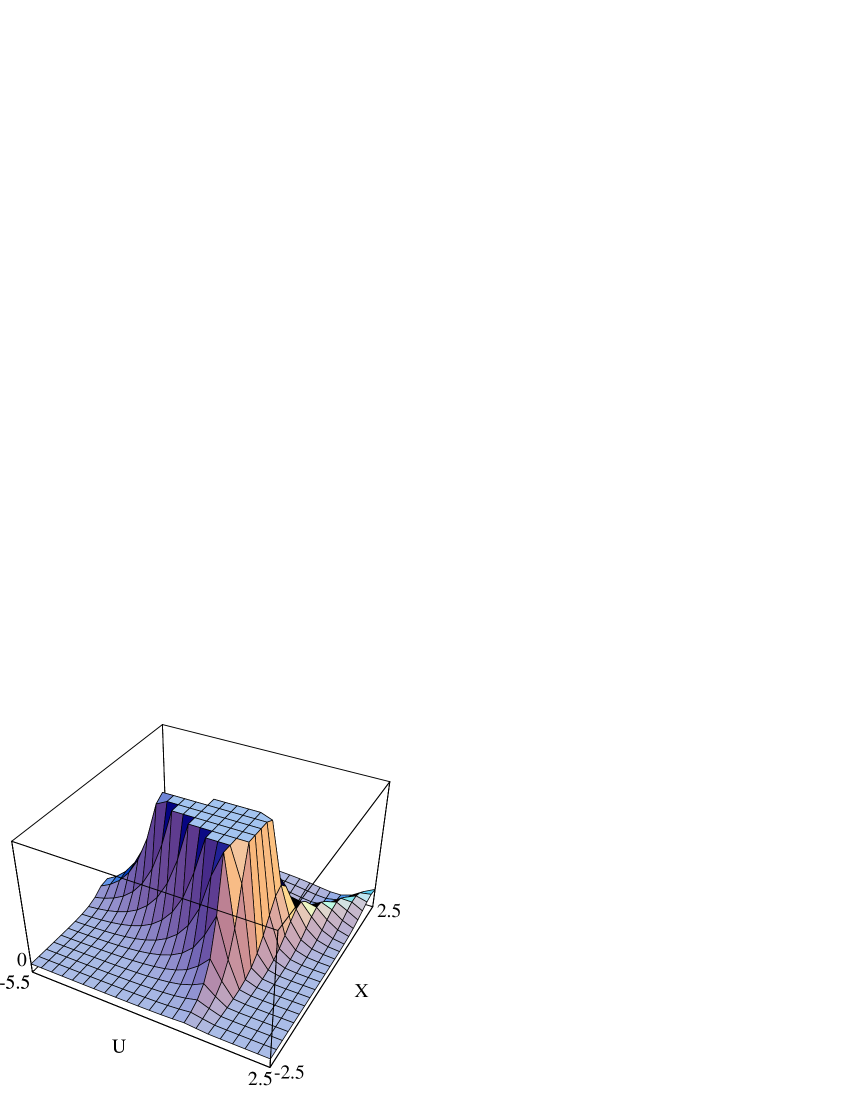
Figure 3: The typical form of the support of the ‘$V-A$’ two-point function. The upper $9/10$ of the figure is cripped.

The typical example of the support of the integration eq. (3.25) is shown in Fig. 3. This figure explicitly shows the cancellation of the ultraviolet divergences which results in the finiteness of the ‘V-A’ two-point function.

The QCD S parameter $S$ and the pion decay constant $f_{\pi}$ are evaluated from formulae (3.3).

$t_{F}$	0.3	0.5	0.7	0.9	1.1
$S$	0.432	0.464	0.478	0.481	0.470
$(f_{\pi}/\Lambda_{\rm QCD})^{2}\times 100$	3.43	4.05	4.10	3.75	3.12
$\Lambda_{\rm QCD}$ [MeV]	502	462	459	481	526

Table 1: $t_{F}$ dependence of the value of the QCD $S$ parameter and $f_{\pi}/\Lambda_{\rm QCD}$. We also show the values of $\Lambda_{\rm QCD}$ calculated by imposing $f_{\pi}=93$ MeV. We fix the lattice size as $N_{BS}=22$.

We show the values of $S$ and $f_{\pi}$ for several values of $t_{F}$ in Table. 1. We conclude that the QCD S parameter $S$ takes the value

$$S=0.43\sim 0.48~{},$$ (3.52)

in the improved ladder exact approximation. This value is 30% larger than the experimental value[13]. Our value (3.52) implies that the chirl symmetry is dynamically breaking in the improved ladder exact approximation. In addition, our value of $\Lambda_{\rm QCD}$ is consistent with the result from the homogeneous BS equation for the pion[6].

Next, we extract the mass $m_{\rho}$ and decay constant $f_{\rho}$ of the $\rho$ meson. The decay constant of the $\rho$ meson is defined by

$$\Bigl{\langle}{0}\Bigr{|}V_{\mu}^{a}(0)\Bigl{|}{\rho^{b}(q,\epsilon)}\Bigr{\rangle}=\delta^{ab}\epsilon_{\mu}f_{\rho}m_{\rho}~{}.$$ (3.53)

We use the $\chi^{2}$ method to extract these two values from the functional form of our two-point function $\Pi(q_{{}_{E}}^{2})\equiv\Pi_{VV}(q^{2})-\Pi_{AA}(q^{2})$. The $\chi^{2}$ is defined by

$$\chi^{2}=\sum_{q_{{}_{E}}^{2}}\left|\frac{\Pi(q_{{}_{E}}^{2})-F(q_{{}_{E}}^{2})}{\Pi(q_{{}_{E}}^{2})}\right|^{2}~{},$$ (3.54)

where $F(q_{{}_{E}}^{2})$ is a three-resonance form given by

$$F(q_{{}_{E}}^{2})=\frac{f_{\rho}^{2}m_{\rho}^{2}}{q_{{}_{E}}^{2}+m_{\rho}^{2}}-\frac{f_{{}_{R1}}^{2}m_{{}_{R1}}^{2}}{q_{{}_{E}}^{2}+m_{{}_{R1}}^{2}}+\frac{f_{{}_{R2}}^{2}m_{{}_{R2}}^{2}}{q_{{}_{E}}^{2}+m_{{}_{R2}}^{2}}~{}.$$ (3.55)

	Our value	Experiment
$f_{\rho}$ [MeV]	133	144 $\pm$ 8
$m_{\rho}$ [MeV]	643	770

Table 2: The best fitted values of the mass and decay constant of $\rho$ meson. We use our value of $\Lambda_{\rm QCD}$ ($=462$ [MeV]).

Minimizing $\chi^{2}$ by the six parameters in $F(q_{{}_{E}}^{2})$, we obtain the best fitted values of $f_{\rho}$ and $m_{\rho}$, which is shown in Table. 2. Our value of $m_{\rho}$ is free from the regularization of ultraviolet divergences because of the finiteness of the ‘V-A’ two-point function $\Pi(q_{{}_{E}}^{2})$. This point is superiour to the result in Ref. [24]. The masses and decay constants of the heavier mesons are unstable for fitting; we obtain several best fitting curves with different values of the masses and decay constants of the heavier mesons, although the best fitting curves seem to be almost the same. On the other hand, the lowest meson mass and decay constant are very stable.

Figure 4: Three pole fitting of our two-point function, $\Pi(q_{E}^{2})=\Pi_{VV}(q_{E}^{2})-\Pi_{AA}(q_{E}^{2})$. The solid line is the best fitting curve, the dots denote the value of our $\Pi(q_{E}^{2})$.

We find that the sum of the pole residues $f_{\rho}^{2}m_{\rho}^{2}-f_{R_{1}}^{2}m_{R_{1}}^{2}+f_{R_{2}}^{2}m_{R_{2}}^{2}$ vanishes, which implies that our $\Pi(q_{E}^{2})$ behaves as $1/q_{E}^{4}$ in the high energy region. This means that the spectral functions of our $\Pi(q_{E}^{2})$ satisfies the second Weinberg sum rule:

$$\int_{0}^{\infty}ds\left[\rho_{V}(s)-\rho_{A}(s)\right]=0~{}.$$ (3.56)

The result from the improved ladder approximation reproduces the high energy behavior of the ‘$V-A$’ two-point function required by that from Operator Product Expansion.

Part II Heavy Quark Symmetry and Isgur-Wise Function

4 The Determination of $|V_{\rm cb}|$

4.1 The Basic Notion of the Heavy Quark Effective Theory

The heavy quark effective theory (HQET) will give the most efficient method to treat the decay constants of the heavy mesons and the various form factors of the semi-leptonic heavy quark decay. The form factors are given by appropriate overlap integrals between the initial and final state wave functions of the heavy mesons.

The basic idea of the HQET is the following:

The heavy mesons such as $B$, $D$ and $D^{*}$ are the bound states formed by the strong interaction. The bound states consist of one heavy quark ($Q=b$ or $c$) and one light antiquark ($\overline{q}=\overline{u}$ or $\overline{d}$). This situation reminds us with the hydrogen atom in which the light electron is bounded around the heavy proton.

The masses of the heavy quarks are thought to be ideally infinity $M_{Q}=\infty$ in the HQET. We may expect that the $Q\overline{q}$ bound state by the strong interaction has the same properties as that the hydrogen atom has. Let us enumerate some of the important properties.

• The heavy quark behaves like ‘free particle’. Namely, the momentum recoil from the light antiquark, or we should say the light degree of freedom, is negligible compared with the mass of the heavy quark ($\Lambda_{\rm QCD}/M_{Q}=0$).

• From 1) the momentum of the heavy quark becomes a conserved quantity, and we are allowed to take the rest frame of the heavy quark as a Lorenz frame of the observer.

• From 2) the spin of the heavy quark becomes also a good quantum number, and the heavy spin symmetry $SU(2)_{HS}$ arises. The heavy flavor symmetry $SU(2)_{HF}$ emerges because the strong interaction does not distinguish the flavor of the heavy quarks $b$ and $c$. The symmetry group $SU(2)\times SU(2)$ enhances to $SU(4)$ like non-relativistic $SU(6)$ model of light quarks. Then the global symmetry $SU(2)_{f}$ which originally exists in the total system ($u$, $d$ are doublet and $b$, $c$ are singlet) extends to $SU(2)_{f}\times SU(4)_{HQ}$. The symmetry $SU(4)_{HQ}$ is called the heavy quark spin-flavor symmetry. In this case the heavy mesons $D$, $D^{*}$, $B$ and $B^{*}$ form the quartet of this symmetry.

• From 2) the BS amplitude $\chi=\langle 0|{\rm T}Q(x)\overline{q}(y)|X(q)\rangle$ which is the wave function of the heavy meson $X=D,D^{*},B,B^{*}$ factories into the heavy quark sector and the light quark sector:

  $$\chi=e^{-iqX}\Lambda_{+}\times\left[\begin{array}[]{c}\mbox{ the light quark sector which is described by }\\ \mbox{ only the light degrees of freedom in QCD }\end{array}\right]~{},$$

  where $X^{\mu}$ is the center-of-mass coordinate between $x^{\mu}$ and $y^{\mu}$ and $\Lambda_{+}=(1+v\kern-5.8pt\mbox{\it/})/2$ with $v_{\mu}=q_{\mu}/M_{B}$ is the projection operator which projects the heavy quark onto the positive energy.

Then, the form factors of the semi-leptonic $B$ decay given by overlap integrals of the wave functions factorize into the heavy quark sector and the sector of the light degrees of freedom. The heavy quark sector takes a simple form which represents that the ‘free’ $b$ quark decays to the ‘free’ $c$ quark though an appropriate weak current. The ‘free’ heavy quark means that she propagates without any recoils from the light degrees of freedom, and does not mean actual free quark. The light sector given by the overlap integral represents the transition from the cloud around the $b$ quark formed by the light degrees of freedom to the cloud around the $c$ quark.

It is very difficult to calculate these overlap integrals from the first principle. Fortunately, these overlap integrals are expressed in terms of a single universal function, so-called the Isgur-Wise function. When we consider the form factors of the transitions (decays) between the multiplets of the heavy quark spin-flavor symmetry, the marvelous theorem of Wigner-Eckert relates them to some universal scalar quantity up to the Clebsch-Gordan coefficients. Usually such universal scalar quantities are called reduced matrix element. The Isgur-Wise function is just the reduced matrix element:

$$\langle D^{*}(v^{\prime},\epsilon)|\overline{c}\gamma_{\mu}(1-\gamma_{5})b|B(v)\rangle = \left[(v^{\prime}\!\cdot\!v+1)\epsilon_{\mu}-(\epsilon\!\cdot\!v)v^{\prime}_{\mu}+i\varepsilon_{\mu\nu\rho\sigma}\epsilon^{\nu}v^{\prime}{}^{\rho}v^{\sigma}\right]\xi(v^{\prime}\!\cdot\!v)~{},$$

$$\langle D(v)|\overline{c}\gamma_{\mu}(1-\gamma_{5})b|B(v)\rangle = (v^{\prime}+v)_{\mu}\xi(v^{\prime}\!\cdot\!v)~{},$$

and so on where we adopt the mass independent normalization condition to the bound states $\langle B(v^{\prime})|B(v)\rangle=2v^{0}(2\pi)^{3}\delta^{3}({\mbox{\boldmath$q$}}-{\mbox{\boldmath$q$}}^{\prime})$.

The Isgur-Wise function is normalized absolutely at the kinematical end point. This fact is easily shown using the heavy quark spin-flavor symmetry and the non-renormalization theorem of the conserved current. The $B\rightarrow B$ matrix element of the $b$ quark current is given in terms of the Isgur-Wise function $\langle B(v^{\prime})|\overline{b}\gamma_{\mu}b|B(v)\rangle=(v^{\prime}+v)_{\mu}\,\xi(v^{\prime}\!\cdot\!v)$, while the conserved current $\overline{b}\gamma_{\mu}b$ receives no renormalization at the vanishing momentum transfer $v^{\prime}=v$. Thus, we find $\xi(1)=1$.

As for the leptonic decay of the heavy mesons, the corresponding reduced matrix element is $F_{B}\sqrt{M_{B}}$ where $F_{B}$ is the decay constant of the $B$ meson:

$$\begin{array}[]{ccccc}\langle 0|\overline{d}\gamma_{\mu}\gamma_{5}c|D(v)\rangle&=&\langle 0|\overline{u}\gamma_{\mu}\gamma_{5}b|B(v)\rangle&=&iF_{B}\sqrt{M_{B}}~{}v_{\mu}~{},\\ \langle 0|\overline{d}\gamma_{\mu}c|D^{*}(v,\epsilon)\rangle&=&\langle 0|\overline{u}\gamma_{\mu}b|B^{*}(v,\epsilon)\rangle&=&F_{B}\sqrt{M_{B}}~{}\epsilon_{\mu}~{}.\end{array}$$

Here we comment on the determination of the heavy meson decay constant. Usually the decay constant of a charged meson $M$ is determined from the combined lepton decay $M\rightarrow l\overline{\nu}+l\overline{\nu}\gamma$. In the case of heavy mesons, there is another way to extract the decay constant using the non-leptonic decays $B\rightarrow DD_{s}$ and $B\rightarrow D^{*}D_{s}$.[37] The decay constant $F_{D_{s}}$ is directly estimated from these processes using the factorization hypothesis. Decay constants of the other heavy mesons are calculated using the heavy quark symmetry.

Therefore, once we know some two matrix elements, such as $\xi(v^{\prime}\!\cdot\!v)$ and $F_{B}\sqrt{M_{B}}$, the other channels are completely determined using the heavy quark symmetry by virtue of the Wigner-Eckert theorem.

4.2 Experimental Point of View

The $\Upsilon(4S)$ resonance produces the $B^{0}\overline{B^{0}}$ or $B^{+}B^{-}$ pair. The $B$ mesons are produced almost in the laboratory frame because the invariant mass of those pairs are almost the same as the mass of the $\Upsilon(4S)$ resonance. The semi-leptonic decays of a $B$ meson which is one of those are used for the determination of $|V_{\rm cb}|$. Let us define the four-velocities of the $B$ and $D^{(*)}$ mesons as $v_{\mu}$ and $v_{\mu}{}^{\prime}$ respectively. Usually the kinematic variable is defined by $t=v^{\prime}\!\cdot\!v$ which is essentially the momentum transfer $(q-q^{\prime})^{2}$ to the lepton pair given by

$$t=\frac{M_{B}^{2}+M_{D^{(*)}}^{2}-(q-q^{\prime})^{2}}{2M_{B}M_{D^{(*)}}}~{}.$$ (4.1)

The momentum transfer has maximum value $(M_{B}-M_{D^{(*)}})^{2}$ at the zero recoil point and must be positive because the invariant mass of the lepton pair must be positive. Thus we have the kinematically allowed region

$$1\leq t\leq\frac{M_{B}^{2}+M_{D^{(*)}}^{2}}{2M_{B}M_{D^{(*)}}}\cong 1.5\sim 1.6~{}.$$ (4.2)

The differential decay rates are given by[42, 43]

$$\frac{d\Gamma(B\!\rightarrow\!Dl\overline{\nu})}{dt} = |V_{\rm cb}|^{2}\frac{G_{F}^{2}}{48\pi^{3}}(M_{B}\!+\!M_{D})^{2}M_{D}^{3}(t^{2}\!-\!1)^{3/2}\left|\xi_{+}(t)\!-\!\frac{M_{B}\!-\!M_{D}}{M_{B}\!+\!M_{D}}\xi_{-}(t)\right|^{2},$$

$$\frac{d\Gamma(B\!\rightarrow\!D^{*}l\overline{\nu})}{dt} = |V_{\rm cb}|^{2}\frac{G_{F}^{2}}{48\pi^{3}}(M_{B}\!-\!M_{D^{*}})^{2}M_{D^{*}}^{3}(t^{2}\!-\!1)^{1/2}F(t,\frac{M_{B}}{M_{D^{*}}})\Big{|}\xi_{A1}(t)\Big{|}^{2},$$

where $\xi_{\pm}(t)$, $\xi_{A1}(t)$ are the form factors and $F$ is a given function

$$F(t,x)=(t+1)^{2}\left[1+\frac{4t}{t+1}\frac{x^{2}-2tx+1}{(x-1)^{2}}\right]{}~{}.$$

We will give the definitions of the form factors $\xi_{\pm}(t)$ and $\xi_{A1}(t)$ later. The charged lepton is regarded as massless without any significant loss of accuracy. The helicities of the $D^{*}$ meson are summed over. Let us show the experimental results by the CLEO collaborations[44] in fig.5.

Figure 5: The product $|V_{\rm cb}|\xi_{A1}(t)$ as a function of $t$ in the CLEO data[44] where $y=t$ and $F=\xi_{A1}$. $|V_{\rm cb}|$ is extracted from the intercept by the extrapolation to $t=1$. The points are data for the decay rate of the decay $B\rightarrow D^{*}l\overline{\nu}$ divided by the factors other than $|V_{\rm cb}|\xi_{A1}(t)$ of eq. (LABEL:eq:_dif_decay_rates). The error bars are statistical only. The dotted lines indicate the contours for $1\sigma$ variations of the fit parameters. They use (a) a linear function and (b) a quadratic function for the extrapolation.

In the heavy quark effective theory the KM matrix element $|V_{\rm cb}|$ is determined at the kinematical end point, where the $B$ meson at rest decays into the $D$ or $D^{*}$ mesons at rest and the lepton and neutrino pair are emitted back to back. The kinematical end point is where the $D$ or $D^{*}$ meson receives no momentum recoil. It becomes possible in the heavy quark limit to determine the $|V_{\rm cb}|$ at the zero recoil point without any ambiguity stems from the functional form of the form factors by virtue of the heavy quark effective theory.

Moreover, the differential decay rate of $B\rightarrow D^{*}l\overline{\nu}$, not $B\rightarrow Dl\overline{\nu}$, is protected from $1/M_{Q}$ order corrections which break the heavy quark symmetry.[45, 46] So, the determined value of $|V_{\rm cb}|$ in the heavy quark limit is correct up to $1/M_{Q}$ order. We notice that the form factors which are protected from $1/M_{Q}$ corrections at the kinematical end point are just $\xi_{+}(t)$ and $\xi_{A1}(t)$, not $\xi_{-}(t)$. Then, the semi-leptonic decay $B\rightarrow D^{*}l\overline{\nu}$ is the best to extract $|V_{\rm cb}|$.[43]

However there are large statistical error at the zero recoil point. The zero recoil point (or kinematical end point) is actually the end point in phase space, and phase space volume is almost zero. The kinematical suppression factors such as $(t^{2}-1)^{3/2}$ and $(t^{2}-1)^{1/2}$ appear in eq. (LABEL:eq:_dif_decay_rates). The suppression for $B\rightarrow Dl\overline{\nu}$ is relatively stronger. We have thus relatively large statistical error because the number of events are suppressed at the zero recoil point.

In addition, there is more serious problem of an ambiguity related to the emission of the soft pion at the kinematical end point, which enhances the relative systematic error at that point. The $B$ meson decays to the standing $D$ or $D^{*}$ mesons. Successively, the $D^{*}$ meson also decays to the $D$ meson with the soft pion emitted:

$$\begin{array}[]{cc}\mbox{ decay channel }&\mbox{ branching ratio }\\ \hline\cr D^{*\pm}(2010)\rightarrow D^{0}(1865)\pi^{\pm}(140)&68\%\\ D^{*\pm}(2010)\rightarrow D^{\pm}(1869)\pi^{0}(135)&31\%\end{array}$$

The value of the mass difference between $D^{*}$ and $D$ is almost the same as that of the pion mass. Then, the emitted pion does not acquire the kinetic energy, and does not reach to the particle detectors. We note that the lifetimes of the pion are $\tau_{\pi^{\pm}}=7.8$ m and $\tau_{\pi^{0}}=25$ nm. The decay $D^{*}\rightarrow D^{\pm}\pi^{0}$ is more serious than $D^{*}\rightarrow D^{0}\pi^{\pm}$. As a result we become hard to distinguish which process occur, $B\rightarrow D^{*}$ or $B\rightarrow D$ at the zero recoil point. We have thus relatively large systematic error. The unexpected suppression of the differential decay rate in Fig.5 at the kinematical end point might stem from the above reason. Here we have a comment. As far as we believe the experimental data in Fig.5, it is seemed that the derivative of the form factor turns out to become positive around $t=y=1.15$, and is positive in the kinematical end point. This corresponds that the slope parameter $\rho^{2}$ of the Isgur-Wise function $\xi(t)$ becomes negative. The slope parameter is defined by

$$\rho^{2}=-\left.\frac{d\xi(t)}{dt}\right|_{t=1}~{}.$$

However it is shown by the QCD sum rule with a rigorous treatment[49, 50] that the slope parameter is bounded from below $\rho^{2}>1/4$ in the infinite heavy quark mass limit. Even though the actual data is not of the infinite heavy quark mass limit, we think that a contradiction exists.

4.3 Our Standpoint

Taking the experimental difficulties at the kinematical end point into account, therefore, in order to extract $|V_{\rm cb}|$ we are forced to extrapolate the value of the differential decay rate at the zero recoil point from the experimental data away from the point. How do we, however, know the functional form of the form factor? A linear and a quadratic functions are used in Ref.[44]. The parameters in the functions such as $\rho^{2}$ are determined from the experimental data by the $\chi^{2}$ fit.

There are several phenomenological models for the form factors. Some legitimate forms of the Isgur-Wise function are

$$\xi_{{}_{Linear}}(t) = 1-\rho^{2}(t-1)~{},$$

$$\xi_{{}_{BSW}}(t) = \frac{2}{t+1}\exp\left[\;-(2\rho^{2}-1)\frac{t-1}{t+1}\;\right]~{},$$

$$\xi_{{}_{ISGW}}(t) = \exp\left[\;-\rho^{2}(t-1)\;\right]~{},$$

$$\xi_{{}_{KS}}(t) = \left(\frac{2}{t+1}\right)^{2\rho^{2}}{}~{},$$ (4.4)

with the slope parameter $\rho^{2}$ as an free parameter. The first function is just a linear approximation. The second one is called the BSW model[51] and is derived from a relativistic oscillator model[52]. The third one is called the ISGW model[53] and is calculated from a valence quark model with the Coulomb and linear potential. The last one is called KS model[54] or the pole ansatz model. In Ref.[54] the exclusive semi-leptonic $B$ decays are studied in the spectator quark model. The helicity structure of the decays is matched to that of the semi-leptonic $b\!\rightarrow\!c$ ‘free’ quark decay at minimum momentum transfer $(q-q^{\prime})^{2}=0$. The $(q-q^{\prime})^{2}$ or $t$ dependence of the form factor is fixed by nearest one meson dominance in the $\overline{c}\gamma_{\mu}(1-\gamma_{5})b$ current channel, which produces a simple pole of the meson couples to that current. So, the slope parameter is given by $2\rho^{2}=1$ in the original literature.

Let us carry out the $\chi^{2}$ fitting to extract $|V_{\rm cb}|$ using the above four forms. The experimental result of CLEO[44] is used. The cited errors are only statistical, and the systematic errors are not included. We multiply the error bar at the kinematical end point by five just for convenience.

model	$|V_{\rm cb}|$	$\rho^{2}$	$\chi^{2}$
Linear	0.0362	0.866	0.846
BSW	0.0387	1.42	0.899
ISGW	0.0376	1.16	0.806
KS	0.0382	1.32	0.854

Table 3: The best fitted values of the KM matrix element $|V_{\rm cb}|$ and slope parameter $\rho^{2}$. These are determined from the experimental data of CLEO[44].

We give the value of the KM matrix element $|V_{\rm cb}|$, the slope parameter $\rho^{2}$ and $\chi^{2}$ extracted from the the experiment in Table 3. The $\chi^{2}$ is defined by

$$\chi^{2}=\sum_{i}\left|\frac{|V_{\rm cb}|\xi_{{}_{X}}(t_{i})-F_{i}}{\sigma_{i}}\right|^{2}~{},$$ (4.5)

where $X=Linear$, $BSW$, $ISGW$, $KS$ and $t_{i}$ is experimental data point, $F_{i}$ is experimental data of the combination $|V_{\rm cb}|\xi(t)$ at $t_{i}$ and $\sigma_{i}$ is relative error at $t_{i}$. It will be the best model that gives the least value of $\chi^{2}$ by tuning $|V_{\rm cb}|$ and $\rho^{2}$. The ISGW model gives the least $\chi^{2}$. The values of the KM matrix element $|V_{\rm cb}|$ and slope parameter $\rho^{2}$ deviate around 3% and 24% respectively. The determined values of $|V_{\rm cb}|$ are rather stable over these four models, but those of $\rho^{2}$ are not so stable. Square root of the slope parameter $\rho$ represents the size of the heavy mesons in unit of $\Lambda_{\rm QCD}$. The large value of $\rho^{2}$ means large size of the ‘cloud’ around the heavy quark in unit of the typical scale of binding energy and vice-versa. The size of the heavy meson becomes just input in the phenomenological models ignoring the strong interaction dynamics of the light degrees of freedom.

We would like to know the functional form of the form factor in more model independent way. For this purpose we need the detailed information of the wave function of the heavy mesons based on the dynamics of the strong interaction. Our main subject in Ref.[55] is to calculate the form factors in the heavy quark limit, i.e. the Isgur-Wise function, numerically from the Bethe-Salpeter amplitudes of the heavy mesons. The Isgur-Wise function is calculated as an overlap integral of the BS amplitudes of the heavy mesons.

The BS amplitudes are calculated from the BS equation for the pseudoscalar heavy meson with the three approximations i) constant mass, ii) improved ladder and iii) heavy quark limit ($M_{Q}\rightarrow\infty$). The first approximation is applied by replacing the mass functions of the heavy and light quarks with appropriate constants, i.e. some kind of a constituent mass. This replacement is just for the simplicity of the calculations. Ideally we should use the mass function with the same approximation ii), but we leave it in the future work. The typical values of the constant light quark mass is determined by the conditions $m=\Sigma(cm^{2})$ with $c=1,4$. The mass function $\Sigma(-p^{2})$ is calculated by the Schwinger-Dyson equation with the improved ladder approximation. As for the last one we adopt it to make good use of the basic idea (includes the heavy quark symmetry) implemented in the heavy quark effective theory.

5 Isgur-Wise Function from Bethe-Salpeter Amplitude

This section is devoted to the review of the literature in Ref.[55]. We show the basic formulations for the Bethe-Salpeter equation. We expand the BS equation in the inverse power of the heavy quark mass and keep only the leading order terms. The Isgur-Wise function is expressed by the overlap integral of the leading BS amplitudes. Finally we give the numerical results.

5.1 BS Amplitude for the $B$ Meson

We consider the bound state of the pseudoscalar heavy meson $|B(q)\rangle$. The bound state momentum is $q_{\mu}$ and its mass is $M_{B}$, so $q^{2}=M_{B}^{2}$. The bound state consists of the heavy quark $\Psi$ and the light anti-quark $\overline{\psi}$ with masses $M$ and $m$ respectively. The BS amplitude $\chi_{\alpha\beta}(p;q)$ of the bound state $|B(q)\rangle$ is defined by

$$\langle 0|{\rm T}\Psi_{\alpha i}(x)\overline{\psi}_{\beta}^{j}(y)|B(q)\rangle=e^{-iqX}\int\!\!\frac{d^{4}p}{(2\pi)^{4}i}~{}e^{-ipr}\delta_{i}^{j}~{}\chi_{\alpha\beta}(p;q)~{},$$ (5.1)

where $\alpha,\beta$ are spinor indices and $i,j$ are color indices. The Kronecker delta $\delta_{i}^{j}$ means that the bound state is color singlet. The center-of-mass coordinate $X^{\mu}$ and the relative coordinate $r^{\mu}$ are defined by

$$X^{\mu}=\zeta x^{\mu}+\eta y^{\mu}~{},\qquad r^{\mu}=x^{\mu}-y^{\mu}~{},$$ (5.2)

with weights

$$\zeta=\frac{M}{M+m}~{},\qquad\eta=\frac{m}{M+m}~{}.$$ (5.3)

Only the division with these weights (5.3) allow us to carry out the Wick rotation for any BS amplitudes.

The BS amplitude is decomposed into four invariant amplitudes $A$, $B$, $C$, $D$ as

$$\chi(p;q)=\sum_{i=1}^{2}\left[~{}\Gamma^{(+)}_{i}(p;v)\left(\begin{array}[]{c}A(p;q)\\ B(p;q)\end{array}\right)^{i}+\Gamma^{(-)}_{i}(p;v)\left(\begin{array}[]{c}C(p;q)\\ D(p;q)\end{array}\right)^{i}{}~{}\right]~{},$$ (5.4)

where $v_{\mu}=q_{\mu}/M_{B}$ is the four-velocity of the $B$ meson. The bispinor base $\Gamma^{(\pm)}_{i}(p;v)$ is defined by

$$\Gamma^{(\pm)}_{1}(p;v)=\Lambda_{\pm}\gamma_{5}~{},\qquad\Gamma^{(\pm)}_{2}(p;v)=\Lambda_{\pm}\mbox{\boldmath$p$}\kern-6.0pt\mbox{\it/}\gamma_{5}~{},$$ (5.5)

where ${\mbox{\boldmath$p$}}^{\mu}\equiv p^{\mu}-(p\!\cdot\!v)v^{\mu}$ and $\Lambda_{\pm}=(1\pm v\kern-5.8pt\mbox{\it/})/2$ is the projection operator. We note that the projection operators project an arbitrary state of the heavy quark onto a positive energy or negative energy amplitude and has the properties

$$\Lambda_{\pm}\Lambda_{\mp}=0~{},\qquad v\kern-5.8pt\mbox{\it/}\Lambda_{\pm}=\pm\Lambda_{\pm}~{},\qquad\Lambda_{\pm}\mbox{\boldmath$p$}\kern-6.0pt\mbox{\it/}\Lambda_{\pm}=0~{}.$$ (5.6)

The invariant amplitudes are scalar functions in $p^{2}$ and $p\cdot q$. It is convenient to introduce the real variables $u$ and $x$ by

$$p\!\cdot\!v=iu~{},\qquad p^{2}=-u^{2}-x^{2}~{},$$ (5.7)

when we carry out the Wick rotation on the BS amplitude. We mean that $u$ is the time component of $p^{\mu}$ and $x$ is the magnitude of the spatial component of $p^{\mu}$ in the rest frame for the $B$ meson $q^{\mu}=(M_{B},\vec{0})$. The invariant amplitude is a scalar function in $u$ and $x$; i.e. $X(p;q)=X(u,x)$ for $X=A,B,C,D$.

The conjugate BS amplitude $\overline{\chi}(p;q)$ of the bra-state $\langle B(q)|$ is defined by

$$\langle B(q)|{\rm T}\psi_{\beta j}(y)\overline{\Psi}_{\alpha}^{i}(x)|0\rangle=-e^{iqX}\int\!\!\frac{d^{4}p}{(2\pi)^{4}i}~{}e^{ipr}\delta^{i}_{j}~{}\overline{\chi}_{\beta\alpha}(p;q)$$ (5.8)

The conjugate BS amplitude is also decomposed into four invariant amplitudes $\overline{A}$, $\overline{B}$, $\overline{C}$, $\overline{D}$ as

$$\overline{\chi}(p;q)=\sum_{i=1}^{2}\left[~{}\overline{\Gamma}^{(+)}_{i}(p;v)\left(\begin{array}[]{c}\overline{A}(u,x)\\ \overline{B}(u,x)\end{array}\right)^{i}+\overline{\Gamma}^{(-)}_{i}(p;v)\left(\begin{array}[]{c}\overline{C}(u,x)\\ \overline{D}(u,x)\end{array}\right)^{i}{}~{}\right]~{},$$ (5.9)

where the conjugate bispinor base is defined by $\overline{\Gamma}^{(\pm)}_{i}(p;v)\equiv\gamma_{0}[\Gamma^{(\pm)}_{i}(p^{*};v)]^{\dagger}\gamma_{0}$. Once we know the BS amplitude $\chi$, its conjugate BS amplitude $\overline{\chi}$ is given by the relation

$$\overline{\chi}(p;q)=\gamma_{0}[\chi(p^{*};q)]^{\dagger}\gamma_{0}~{},$$ (5.10)

where performing the Wick rotations on $\chi$ and $\overline{\chi}$ is understood. This equality is found to hold provided that the mass $M_{B}$ of the bound state is real, using the BS equation for the conjugate amplitude. In the numerical calculation we actually encounter the complex value of $M_{B}$. This point will be explained later. Comparing eq. (5.9) with eq. (5.10), we have $\overline{X}(u,x)=X^{*}(-u,x)$ for $X=A,B,C,D$. Because imaginary number $i$ comes into $X$ solely in the combination with $iu$, we find the relation

$$X^{*}(-u,x)=X(u,x)~{},$$ (5.11)

for $X=A,B,C,D$.

The Bethe-Salpeter equation for the $B$ meson in the improved ladder approximation reads

$$T\chi(p;q)=K\chi(p;q)~{}.$$ (5.12)

The kinetic part $T$ and the BS kernel $K$ are defined by

$$T(p;q) = S_{H}(p+\zeta q)\otimes S_{L}(p-\eta q)~{},$$

$$K\chi(p;q) = \int\!\!\frac{d^{4}k}{(2\pi)^{4}i}\gamma^{\mu}\chi(k;q)\gamma^{\nu}D_{\mu\nu}(p,k)$$ (5.13)

with

$$D_{\mu\nu}(p,k)=C_{2}g^{2}(p,k)\frac{1}{l^{2}}\left(g_{\mu\nu}-\frac{l_{\mu}l_{\nu}}{l^{2}}\right)\;~{},$$ (5.14)

where $l_{\mu}=(p-k)_{\mu}$, $C_{2}=(N_{c}^{2}-1)/(2N_{c})$ is the second Casimir invariant of color gauge group. The inverse propagators of the heavy and the light quarks are given in the constant mass approximation by

$$S_{H}(p+\zeta q) = p\kern-6.0pt\mbox{\it/}+\zeta q\kern-5.8pt\mbox{\it/}-M~{},$$

$$S_{L}(p-\eta q) = p\kern-6.0pt\mbox{\it/}-\eta q\kern-5.8pt\mbox{\it/}-m~{}.$$ (5.15)

As we show later the BS equation becomes an eigenvalue equation of the binding energy $E$ of the bound state and the BS amplitude in the heavy quark limit. The binding energy $E$ of the bound state is defined by

$$M_{B}=M+m-E=\zeta^{-1}(M-\zeta E)~{}.$$ (5.16)

For the development of the notation we introduce bra-ket notations

$$\chi(p;q)\longleftrightarrow|\chi\rangle\kern-3.5pt\rangle~{},\quad\overline{\chi}(p;q)\longleftrightarrow\langle\kern-3.5pt\langle\chi|~{},$$ (5.17)

$$A\chi(p;q)B\longleftrightarrow A\otimes B|\chi\rangle\kern-3.5pt\rangle~{},\quad\displaystyle\int\!\!\frac{d^{4}k}{(2\pi)^{4}i}~{}K(p,k)\chi(k;q)\longleftrightarrow K|\chi\rangle\kern-3.5pt\rangle~{},$$ (5.18)

It is convenient to introduce a inner product:

$$\langle\kern-3.5pt\langle\psi|\chi\rangle\kern-3.5pt\rangle=N_{c}\int\!\!\frac{d^{4}p}{(2\pi)^{4}i}{\rm tr}\big{[}\,\overline{\psi}(p;q)\chi(p;q)\,\big{]}~{}.$$ (5.19)

Then, the BS equation (5.12) is rewritten by the simple form:

$$T|\chi\rangle\kern-3.5pt\rangle=K|\chi\rangle\kern-3.5pt\rangle~{}.$$ (5.20)

In the heavy quark system it is useful to adopt the following normalization to the bound state:

$$\langle B(q)|B(q^{\prime})\rangle=2v^{0}(2\pi)^{3}\delta^{3}({\mbox{\boldmath$q$}}-{\mbox{\boldmath$q$}}^{\prime})~{},$$ (5.21)

where $v_{\mu}=q_{\mu}/M_{B}$. We call this the mass independent normalization. It is convenient to introduce the quantity

$$\rho\equiv v^{\mu}\frac{\partial T}{\partial q^{\mu}}=\zeta v\kern-5.8pt\mbox{\it/}\otimes S_{L}-\eta S_{H}\otimes v\kern-5.8pt\mbox{\it/}{}~{}.$$ (5.22)

The normalization condition for the BS amplitude is given by the Mandelstam formula, which reads

$$\langle\kern-3.5pt\langle\chi|\rho|\chi\rangle\kern-3.5pt\rangle=2~{}.$$ (5.23)

When we obtain the normalized BS amplitude, we can immediately calculate the decay constant of the $B$ meson. The decay constant of the $B$ meson is defined by

$$iv_{\mu}\,F_{B}\sqrt{M_{B}}=\langle 0|\overline{\Psi}\gamma_{\mu}\gamma_{5}\psi(0)|B(q)\rangle~{},$$ (5.24)

where the factor $\sqrt{M_{B}}$ comes from our definition of the state normalization (5.21). Multiplying eq. (5.24) by $v^{\mu}$ and substituting the BS amplitude $\chi$ into eq. (5.24), we have

$$F_{B}\sqrt{M_{B}}=-N_{c}\int\!\!\frac{d^{4}p}{(2\pi)^{4}i}{\rm tr}\Big{[}v\kern-5.8pt\mbox{\it/}\gamma_{5}\chi(p;q)\Big{]}~{}.$$ (5.25)

For the numerical calculation it is rewritten in terms of the invariant amplitudes as

$$F_{B}\sqrt{M_{B}}=N_{c}\int\frac{x^{2}dxdu}{2\pi^{3}}[A(u,x)-C(u,x)]~{}.$$ (5.26)

The decay constant of the $B$ meson is measured from the leptonic decay induced by the non-conserving weak current $\overline{u}\gamma_{\mu}b$ (with ambiguous CKM mixing matrix element $V_{\rm ub}$). The conservation of this current is violated only by the mass of the heavy quark, so there is no ultraviolet divergence to cause the renormalization of the current. The current receives only a finite renormalization because it is a dimensionful parameter that violates current conservation. The decay constant is calculated using a ultraviolet cutoff in our calculation. Then, the decay constant of the $B$ meson is regarded as the quantity in such cutoff scale, although it has no ultraviolet divergence. However, the resulting decay constant is directly connected with the real observable because it has no dependence of renormalization point, and is the on-shell quantity (of the $B$ meson).

In the full theory the renormalization constant of the current is indeed finite and depends on the heavy quark masses by a logarithmic correction. When we take the heavy quark limit such ‘finite’ renormalization constant may diverges. In the heavy quark effective theory where the heavy quark limit is taken for the first time, the current needs renormalization of the ultraviolet divergence because the theory is defined in the low energy limit much lower than the scale of the heavy quark masses, and the current depends on the renormalization point.[30, 31, 32] Some of the two-point functions, say $\langle 0|T\overline{u}\gamma_{\mu}b(x)\overline{u}\gamma_{\mu}b(0)|0\rangle$ has divergence because it is calculated on the vacuum using the inhomogeneous BS equation. This divergence is not of the current itself.

In the homogeneous BS formulation (with ladder diagrams), however, it needs no renormalization at all likewise the full theory defined by some kind of mass-dependent renormalization scheme[33] where the threshold effect is naturally built in. Any quantities, as well as the current $\overline{u}\gamma_{\mu}b$, which are defined on the non-perturbative bound states, not the vacuum, have no divergences. We introduce a ultraviolet cutoff to define the system for calculations, but it is just a convention for the calculations.

5.2 Heavy Quark Mass Expansion

Now, we expand all quantities in terms of the parameter $m/M$. The light quark mass $m$ appearing in the expansion parameter is just for the convenience to make dimension-less parameter. In this sense we are allowed to use $\Lambda_{\rm QCD}$ in stead of $m$. The important point is that we should expand in the inverse power of the heavy quark mass $M$.

The binding energy and BS amplitude are expanded as

$$\zeta E = E_{0}+\bigg{(}\frac{m}{M}\bigg{)}E_{1}+\bigg{(}\frac{m}{M}\bigg{)}^{2}E_{2}+\cdots~{},$$

$$\chi = \chi_{0}+\bigg{(}\frac{m}{M}\bigg{)}\chi_{1}+\bigg{(}\frac{m}{M}\bigg{)}^{2}\chi_{2}+\cdots~{}.$$ (5.27)

The expansion of the BS amplitude begins with the zeroth order in $m/M$ because of the mass independent normalization eq. (5.23). Even when we do not use such normalization condition, the difference of the two cases is absorbed in the overall constant of amplitudes. The expansion of the binding energy also begins with the zeroth order. We think that the binding energy of the first few lowest-lying states are of the order of the typical scale in the strong interaction. Then, we regard it as the order one $O(1)$ quantity. Although the binding energy depends on the heavy quark mass in general, the dependence is of the sub-leading order in $O(1)$.

Expanding the quark inverse propagators, we find

$$\begin{array}[]{ccl}S_{H}&=&\displaystyle\bigg{(}\frac{m}{M}\bigg{)}^{-1}S_{H-}+S_{H0}+\bigg{(}\frac{m}{M}\bigg{)}S_{H1}+\cdots~{},\vskip 6.0pt plus 2.0pt minus 2.0pt\\ S_{H-}&\equiv&-m(1-v\kern-5.8pt\mbox{\it/})=-2m\Lambda_{-}~{},\vskip 6.0pt plus 2.0pt minus 2.0pt\\ S_{H0}&\equiv&p\kern-6.0pt\mbox{\it/}-E_{0}v\kern-5.8pt\mbox{\it/}~{},\vskip 6.0pt plus 2.0pt minus 2.0pt\\ S_{H1}&\equiv&-E_{1}v\kern-5.8pt\mbox{\it/}~{},\vskip 6.0pt plus 2.0pt minus 2.0pt\\ \vdots&&\qquad\vdots\end{array}$$ (5.28)

and

$$\begin{array}[]{ccl}S_{L}&=&\displaystyle S_{L0}+\bigg{(}\frac{m}{M}\bigg{)}S_{L1}+\bigg{(}\frac{m}{M}\bigg{)}^{2}S_{L2}+\cdots~{},\vskip 6.0pt plus 2.0pt minus 2.0pt\\ S_{L0}&\equiv&p\kern-6.0pt\mbox{\it/}-m(1+v\kern-5.8pt\mbox{\it/})=p\kern-6.0pt\mbox{\it/}-2m\Lambda_{+}~{},\vskip 6.0pt plus 2.0pt minus 2.0pt\\ S_{L1}&\equiv&E_{0}v\kern-5.8pt\mbox{\it/}~{},\vskip 6.0pt plus 2.0pt minus 2.0pt\\ S_{L2}&\equiv&E_{1}v\kern-5.8pt\mbox{\it/}~{}.\vskip 6.0pt plus 2.0pt minus 2.0pt\\ \vdots&&\qquad\vdots\end{array}$$ (5.29)

Then, the kinetic part $T$ is expanded by

$$\begin{array}[]{ccl}T&=&\displaystyle\bigg{(}\frac{m}{M}\bigg{)}^{-1}T^{(-1)}+T^{(0)}+\bigg{(}\frac{m}{M}\bigg{)}T^{(1)}+\cdots~{},\vskip 6.0pt plus 2.0pt minus 2.0pt\\ T^{(-1)}&\equiv&S_{H-}\otimes S_{L0}~{},\vskip 6.0pt plus 2.0pt minus 2.0pt\\ T^{(0)}&\equiv&S_{H-}\otimes S_{L1}+S_{H0}\otimes S_{L0}~{},\vskip 6.0pt plus 2.0pt minus 2.0pt\\ T^{(1)}&\equiv&S_{H-}\otimes S_{L2}+S_{H0}\otimes S_{L1}+S_{H1}\otimes S_{L0}~{}.\vskip 6.0pt plus 2.0pt minus 2.0pt\\ \vdots&&\qquad\vdots\end{array}$$ (5.30)

We expand the quantity $\rho$ defined in eq. (5.22) as

$$\begin{array}[]{ccl}\rho&=&\displaystyle\rho^{(0)}+\bigg{(}\frac{m}{M}\bigg{)}\rho^{(1)}+\cdots~{},\vskip 6.0pt plus 2.0pt minus 2.0pt\\ \rho_{0}&\equiv&v\kern-5.8pt\mbox{\it/}\otimes S_{L0}-S_{H-}\otimes v\kern-5.8pt\mbox{\it/}~{},\vskip 6.0pt plus 2.0pt minus 2.0pt\\ &=&v\kern-5.8pt\mbox{\it/}\otimes(p\kern-6.0pt\mbox{\it/}-2m\Lambda_{+})+2m\Lambda_{-}\otimes v\kern-5.8pt\mbox{\it/}~{},\vskip 6.0pt plus 2.0pt minus 2.0pt\\ \rho_{1}&\equiv&v\kern-5.8pt\mbox{\it/}\otimes(S_{L1}-S_{L0})-(S_{H0}-S_{H-})\otimes v\kern-5.8pt\mbox{\it/}~{},\vskip 6.0pt plus 2.0pt minus 2.0pt\\ &=&2E_{0}v\kern-5.8pt\mbox{\it/}\times v\kern-5.8pt\mbox{\it/}-v\kern-5.8pt\mbox{\it/}\otimes(p\kern-6.0pt\mbox{\it/}-2m\Lambda_{+})-(p\kern-6.0pt\mbox{\it/}+2m\Lambda_{-})\otimes v\kern-5.8pt\mbox{\it/}~{},\vskip 6.0pt plus 2.0pt minus 2.0pt\\ \vdots&&\qquad\vdots\end{array}$$ (5.31)

The BS kernel $K$ is of order one quantity because it does not depend on the heavy quark mass $M$. Substituting all the above expansions into the BS equation eq. (5.12) or eq. (5.20), we have equalities order by order in $m/M$:

$$\begin{array}[]{ccl}\displaystyle\bigg{(}\frac{m}{M}\bigg{)}^{-1}&:&T^{(-1)}\chi_{0}=0~{},\vskip 6.0pt plus 2.0pt minus 2.0pt\\ \displaystyle\bigg{(}\frac{m}{M}\bigg{)}^{0}&:&\displaystyle T^{(-1)}\chi_{1}+T^{(0)}\chi_{0}=K\chi_{0}~{},\vskip 6.0pt plus 2.0pt minus 2.0pt\\ \displaystyle\bigg{(}\frac{m}{M}\bigg{)}^{1}&:&\displaystyle T^{(-1)}\chi_{2}+T^{(0)}\chi_{1}+T^{(1)}\chi_{0}=K\chi_{1}~{},\vskip 6.0pt plus 2.0pt minus 2.0pt\\ \vdots&&\qquad\vdots\end{array}$$ (5.32)

We solve the set of the BS equation (5.32) in the descending way. The most important parts are of order $O(m/M)^{-1}$ and $O(m/M)^{0}$. In the heavy quark limit only these two parts survive and describe the light degrees of freedom.

5.3 Heavy Quark Spin-Flavor Symmetry

Since $S_{H-}\propto\Lambda_{-}$ and $S_{L0}$ is invertible, the -1st order equation (5.32) reads

$$\Lambda_{-}\chi_{0}=0~{}.$$ (5.33)

We call this the positive energy condition. This condition implies

$$\chi_{0}=\Lambda_{+}\chi_{0}~{}.$$ (5.34)

This means that the leading BS amplitude $\chi_{0}$ involve no negative energy state of the heavy quark. Hence $\chi_{0}$ is decomposed into two invariant amplitudes $A,B$ appearing in eq. (5.4).

When we project the zeroth order BS equation (5.32) onto the positive energy states, we have

$$\Lambda_{+}T^{(0)}\chi_{0}=\Lambda_{+}K\chi_{0}~{},$$

where we use $\Lambda_{+}T^{(-1)}=0$. Using eq. (5.34), the explicit form of $T^{(0)}$ in eq. (5.30) and $\Lambda_{+}\gamma^{\mu}\Lambda_{+}=v^{\mu}\Lambda_{+}$, we finally obtain

$$(p\!\cdot\!v-E_{0})\chi_{0}(p\kern-6.0pt\mbox{\it/}-2m\Lambda_{+})=K_{0}\chi_{0}~{},$$ (5.35)

where we define the kernel $K_{0}$ as

$$K_{0}\chi=\int v^{\mu}\chi\gamma^{\nu}D_{\mu\nu}~{}.$$ (5.36)

This is the leading BS equation for the $B$ meson.

Now, we show that the leading BS equation has so-called the heavy quark spin-flavor symmetry. We can easily see that the equation possesses the heavy flavor symmetry because it includes no heavy quark mass. The heavy spin symmetry[28] is also shown to be exist from a fact. The multiplication from the left by any $2\times 2$ matrix remains invariant the leading BS equation (5.35). We consider the case where those matrices have inverses. The positive energy condition (5.33) should be kept, and all matrices which commute with the projection operator $\Lambda_{-}$ generate the symmetry of the system. In other words, the transformations which keep the positive energy condition forms a group. This group is found to be the spin rotation symmetry $SU(2)$ of the heavy quark.[55]

Let us show that the pseudoscalar and vector meson form doublet of the spin symmetry. As stated above the leading order BS amplitude for the pseudoscalar meson has two invariant amplitudes:

$$\chi_{0P}=\Lambda_{+}\gamma_{5}(A_{P}-B_{P}\mbox{\boldmath$p$}\kern-6.0pt\mbox{\it/})~{}.$$ (5.37)

While, the BS amplitude for the vector meson has eight invariant amplitudes:

$$\chi_{V}=\Lambda_{+}\left[\epsilon\kern-5.2pt\mbox{\it/}(A_{V}-B_{V}\mbox{\boldmath$p$}\kern-6.0pt\mbox{\it/})+\epsilon\!\cdot\!p(C_{V}-D_{V}\mbox{\boldmath$p$}\kern-6.0pt\mbox{\it/})\right]+\Lambda_{-}\left[\epsilon\kern-5.2pt\mbox{\it/}(A^{\prime}_{V}-B^{\prime}_{V}\mbox{\boldmath$p$}\kern-6.0pt\mbox{\it/})+\epsilon\!\cdot\!p(C^{\prime}_{V}-D^{\prime}_{V}\mbox{\boldmath$p$}\kern-6.0pt\mbox{\it/})\right]~{},$$ (5.38)

where $\epsilon_{\mu}$ is the polarization vector of the vector meson, which satisfies $\epsilon^{2}=-1$ and $\epsilon\!\cdot\!v=0$. The BS equation for the vector meson (as well as other type of mesons) is exactly the same form as that for the pseudoscalar meson in eq. (5.20). Then, the $-1$st order BS equation reads

$$\Lambda_{-}\chi_{0V}=0~{}.$$ (5.39)

This implies that $A^{\prime}_{V}$, $B^{\prime}_{V}$, $C^{\prime}_{V}$ and $D^{\prime}_{V}$ vanish for the leading BS amplitude. The leading BS amplitude $\chi_{0V}$ of the vector mesons also satisfies the leading BS equation in eq. (5.35). This equation for the vector meson can be derived from the pseudoscalar BS equation by virtue of the heavy quark spin-flavor symmetry. Let us explain this. When we multiply eq. (5.35) by $\epsilon\kern-5.2pt\mbox{\it/}\gamma_{5}$ which keeps the positive energy condition (5.33) from the left, the equation itself does not change, but the BS amplitude changes to be

$$\chi_{0P}=\Lambda_{+}\gamma_{5}(A_{P}-B_{P}\mbox{\boldmath$p$}\kern-6.0pt\mbox{\it/})\quad\stackrel{{\scriptstyle\textstyle\epsilon\kern-5.2pt\mbox{\it/}\gamma_{5}}}{{\longrightarrow}}\quad\Lambda_{+}\epsilon\kern-5.2pt\mbox{\it/}(A_{P}-B_{P}\mbox{\boldmath$p$}\kern-6.0pt\mbox{\it/}){}~{}.$$ (5.40)

The resulting BS equation is nothing but for the vector meson and determines the invariant amplitudes of the vector meson as

$$A_{V}=A_{P},\quad B_{V}=B_{P},\quad C_{V}=0,\quad D_{V}=0~{}.$$ (5.41)

Then, once we obtain the invariant amplitudes $A$, $B$ of, say, the pseudoscalar meson, we get both the pseudoscalar and vector BS amplitudes as

$$\chi_{0P} = \Lambda_{+}\gamma_{5}(A-B\mbox{\boldmath$p$}\kern-6.0pt\mbox{\it/})~{},$$

$$\chi_{0V} = \Lambda_{+}\epsilon\kern-5.2pt\mbox{\it/}(A-B\mbox{\boldmath$p$}\kern-6.0pt\mbox{\it/})~{}.$$ (5.42)

5.4 Isgur-Wise Function

It is enough to consider the matrix element $\langle B(v^{\prime})|\overline{b}\gamma_{\mu}b|B(v)\rangle$ of the elastic electromagnetic scattering of the pseudoscalar $B^{-}$ meson. The current conservation is expressed by

$$(v-v^{\prime})^{\mu}\langle B(v^{\prime})|\overline{b}\gamma_{\mu}b|B(v)\rangle=0~{}.$$ (5.43)

Then, the matrix element is described in terms of a single elastic form factor $f(t)$ as

$$\langle B(v^{\prime})|\overline{b}\gamma_{\mu}b|B(v)\rangle=(v+v^{\prime})_{\mu}~{}f(t){}~{},$$ (5.44)

where $t=v^{\prime}\!\cdot\!v$. The elastic form factor $f(t)$ approaches to the Isgur-Wise function in the heavy quark limit. When the matrix element is rewritten using the BS amplitude $\chi$ of the $B$ meson, its general form includes the current inserted five-point vertex function. Here we use the improved ladder approximation for the BS amplitude, while the current conservation eq. (5.43) should be incorporated. To satisfy this requirement we find[55]

$$\langle B(v^{\prime})|\overline{b}\gamma_{\mu}b|B(v)\rangle=N_{c}\int\!\!\frac{d^{4}p^{\prime}}{(2\pi)^{4}i}{\rm tr}\Big{[}\overline{\chi}(p^{\prime};q^{\prime})\gamma_{\mu}\chi(p;q)S_{L}(p^{\prime}\!-\!\eta q^{\prime}\!=\!p\!-\!\eta q)\Big{]}{}~{},$$ (5.45)

where the tree current $\gamma_{\mu}$ is used. We impose the condition $p^{\prime}\!-\!\eta q^{\prime}\!=\!p\!-\!\eta q$ which appears in the argument of the light quark propagator $S_{L}$. The momenta flowing in the light quark lines of the BS and conjugate BS amplitudes should be equal. We call this the momentum matching condition. We expand the both sides of eq. (5.45) in the inverse power of the heavy quark mass $M$. The leading term of the form factor $f(t)$ gives the Isgur-Wise function $\xi(t)$. Contracting the matrix element (5.45) with $(v+v^{\prime})^{\mu}$, we have

$$2(t+1)\xi(t)=N_{c}\int\!\!\frac{d^{4}p^{\prime}}{(2\pi)^{4}i}{\rm tr}\Big{[}\overline{\chi}_{0}(p^{\prime};q^{\prime})(v\kern-5.8pt\mbox{\it/}+v\kern-5.8pt\mbox{\it/}\,{}^{\prime})\chi_{0}(p;q)S_{L0}(p^{\prime}\!-\!mv^{\prime}\!=\!p\!-\!mv)\Big{]}~{}.$$ (5.46)

It is known that the Isgur-Wise function is absolutely normalized at the kinematical end point by

$$\xi(1)=1~{}.$$ (5.47)

This condition is satisfied in our formulation. At the point $t=1$ eq. (5.46) reduces to

$$2\xi(1)=N_{c}\int\!\!\frac{d^{4}p}{(2\pi)^{4}i}{\rm tr}\Big{[}\overline{\chi}_{0}(p;q)\,v\kern-5.8pt\mbox{\it/}\,\chi_{0}(p;q)S_{L0}\Big{]}~{}.$$ (5.48)

Whereas, the normalization condition of the leading BS amplitude is given from eq. (5.23) as

$$2=N_{c}\int\!\!\frac{d^{4}p}{(2\pi)^{4}i}{\rm tr}\Big{[}\overline{\chi}_{0}(p;q)\,v\kern-5.8pt\mbox{\it/}\,\chi_{0}(p;q)S_{L0}\Big{]}~{}.$$ (5.49)

The LHS of both equations (5.48) and (5.49) is exactly the same, then we have eq. (5.47). We recognize that the value of the Isgur-Wise function at the kinematical end point reduces exactly to the normalization of the leading BS amplitude.

In our formulation the Mandelstam normalization condition is rewritten by

$$\zeta\langle B(v)|\overline{b}\gamma_{\mu}b|B(v)\rangle-\eta\langle B(v)|\overline{u}\gamma_{\mu}u|B(v)\rangle=2v_{\mu}~{}.$$ (5.50)

Taking the derivative with $\zeta$ at the point (5.3), we have

$$\langle B(v)|\overline{b}\gamma_{\mu}b|B(v)\rangle+\langle B(v)|\overline{u}\gamma_{\mu}u|B(v)\rangle=0~{}.$$ (5.51)

Using both eqs. (5.50) and (5.51) we obtain

$$\langle B(v)|\overline{b}\gamma_{\mu}b|B(v)\rangle=-\langle B(v)|\overline{u}\gamma_{\mu}u|B(v)\rangle=2v_{\mu}~{}.$$ (5.52)

The equations (5.52) and (5.44) states that the Isgur-Wise function $\xi(t)$ and the elastic form factor $f(t)$ is absolutely normalized by the non-renormalization theorem of conserved current. We have shown that this mechanism is realized in our formulation. These interplay between the Mandelstam normalization condition and the current conservation tells us what Feynman diagram we should use to calculate the current matrix element.

The rest frame $v^{\prime}{}^{\mu}=(1,\vec{0})$ is used for the calculation of eq. (5.46). Then, the frame of the initial state is moving frame, and the four-velocity $v^{\mu}$ takes the form

$$v^{\mu}=(t,-\sqrt{t^{2}-1},0,0)~{}.$$ (5.53)

The integration variables $u^{\prime}$, $x^{\prime}$, $\cos\theta$ are the components of the relative momentum $p^{\prime}$, and are given by

$$p^{\prime}{}^{\mu}=(iu^{\prime},~{}x^{\prime}\cos\theta,~{}x^{\prime}\sin\theta\sin\varphi,~{}x^{\prime}\sin\theta\cos\varphi)~{},$$ (5.54)

where the angle $\varphi$ is trivially integrated to give the overall factor $2\pi$ because of the rotation symmetry in eq. (5.46), so we may put $\sin\varphi=1$ without loss of generality. Let us move to the $v^{\mu}$-rest frame, where we have

$$v^{\mu} = (1,~{}0,~{}0,~{}0)~{},$$

$$v^{\prime}{}^{\mu} = (t,~{}\sqrt{t^{2}-1},~{}0,~{}0)~{},$$

$$p^{\prime}{}^{\mu} = (iu^{\prime}t+x^{\prime}\cos\theta\sqrt{t^{2}-1},~{}x^{\prime}t\cos\theta+iu^{\prime}\sqrt{t^{2}-1},~{}x^{\prime}\sin\theta,~{}0)~{},$$

$$p^{\mu} = p^{\prime}{}^{\mu}-m(v^{\prime}-v)^{\mu}$$

$$= (iu^{\prime}t+x^{\prime}\cos\theta\sqrt{t^{2}-1}-m(t-1),~{}x^{\prime}t\cos\theta+(iu^{\prime}-m)\sqrt{t^{2}-1},~{}x^{\prime}\sin\theta,~{}0)~{}.$$

Thus, we find

$$u \equiv p\!\cdot\!v/i~{}~{}=~{}u^{\prime}t+i\Big{[}m(t-1)-x^{\prime}\cos\theta\sqrt{t^{2}-1}\Big{]}~{},$$

$$x \equiv \sqrt{\vec{p}\cdot\vec{p}}~{}=~{}\sqrt{\Big{[}x^{\prime}t\cos\theta+(iu^{\prime}-m)\sqrt{t^{2}-1}\Big{]}^{2}+\big{(}x^{\prime}\sin\theta\big{)}^{2}}~{}.$$ (5.56)

Let us rewrite eq. (5.46) into a component form. Substituting eq. (5.37) into eq. (5.46) and taking the trace over the spinor indices, we have

$$\xi(t)=\frac{N_{c}}{t+1}\int\frac{du^{\prime}x^{\prime}{}^{2}dx^{\prime}d\cos\theta}{8\pi^{3}}~{}\left(\begin{array}[]{c}A(u^{\prime},x^{\prime})\\ B(u^{\prime},x^{\prime})\end{array}\right)^{T}\left(\begin{array}[]{cc}L_{11}&L_{12}\\ L_{21}&L_{22}\end{array}\right)\left(\begin{array}[]{c}A(u,x)\\ B(u,x)\end{array}\right)~{},$$ (5.57)

with the momentum matching condition $p^{\prime}-mv^{\prime}=p-mv$. The $2\times 2$ matrix $L$ is defined by

$$L_{ij} \equiv \frac{1}{2}{\rm tr}\Big{[}\,\overline{\Gamma}_{i}(p^{\prime};v^{\prime})(v\kern-5.8pt\mbox{\it/}+v\kern-5.8pt\mbox{\it/}\,{}^{\prime})\Gamma_{j}(p;v)S_{L0}(p^{\prime}\!-\!\eta q^{\prime}\!=\!p\!-\!\eta q)\,\Big{]}~{},$$

$$L_{11} = iu^{\prime}(t+1)+k_{1}~{},$$

$$L_{12} = -(t+1)x^{2}-(t^{2}-1)iu(iu-m)-k_{1}^{2}+k_{1}\Big{(}(t+1)m-(2t+1)iu\Big{)}~{},$$

$$L_{21} = -(t+1)x^{2}-K_{1}(iu-2m)~{},$$

$$L_{22} = (t+1)\Big{(}iut-(t+1)m\Big{)}x^{2}+k_{1}^{2}(iu-2m)$$ (5.58)

$$\qquad\qquad+k_{1}\Big{[}tx^{2}-(t+1)(iu-m)(iu-2m)\Big{]}~{},$$

where $k_{1}=p^{\prime}\cdot(v-v^{\prime}t)=x^{\prime}\cos\theta\sqrt{t^{2}-1}$. At the kinematical end point, the matrix $L$ reduces to the weight matrix $\rho_{0}$:

$$L_{ij}\bigg{|}_{t=1}=2\rho_{0ij}(u^{\prime},x^{\prime})~{},$$ (5.59)

and as is stated the calculation of the Isgur-Wise function exactly gives unity, $\xi(1)=1$, by construction.

We should note that the variables $u$ and $x$ are complex, and we need the leading BS amplitudes $A(u,x)$ and $B(u,x)$ with the complex arguments. At the kinematical end point $t\!=\!1$, the variables $u$ and $x$ are real and identical to $u^{\prime}$ and $x^{\prime}$ respectively. In order to find the leading BS amplitude $(A(u,x),B(u,x))^{T}$ with complex arguments, we make use of the leading BS equation (5.5.3) itself:

$$\left(\begin{array}[]{c}A(u,x)\\ B(u,x)\end{array}\right)=\frac{\rho_{0}^{-1}(u,x)}{E_{0}-iu}\int\frac{y^{2}dydv}{8\pi^{3}}K_{0}(u,x;v,y)\left(\begin{array}[]{c}A(v,y)\\ B(v,y)\end{array}\right)~{},$$ (5.60)

We substitute values of $u$ and $x$ defined in eq. (5.56) into the RHS of eq. (5.60). We are already know the solution $E_{0}$ and $(A(v,y),B(v,y))^{T}$ for the ground state, then we also substitute this solution into the RHS of eq. (5.60). After carrying out the momentum integrations, we have the desired quantity $(A(u,x),B(u,x))^{T}$. We should notice that the above prescription to obtain the leading BS amplitude with complex arguments is not the analytic continuation of the leading BS amplitude with real arguments.

5.5 Numerical Calculation

5.5.1 Running Coupling

The running coupling in the one-loop approximation is given by

$$\alpha(\mu^{2})=\frac{g^{2}(\mu^{2})}{4\pi}=\frac{\alpha_{0}}{\ln\big{(}\mu^{2}/\Lambda_{\rm QCD}^{2}\big{)}}~{},$$ (5.61)

with

$$\alpha_{0}=\frac{12\pi}{33-2N_{f}}~{}.$$ (5.62)

The constant $\alpha_{0}$ depends on the number $N_{f}$ of quark flavors. The dominant part of the support of the leading BS amplitude lies below the threshold of $c$ quark, so we put $N_{f}=3$ and then $\alpha_{0}=4\pi/9$.

The running coupling (5.61) blows up at the $\Lambda_{\rm QCD}$ scale. For the numerical calculation we need the running coupling below the $\Lambda_{\rm QCD}$ scale, and we have to regularize it. We have no guidance on the form of the running coupling outside the deep Euclidean region $\mu^{2}\gg\Lambda_{\rm QCD}^{2}$. In what follows we rescale all dimensionful quantities by $\Lambda_{\rm QCD}$. The most simple prescription will be the Higashijima type:

$$\alpha(\mu^{2})=\frac{\alpha_{0}}{\ln\big{[}\max(\mu^{2},x_{0})\big{]}}~{},$$ (5.63)

with a constant $x_{0}$, but this violates analyticity. In order to calculate the Isgur-Wise function, the running coupling should be analytic within the integration region in eq. (5.60) needed to evaluate the leading BS amplitude with complex arguments.

For this purpose we adopt the following form:

$$\alpha(\mu^{2})=\frac{\alpha_{0}}{\ln f(\mu^{2})}~{},$$ (5.64)

with

$$f(x)=x+\kappa\ln\left[\,1+\exp\left(\frac{x_{0}-x}{\kappa}\right)\,\right]~{},$$ (5.65)

and use $\alpha(-p^{2}-k^{2})$ for the argument. The arbitrary constants $\kappa$ and $x_{0}$ are restricted to $\kappa>0$ and $x_{0}>1$. The function $f(x)$ approaches $x$ for large positive $x$, so that the asymptotic behavior of the running coupling is correct. The function $f(x)$ tends to a constant value $x_{0}$ for large negative $x$ or $x_{0}-x\ll\kappa$.

In order to describe the chiral symmetry breaking of the light degrees of freedom, the value of the running coupling in the infrared region should be large enough. We use the three values

$$x_{0}=1.01\,,\qquad 1.05\,,\qquad 1.10~{},$$ (5.66)

which correspond to $\alpha_{\max}=140.3$, $28.6$ and $14.6$ respectively.

Next we determine the constant $\kappa$. The function $f(x)$ has branch point singularities at

$$x_{s}\equiv x_{0}+i\pi\kappa(2n+1)~{},\qquad n\in{\bf Z}~{},$$ (5.67)

with the branch cuts extending along the real axis of $x$ to the left if we take the principal value of the logarithm. These singularities give rise to corresponding singularities in $\alpha(\mu^{2})$. If we take the limit $\kappa\rightarrow 0$, then the form of the running coupling reduces to the Higashijima type (5.63). But the singularity comes into the region needed to calculate the Isgur-Wise function. So, $\kappa$ must be sufficiently large. From the momentum matching condition, we have

$$-p^{2}=-p^{\prime}{}^{2}=2im(t-1)u^{\prime}-2mx^{\prime}\cos\theta\sqrt{t^{2}-1}+2m^{2}(t-1)~{}.$$ (5.68)

We can avoid the singularities in the function $f(-p^{2}-k^{2})$ if the imaginary part of $-p^{2}-k^{2}$ is lower than that of $x_{s}$;

$$|{\rm Im}(-p^{2}-k^{2})|=2m(t-1)u^{\prime}<\min(x_{s})~{},$$ (5.69)

in the case when the real part of $-p^{2}-k^{2}$ and $x_{s}$ are equivalent;

$${\rm Re}(x_{s}) = {\rm Re}(-p^{2}-k^{2})$$ (5.70)

$$= -k^{2}+u^{\prime}{}^{2}+\Big{(}\,x^{\prime}-m\cos\theta\sqrt{t^{2}-1}\,\Big{)}^{2}-m^{2}(t-1)\Big{(}(t+1)\cos\theta-2\Big{)}$$

$$\geq u^{\prime}{}^{2}-m^{2}(t-1)^{2}~{}.$$

In this case from eq. (5.70) $u^{\prime}$ is limited

$$u^{\prime}\leq u^{\prime}_{\max}=\sqrt{x_{0}+m^{2}(t-1)^{2}}~{}.$$ (5.71)

Thus, from eq. (5.69) we require

$$\kappa>\frac{2m(t-1)}{\pi}\sqrt{x_{0}+m^{2}(t-1)^{2}}~{},$$ (5.72)

for the range of the value of $t$ (4.2). This requirement (5.72) avoids all singularities and branch cuts stem from the running coupling.

5.5.2 Light Quark Mass $m$ and $\Lambda_{\rm QCD}$

It turns out that the leading order calculation need no particular value of the heavy quark mass $M$, but we have to fix the light quark mass $m$. There is no unique definition of the constituent quark mass. In our calculation the value of the light quark mass $m$ should be a typical value of the mass function $\Sigma(-p^{2})$ which is calculated from the Schwinger-Dyson equation with the improved ladder approximation in the chiral limit:

$$\Sigma(x)=\frac{3C_{2}}{4\pi}\int_{0}^{\infty}\!\!ydy\frac{\alpha(x+y)}{\max(x,y)}\;\frac{\Sigma(y)}{y+\Sigma(y)^{2}}~{}.$$ (5.73)

We work with the following two definitions:[56]

$$\begin{array}[]{lllll}m&=&\Sigma(m^{2})&&\mbox{ type I }~{},\\ m&=&\Sigma(4m^{2})&&\mbox{ type II }~{},\end{array}$$ (5.74)

where we call them type I mass and type II mass respectively.

In addition, we have to know the value of the unit scale $\Lambda_{\rm QCD}$ for the evaluation of the dimensionful observables such as $F_{B}$ and $E_{0}$. We notice that the Isgur-Wise function is dimension-less, and it requires no dimensionful scale unit. We calculate the pion decay constant $F_{\pi}(PS)$ using the obtained mass function $\Sigma(x)$ and the Pagels-Stokar formula[17] which reads

$$F_{\pi}(PS)^{2}=\frac{N_{c}}{2\pi^{2}}\int_{0}^{\infty}\!\!xdx~{}\frac{\Sigma(x)\Big{(}\Sigma(x)-x\Sigma^{\prime}(x)/2\Big{)}}{\big{(}x+\Sigma^{2}(x)\big{)}^{2}}~{}.$$ (5.75)

Imposing the value $F_{\pi}(PS)=93\sqrt{2}$ MeV allows us to fix $\Lambda_{\rm QCD}$.

As a consistency check of our choice of the running coupling form, we evaluate the vacuum expectation value of the quark bilinear $\langle 0|\overline{\psi}\psi|0\rangle_{\rm 1GeV}$ using the formula

$$\langle 0|\overline{\psi}\psi|0\rangle_{\rm 1GeV}=-\left(\frac{\alpha(\Lambda^{2})}{\alpha({\rm 1Ge^{2}})}\right)^{\frac{9C_{2}}{11N_{c}-2N_{f}}}\frac{N_{c}}{4\pi^{2}}\int_{0}^{\Lambda^{2}}\!\!xdx~{}\frac{\Sigma(x)}{x+\Sigma(x)^{2}}~{},$$ (5.76)

with $N_{f}=3$ and sufficiently large ultraviolet cutoff $\Lambda$. The calculated values are indeed consistent with the value given by Gasser and Leutwyler[57]

$$\langle 0|\overline{\psi}\psi|0\rangle_{\rm 1GeV}=-\big{(}225\pm 25{\rm MeV}\big{)}^{3}~{}.$$ (5.77)

$x_{0}$	$\Lambda_{\rm QCD}$	$m_{\rm typeI}$	$m_{\rm typeII}$	$\big{(}-\langle 0|\overline{\psi}\psi|0\rangle_{\rm 1GeV}\big{)}^{\frac{1}{3}}$
1.01	638	489	288	212
1.05	631	482	286	213
1.10	625	474	285	214

Table 4: Parameter values used in our calculation. Units are MeV.

We show all the results in Table 4.

5.5.3 BS Amplitude

Next, let us consider how we solve the leading BS equation (5.35). The notable property is that eq. (5.35) is an eigenvalue equation of the leading binding energy $E_{0}$ and leading BS amplitude $\chi_{0}$. In order to show this property more transparently we define the ‘Hamiltonian’ $H$ as

$$H=(p\!\cdot\!v)-\rho_{0}^{-1}K_{0}~{}.$$ (5.78)

Then, using $\chi_{0}(p\kern-6.0pt\mbox{\it/}-2m\Lambda_{+})=\rho_{0}\chi_{0}$, we have

$$E_{0}\,\chi_{0}=H\,\chi_{0}~{}.$$ (5.79)

For the purpose of the numerical calculation we rewrite the eigenvalue equation (5.79) into the component form. Multiplying by the conjugate bispinor base $\overline{\Gamma}_{i}^{(+)}$ and taking the trace we find

$$E_{0}\left(\begin{array}[]{c}A(u,x)\\ B(u,x)\end{array}\right)=iu\left(\begin{array}[]{c}A(u,x)\\ B(u,x)\end{array}\right)\\ +\rho_{0}^{-1}(u,x)\int\frac{y^{2}dydv}{8\pi^{3}}K_{0}(u,x;v,y)\left(\begin{array}[]{c}A(v,y)\\ B(v,y)\end{array}\right)~{},$$

where $\rho(u,x)$ and $K(u,x;v,y)$ are the $2\times 2$ matrices defined by

$$\rho_{0ij}(u,x) = \frac{1}{2}{\rm tr}\Big{[}\overline{\Gamma}_{i}^{(+)}(p;v)\rho_{0}\Gamma_{j}^{(+)}(p;v)\Big{]}$$ (5.82)

$$= \left(\begin{array}[]{cc}iu&-x^{2}\\ -x^{2}&x^{2}(iu-2m)\end{array}\right)~{},$$

and

$$K_{0ij}(u,x;v,y) = \int_{-1}^{1}\!\!d\cos\theta~{}\frac{1}{2}{\rm tr}\Big{[}\overline{\Gamma}_{i}^{(+)}(p;v)K_{0}(p;k)\Gamma_{j}^{(+)}(k;v)\Big{]}$$ (5.85)

$$= C_{2}g^{2}\left(\begin{array}[]{cc}I_{1}-(u-v)^{2}I_{2}&i(u-v)(y^{2}I_{2}-I_{2}^{\bf pk})\\ -i(u-v)(x^{2}I_{2}-I_{2}^{\bf pk})&I_{1}^{\bf pk}-(u-v)^{2}I_{2}^{\bf pk}\end{array}\right)~{}.$$

We define $\cos\theta$ by the angle between the three-vectors of the momentum $p^{\mu}$ and $k^{\mu}$ as

$$\cos\theta=\frac{\vec{p}\cdot\vec{k}}{|\vec{p}|\cdot|\vec{k}|}~{}.$$ (5.87)

The quantities $I_{1}$, $I_{2}$, $I_{1}^{\bf pk}$ and $I_{2}^{\bf pk}$ are defined by

$$\begin{array}[]{lclcl}I_{1}&=&\displaystyle\int_{-1}^{1}\!\!d\cos\theta~{}\frac{1}{-(p-k)^{2}}&=&\displaystyle\frac{1}{2xy}\ln\left(\frac{(x+y)^{2}+(u-v)^{2}}{(x-y)^{2}+(u-v)^{2}}\right)~{},\vskip 6.0pt plus 2.0pt minus 2.0pt\\ I_{2}&=&\displaystyle\int_{-1}^{1}\!\!d\cos\theta~{}\frac{1}{(p-k)^{4}}&=&\displaystyle\frac{2}{[(x+y)^{2}+(u-v)^{2}][(x-y)^{2}+(u-v)^{2}]}~{},\vskip 6.0pt plus 2.0pt minus 2.0pt\\ I_{1}^{\bf pk}&=&\displaystyle\int_{-1}^{1}\!\!d\cos\theta~{}\frac{{\mbox{\boldmath$p$}}\cdot{\mbox{\boldmath$k$}}}{-(p-k)^{2}}&=&\displaystyle\frac{x^{2}+y^{2}+(u-v)^{2}}{2}I_{1}-1~{},\vskip 6.0pt plus 2.0pt minus 2.0pt\\ I_{2}^{\bf pk}&=&\displaystyle\int_{-1}^{1}\!\!d\cos\theta~{}\frac{{\mbox{\boldmath$p$}}\cdot{\mbox{\boldmath$k$}}}{(p-k)^{4}}&=&\displaystyle\frac{x^{2}+y^{2}+(u-v)^{2}}{2}I_{2}-\frac{1}{2}I_{1}{}~{}.\end{array}$$ (5.88)

For further development of the numerical calculation, just for saving the memory in computers, first we restrict the integration region of the variable $v$ in eq. (5.5.3) to be positive by replacing the BS kernel part as

$$\int\!\!dvK_{0}(u,x;v,y)\left(\begin{array}[]{c}A(v,y)\\ B(v,y)\end{array}\right)\longrightarrow$$ (5.96)

$$\mathop{\int}_{v>0}\!\!dv\left[\,K_{0}(u,x;v,y)\left(\begin{array}[]{c}A(v,y)\\ B(v,y)\end{array}\right)+K_{0}(u,x;-v,y)\left(\begin{array}[]{c}A(-v,y)\\ B(-v,y)\end{array}\right)\,\right]~{}.$$

We divide the invariant amplitude $X(u,x)$ for $X=A$, $B$ into the even and odd part in $u$ as

$$X(u,x)\longrightarrow\left(\begin{array}[]{c}X_{e}(u,x)\\ X_{o}(u,x)\end{array}\right)\equiv\left(\begin{array}[]{c}X(u,x)+X(-u,x)\\ X(u,x)-X(-u,x)\end{array}\right)~{}.$$ (5.97)

When the invariant amplitude $X$ is of the real binding energy, this replacement corresponds to the division into the real and imaginary part because of eq. (5.11). Rewriting the leading BS equation (5.5.3) in terms of the even odd components $X_{e}$ and $X_{o}$ for $X=A$, $B$, we finally obtain

$$E_{0}\left(\begin{array}[]{c}A_{e}(u,x)\\ A_{o}(u,x)\\ B_{e}(u,x)\\ B_{o}(u,x)\end{array}\right) = \left(\begin{array}[]{cc|cc}0&-u&&\\ u&0&&\\ \hline\cr&&0&-u\\ &&u&0\end{array}\right)\left(\begin{array}[]{c}A_{e}(u,x)\\ A_{o}(u,x)\\ B_{e}(u,x)\\ B_{o}(u,x)\end{array}\right)+\rho_{0}^{-1}(u,x)\mathop{\int}_{v>0}\frac{y^{2}dydv}{8\pi^{3}}~{}$$ (5.110)

$$\times \left[\,{\cal K}_{0}(u,x;v,y)+{\cal K}_{0}(u,x;-v,y)\Sigma_{3}\,\right]\left(\begin{array}[]{c}A_{e}(v,y)\\ A_{o}(v,y)\\ B_{e}(v,y)\\ B_{o}(v,y)\end{array}\right){}~{}.$$ (5.115)

The weight matrix $\rho_{0}$ now becomes

$$\rho_{0}(u,x)=\left(\begin{array}[]{cc|cc}0&-u&-x^{2}&0\\ u&0&0&-x^{2}\\ \hline\cr-x^{2}&0&-2mx^{2}&-ux^{2}\\ 0&-x^{2}&ux^{2}&-2mx^{2}\end{array}\right)~{}.$$ (5.116)

The matrix $\Sigma_{3}$ is defined as

$$\left(\begin{array}[]{c}A_{e}(-v,y)\\ A_{o}(-v,y)\\ B_{e}(-v,y)\\ B_{o}(-v,y)\end{array}\right)=\left(\begin{array}[]{c}A_{e}(v,y)\\ -A_{o}(v,y)\\ B_{e}(v,y)\\ -B_{o}(v,y)\end{array}\right)=\Sigma_{3}\left(\begin{array}[]{c}A_{e}(v,y)\\ A_{o}(v,y)\\ B_{e}(v,y)\\ B_{o}(v,y)\end{array}\right)\longrightarrow\Sigma_{3}\equiv\left(\begin{array}[]{cc|cc}1&0&&\\ 0&-1&&\\ \hline\cr&&1&0\\ &&0&-1\end{array}\right){}~{}.$$ (5.117)

The quantity ${\cal K}_{0}(u,x;v,y)$ is the BS kernel $K_{0ij}(u,x;v,y)$ in eq. (LABEL:eq:_K0ij) extended to the $4\times 4$ matrix given by

$${\cal K}_{0}=\left(\begin{array}[]{cc|cc}K_{011}&0&0&-{\rm Im}K_{012}\\ 0&K_{011}&{\rm Im}K_{012}&0\\ \hline\cr 0&-{\rm Im}K_{021}&K_{022}&0\\ {\rm Im}K_{021}&0&0&K_{022}\end{array}\right)~{}.$$ (5.118)

The fundamental variables used to solve the leading BS equation numerically are $U$, $X$, $V$ and $Y$ defined by

$$u=\exp U,\quad x=\exp X,\quad v=\exp V,\quad y=\exp Y~{}.$$ (5.119)

We discretize these variables at $N_{BS}=30$ points evenly spaced in the intervals

$$U,V\in[\Lambda_{IRU},\Lambda_{UVU}]=[-10.0,2.5]~{},\quad X,Y\in[\Lambda_{IRX},\Lambda_{UVX}]=[-4.5,4.0]~{}.$$ (5.120)

Then, the integration appears in eq. (5.115) becomes the summation:

$$\mathop{\int}_{v>0}\!\!y^{2}dydv\qquad\longrightarrow\qquad DVDY\sum_{V,Y}VY^{3}~{},$$ (5.121)

with

$$DV=\frac{\Lambda_{UVU}-\Lambda_{IRU}}{N_{BS}-1}~{},\qquad DY=\frac{\Lambda_{UVX}-\Lambda_{IRX}}{N_{BS}-1}~{}.$$ (5.122)

The BS kernel ${\cal K}_{0}(u,x;v,y)$ in eq. (5.118) has an logarithmic integrable singularity at $(u,x)=(v,y)$, so we avoid it by the four-point average prescription given by

$${\cal K}_{0}(u,x;v,y)\quad\longrightarrow\frac{1}{4}\Big{[}{\cal K}_{0}(u,x;v_{+},y_{+})+{\cal K}_{0}(u,x;v_{+},y_{-})$$ (5.123)

$$+{\cal K}_{0}(u,x;v_{-},y_{+})+{\cal K}_{0}(u,x;v_{-},y_{-})\Big{]}~{},$$

with

$$v_{\pm}=\exp\left[V\pm\frac{1}{4}DV\right]~{},\qquad y_{\pm}=\exp\left[Y\pm\frac{1}{4}DY\right]~{}.$$ (5.124)

Now, we are in the position to solve the leading BS equation (5.115) as the eigenvalue equation numerically. We use FORTRAN subroutine package for the eigenvalue problem. The number of the point $N_{BS}$ is selected so that the discretisation dependences of the decay constant $F_{B}$ and the binding energy $E_{0}$ become small well within 1%. We chose the momentum region (5.120) so as for the supports of the integrand of the normalization condition (5.23) and decay constant (5.26) to be covered well enough. These supports extend much farther into the infrared region than in the case of the pion[6]. Consequently our results depend on the infrared behavior of the running coupling. We are therefore forced to regard $x_{0}$ as an input parameter in our approach.

When we numerically solve the leading BS equation, we throw away all abnormal solutions which have non-real eigenvalues, i.e. binding energies. We find the solution of the ground state; the largest binding energy and its corresponding eigenvector. This solution describes the lowest-lying quartet heavy mesons $B$, $B^{*}$, $D$ and $D^{*}$ of the heavy quark spin-flavor symmetry. The decay constant is easily calculated by eq. (5.26) with $C\!=\!0$.

type	$x_{0}$	m	$F_{B}\sqrt{M_{B}}$	$E_{0}^{(0)}$	$E_{0}^{(1)}$	$E_{0}^{(0)}-E_{0}^{(1)}$
I	1.01	489	2551	1795	1071	724
I	1.05	482	3468	935	498	437
I	1.10	474	4093	666	319	347
II	1.01	288	2052	1558	972	586
II	1.05	286	2738	799	447	352
II	1.10	285	3205	566	279	287

Table 5: $x_{0}$ dependence; $N_{\rm BS}=18$. Units are MeV except for $F_{B}\sqrt{M_{B}}$ which is in (MeV)^3/2.

The results of the binding energy and the decay constant using a coarser discretisation $N_{BS}\!=\!18$ is shown in Table 5. $E_{0}^{(0)}$ and $E_{0}^{(1)}$ are the binding energies of the ground and first excited states respectively. Ideally we would use the excitation energies $E_{0}^{(1)}\!-\!E_{0}^{(0)}$ to fix the parameter $x_{0}$ or the light quark mass $m$, but at present there is no experimental data for the masses of the radially excited pseudoscalar $B(1st)$, $D(1st)$ or vector $B^{*}(1st)$, $D^{*}(1st)$ mesons.

type	m	$F_{B(5279)}$	$F_{D(1869)}$	$B(\hbox{1st})-B(5279)$
I	482	48.0	80.6	432
II	286	37.8	63.4	350

Table 6: Results for the meson decay constants and mass difference with $N_{\rm BS}=30$ and $x_{0}=1.05$. $B(\hbox{1st})$ denotes first excited state of pseudoscalar $B$ meson. Units are MeV.

The $B$ and $D$ meson decay constants and mass differences using a finer discretisation $N_{BS}\!=\!30$ are given in Table 6. As can be seen, our result for $F_{B}$ is smaller than $F_{\pi}$, and is much smaller than other values obtained using QCD sum rules, potential models and lattice simulations (see tables in Ref.[37]). We note however that one gluon exchange interactions tend to give small values[38], even these are somewhat larger than our results.

The fact that the heavy meson decay constant is small means that the BS amplitude at the origin is suppressed, and the probability density leaks away from the origin so that the size of the heavy meson becomes large. We think that this fact is explained by our special prescription. We use the improved ladder approximation which does not realize the confining phenomena. In general the confining phenomena is realized by linear potential.[40, 41] However a special coupling choice of the improved ladder approximation enables us to realize the linear potential in a phenomenological way[39]. First, we impose two requirements such that asymptotic freedom and linear quark confinement be realized upon the non-relativistic quark potential $V(r)$. An simple interpolating form which invokes these requirements takes the form

$$V(r)=-\frac{4}{3}\int\!\!\frac{d^{3}{\mbox{\boldmath$p$}}}{(2\pi)^{3}}e^{-i{\mbox{\boldmath$p$}}\cdot\mbox{\boldmath$r$}}\frac{\alpha_{s}({\mbox{\boldmath$p$}}^{2})}{{\mbox{\boldmath$p$}}^{2}}~{},$$ (5.125)

with

$$\alpha_{s}({\mbox{\boldmath$p$}}^{2})=\frac{4\pi}{9}\frac{1}{\ln(1+{\mbox{\boldmath$p$}}^{2}/\Lambda^{2})}{}~{}.$$ (5.126)

Then if we use the form (5.126) in the improved ladder approximation, we will have confining force to tighten the size of the heavy meson.

Let us here comment on the occurrence of complex binding energies in our calculation. The leading BS equation reads

$$E_{0}\rho_{0}|\chi_{0}\rangle\kern-3.5pt\rangle={\cal A}|\chi_{0}\rangle\kern-3.5pt\rangle~{},$$ (5.127)

where ${\cal A}=\rho_{0}H$. Both quantities $\rho_{0}$ and ${\cal A}$ are hermitian in the norm defined by $(\chi^{\prime},\chi)\equiv\langle\kern-3.5pt\langle\chi^{\prime}|\rho_{0}|\chi\rangle\kern-3.5pt\rangle$. The special feature of the heavy quark system is that the natural norm which emerges from the leading BS equation (5.79) itself is exactly the same as of the Mandelstam formula in the heavy quark limit. It is not difficult to find the relation

$$(E_{0}-E^{\prime}_{0}{}^{*})\langle\kern-3.5pt\langle\chi^{\prime}|\rho_{0}|\chi\rangle\kern-3.5pt\rangle=0{}~{},$$ (5.128)

where $\chi^{\prime}$ and $\chi$ are the corresponding eigenvectors of the binding energies $E^{\prime}_{0}$ and $E_{0}$ respectively. Then, the binding energy is real otherwise the corresponding eigenvector has zero norm $\langle\kern-3.5pt\langle\chi|\rho_{0}|\chi\rangle\kern-3.5pt\rangle=0$. We actually encounter the non-real solutions for the binding energy and its corresponding null eigenvectors. These are abnormal solutions. We think that this is stemmed from the non-positivity of the weight matrix $\rho_{0}$. The sight violation of the hermiticity of ${\cal A}$ by the four-point splitting prescription will be not important. If the weight matrix $\rho_{0}$ would be positive definite matrix, the norm would be positive definite $\langle\kern-3.5pt\langle\chi|\rho_{0}|\chi\rangle\kern-3.5pt\rangle>0$. In this case we would never encounter the non-real solutions because of eq. (5.128). We note that the abnormal solution has zero eigenvalue for the charge of the conserved current $\overline{b}\gamma_{\mu}b$.

5.5.4 Isgur-Wise Function

The final form for the evaluation of the Isgur-Wise function needs five dimensional integrations. The $\cos\theta$ integration is evaluated using the Gauss-Legendre integration formula which gives rather precise results than interpolatory integration formulae. We save the discretisation point as $N_{GL}=10$.

Figure 6: Isgur-Wise functions calculated with $N_{BS}=30$, $N_{GL}=10$ and $x_{0}=1.05$ for both type I and type II masses.

We show our main result in Ref.[55] for the two types of light quark masses in Fig.6.

Figure 7: $x_{0}$ dependence of the Isgur-Wise function with type I mass, $N_{BS}=18$ and $N_{GL}=10$.

Figure 8: $x_{0}$ dependence of the Isgur-Wise function with type II mass, $N_{BS}=18$ and $N_{GL}=10$.

In Figs. 8 and 8 we show how the result depends on the parameter $x_{0}$, namely the low energy behavior of the running coupling for both the type I and type II masses. These data are evaluated from the leading BS amplitude with $N_{BS}=18$ points. We see that the result is almost independent of $x_{0}$ for the type I case, whereas there is some dependence for the type II case.

Some kind of fluctuations on our Isgur-Wise function are observed. The phenomena is explained in detail in Ref. [55]. We think that these fluctuations might stem from the violation of the analyticity of the leading BS amplitude. The momentum integrations $v$ and $y$ in eq. (5.60) cross over the branch cut of the quantity $I_{1}$ appears in the BS kernel $K_{0}(u,x;v,y)$. The quantity $I_{1}$ defined in eq. (5.88) has logarithmic singularity at the point $(v,y)=(u,x)$ and the branch extends from the point. We introduce the principal cut for the function $\ln(x)$.

The notable feature of our Isgur-Wise function is that the slope parameter $\rho^{2}$ is quite insensitive to the behavior of the running coupling in the low energy region as is shown in Figs. 8 and 8. The slope parameter slightly depends only on the value of the light quark mass. The values of the slope parameter $\rho^{2}$ for types I and II are as large as 2.0 and 1.8 respectively, which are somewhat larger than the known predictions. The estimated values of the slope parameter $\rho^{2}$ in literatures are given by $0.7\pm 0.2$[43], $1.0\sim 1.1$[58]

There is some controversy over the upper bound of the slope parameter. In Ref. [59] the upper bound is given by $\rho^{2}\leq 1.42$. Recently de Rafael and Taron[60] have argued that the form factor $F(q^{2})$ of the $B$ meson elastic scattering must satisfy the constraint

$$F_{-}(q^{2})<F(q^{2})<F_{+}(q^{2})~{},$$ (5.129)

where $F_{\pm}(q^{2})$ are given functions. As a result, they give a bound

$$\left.\frac{dF(q^{2})}{dq^{2}}\right|_{q^{2}=0}=\frac{1}{2(D-1)}\langle r^{2}\rangle\leq\frac{1}{16M_{B}^{2}}\left[D-\frac{5}{2}+\sqrt{\frac{2^{5}}{\pi C}-1}\right]~{},$$ (5.130)

where $D$ is the dimension of the spacetime and

$$C=\frac{15\sqrt{\pi}}{2^{D/2+4}N_{c}\Gamma\bigg{(}\displaystyle\frac{D+1}{2}\bigg{)}\Gamma\bigg{(}\frac{6-D}{2}\bigg{)}}~{}.$$ (5.131)

In Refs. [61, 62] they argue that it is impossible to obtain any such constrains at all when we carefully reconsider the heavy quark and light antiquark bound states lying below the heavy meson pair production threshold.

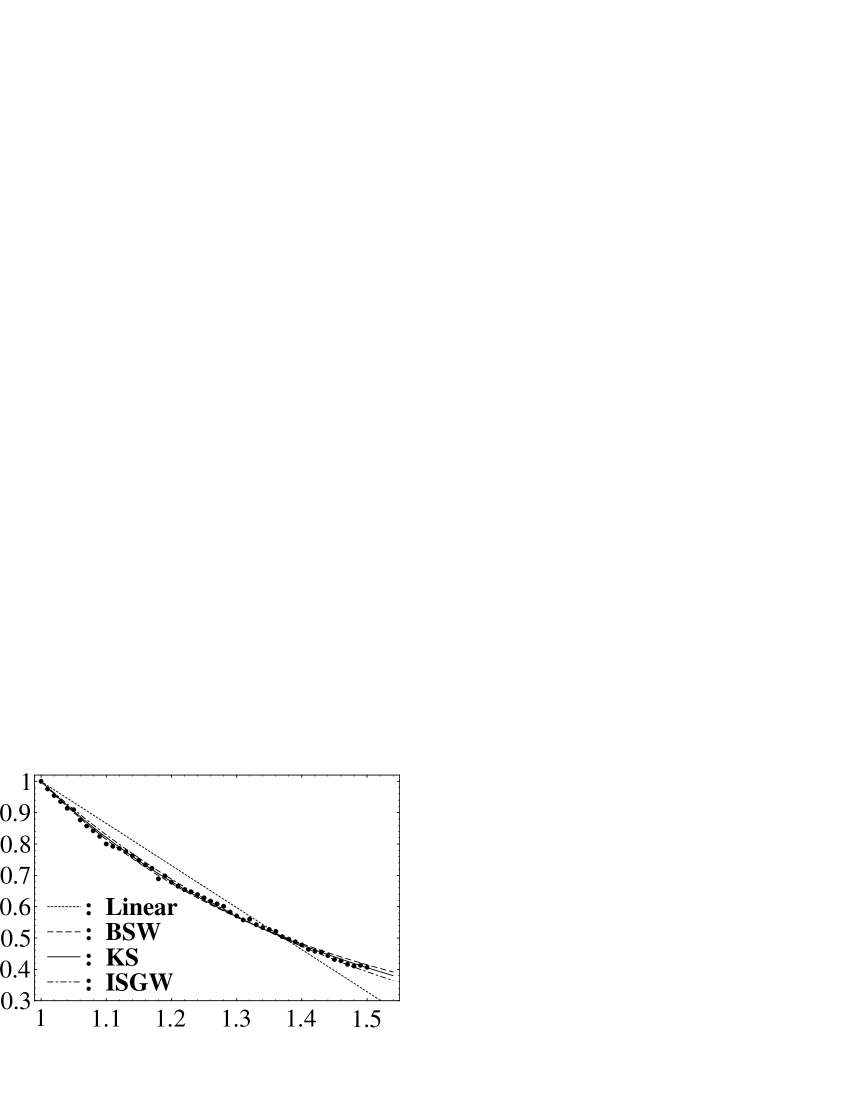
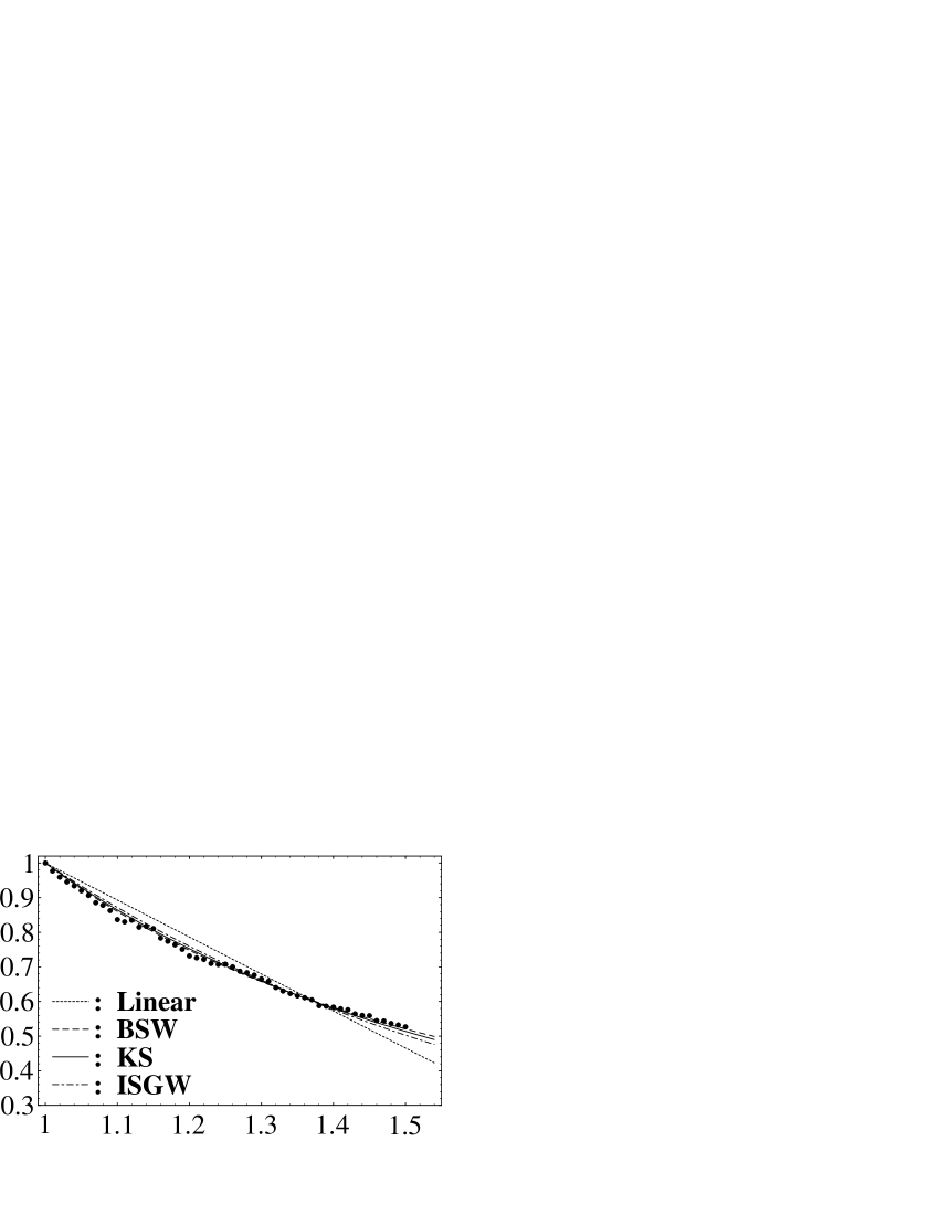
Figure 9: Phenomenological forms of the Isgur-Wise function. The slope parameters are extracted from our Isgur-Wise function in Fig. 6 with type I mass.

Figure 10: Phenomenological forms of the Isgur-Wise function. The slope parameters are extracted from our Isgur-Wise function in Fig. 6 with type II mass.

We use our Isgur-Wise function in Fig. 6 with type I and II masses to estimate the slope parameter $\rho^{2}$ in four phenomenological models by the $\chi^{2}$ fitting method as shown in Figs. 10 and 10.

type I
model	$\rho^{2}$	$\chi^{2}$
Linear	1.34	0.083
BSW	2.14	0.0038
ISGW	1.87	0.0055
KS	2.02	0.0028

type II
model	$\rho^{2}$	$\chi^{2}$
Linear	1.07	0.058
BSW	1.57	0.0033
ISGW	1.38	0.012
KS	1.49	0.0055

Table 7: The values of the slope parameter extracted from our Isgur-Wise function.

The values of the slope parameter are given in Table 7. The forms of the Isgur-Wise functions in the four models are given in eq. (4.4). The values of the slope parameter from our Isgur-Wise function with type I mass are relatively larger than from that with type II mass. KS and BSW models give the least $\chi^{2}$ for the type I and type II Isgur-Wise functions respectively. The other models except the linear form give also good fits.

Finally, we fit our Isgur-Wise function of Fig. 6 to the CLEO data by adjusting $|V_{\rm cb}|$ so as to minimize $\chi^{2}$.

Figure 11: $\xi(t)|V_{\rm cb}|$ versus $t$. Our Isgur-Wise functions in Fig. 6 are used for the determination of $|V_{\rm cb}|$.

The result is shown in Fig. 11. The experimental error bars in Fig. 11 are only statistical. The error bar at the kinematical end point is magnified five times, because of the systematic uncertainty stem from the soft pion emission. As is explained our Isgur-Wise function satisfies the condition $\xi(1)=1$ by construction. Thus, the intercept at $t=1$ gives $|V_{\rm cb}|$. We find the absolute values of the Kobayashi-Maskawa flavor mixing matrix element $|V_{\rm cb}|$ as

type $$|V_{\rm cb}|$$

I 0.0454 7.47

II 0.0401 0.979

(5.132)

The Isgur-Wise function with type II mass gives a better overall fit to the CLEO data as is seen from the value of $\chi^{2}$ in eq. (5.132). In other words, we are better to use the type II mass to describe the experiment.

6 Next-Leading Corrections of the Heavy-Light Quark Systems

In this section we consider the $1/M_{Q}$ next leading order corrections to the various form factors of the exclusive semi-leptonic $B\rightarrow D^{(*)}$ decays.

6.1 BS Amplitude

Let us first expand the normalization condition (5.23) in terms of $m/M$. Substituting eq. (5.31) into eq. (5.23), we have

$$2 = \langle\kern-3.5pt\langle\chi_{0}|\rho_{0}|\chi_{0}\rangle\kern-3.5pt\rangle$$ (6.1)

$$+ \bigg{(}\frac{m}{M}\bigg{)}\Bigg{\{}\langle\kern-3.5pt\langle\chi_{0}|\rho_{1}|\chi_{0}\rangle\kern-3.5pt\rangle+\langle\kern-3.5pt\langle\chi_{1}|\rho_{0}|\chi_{0}\rangle\kern-3.5pt\rangle+\langle\kern-3.5pt\langle\chi_{0}|\rho_{0}|\chi_{1}\rangle\kern-3.5pt\rangle\Bigg{\}}$$

$$+ O\bigg{(}\frac{m}{M}\bigg{)}^{2}~{}.$$

Thus, the normalization of the BS amplitude is determined order by order as

$$\begin{array}[]{ccl}\displaystyle\bigg{(}\frac{m}{M}\bigg{)}^{0}&:&2=\langle\kern-3.5pt\langle\chi_{0}|\rho_{0}|\chi_{0}\rangle\kern-3.5pt\rangle~{},\vskip 6.0pt plus 2.0pt minus 2.0pt\\ \displaystyle\bigg{(}\frac{m}{M}\bigg{)}^{1}&:&0=\langle\kern-3.5pt\langle\chi_{0}|\rho_{1}|\chi_{0}\rangle\kern-3.5pt\rangle+2{\rm Re}\langle\kern-3.5pt\langle\chi_{0}|\rho_{0}|\chi_{1}\rangle\kern-3.5pt\rangle~{},\vskip 6.0pt plus 2.0pt minus 2.0pt\\ \end{array}$$ (6.2)

where we use $\langle\kern-3.5pt\langle\chi_{1}|\rho_{0}|\chi_{0}\rangle\kern-3.5pt\rangle=\langle\kern-3.5pt\langle\chi_{0}|\rho_{0}|\chi_{1}\rangle\kern-3.5pt\rangle^{*}$. The leading order condition is previously used for the leading BS amplitude. The next-leading condition fixes the normalization of the next-leading amplitude $\chi_{1}$ in terms of the normalized leading BS amplitude. We notice that the total BS amplitude $\chi=\chi_{0}+(m/M)\chi_{1}+\cdots$ depends on the heavy quark mass although the next-leading BS amplitude $\chi_{1}$ does not depend on the heavy quark mass.

Next let us consider the BS equation in the next-leading order. Projecting the zeroth order BS equation (5.32) onto the negative energy states, we find

$$2m\Lambda_{-}\chi_{1}(p\kern-6.0pt\mbox{\it/}-2m\Lambda_{+})=\Lambda_{-}p\kern-6.0pt\mbox{\it/}\chi_{0}(p\kern-6.0pt\mbox{\it/}-2m\Lambda_{+})-\Lambda_{-}K\chi_{0}~{}.$$ (6.3)

This equation determines the negative energy part of the next-leading BS amplitude $\Lambda_{-}\chi_{1}$ from the leading BS amplitude $\chi_{0}$.

On the other hand, projecting the first order BS equation (5.32) onto the positive energy states, we obtain

$$\Lambda_{+}T^{(0)}\chi_{1}+\Lambda_{+}T^{(1)}\chi_{0}=\Lambda_{+}K\chi_{1}~{}.$$

This gives

$$(T_{0}-K_{0})\Lambda_{+}\chi_{1} = -E_{0}(p\!\cdot\!v-E_{0})\chi_{0}v\kern-5.8pt\mbox{\it/}+E_{1}\chi_{0}(p\kern-6.0pt\mbox{\it/}-2m\Lambda_{+})$$ (6.4)

$$+ \Lambda_{+}p\kern-6.0pt\mbox{\it/}\Lambda_{-}\chi_{1}(p\kern-6.0pt\mbox{\it/}-2m\Lambda_{+})+\Lambda_{+}K\Lambda_{-}\chi_{1}~{},$$

where we use $\chi_{1}=\Lambda_{+}\chi_{1}+\Lambda_{-}\chi_{1}$ and put

$$T_{0}\equiv(p\!\cdot\!v-E_{0})\otimes(p\kern-6.0pt\mbox{\it/}-2m\Lambda_{+})~{}.$$ (6.5)

This equation (6.4) gives the positive energy part of the next-leading BS amplitude $\Lambda_{+}\chi_{1}$ in terms of the leading BS amplitude $\chi_{0}$.

First, eq. (6.4) determines the next-leading binding energy $E_{1}$. Pre-multiplying eq. (6.4) by $\langle\kern-3.5pt\langle\chi_{0}|$, using $\langle\kern-3.5pt\langle\chi_{0}|(T_{0}\!-\!K_{0})=0$, eq. (6.2) and the non-renormalization theorem for the light quark current

$$\langle\kern-3.5pt\langle\chi_{0}|S_{H0}\otimes v\kern-5.8pt\mbox{\it/}|\chi_{0}\rangle\kern-3.5pt\rangle=-1~{},$$ (6.6)

we have

$$E_{1}=-E_{0}-\langle\kern-3.5pt\langle\chi_{0}|K|\Lambda_{-}\chi_{1}\rangle\kern-3.5pt\rangle~{}.$$ (6.7)

The light quark current $\overline{u}\gamma_{\mu}u$ is also conserved in our framework, and the non-renormalization theorem is hold. This is easily shown along with the same logic in the case of the heavy quark current $\overline{b}\gamma_{\mu}b$.

Next let us calculate the amplitude $\Lambda_{+}\chi_{1}$ from eq. (6.4). The operator $(T_{0}\!-\!K_{0})$ has zero eigenvalue and is not invertible because $(T_{0}\!-\!K_{0})\chi_{0}=0$ is nothing but eq. (5.35). To avoid the divergence comes from the zero eigenvalue let us divide $\Lambda_{+}\chi_{1}$ by the parallel and perpendicular parts to the $\chi_{0}$ as

$$\Lambda_{+}\chi_{1}=c\chi_{0}+\chi_{1\perp}~{},$$ (6.8)

where

$$\langle\kern-3.5pt\langle\chi_{0}|\rho_{0}|\chi_{1\perp}\rangle\kern-3.5pt\rangle=0~{},$$ (6.9)

and $c$ is the constant determined by the normalization condition of the BS amplitude. We note that the leading BS amplitude includes the positive energy part only; $\chi_{0}=\Lambda_{+}\chi_{0}$. From eq. (6.2) we have

$$c=-\frac{1}{2}\langle\kern-3.5pt\langle\chi_{0}|\rho_{1}|\chi_{0}\rangle\kern-3.5pt\rangle~{},$$ (6.10)

where we use $\langle\kern-3.5pt\langle\chi_{0}|\rho_{0}\Lambda_{-}|\chi_{1}\rangle\kern-3.5pt\rangle=\langle\kern-3.5pt\langle\Lambda_{-}\rho_{0}\chi_{0}|1|\chi_{1}\rangle\kern-3.5pt\rangle=0$. Let us introduce the parameter $s$ and the self-conjugate operator $P_{s}$ defined by

$$P_{s}=\rho_{0}|\chi_{0}\rangle\kern-3.5pt\rangle\langle\kern-3.5pt\langle\chi_{0}|\rho_{0}~{}.$$ (6.11)

This self-conjugate operator has the property

$$P_{s}\chi_{1\perp}=0,\qquad\overline{P}_{s}=P_{s}{}~{}.$$ (6.12)

Then, the LHS of eq. (6.4) is rewritten as

$$(T_{0}-K_{0})\Lambda_{+}\chi_{1} = (T_{0}-K_{0})\chi_{1\perp}$$ (6.13)

$$= (T_{0}-K_{0}-sP_{s})\chi_{1\perp}~{}.$$

We properly chose the parameter $s$ such that the operator $(T_{0}-K_{0}-sP_{s})$ becomes invertible and the orthogonality eq. (6.9) or the projection operator $P_{s}$ satisfies eq. (6.12). As a result, the next-leading BS equation for $\chi_{1\perp}$ becomes

$$(T_{0}-K_{0}-sP_{s})\chi_{1\perp} = -E_{0}(p\!\cdot\!v-E_{0})\chi_{0}v\kern-5.8pt\mbox{\it/}+E_{1}\chi_{0}(p\kern-6.0pt\mbox{\it/}-2m\Lambda_{+})$$ (6.14)

$$+ \Lambda_{+}p\kern-6.0pt\mbox{\it/}\Lambda_{-}\chi_{1}(p\kern-6.0pt\mbox{\it/}-2m\Lambda_{+})+\Lambda_{+}K\Lambda_{-}\chi_{1}~{},$$

Similarly we can calculate the $n$th-leading BS amplitude and binding energy after obtaining the $(n\!-\!1)$th-leading BS amplitude and binding energy. This situation reminds us with the bound state perturbation expansion for the quantum mechanics.

6.2 Form Factors of the Semi-Leptonic $B$ Decays

In the heavy quark limit, the semi-leptonic $B\rightarrow D^{(*)}$ decays are expressed in terms of the Isgur-Wise function. In the $1/M_{Q}$ next-leading, we have six different kinds of the form factors.

The semi-leptonic decay $B\rightarrow Dl\overline{\nu}$ has two form factors:

$$\langle D(q^{\prime})|\overline{c}\gamma_{\mu}b|B(q)\rangle=\xi_{+}(t)(v+v^{\prime})_{\mu}+\xi_{-}(t)(v-v^{\prime})_{\mu}~{},$$ (6.15)

where $t\equiv v^{\prime}\cdot v$. While the semi-leptonic decay $B\rightarrow D^{*}l\overline{\nu}$ has one plus three form factors:

$$\langle D^{*}(q^{\prime},\epsilon)|\overline{c}\gamma_{\mu}b|B(q)\rangle=i\varepsilon_{\mu\nu\rho\sigma}\epsilon^{\nu}v^{\prime\rho}v^{\sigma}\xi_{V}(t)~{},$$ (6.16)

where $\varepsilon^{0123}=-\varepsilon_{0123}=1$ and

$$\langle D^{*}(q^{\prime},\epsilon)|\overline{c}\gamma_{\mu}\gamma_{5}b|B(q)\rangle=-(t+1)\epsilon_{\mu}\xi_{A1}(t)+\epsilon\!\cdot\!v\bigg{[}v^{\prime}_{\mu}\xi_{A2}(t)+v_{\mu}\xi_{A3}(t)\bigg{]}~{}.$$ (6.17)

The above three matrix elements can be expressed in terms of the BS amplitudes of the $B$, $D$ and $D^{*}$ mesons. Let us use the symbols $B$, $D$ and $D^{*}$ as the corresponding BS amplitudes; e.g. the BS amplitude of the $B$ meson is $B(p;q)$. The matrix elements in eq. (6.15), eq. (6.16) and eq. (6.17) become

$$\langle D|\overline{c}\gamma_{\mu}b|B\rangle=N_{c}\int{\rm tr}\left[\,\overline{D}(p^{\prime};q^{\prime})\gamma_{\mu}B(p;q)S_{L}(p^{\prime}\!-\!\eta^{\prime}q^{\prime}\!=\!p\!-\!\eta q)\,\right]~{},$$ (6.18)

and

$$\langle D^{*}|\overline{c}\gamma_{\mu}b|B\rangle = N_{c}\int{\rm tr}\left[\,\overline{D}^{*}(p^{\prime};q^{\prime},\epsilon)\gamma_{\mu}B(p;q)S_{L}(p^{\prime}\!-\!\eta^{\prime}q^{\prime}\!=\!p\!-\!\eta q)\,\right]~{},$$ (6.19)

$$\langle D^{*}|\overline{c}\gamma_{\mu}\gamma_{5}b|B\rangle = N_{c}\int{\rm tr}\left[\,\overline{D}^{*}(p^{\prime};q^{\prime},\epsilon)\gamma_{\mu}\gamma_{5}B(p;q)S_{L}(p^{\prime}\!-\!\eta^{\prime}q^{\prime}\!=\!p\!-\!\eta q)\,\right]~{}.$$ (6.20)

In what follows, we use the short hand notation for the integration

$$\int\equiv\int\!\!\frac{d^{4}p^{\prime}}{(2\pi)^{4}i}~{},$$ (6.21)

and use the definitions

$$\zeta=\frac{M_{b}}{M_{b}+m}~{},\qquad\eta=\frac{m}{M_{b}+m}~{},$$

$$\zeta^{\prime}=\frac{M_{c}}{M_{c}+m}~{},\qquad\eta^{\prime}=\frac{m}{M_{c}+m}~{}.$$ (6.22)

We adopt the tree vertices to the current operators $\overline{c}\gamma_{\mu}b$ and $\overline{c}\gamma_{\mu}\gamma_{5}b$. The higher order corrections to the tree vertices will be of order $O(m/M)^{2}$. In this article we study quantities up to $O(m/M)$.

Multiplying $(v\pm v^{\prime})^{\mu}$ by eq. (6.15) and using eq. (6.18), we have

$$\xi_{\pm}(t)=\frac{N_{c}}{2(t\pm 1)}\int{\rm tr}\left[\,\overline{D}(p^{\prime};q^{\prime})(v\kern-5.8pt\mbox{\it/}\,{}^{\prime}\pm v\kern-5.8pt\mbox{\it/})B(p;q)S_{L}(p^{\prime}\!-\!\eta^{\prime}q^{\prime}\!=\!p\!-\!\eta q)\,\right]~{}.$$ (6.23)

Let us multiply $\varepsilon^{\mu\nu\rho\sigma}\epsilon_{\nu}v^{\prime}_{\rho}v_{\sigma}$ by eq. (6.16) and define $s\equiv\epsilon\!\cdot\!v$, at first we have

$$(t^{2}-s^{2}-1)\,\xi_{V}(t)=\varepsilon^{\mu\nu\rho\sigma}\langle D^{*}|\overline{c}\gamma_{\mu}b|B\rangle\epsilon_{\nu}v^{\prime}_{\rho}v_{\sigma}~{}.$$

We chose the polarization vector $\epsilon_{\mu}$ so as to satisfy $s=0$. Using eq. (6.19) and $i\varepsilon^{\mu\nu\rho\sigma}\gamma_{\mu}\epsilon_{\nu}v^{\prime}_{\rho}v_{\sigma}$ = $\gamma_{5}[\epsilon\kern-5.2pt\mbox{\it/},v\kern-5.8pt\mbox{\it/},v\kern-5.8pt\mbox{\it/}\,{}^{\prime}]/6$ where $[a,b,c]=a[b,c]+b[c,a]+c[a,b]$, we obtain

$$\xi_{V}(t)=\frac{N_{c}}{6(t^{2}-1)}\int{\rm tr}\left[\,\overline{D}^{*}(p^{\prime};q^{\prime},\epsilon)\>\gamma_{5}[\epsilon\kern-5.2pt\mbox{\it/},v\kern-5.8pt\mbox{\it/},v\kern-5.8pt\mbox{\it/}\,{}^{\prime}]\>B(p;q)S_{L}(p^{\prime}\!-\!\eta^{\prime}q^{\prime}\!=\!p\!-\!\eta q)\,\right]~{}.$$ (6.24)

Next, we also put $s=0$ in order to obtain $\xi_{A1}(t)$. In this case we see that the matrix element $\langle D^{*}|\overline{c}\gamma_{\mu}\gamma_{5}b|B\rangle$ is proportional to the polarization vector $\epsilon^{\mu}$ because of eq. (6.17) with $\epsilon\!\cdot\!v=0$. Multiplying $\epsilon^{\mu}$ by eq. (6.19) we have

$$\xi_{A1}(t)=\frac{N_{c}}{t+1}\int{\rm tr}\left[\,\overline{D}^{*}(p^{\prime};q^{\prime},\epsilon)\epsilon\kern-5.2pt\mbox{\it/}\gamma_{5}B(p;q)S_{L}(p^{\prime}\!-\!\eta^{\prime}q^{\prime}\!=\!p\!-\!\eta q)\,\right]~{},$$ (6.25)

with $s=\epsilon\cdot v=0$. Let us consider the general case $s\neq 0$. Multiplying the three quantities $(\epsilon^{\mu},s(v+v^{\prime})^{\mu},s(v-v^{\prime})^{\mu})^{T}$ by eq. (6.17), we find

$$\left(\begin{array}[]{lll}(t+1)&0&s^{2}\\ -s^{2}(t+1)&s^{2}(t+1)&s^{2}(t+1)\\ -s^{2}(t+1)&s^{2}(t-1)&-s^{2}(t-1)\end{array}\right)\left(\begin{array}[]{c}\xi_{A1}(t)\\ \xi_{A2}(t)\\ \xi_{A3}(t)\end{array}\right)=\left(\begin{array}[]{c}\epsilon^{\mu}\langle D^{*}|\overline{c}\gamma_{\mu}\gamma_{5}b|B\rangle\\ s(v+v^{\prime})^{\mu}\langle D^{*}|\overline{c}\gamma_{\mu}\gamma_{5}b|B\rangle\\ s(v-v^{\prime})^{\mu}\langle D^{*}|\overline{c}\gamma_{\mu}\gamma_{5}b|B\rangle\end{array}\right)~{}.\\$$ (6.26)

Let us eliminate the polarization vector from eq. (6.26) by summing over the polarizations. Applying the equalities

$$\sum_{\epsilon}1=3~{},\qquad\sum_{\epsilon}s^{2}=t^{2}-1~{},$$ (6.27)

to eq. (6.26), we finally find

$$\left(\begin{array}[]{lll}3(t+1)&0&t^{2}-1\\ -(t+1)^{2}(t-1)&(t+1)^{2}(t-1)&(t+1)^{2}(t-1)\\ -(t+1)^{2}(t-1)&(t+1)(t-1)^{2}&-(t+1)(t-1)^{2}\end{array}\right)\left(\begin{array}[]{c}\xi_{A1}(t)\\ \xi_{A2}(t)\\ \xi_{A3}(t)\end{array}\right)=~{}~{}~{}~{}~{}~{}~{}~{}~{}$$ (6.34)

$$\qquad\qquad\qquad\qquad\qquad\qquad\qquad\sum_{\epsilon}\left(\begin{array}[]{c}\epsilon^{\mu}\langle D^{*}|\overline{c}\gamma_{\mu}\gamma_{5}b|B\rangle\\ s(v+v^{\prime})^{\mu}\langle D^{*}|\overline{c}\gamma_{\mu}\gamma_{5}b|B\rangle\\ s(v-v^{\prime})^{\mu}\langle D^{*}|\overline{c}\gamma_{\mu}\gamma_{5}b|B\rangle\end{array}\right)~{},$$ (6.38)

where the RHS is given by eq. (6.20).

Each form factor of $\xi_{\pm}$, $\xi_{V}$, $\xi_{A1}$, $\xi_{A2}$, $\xi_{A3}$, takes the form

$$f_{X}\xi_{X}(t)=\int{\rm tr}\left[\,\overline{D}^{(*)}(p^{\prime};q^{\prime})F_{X}B(p;q)S_{L}(p^{\prime}\!-\!\eta q^{\prime}\!=\!p\!-\!\eta q)\,\right]~{},$$ (6.39)

where $f_{X}$ is a known function in $t$ and $F_{X}$ is also a known function in $N_{c}$, $v^{\mu}$, $v^{\prime}{}^{\mu}$, $\epsilon^{\mu}$ and $\gamma^{\mu}$ for $X=\pm,V,A1,A2,A3$. We introduce the notation

$$\Xi(t)=\int\overline{D}^{\prime}(p^{\prime};q^{\prime})FB(p;q)S_{L}(p^{\prime}\!-\!\eta q^{\prime}\!=\!p\!-\!\eta q)~{},$$ (6.40)

for $D^{\prime}=D,D^{*}$ and $F=F_{X}$, and we expand this quantity in the negative power of the heavy quark masses. We notice that the function $F$ does not depend on the heavy quark masses. The BS amplitudes of the $B$ and $D^{\prime}$ mesons are expanded by

$$B=\chi_{0}+\frac{m}{M_{b}}\chi_{1}~{},\qquad D^{\prime}=\chi_{0}^{\prime}+\frac{m}{M_{c}}\chi_{1}^{\prime}~{}.$$ (6.41)

The prime denotes the quantity of the $D$ or $D^{*}$ meson. So, if we consider the case $B\rightarrow D^{*}$, the BS amplitude $\chi^{\prime}$ is of the vector meson. The light quark propagator is expanded by

$$S_{L}=S_{L0}+\frac{m}{M_{b}}S_{L0}=S_{L0}^{\prime}+\frac{m}{M_{c}}S_{L1}^{\prime}~{}.$$ (6.42)

Of course, $S_{L}^{\prime}=S_{L}(p^{\prime}-\eta^{\prime}q^{\prime})$. Substituting eqs. (6.41) and (6.42) into eq. (6.40), we have

$$\Xi(t)=\int{\rm tr}\left[\,\overline{\chi}_{0}^{\prime}F\chi_{0}S^{\prime}_{L0}(p^{\prime}\!-\!\eta q^{\prime}\!=\!p\!-\!\eta q)\,\right]$$ (6.43)

$$+\frac{m}{M_{c}}\int{\rm tr}\left[\,\overline{\chi}_{1}^{\prime}F\chi_{0}S^{\prime}_{L0}+\overline{\chi}_{0}^{\prime}F\chi_{0}S^{\prime}_{L1}\,\right]+\frac{m}{M_{b}}\int{\rm tr}\left[\,\overline{\chi}_{0}^{\prime}F\chi_{1}S^{\prime}_{L0}\,\right]{}~{},$$

where we expand $S_{L}$ by $1/M_{c}$. We may expand $S_{L}$ by $1/M_{b}$, but there is no essential difference. The first term of eq. (6.43) uses the momentum matching condition

$$p=p^{\prime}-\eta^{\prime}q^{\prime}=p^{\prime}-m(v^{\prime}-v)+mE_{0}\left(\frac{v^{\prime}}{M_{c}}-\frac{v}{M_{b}}\right)~{},$$ (6.44)

and the other terms are of $O(m/M_{Q})$ so that we are enough to use the momentum matching condition $p^{\prime}\!-\!mv^{\prime}\!=\!p\!-\!mv$. The first term is divided into the leading order quantity which is calculated under the condition $p^{\prime}\!-\!mv^{\prime}\!=\!p\!-\!mv$ and its $1/M_{Q}$ correction which is given rise to the difference of the conditions $p^{\prime}\!-\!mv^{\prime}\!=\!p\!-\!mv$ and $p^{\prime}\!-\!\eta q^{\prime}\!=\!p\!-\!\eta q$. Then, we finally have

$$\Xi(t)=\Xi^{(0)}(t)+\Delta\Xi^{(0)}(t)+\Xi^{(1)}(t)~{},$$ (6.45)

with

$$\Xi^{(0)}(t) = \int{\rm tr}\left[\,\overline{\chi}^{\prime}_{0}F\chi_{0}S^{\prime}_{L0}(p^{\prime}\!-\!mv^{\prime}\!=\!p\!-\!mv)\,\right]{}~{},$$ (6.46)

$$\Delta\Xi^{(0)}(t) = \int{\rm tr}\left[\,\overline{\chi}^{\prime}_{0}F\Delta\chi_{0}S^{\prime}_{L0}(p^{\prime}\!-\!mv^{\prime}\!=\!p\!-\!mv)\,\right]~{},$$ (6.47)

$$\Xi^{(1)}(t) = \frac{m}{M_{c}}\int{\rm tr}\left[\,\overline{\chi}^{\prime}_{1}F\chi_{0}S^{\prime}_{L0}(p^{\prime}\!-\!mv^{\prime}\!=\!p\!-\!mv)+\overline{\chi}^{\prime}_{0}F\chi_{0}S^{\prime}_{L1}(p^{\prime}\!-\!mv^{\prime}\!=\!p\!-\!mv)\,\right]$$ (6.48)

$$+\frac{m}{M_{b}}\int{\rm tr}\left[\,\overline{\chi}^{\prime}_{0}F\chi_{1}S^{\prime}_{L0}(p^{\prime}\!-\!mv^{\prime}\!=\!p\!-\!mv)\,\right]{}~{}.$$

The operator $\Delta$ appears in eq. (6.47) is the differential operator which causes the $1/M_{Q}$ order correction

$$\Delta f(p)=mE_{0}\left(\frac{v^{\prime}{}^{\mu}}{M_{c}}-\frac{v^{\mu}}{M_{b}}\right)\frac{\partial f(p)}{\partial p^{\mu}}~{},$$ (6.49)

for any function $f(p)$. Let us write $\chi_{0}=\Gamma^{(+)}_{i}\chi_{0}^{i}$, i.e. $\chi_{0}^{i}=(A_{0},B_{0})^{T}$, then we have

$$\Delta\chi_{0}=\Delta(\Gamma^{(+)}_{i}\chi_{0}^{i})=\Delta\Gamma^{(+)}_{i}\,\chi_{0}^{i}+\Gamma^{(+)}_{i}\,\Delta\chi_{0}^{i}~{}.$$ (6.50)

The quantity $\Delta\chi_{0}^{i}$ is evaluated using the leading BS equation after operating $\Delta$, we find

$$\Big{[}(iu-E_{0})\rho_{0ij}-K_{0ij}\Big{]}\Delta\chi_{0}^{j}=-i\Delta u\rho_{0ij}\chi_{0}^{j}-(iu-E_{0})\Delta\rho_{0ij}\chi_{0}^{j}+\Delta K_{0ij}\chi_{0}^{j}~{}.$$ (6.51)

This is the inhomogeneous equation. Solving this equation gives us $\Delta\chi_{0}^{i}$. The $\Delta$ operation on any known function in $u$ and $x$ is easily calculated, using

$$i\Delta u = \Delta p\!\cdot\!v=mE_{0}\left(\frac{t}{M_{c}}-\frac{1}{M_{b}}\right)~{},$$

$$2x\Delta x = \Delta(-u^{2}-p^{2})=-2u\Delta u-2mE_{0}\left(\frac{p\cdot v^{\prime}}{M_{c}}-\frac{p\cdot v}{M_{b}}\right)~{}.$$ (6.52)

So, $\Delta\rho_{0}(u,x)$ and $\Delta K_{0}(u,x;v,y)$ are well-defined quantities. Let us define

$$L_{ij}={\rm tr}\left[\,\overline{\Gamma}^{\prime{(+)}}_{i}(p^{\prime};v^{\prime})F\Gamma^{(+)}_{j}(p;v)S^{\prime}_{L0}\,\right]~{},$$ (6.53)

where the bispinor base $\Gamma^{(+)}_{i}$ is properly defined for the pseudoscalar and vector heavy mesons. Then, we have

$$\Delta L_{ij}={\rm tr}\left[\,\overline{\Gamma}^{\prime}{}^{(+)}_{i}(p^{\prime};v^{\prime})F\Big{(}\Delta\Gamma^{(+)}_{j}(p;v)\Big{)}S^{\prime}_{L0}\,\right]~{}.$$ (6.54)

We note that $F$ does not depend on $p$. Thus after a little algebra, we finally find

$$\Delta\Xi^{(0)}(t)=\int\frac{y^{2}dydv}{8\pi^{3}}\left[\chi_{0}^{i}(u^{\prime},x^{\prime})\Delta L_{ij}\chi_{0}^{j}(u,x)+\chi_{0}^{i}(u^{\prime},x^{\prime})L_{ij}\Delta\chi_{0}^{j}(v,y)\right]~{},$$ (6.55)

where we use the fact $\overline{\chi}_{0}^{i}(u^{\prime},x^{\prime})=\chi_{0}^{i}(u^{\prime},x^{\prime})$ if the binding energy is real.

The detailed expressions for $\Delta\Xi^{(0)}(t)$ and $\Xi^{(1)}(t)$ are somewhat complicated, so we omit them.

6.2.1 The Form Factors in the Heavy Quark Limit

When we take the heavy quark limit $M_{Q}\rightarrow\infty$ for $Q=b,c$, the six form factors of the semi-leptonic $B$ decays are expressed in terms of a single universal function, so called the Isgur-Wise function $\xi(t)$. The results are

$$\xi_{+}(t)=\xi_{V}(t)=\xi_{A1}(t)=\xi_{A2}(t)=\xi(t)~{},$$

$$\xi_{-}(t)=\xi_{A3}(t)=0~{}.$$ (6.56)

Let us prove the above results in our framework.

In the heavy quark limit the BS amplitudes of the $B$, $D$ and $D^{*}$ mesons are decomposed into two invariant amplitudes $A,B$, respectively, as

$$B_{0}(p;q)=D_{0}(p;q) = \Lambda_{+}(A(u,x)+B(u,x)\mbox{\boldmath$p$}\kern-6.0pt\mbox{\it/}\;)\,\gamma_{5}~{},$$

$$D_{0}^{*}(p;q,\epsilon) = \Lambda_{+}(A(u,x)+B(u,x)\mbox{\boldmath$p$}\kern-6.0pt\mbox{\it/}\;)\,\epsilon\kern-5.2pt\mbox{\it/}~{}.$$ (6.57)

The two invariant amplitudes are common to pseudoscalar and vector mesons. This is the consequence of the heavy quark symmetry. When we use $\Lambda_{+}^{\prime}(v\kern-5.8pt\mbox{\it/}\,{}^{\prime}-v\kern-5.8pt\mbox{\it/})\Lambda_{+}$ in eq. (6.23), we immediately find $\xi_{-}(t)=0$. Let us define the form of the Isgur-Wise function as

$$\xi(t)=\frac{N_{c}}{t+1}\int{\rm tr}\left[\,\overline{D}_{0}(p^{\prime};q^{\prime})(v\kern-5.8pt\mbox{\it/}\,{}^{\prime}+v\kern-5.8pt\mbox{\it/})B_{0}(p;q)S_{L0}(p^{\prime}\!-\!mv^{\prime}\!=\!p\!-\!mv)\,\right]~{}.$$ (6.58)

Then, $\xi_{+}(t)$ is identical to the Isgur-Wise function. In other words, the Isgur-Wise function is defined by $\xi_{+}(t)$ in the leading order of $1/M_{Q}$.

Next we consider the form factors of the decay $B\rightarrow D^{*}$. Let us consider the case $s=0$ for evaluating $\xi_{V}$. The quantities $v\kern-5.8pt\mbox{\it/}$ and $v\kern-5.8pt\mbox{\it/}\,{}^{\prime}$ become anti-commute with $\epsilon\kern-5.2pt\mbox{\it/}$. From eq. (6.57) we have $\overline{D}_{0}^{*}\gamma_{5}=-\overline{D}_{0}\epsilon\kern-5.2pt\mbox{\it/}$. Eliminating $\epsilon\kern-5.2pt\mbox{\it/}$, eq. (6.24) is reduced to be

$$\xi_{V}(t)=\frac{N_{c}}{t^{2}-1}\int{\rm tr}\Big{[}\overline{D}_{0}(p^{\prime};q^{\prime},\epsilon)\>[v\kern-5.8pt\mbox{\it/},v\kern-5.8pt\mbox{\it/}\,{}^{\prime}]\>B_{0}(p;q)S_{L0}(p^{\prime}\!-\!mv^{\prime}\!=\!p\!-\!mv)\Big{]}{}~{}.$$ (6.59)

Using the equalities

$$\overline{D}_{0}[v\kern-5.8pt\mbox{\it/},v\kern-5.8pt\mbox{\it/}\,{}^{\prime}]B_{0}=(t-1)\overline{D}_{0}B_{0}=\frac{t-1}{2}\overline{D}_{0}(v\kern-5.8pt\mbox{\it/}\,{}^{\prime}+v\kern-5.8pt\mbox{\it/})B_{0}~{},$$

we find $\xi_{V}(t)=\xi(t)$.

Finally, let us consider the form factors $\xi_{X}(t)$ ($X=A1,A2,A3$). We write the RHS of eq. (6.20) in the case of the heavy quark limit as $F_{\mu}$ for convenience. From eq. (6.57) we see

$$\overline{D}_{0}^{*}\epsilon\kern-5.2pt\mbox{\it/}\gamma_{5}B_{0}=\overline{D}_{0}B_{0}=\frac{1}{2}\overline{D}_{0}(v+v^{\prime})B_{0}~{}.$$

Hence from eq. (6.58) we have

$$2\epsilon^{\mu}F_{\mu}=(t+1)\xi(t)~{}.$$ (6.60)

Similarly, from eq. (6.57) we have

$$\overline{D}_{0}^{*}v\kern-5.8pt\mbox{\it/}\,{}^{\prime}B_{0}=\epsilon^{\mu}\overline{D}_{0}\gamma_{\mu}B_{0}$$

Then, from eq. (6.15) with $\xi_{+}=\xi$ and $\xi_{-}=0$ we obtain

$$v^{\prime}{}^{\mu}F_{\mu}=\frac{1}{2}\epsilon^{\mu}(v+v^{\prime})_{\mu}\xi=\frac{\epsilon\cdot v}{2}\xi~{}.$$ (6.61)

Using eq. (6.60) and eq. (6.61) we eliminate $\xi$ to make $(\epsilon\cdot v)(\epsilon\cdot F)=(t+1)(v^{\prime}\cdot F)$, and we have

$$0 = \{(\epsilon\cdot v)\epsilon_{\mu}-(t+1)v^{\prime}_{\mu}\}F^{\mu}$$

$$= \{s\epsilon_{\mu}-(t+1)v^{\prime}_{\mu}\}\{-\frac{t+1}{2}\epsilon^{\mu}\xi_{A1}+s(v^{\prime\mu}\xi_{A2}+v^{\mu}\xi_{A3})\}~{}.$$

Thus,

$$0=s(t+1)\xi_{A1}-s(t+1)\xi_{A2}+s(s^{2}-t(t+1))\xi_{A3}~{}.$$

This equality holds for any $s$, then all coefficients of $s^{3}$ and $s$ have to vanish:

$$\begin{array}[]{ccl}s^{3}&:&\xi_{A3}=0~{},\\ s&:&(t+1)(\xi_{A1}-\xi_{A2})-t(t+1)\xi_{A3}=0~{}.\end{array}$$

Therefore, we finally find

$$\xi_{A1}=\xi_{A2}~{},\qquad\xi_{A3}=0~{}.$$ (6.62)

It is easy to find $\xi_{A1}=\xi$ from eq. (6.60); i.e. $(t+1)\xi=2\epsilon\cdot F=(t+1)\xi_{A1}$.

Now, we have shown the results (6.56). As a result, in the heavy quark limit the three matrix elements for the semi-leptonic decay becomes

$$\langle D(q^{\prime})|\overline{c}\gamma_{\mu}b|B(q)\rangle = \frac{1}{2}(v+v^{\prime})_{\mu}\xi(t)~{},$$

$$\langle D^{*}(q^{\prime},\epsilon)|\overline{c}\gamma_{\mu}b|B(q)\rangle = \frac{i}{2}\varepsilon_{\mu\nu\rho\sigma}\epsilon^{\nu}v^{\prime\rho}v^{\sigma}\xi(t)~{},$$

$$\langle D^{*}(q^{\prime},\epsilon)|\overline{c}\gamma_{\mu}\gamma_{5}b|B(q)\rangle = \frac{1}{2}\left((\epsilon\cdot v)\,v^{\prime}_{\mu}-(t+1)\epsilon_{\mu}\right)\xi(t)~{}.$$ (6.63)

6.2.2 On the Luke’s Theorem

At the kinematical end point $t=1$, the two form factors $\xi_{+}(1)$ and $\xi_{A1}(1)$ out of six are protected from the leading order of the heavy quark symmetry breaking by Luke’s theorem.[45, 46, 47, 48] However, we do not seem to hold such theorem in our formalism. Here we consider the case of $\xi_{+}(t)$ for simplicity. The essential point of the theorem is the following: The form factor $\xi_{+}(t)$ of the vector current $\overline{c}\gamma_{\mu}b$ at the kinematical end point takes the form

$$\xi_{+}(1)=\xi(1)+\left(\frac{1}{M_{c}}+\frac{1}{M_{b}}\right)L_{+}(1)~{},$$ (6.64)

up to $O(1/M_{Q})$. The conservation of the vector current in the limit $M_{c}=M_{b}$ implies the non-renormalization of the form factor $\xi_{+}(1)=1$ while the Isgur-Wise function is normalized to be $\xi(1)=1$, from which it follows that

$$L_{+}(1)=0~{}.$$ (6.65)

Namely we obtain, in the general case $M_{c}\neq M_{b}$,

$$\xi_{+}(1)=1+O\left(\frac{1}{M_{Q}^{2}}\right)~{}.$$ (6.66)

It seems to us that this logic does not take account the fact that the momentum transfer $(q-q^{\prime})^{\mu}$ at the kinematical end point becomes of order $O(M_{Q})$ in the case $M_{c}\neq M_{b}$.

Let us explain the case in our formulation. We take the limit $M_{b}\rightarrow\infty$ just for simplicity and consider up to order $O(1/M_{c})$. The form factor takes the form

$$2\xi_{+}(1)=\langle\kern-3.5pt\langle\chi^{\prime}_{0}|v\kern-5.8pt\mbox{\it/}\otimes S^{\prime}_{L0}|\chi_{0}\rangle\kern-3.5pt\rangle+\frac{m}{M_{c}}\Big{[}\langle\kern-3.5pt\langle\chi^{\prime}_{1}|v\kern-5.8pt\mbox{\it/}\otimes S^{\prime}_{L0}|\chi_{0}\rangle\kern-3.5pt\rangle+\langle\kern-3.5pt\langle\chi^{\prime}_{0}|v\kern-5.8pt\mbox{\it/}\otimes S^{\prime}_{L1}|\chi_{0}\rangle\kern-3.5pt\rangle\Big{]}+O\left(\frac{m}{M_{c}}\right)^{2}~{},$$ (6.67)

with the momentum matching condition $p^{\mu}=p^{\prime}{}^{\mu}+mE_{0}v^{\mu}/M_{c}$. The leading of the first term in eq. (6.67) reduces to the normalization condition $\langle\kern-3.5pt\langle\chi_{0}|\rho_{0}|\chi_{0}\rangle\kern-3.5pt\rangle=2$, and the next-leading of the first term gives $\langle\kern-3.5pt\langle\chi_{0}|\rho_{0}|\Delta\chi_{0}\rangle\kern-3.5pt\rangle$ because of

$${\rm tr}\left[\,\Gamma^{(+)}_{i}(p^{\prime};v)v\kern-5.8pt\mbox{\it/}\Gamma^{(+)}_{j}(p;v)S^{\prime}_{L0}\,\right]=0~{}.$$ (6.68)

Thus,

$$\langle\kern-3.5pt\langle\chi^{\prime}_{0}|v\kern-5.8pt\mbox{\it/}\otimes S^{\prime}_{L0}|\chi_{0}\rangle\kern-3.5pt\rangle=2+\langle\kern-3.5pt\langle\chi_{0}|\rho_{0}|\Delta\chi_{0}\rangle\kern-3.5pt\rangle~{}.$$ (6.69)

The second term of eq. (6.67), which is already next-leading order, is evaluated in $p^{\mu}=p^{\prime}{}^{\mu}$. We put

$$I=\langle\kern-3.5pt\langle\chi_{1}|\rho_{0}|\chi_{0}\rangle\kern-3.5pt\rangle+\langle\kern-3.5pt\langle\chi_{0}|v\kern-5.8pt\mbox{\it/}\otimes S_{L1}|\chi_{0}\rangle\kern-3.5pt\rangle~{},$$ (6.70)

which appears in the second term of eq. (6.67). The next-leading order part of the normalization condition (6.2) implies that

$$\langle\kern-3.5pt\langle\chi_{1}|\rho_{0}|\chi_{0}\rangle\kern-3.5pt\rangle=-\langle\kern-3.5pt\langle\chi_{0}|\rho_{1}|\chi_{0}\rangle\kern-3.5pt\rangle{}~{},$$ (6.71)

where we use the reality of the matrix element. Substituting the expression for $\rho_{1}$ and using the conservation lows $\langle\kern-3.5pt\langle\chi_{0}|v\kern-5.8pt\mbox{\it/}\otimes S_{L0}|\chi_{0}\rangle\kern-3.5pt\rangle=-\langle\kern-3.5pt\langle\chi_{0}|S_{H0}\otimes v\kern-5.8pt\mbox{\it/}|\chi_{0}\rangle\kern-3.5pt\rangle=2$, we have

$$I=\langle\kern-3.5pt\langle\chi_{0}|v\kern-5.8pt\mbox{\it/}\otimes S_{L1}|\chi_{0}\rangle\kern-3.5pt\rangle~{}.$$ (6.72)

Using $\Delta S_{L0}=mE_{0}v\kern-5.8pt\mbox{\it/}/M_{c}$, after a little algebra, we obtain

$$2\xi_{+}(1)=2+\langle\kern-3.5pt\langle\chi^{\prime}_{0}|v\kern-5.8pt\mbox{\it/}\otimes S_{L0}|\chi_{0}\rangle\kern-3.5pt\rangle-\langle\kern-3.5pt\langle\chi^{\prime}_{0}|v\kern-5.8pt\mbox{\it/}\otimes S^{\prime}_{L0}|\chi^{\prime}_{0}\rangle\kern-3.5pt\rangle~{}.$$ (6.73)

If we ignore the matching condition $p^{\mu}=p^{\prime}{}^{\mu}+mE_{0}v^{\mu}/M_{c}$, this equation would imply eq. (6.66).

7 Analyticity of the Isgur-Wise Function

Our prescription eq. (5.60) for evaluating the BS amplitude with complex arguments using the BS equation itself does not yield the analytic BS amplitude, although we use the coupling constant which does not violate the analyticity of BS amplitude. The Isgur-Wise function $\xi(t)$ calculated from such BS amplitude is not analytic. The origin which violates the analyticity is that the branch cut of the BS kernel $K_{0}(u,x;v,y)$ is crossed over by the momentum integration carried out in eq. (5.60).

In this section, we argue that the analyticity of the BS amplitude and the Isgur-Wise function. For simplicity, we first study the analyticity of the mass function $\Sigma(-p^{2})$ in the improved ladder approximation. Next, we generalize the result obtained for the mass function to the case of the BS amplitude.

The analyticity of the running coupling is very important, but we do not consider about it here. It may be plausible to consider as the case of the fixed coupling constant. In the following, we concentrate on the structure of the branch cut stem from the gluon propagator.

7.1 Analyticity of Mass Function

The Schwinger-Dyson (SD) equation in the ladder approximation reads

$$\Sigma(x)=\frac{3C_{2}}{4\pi}\int_{0}^{\infty}ydy\frac{\alpha}{\max(x,y)}\frac{\Sigma(y)}{y+\Sigma(y)^{2}}~{}.$$ (7.1)

Hereafter we replace $3C_{2}\alpha/(4\pi)$ to $\alpha$. The function $\max(x,y)$ appears from the gluon propagator after carrying out the angle integration. We should notice that the function $\max(x,y)$ is not analytic at all, but does not spoil the analyticity of the mass function.

The analytic continuation of the SD equation (7.1) should be performed from outside of the integration. Then, we obtain the analytic expression

$$\Sigma(x)=\Bigg{[}\,\mathop{\int}_{C(0,x)}dy\frac{y}{x}+\mathop{\int}_{C(x,\infty)}dy~{}\Bigg{]}\frac{\alpha\Sigma(y)}{y+\Sigma(y)^{2}}~{},$$ (7.2)

where $C(a,b)$ represents a contour from $a$ to $b$.

There are two ways to solve eq. (7.2). The first one is how we solve by converting eq. (7.2) to the differential equation:[65, 66]

$$\left(\frac{\Sigma^{\prime}(x)}{(\alpha/x)^{\prime}}\right)^{\prime}=\frac{x\Sigma(x)}{x+\Sigma(x)^{2}}~{},$$ (7.3)

with appropriate boundary conditions.

The second one is to solve the integral equation (7.2) as it is by the iterations. In order to obtain the mass function along a curve $C_{\Sigma}(0,\infty)$, we identify the integration contour in eq. (7.2) with this curve $C_{\Sigma}(0,\infty)$ and repeat the iterations until the form of the mass function converges. This method will be the most suitable, because it is not always possible that every type of SD equations is converted to the differential equation. Moreover, the second method will be the only one which is applicable to the BS equation.

It is useful to know the structure of singularities stemmed from the gluon propagator. For this purpose we consider the SD equation before carrying out the angle integration, which is give by

$$\Sigma(x)=\frac{2}{\pi}\int_{0}^{\infty}ydy\int_{0}^{\pi}d\theta\left[\frac{\sin^{2}\theta}{x+y-2\sqrt{xy}\cos\theta}\right]\frac{\alpha\Sigma(y)}{y+\Sigma(y)^{2}}~{}.$$ (7.4)

The pole in the integrand of eq. (7.4) from the view of $\cos\theta$ yields if

$$x+y-2\sqrt{xy}\cos\theta=0$$

$$\Updownarrow$$

$$\cos\theta=c(z)\equiv\frac{1}{2}\left(\sqrt{z}+\frac{1}{\sqrt{z}}\right)~{},\qquad z\equiv y/x~{}.$$ (7.5)

The singularity in the case of $y=x$, i.e. $\cos\theta=1$, is irrelevant because of the suppression by the factor $\sin^{2}\theta$ in eq. (7.4). The contour $\cos\theta\in[-1,1]$ of the $\theta$-integration lies in the real axis. The $y$-integration begins with at the point $y=0$. The variable $y$ increases to pass the value $x$, at which $c(y/x)$ becomes the maximum value $1$. And the variable $y$ goes to infinity. As far as we solve the SD equation in the real axis $x,y>0$, we have $\cos\theta\geq 1$, and we never encounter the singularity (7.5).

Let us consider the case when the variables $x$ and $y$ become complex number, in which the problem is not so simple. Invoking the Cauchy’s theorem, the contours of the $\theta$- and $y$- integrations can be deformed. However, the point $c(y/x)$ which moves together with the integration variable $y$ should not cross the contour of the $\theta$-integration. Crossing the contour gives us unexpected contribution from the pole $\cos\theta=c(y/x)$.

Now, let us consider the singularities on the $y$-plane where the analyticity of the mass function is investigated.

Figure 12: The structure of the branch cut in the SD equation.

The set of singularities $\{y\in{\bf C}|\cos\theta=c(y/x)\mbox{ for }\cos\theta\in C(-1,1)\}$ in $y$-plane yields the branch cut as is shown in Fig. 12. The contour of the $y$-integration is surrounded and pinched by the branch cut which has the branch point at $x$. This implies that the contour must involve the point $x$. Namely, in the case when the variable $x$ becomes complex number, the contour of the $y$-integration inevitably leaves off the real axis, and moves to the complex plane. Therefore, the contour is given by $C(0,x)\cup C(x,\infty)$ as in Fig. 12 and, as a result, the SD equation takes the form (7.2).

Finally let us consider the case when the curve on which the mass functions are requested does not include the origin $x=0$. For the concreteness, we take the curve as $\{x=(a+iM)^{2}+b^{2}~{}|~{}0\leq a<\infty\}$ with real constants $b$ and $M$. The integration region in the SD equation should involve the origin, so we attach the line $[-M^{2}+b^{2},0]$ to the curve, and use this total region as the integration region. Thus, the SD equation becomes

$$\Sigma(x)=\Bigg{[}\,\int_{0}^{-M^{2}+b^{2}}dy\frac{y}{x}+\int_{-M^{2}+b^{2}}^{x}dy\frac{y}{x}+\int_{x}^{\infty}dy~{}\Bigg{]}\frac{\alpha\Sigma(y)}{y+\Sigma(y)^{2}}~{},$$ (7.6)

We solve this equation by the iterations, and the desired mass function is a part of the solution.

7.2 Analyticity of BS Amplitude

The BS kernel $K_{0}(u,x;v,y)$ defined in eq. (5.36) consists of four functions $I_{1}$, $I_{2}$, $I_{1}^{\rm pk}$, $I_{2}^{\rm pk}$. The function $I_{1}$ has logarithmic branch cut. The other functions $I_{2}$, $I_{1}^{\rm pk}$, $I_{2}^{\rm pk}$ are expressed in terms of rational functions and $I_{1}$. Then, the problem for the analytic continuation is solely given rise to by the function $I_{1}$.

Now, let us consider the branch cut structure of $I_{1}$ which is given by the $\cos\theta$ integral of the gluon propagator as

$$I_{1}=\int\frac{d\cos\theta}{-(p-k)^{2}}=\int_{-1}^{1}\frac{d\cos\theta}{(u-v)^{2}+x^{2}+y^{2}-2xy\cos\theta}~{}.$$ (7.7)

We regard $u$, $v$, $x$ as arbitrary constants for a while. The singularity in the integrand is given by

$$(u-v)^{2}+x^{2}+y^{2}-2xy\cos\theta=0$$

$$\Updownarrow$$

$$\cos\theta=\frac{z}{2}+\frac{1}{2z}\left(1+\frac{(u-v)^{2}}{x^{2}}\right)\geq\sqrt{1+\frac{(u-v)^{2}}{x^{2}}}~{},\qquad z\equiv y/x~{}.$$ (7.8)

In this case the $\cos\theta$ contour lies apart from the singularity, otherwise $u=v$. Let us map these singularities to $z$-plane, by which we know the branch cut in $z$-plane.

Figure 13: The structure of the branch cut in the BS equation.

As is shown in Fig. 13, the cut is given by

$$\left\{z=\cos\theta\pm i\sqrt{\sin^{2}\theta+(u-v)^{2}/x^{2}}{}~{}\bigg{|}~{}0\leq\theta<\pi\right\}~{},$$ (7.9)

for a $\theta$-integration contour. The $y$-integration region corresponds to the positive part of the real axis $z\equiv y/x>0$ if $x$ is real.

When $u=v$, the $y$-integration contour is pinched at $z=1$. This means that the $(v,y)$-integration surface must pass through the point $(v,y)=(u,x)$. Other part of the integration surface can be deformed by virtue of the Cauchy’s theorem. However, we have to obtain all BS amplitudes in the region specified by $(u,x)$ defined in eq. (5.56). Thus, we are let to the situation that the BS equation (5.5.3) have to be solved on the complex surface parameterized by eq. (5.56) for the evaluation of the Isgur-Wise function.

Here we make a comment. As for the usual BS equation (5.5.3), the integration region involves the origin $(v,y)=(0,0)$ as a boundary. However, when we solve the BS equation on the complex plane $\{(u,x)\}$ parameterized by eq. (5.56), this plane does not involve the origin in general. Only in the case $t=1$, the BS equation on the complex plane exactly reduces to the usual one. We will be able to overcome this difficulty like the case of the SD equation on complex plane, but it is rather tedious work.

Appendix

Appendix A Matrix Representations for the Pion BS Equation

First we write down the matrix representations for the kinetic part $T$ and the BS kernel $K$ in the homogeneous BS equation for the pion. Next we show the relation between the BS amplitude and its truncated one.

The matrix representations for $T^{0}$, $T_{\mu}$ and $K$ are given by the following:

$$T^{0}_{44}(x) \equiv \frac{1}{4}{\rm tr}\left[\>\overline{\gamma}_{5}\>T^{0}(p)\>\gamma_{5}\>\right]$$ (A.1)

$$= -(x+\Sigma(x)^{2})~{},$$

where $\gamma_{5}$ is regarded as the fourth component of the bispinor base. The matrix elements of the kinetic parts $T^{0}$, $T_{\mu}$ are given by

$$T^{0}_{ij}(x) \equiv \frac{1}{4}{\rm tr}\left[\>\overline{\Gamma}_{i}^{\mu}(p)\>T^{0}(p)\>\Gamma_{j\mu}(p)\>\right]$$ (A.5)

$$= \frac{1}{4}{\rm tr}\left[\>\overline{\Gamma}_{i}^{\mu}(p)\>(p\kern-6.0pt\mbox{\it/}+\Sigma(-p^{2}))\Gamma_{j\mu}(p)(p\kern-6.0pt\mbox{\it/}+\Sigma(-p^{2}))\>\right]$$

$$= \left(\begin{array}[]{ccc}x^{2}(x+\Sigma(x)^{2})&-x(x+\Sigma(x)^{2})&0\\ -x(x+\Sigma(x)^{2})&-2(x-2\Sigma(x)^{2})&6x\Sigma(x)\\ 0&6x\Sigma(x)&3x(x-\Sigma(x)^{2})\end{array}\right)~{}.$$

$$\lambda_{i}=\frac{1}{4}{\rm tr}\left[\>\overline{\Gamma}_{i}^{\mu}\>T_{\mu}\>\gamma_{5}\>\right]=-\left(\begin{array}[]{c}x(\,2x\Sigma^{\prime}(x)-\Sigma(x)\,)\\ 2(\,2\Sigma(x)-x\Sigma^{\prime}(x)\,)\\ 3x\end{array}\right)~{},$$ (A.6)

where we define $x=-p^{2}$ and $y=-k^{2}$. The matrix elements of the BS kernel $K$ are found to be

$$K_{44}(x,y) \equiv \frac{1}{8\pi^{3}}\int_{0}^{\pi}\!\!d\theta\sin^{2}\theta~{}\frac{1}{4}{\rm tr}\left[\>\overline{\gamma}_{5}\>K(p,k)\>\gamma_{5}\>\right]$$ (A.7)

$$= K_{\Sigma}(x,y)~{},$$

where the SD kernel $K_{\Sigma}$ is given by eq. (2.13), and

$$K_{ij}(x,y) \equiv \frac{1}{8\pi^{3}}\int_{0}^{\pi}\!\!d\theta\sin^{2}\theta~{}\frac{1}{4}{\rm tr}\left[\>\overline{\Gamma}_{i}^{\mu}(p)\>K(p,k)\>\Gamma_{j\mu}(k)\>\right]$$ (A.11)

$$= \frac{1}{8\pi^{3}}\int_{0}^{\pi}\!\!d\theta\sin^{2}\theta~{}C_{2}g^{2}(p,k)D_{\mu\nu}(p-k)~{}\frac{1}{4}{\rm tr}\left[\>\overline{\Gamma}_{i}^{\lambda}(p)\>\gamma^{\mu}\Gamma_{j\lambda}(k)\gamma^{\nu}\>\right]$$

$$= \left(\begin{array}[]{ccc}K_{11}(x,y)&K_{12}(x,y)&0\\ K_{21}(x,y)&K_{22}(x,y)&0\\ 0&0&K_{33}(x,y)\end{array}\right)~{},$$

where

$$D_{\mu\nu}(l)=\frac{1}{-l^{2}}\left(g_{\mu\nu}-\eta(-l^{2})\frac{l_{\mu}l_{\nu}}{l^{2}}\right)~{}.$$ (A.12)

The functional form of $K_{ij}$ depends on the choice of the running coupling as well as the gauge function $\eta(-l^{2})$.

In the type (I) or (II) choice (see eq. (2.6)) of the coupling and in the Landau gauge $\eta(-l^{2})\equiv 1$ the angle integration is carried out analytically, and we find (see also the appendix in Ref.[6])

$$K_{11}(x,y) = F(x,y)\left[\;-3I_{1}^{2}(x,y)+2\Big{(}x^{2}y^{2}I_{2}^{1}(x,y)-I_{2}^{3}(x,y)\Big{)}\;\right]~{},$$

$$K_{12}(x,y) = F(x,y)\left[\;3xI_{1}(x,y)-2\Big{(}x^{2}y^{2}I_{2}(x,y)-I_{2}^{2}(x,y)\Big{)}\;\right]~{},$$

$$K_{21}(x,y) = K_{12}(y,x)~{},$$

$$K_{22}(x,y) = -6F(x,y)I_{1}(x,y)~{},$$

$$K_{33}(x,y) = 2F(x,y)\left[\,3\Big{(}I_{1}^{1}(x,y)+I_{2}^{2}(x,y)\Big{)}-\Big{(}x^{2}y^{2}I_{2}(x,y)-I_{2}^{2}(x,y)\Big{)}\,\right]~{},$$

where $F(x,y)=C_{2}g^{2}(x,y)/(16\pi^{2})$. We introduce the quantities $I_{n}^{m}(x,y)$ made of the $\cos\theta$ integration of the gluon propagator. The first several members are given by

$$\begin{array}[]{lllll}I_{0}(x,y)&\equiv&\displaystyle\frac{2}{\pi}\int_{0}^{\pi}\!\!d\theta\sin^{2}\theta&=&\displaystyle 1~{},\\ I_{1}(x,y)&\equiv&\displaystyle\frac{2}{\pi}\int_{0}^{\pi}\!\!d\theta\sin^{2}\theta~{}\frac{1}{(p-k)_{{}_{E}}^{2}}&=&\displaystyle\frac{1}{\max(x,y)}~{},\\ I_{2}(x,y)&\equiv&\displaystyle\frac{2}{\pi}\int_{0}^{\pi}\!\!d\theta\sin^{2}\theta~{}\frac{1}{(p-k)_{{}_{E}}^{4}}&=&\displaystyle\frac{1}{|x-y|\max(x,y)}~{},\\ I_{1}^{1}(x,y)&\equiv&\displaystyle\frac{2}{\pi}\int_{0}^{\pi}\!\!d\theta\sin^{2}\theta~{}\frac{(p\cdot k)_{{}_{E}}}{(p-k)_{{}_{E}}^{2}}&=&\displaystyle\frac{x+y}{2}I_{1}(x,y)-\frac{1}{2}~{},\\ I_{2}^{1}(x,y)&\equiv&\displaystyle\frac{2}{\pi}\int_{0}^{\pi}\!\!d\theta\sin^{2}\theta~{}\frac{(p\cdot k)_{{}_{E}}}{(p-k)_{{}_{E}}^{4}}&=&\displaystyle\frac{x+y}{2}I_{2}(x,y)-\frac{1}{2}I_{1}(x,y)~{},\end{array}$$ (A.14)

where the subscript $E$ denotes the inner product after the Wick rotation, e.g., $(p\cdot k)_{{}_{E}}=p_{{}_{E}}\cdot k_{{}_{E}}=-(p\cdot k)$. The higher members are evaluated using the recursion relation

$$I_{n}^{m}(x,y) = \frac{2}{\pi}\int_{0}^{\pi}\!\!d\theta\sin^{2}\theta~{}\frac{(p\cdot k)_{{}_{E}}^{m}}{(p-k)_{{}_{E}}^{2n}}$$ (A.15)

$$= \frac{2}{\pi}\int_{0}^{\pi}\!\!d\theta\sin^{2}\theta~{}\frac{(p\cdot k)_{{}_{E}}^{m-1}}{(p-k)_{{}_{E}}^{2n}}~{}\frac{x+y-(p-k)_{{}_{E}}^{2}}{2}$$

$$= \frac{x+y}{2}I_{n}^{m-1}(x,y)-\frac{1}{2}I_{n-1}^{m-1}(x,y)~{},$$

for $m,n\geq 1$.

In the consistent gauge (see eq.(2.10)) the angle integration is carried out numerically, and we have

$$K_{11}(x,y) = \frac{2}{\pi}\int_{0}^{\pi}\!\!d\theta\sin^{2}\theta~{}F(z)\left[\;-\frac{2+\eta(z)}{z}(p\cdot k)_{{}_{E}}^{2}+\frac{2\eta(z)}{z^{2}}(p\cdot k)_{{}_{E}}(p\times k)_{{}_{E}}^{2}\;\right]~{},$$

$$K_{12}(x,y) = \frac{2}{\pi}\int_{0}^{\pi}\!\!d\theta\sin^{2}\theta~{}F(z)\left[\;\frac{2+\eta(z)}{z}x-\frac{2\eta(z)}{z^{2}}(p\times k)_{{}_{E}}^{2}\;\right]~{},$$

$$K_{21}(x,y) = K_{12}(y,x)~{},$$

$$K_{22}(x,y) = \frac{2}{\pi}\int_{0}^{\pi}\!\!d\theta\sin^{2}\theta~{}F(z)\left[\frac{2(\eta(z)-4)}{z}\;\right]~{},$$

$$K_{33}(x,y) = \frac{2}{\pi}\int_{0}^{\pi}\!\!d\theta\sin^{2}\theta~{}2F(z)\eta(z)\left[\;\frac{3(p\cdot k)_{{}_{E}}}{z}+\frac{3(p\cdot k)_{{}_{E}}^{2}-(p\times k)_{{}_{E}}^{2}}{z^{2}}\;\right]~{},$$ (A.16)

where $z=x+y-2\sqrt{xy}\cos\theta$, $F(z)=C_{2}g^{2}(z)/(16\pi^{2})$, $(p\cdot k)_{{}_{E}}=\sqrt{xy}\cos\theta$ and $(p\times k)_{{}_{E}}=\sqrt{x^{2}y^{2}-(p\cdot k)_{{}_{E}}^{2}}=\sqrt{xy}\sin\theta$. It is better to use the Gauss-Legendre integration formula for the angle integration.

Next we show the relation between the BS amplitude and its truncated one. Let us expand the definition (2.50) of the (truncated) BS amplitude in powers of $q_{\mu}$

$$\widehat{\chi}^{0}+q^{\mu}\widehat{\chi}_{\mu}=(T^{0}+q^{\mu}T_{\mu})(\chi^{0}+q^{\mu}\chi_{\mu})+O(p\cdot q)^{2}~{},$$

we obtain

$$\begin{array}[]{rl}O(1):&\widehat{\chi}^{0}=T^{0}\>\chi^{0}~{},\\ O(q_{\mu}):&\widehat{\chi}_{\mu}=T^{0}\chi_{\mu}+T_{\mu}\chi^{0}~{}.\end{array}$$

From the above equalities (A) we know the relations between the BS amplitude and its truncated one. The $O(1)$ equality in eq.(A) gives

$$-\widehat{S}(x)=(x+\Sigma(x)^{2})S(x)\qquad\longleftrightarrow\qquad S(x)=-\frac{\widehat{S}(x)}{x+\Sigma(x)^{2}}~{}.$$ (A.17)

It is convenient to introduce the “metric”

$$g_{ij}(x)\equiv\frac{1}{4}{\rm tr}\left[\>\overline{\Gamma}_{i}^{\mu}\Gamma_{j\mu}\>\right]=\left(\begin{array}[]{ccc}-x^{2}&x&0\\ x&-4&0\\ 0&0&3x\end{array}\right)~{}.$$ (A.18)

The $O(q_{\mu})$ equality in eq.(A) gives

$$g_{ij}(x)\,\widehat{\chi}^{j}(x)=T^{0}_{ij}(x)\,\chi^{j}(x)+\lambda_{i}(x)S(x)~{}.$$ (A.19)

Acknowledgements

I am grateful to T. Kugo for introducing an interesting field to me. I would like to thank M. Harada, T. Kugo and M.G. Mitchard for I made a fruitful works with them. I would like to thank H. Hata for encouragements. I also thank all of my colleages in the Department of Physics in Kyoto University.

References

-
[1]
Part I
- [2] See for example, C. Itzykson and J.-B. Zuber, “Quantum Field Theory”, (1980) McGraw-Hill.
- [3] H.D. Politzer, Nucl. Phys. B117 (1976), 397.
- [4] K. Higashijima, Phys. Rev. D29 (1984), 1228.
- [5] V.A. Miransky, Sov. J. Nucl. Phys. 38 (1984), 280.
-
[6]
K.-I. Aoki, M. Bando, T. Kugo, M.G. Mitchard and
H. Nakatani,
Prog. Theor. Phys. 84 (1990), 683. - [7] T. Kugo and M.G. Mitchard, Phys. Lett. B282 (1992), 162.
- [8] T. Kugo and M.G. Mitchard, Phys. Lett. B286 (1992), 355.
- [9] Y. Nambu, Phys. Rev. Lett. 4 (1960), 380; Phys. Rev. 117 (1960), 648.
-
[10]
Y. Nambu and G. Jona-Lasinio, Phys. Rev. 122 (1961), 345;
ibid. 124 (1961), 246. - [11] M. Gell-Mann, R.J. Oakes and B. Renner, Phys. Rev. 175 (1968), 2195.
- [12] J. Gasser and H. Leutwyler, Phys. Rep. 87 (1982), 77.
-
[13]
J. Gasser and H. Leutwyler, Ann. Phys. 158 (1984), 142;
Nucl. Phys. B250 (1985), 465. - [14] M. Harada and Y. Yoshida, Phys. Rev. D50 (1994) 6902.
- [15] M. Peskin and T. Takeuchi, Phys. Rev. Lett. 65 (1990), 964.
- [16] T. Inami, C.S. Lim and A. Yamada, Mod. Phys. Lett. 7 (1992), 2789.
- [17] H. Pagels and S. Stokar, Phys. Rev. D20 (1979), 2947.
-
[18]
T. Maskawa and H. Nakajima, Prog. Theor. Phys. 52 (1974), 1326;
ibid. 54 (1975), 860. - [19] P. Jain and H.J. Munczek, Phys. Rev. D44 (1991), 1873.
- [20] P. Jain and H.J. Munczek, Phys. Lett. B282 (1992), 157.
-
[21]
J. Goldstone, Nuovo Cim. 19 (1961), 154;
J. Goldstone, A. Salam and S. Weinberg, Phys. Rev. 127 (1962), 965. - [22] S. Weinberg, Phys. Rev. Lett. 18 (1967) 507.
- [23] T. Das, V. Mathur and S. Okubo, Phys. Rev. Lett. 19 (1967) 859.
-
[24]
K. Aoki, T. Kugo and M.G. Mitchard, Phys. Lett. B266 (1991) 467.