Probing Trilinear Gauge Boson Couplings at Colliders

Abstract

A direct measurement of the trilinear $WW\gamma$ and $WWZ$ couplings is possible in the pair production of electroweak bosons at $e^{+}e^{-}$ and hadron colliders. This talk addresses some of the theoretical issues: the parameterization of “anomalous couplings” in terms of form factors and effective Lagrangians, the complementary information which can be obtained in $e^{+}e^{-}$ vs. hadron collider experiments, and a novel way to implement finite $W$-width effects in a gauge invariant manner.

1. Introduction

Over the past twenty years a wealth of high precision electroweak data has beautifully confirmed the SM predictions for the couplings of fermions to the electroweak gauge bosons. Measurements of the $f\bar{f}V$ couplings at LEP and the SLC generally agree with the SM at the 0.1–1% level[1] and universality of the lepton couplings has been tested at a similar level. This agreement provides strong evidence that the gauge theory description of electroweak interactions is indeed correct. In spite of these successes the most direct consequence of the underlying $SU(2)$ gauge symmetry, the nonabelian couplings of photons, $Z$’s and $W$’s, remain to be tested with meaningful precision.

Pair production of electroweak bosons ($W^{+}W^{-}$ production at $e^{+}e^{-}$ colliders, $W\gamma$, $WZ$ and $W^{+}W^{-}$ production at hadron colliders) are the prime processes to directly measure the $WWV,\;V=\gamma,Z$ couplings. With high enough precision one may hope to be sensitive to new physics in the bosonic sector. However, one likely will need a lepton collider in the TeV range to reach the required sensitivity [2, 3]. For machines such as the Tevatron or LEP II the foremost task will be to confirm the SM predictions for the $WWV$ couplings and to quantify this agreement. For both purposes, discovery of new physics and SM tests, one can introduce a $WWV$ vertex with generalized coupling parameters and then experimentally constrain their deviations from the SM predictions. This is analogous to the introduction of axial and vector couplings $g_{A}$ and $g_{V}$ for the $f\bar{f}V$ vertex. In Section 2 I will discuss parameterizations of the $WWV$ vertices, both in terms of form-factors and effective Lagrangians. Ways to extract these couplings from data on weak boson pair production will be discussed in Section 3, with special emphasis on the complementarity of hadron and $e^{+}e^{-}$ colliders. Many of these questions are considered in greater detail in other contributions to these Proceedings so the discussion here will be limited to some of the more fundamental questions.

Experimentally one only observes the decay products of $W$’s and $Z$’s and finite width effects must be taken into account, in particular when working close to threshold, such as at the Tevatron or at LEP II. Implementing finite width effects while maintaining gauge invariance becomes a nontrivial task when nonabelian couplings are present. These questions will be discussed in Section 4 for the example of $W\gamma$ production in $p\bar{p}$ collisions. It is shown how inclusion of fermion triangle graphs together with resummation of vacuum polarization contributions (which are the basis for the $W$ Breit Wigner propagator) lead to a gauge invariant result. At the same time this example of SM radiative corrections will serve to illustrate some of the points made in the previous Sections.

2. Anomalous Couplings and Form-Factors

Because of the rapid decay of $W$’s and $Z$’s, weak boson pair production is seen experimentally as the process

$$f_{1}\bar{f}_{2}\to V_{1}V_{2}\to f_{3}\bar{f}_{4}\;f_{5}\bar{f}_{6}\;,$$ (1)

with both final state fermion-antifermion pairs in a $J=1$ angular momentum state. We are thus interested in deviations $\Delta{\cal M}$ from SM six-fermion amplitudes ${\cal M}_{6f}$ in particular partial waves. Apart from anomalies in the three gauge boson couplings such deviations may also arise from new physics in the gauge boson–fermion interactions or from non-standard behaviour of the gauge boson propagators. The latter two, however, are already tested, at the 1% level or slightly better, in four-fermion processes like $e^{+}e^{-}\to f\bar{f}$ and we thus assume SM behaviour for both. We are left with deviations $\Delta{\cal M}$ which occur due to the Three Gauge Vertex (TGV) and therefore appear in the overall $J=1$ partial wave. Denoting the decay currents by e.g.

$$J^{(34)}_{V_{1}\alpha}(q)=\bar{f}_{3}\gamma^{\alpha^{\prime}}(g_{V}^{f_{3}f_{4}V_{1}}+g_{A}^{f_{3}f_{4}V_{1}}\gamma_{5})f_{4}\;D^{V_{1}}_{\alpha^{\prime}\alpha}(q)\;,$$ (2)

where the gauge boson propagator $D^{V}$ has been included in the definition of the current, we may write the deviation $\Delta{\cal M}$ as

$$\Delta{\cal M}=\sum J^{(12)}_{V\mu}(P)\;J^{(34)}_{V_{1}\alpha}(q)\;J^{(56)}_{V_{2}\beta}(\bar{q})\;g_{VV_{1}V_{2}}\;\Delta\Gamma^{\mu\alpha\beta}_{VV_{1}V_{2}}(P,q,\bar{q})\;.$$ (3)

Here $g_{WW\gamma}=-e$, $g_{WWZ}=-e\,{\rm tan}\theta_{W}$ and the sum indicates that for neutral currents we need to add photon and $Z$ exchange.

By convention we include the SM tree level vertex in the definition of the vertex function $\Gamma^{\mu\alpha\beta}_{VV_{1}V_{2}}(P,q,\bar{q})$. The momentum assignment for the vertex function is depicted in Fig. 1. In the limit of massless external fermions the currents $J^{(ij)}_{V\mu}$ are conserved, i.e. terms like $P^{\mu}J^{(12)}_{V\mu}(P)$ can be neglected. As a result the most general tensor structure of the vertex function can be written in terms of seven form factors $f_{i}(P^{2},q^{2},\bar{q}^{2})$ [4, 5]

$$\Gamma^{\mu\alpha\beta}(P,q,\bar{q})= f_{1} (q-\bar{q})^{\mu}g^{\alpha\beta}-{f_{2}\over m_{W}^{2}}(q-\bar{q})^{\mu}P^{\alpha}P^{\beta}+f_{3}(P^{\alpha}g^{\mu\beta}-P^{\beta}g^{\mu\alpha})$$ (4)

$$+ if_{4} (P^{\alpha}g^{\mu\beta}+P^{\beta}g^{\mu\alpha})+if_{5}\varepsilon^{\mu\alpha\beta\rho}(q-\bar{q})_{\rho}$$ (5)

$$- f_{6} \varepsilon^{\mu\alpha\beta\rho}P_{\rho}-{f_{7}\over m_{W}^{2}}(q-\bar{q})^{\mu}\varepsilon^{\alpha\beta\rho\sigma}P_{\rho}(q-\bar{q})_{\sigma}\;.$$ (6)

This decomposition is completely general and applicable at all energies. Discrete symmetries of the underlying dynamics imply constraints among them. Parity conservation leads to $f_{5}=f_{6}=f_{7}=0$. Charge conjugation invariance relates the form factors $f_{1}$, $f_{2}$, $f_{3}$, and $f_{4}$.

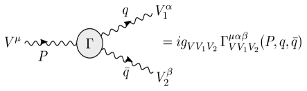
FIG. 1.: Feynman rule for the general $V\to V_{1}V_{2}$ vertex.

While the decomposition into form factors is general, convenient parameterizations of their low-energy behavior are provided by the effective Lagrangian approach [6]. Many different forms have been used in the literature. Here it suffices to use the phenomenological Lagrangian of Ref. [5] as an example. Keeping $C$ and $P$ conserving terms only, the $WWV$ vertex ($V=Z,\gamma$) is given in terms of three parameters, $g_{1}^{V}$, $\kappa_{V}$ and $\lambda_{V}$,

$${\cal L}_{eff}^{WWV} = i\,g_{WWV}\Bigl{(}\;g_{1}^{V}(W^{+}_{\mu\nu}W^{-\,\mu}-W^{+\,\mu}W^{-}_{\mu\nu})V^{\nu}+\kappa_{V}\,W^{+}_{\mu}W^{-}_{\nu}V^{\mu\nu}$$ (8)

$${\phantom{i\,g_{WWV}}}+{\lambda_{V}\over m_{W}^{2}}W_{\mu}^{+\,\nu}W_{\nu}^{-\,\rho}{V_{\rho}}^{\mu}\Bigr{)}\;,$$

where e.g. $V^{\mu\nu}=\partial^{\mu}V^{\nu}-\partial^{\nu}V^{\mu}$ is the $\gamma$ or $Z$ field strength tensor. Within the SM, the couplings are given by $g_{1}^{Z}=g_{1}^{\gamma}=\kappa_{Z}=\kappa_{\gamma}=1$, and $\lambda_{Z}=\lambda_{\gamma}=0$. The effective Lagrangian of Eq. 8 provides us with the lowest order terms in an expansion of the form factors $f_{i}$ in powers of the Lorentz invariants $P^{2}$, $q^{2}$ and $\bar{q}^{2}$. For (on- or off-shell) $W^{+}W^{-}$ production they are given by

$$f_{1}^{V}(P^{2},q^{2},\bar{q}^{2})\; \approx \;g_{1}^{V}+\,\lambda_{V}{P^{2}\over 2m_{W}^{2}}\;,$$ (9)

$$f_{2}^{V}(P^{2},q^{2},\bar{q}^{2})\; \approx \;\lambda_{V}\;,$$ (10)

$$f_{3}^{V}(P^{2},q^{2},\bar{q}^{2})\; \approx \;g_{1}^{V}+\,\kappa_{V}+\,\lambda_{V}{q^{2}+\bar{q}^{2}\over 2m_{W}^{2}}\;,$$ (11)

$$f_{4}^{V}(P^{2},q^{2},\bar{q}^{2})\; \approx \;-i\lambda_{V}{q^{2}-\bar{q}^{2}\over 2m_{W}^{2}}\;.$$ (12)

The notation developed up to here is getting cumbersome when comparing crossing related processes. The tensor decomposition of Eq. 6 treats incoming and outgoing vector bosons differently. As a result the form factors $f_{i}(P^{2},q^{2},\bar{q}^{2})$ are process dependent: they mix under crossing. It is more convenient to define form factors $g_{1}^{V}(P^{2},q^{2},\bar{q}^{2})$, $\kappa_{V}(P^{2},q^{2},\bar{q}^{2})$ and $\lambda_{V}(P^{2},q^{2},\bar{q}^{2})$ such that the relations of Eqs. 9–11 become exact for $V(P)\to W^{-}(q)W^{+}(\bar{q})$. This approach has the advantage that the Feynman rules derived from the effective Lagrangian of Eq. 8 can be used directly to calculate the full form factor dependence for any process involving $WWV$ vertices. At the same time the relations between form factors for crossing related processes become manifest. The only disadvantage is that the coupling constants appearing in the effective Lagrangian might be confused with the full form factors, while in reality they just represent the low energy limits of these form factors.

The functional behaviour of the form factors depends on the details of the underlying new physics. Effective Lagrangian techniques [6] are of little help here because the low energy expansion which leads to the effective Lagrangians exactly breaks down where the form factor effects become important. So in practice one will have to make ad hoc assumptions. One possibility is to assume a behaviour similar to nucleon form factors, with constraints derived from unitarity considerations [7]. Such constraints do become important at hadron colliders. More generally, they must be included when one searches for very large enhancements of vector boson pair production cross sections.

3. Vector Boson Pair Production

Deviations of the TGV’s from their SM, tree level form are most directly observed in vector boson pair production. Candidate processes are $W\gamma$, $WZ$ and $W^{+}W^{-}$ production at hadron colliders (namely the Tevatron and, eventually, the LHC) and $e^{+}e^{-}\to W^{+}W^{-}$ at LEP II or a NLC. Since experimental strategies have been discussed at great depth by other speakers at this symposium [8], I will concentrate here on some of the more basic effects of anomalous TGV’s on vector boson pair production.

3.1 $W^{+}W^{-}$ Production in $e^{+}e^{-}$ Collisions

To lowest order, the production of $W$ pairs in $e^{+}e^{-}$ collisions proceeds via the Feynman graphs of Fig. 2. It is instructive to consider the individual contributions of $s$-channel photon and $Z$ exchange and of $t$-channel neutrino exchange to the various helicity amplitudes [5],

FIG. 2.: Feynman graphs for the process $e^{+}e^{-}\to W^{+}W^{-}$.

$${\cal M}(\sigma,\lambda,\bar{\lambda})={\cal M}={\cal M}_{\gamma}+{\cal M}_{Z}+{\cal M}_{\nu}\;.$$ (13)

Here the $e^{-}$ and $e^{+}$ helicities are given by $\sigma/2$ and $-\sigma/2$, and $\lambda$ and $\bar{\lambda}$ denote the $W^{-}$ and $W^{+}$ helicities. Following Ref. [5] let us define reduced amplitudes $\tilde{\cal M}$ by splitting off the leading angular dependence in terms of the $d$-functions $d^{J_{0}}$ where $J_{0}=1,2$ denotes the lowest angular momentum contributing to a given helicity combination,

$${\cal M}(\sigma,\lambda,\bar{\lambda};\theta)=\sqrt{2}e^{2}\tilde{\cal M}_{\sigma,\lambda,\bar{\lambda}}(\theta)\;d^{J_{0}}_{\sigma,\lambda-\bar{\lambda}}(\theta)\;.$$ (14)

$s$-channel photon and $Z$ exchange is only possible for $|\lambda-\bar{\lambda}|=0,1$. The corresponding reduced amplitudes can be written as

$$\tilde{\cal M}_{\gamma} = -\beta A^{\gamma}_{\lambda\bar{\lambda}}\;,$$ (15)

$$\tilde{\cal M}_{Z} = +\beta A^{Z}_{\lambda\bar{\lambda}}\left[1-\delta_{\sigma,-1}{1\over 2\,{\rm sin}^{2}\theta_{W}}\right]{s\over s-m_{Z}^{2}}\;,$$ (16)

$$\tilde{\cal M}_{\nu} = +\delta_{\sigma,-1}{1\over 2\beta\,{\rm sin}^{2}\theta_{W}}\left[B_{\lambda\bar{\lambda}}-{1\over 1+\beta^{2}-2\beta{\rm cos}\theta}C_{\lambda\bar{\lambda}}\right]\;.$$ (17)

Here $s$ denotes the $e^{+}e^{-}$ center of mass energy and $\beta=\sqrt{1-4m_{W}^{2}/s}$ is the $W^{\pm}$ velocity. The subamplitudes $A^{V}$, $B$ and $C$ are given in Table I.

TABLE I.: Subamplitudes for $J_{0}=1$ helicity combinations of the process $e^{-}e^{+}\to W^{-}W^{+}$, as defined in Eq. 17. $\beta$ denotes the $W$ velocity and $\gamma=\sqrt{s}/2m_{W}$. The relations between the form factors $f_{i}$ and $g_{1}$, $\kappa$, and $\lambda$ are given in Eqs. 9–11, with $q^{2}=\bar{q}^{2}=m_{W}^{2}$.

$\lambda\bar{\lambda}$	$A^{V}_{\lambda\bar{\lambda}}$	$B_{\lambda\bar{\lambda}}$	$C_{\lambda\bar{\lambda}}$
$++$	$g_{1}^{V}+2\gamma^{2}\lambda_{V}+{i\over\beta}f_{6}^{V}+4i\gamma^{2}\beta f_{7}^{V}$	$1$	$1/\gamma^{2}$
$--$	$g_{1}^{V}+2\gamma^{2}\lambda_{V}-{i\over\beta}f_{6}^{V}-4i\gamma^{2}\beta f_{7}^{V}$	$1$	${1/\gamma^{2}}$
$+0$	$\gamma(f_{3}^{V}-if_{4}^{V}+\beta f_{5}^{V}+{i\over\beta}f_{6}^{V})$	$2\gamma$	$2(1+\beta)/\gamma$
$0-$	$\gamma(f_{3}^{V}+if_{4}^{V}+\beta f_{5}^{V}-{i\over\beta}f_{6}^{V})$	$2\gamma$	$2(1+\beta)/\gamma$
$0+$	$\gamma(f_{3}^{V}+if_{4}^{V}-\beta f_{5}^{V}+{i\over\beta}f_{6}^{V})$	$2\gamma$	$2(1-\beta)/\gamma$
$-0$	$\gamma(f_{3}^{V}-if_{4}^{V}-\beta f_{5}^{V}-{i\over\beta}f_{6}^{V})$	$2\gamma$	$2(1-\beta)/\gamma$
$00$	$g_{1}^{V}+2\gamma^{2}\kappa_{V}$	$2\gamma^{2}$	${2/\gamma^{2}}$

One of the most striking features of the SM are the gauge theory cancellations between $\gamma$, $Z$ and neutrino exchange graphs. Within the SM $g_{1}=\kappa=1,\;\lambda=0$ (or $f_{1}=1$, $f_{2}=0$, $f_{3}=2$) for both the photon and the $Z$-exchange graphs. As a result $A^{\gamma}_{\lambda\bar{\lambda}}=A^{Z}_{\lambda\bar{\lambda}}$ and the $\beta A^{V}$ terms in Eq. 17 cancel, except for the difference between photon and $Z$ propagators. Similarly, the $B_{\lambda\bar{\lambda}}$ term in $\tilde{\cal M}_{\nu}$ and the $\delta_{\sigma,-1}$ term in $\tilde{\cal M}_{Z}$ cancel in the high energy limit for all helicity combinations. While the contributions from individual Feynman graphs grow with energy for longitudinally polarized $W$’s, this unacceptable high energy behavior is avoided in the full amplitude due to the cancellations which can be traced to the gauge theory relations between fermion–gauge boson vertices and the TGV’s.

At asymptotically large energies any deviations of $f_{3}$, … $f_{6}$ from their SM values would lead to a growth of at least some of the helicity amplitudes $\tilde{\cal M}_{0\pm}$ or $\tilde{\cal M}_{\pm 0}$ with energy and hence violate partial wave unitarity. Similarly, non-standard values of $f_{7}$, $\lambda$ or $\kappa$ in the $s\to\infty$ limit would lead to an unacceptable growth in some of the remaining three helicity amplitudes. Thus, in this limit, partial wave unitarity excludes anomalous TGV’s [9]; any deviation from the SM must be described by an energy-dependent form factor which approaches its gauge theory value as $s\to\infty$.

Table I shows that only seven $W^{-}W^{+}$ helicity combinations contribute to the $J=1$ channel and the form factors $f_{i}$ enter in as many different combinations. This explains why exactly seven form factors or coupling constants are needed to parameterize the most general $WWV$ vertex. Since we have both $WWZ$ and $WW\gamma$ couplings at our disposal, the most general $J=1$ amplitudes ${\cal M}_{L}={\cal M}(\sigma=-1,\lambda,\bar{\lambda})$ and ${\cal M}_{R}={\cal M}(\sigma=+1,\lambda,\bar{\lambda})$ for both left- and right-handed incoming electrons can be parameterized. Turning the argument around one concludes that all 14 helicity amplitudes need to be measured independently for a complete determination of all the form factors $f_{i}^{\gamma}(s)$ and $f_{i}^{Z}(s)$, at any value of the center of mass energy, $\sqrt{s}$.

Formidable as this goal may be it can be approached to a remarkable degree by performing a partial wave analysis, in particular of the semileptonic process $e^{-}e^{+}\to W^{-}W^{+}\to\ell^{\pm}\nu q\bar{q}^{\prime}$. The charge of the lepton allows to identify the two $W$ charges and hence the production angle $\theta$. From Eq. 14 one finds that the $J=1$ amplitudes lead to the angular distribution

$${d\sigma\over d{\rm cos}\theta} \sim {{\rm sin}^{2}\theta\over 2}\left(|\tilde{\cal M}_{\sigma,++}|^{2}+|\tilde{\cal M}_{\sigma,--}|^{2}+|\tilde{\cal M}_{\sigma,00}|^{2}\right)$$ (20)

$$+{(1+\sigma\,{\rm cos}\,\theta)^{2}\over 4}\left(|\tilde{\cal M}_{\sigma,+0}|^{2}+|\tilde{\cal M}_{\sigma,0-}|^{2}\right)$$

$$+{(1-\sigma\,{\rm cos}\,\theta)^{2}\over 4}\left(|\tilde{\cal M}_{\sigma,0+}|^{2}+|\tilde{\cal M}_{\sigma,-0}|^{2}\right)\;.$$

Hence the amplitudes with different values of $|\lambda-\bar{\lambda}|$ can be separated, even though in practice one must take into account the additional $\theta$-dependence of the known neutrino exchange graphs, as is evident from Fig. 3.

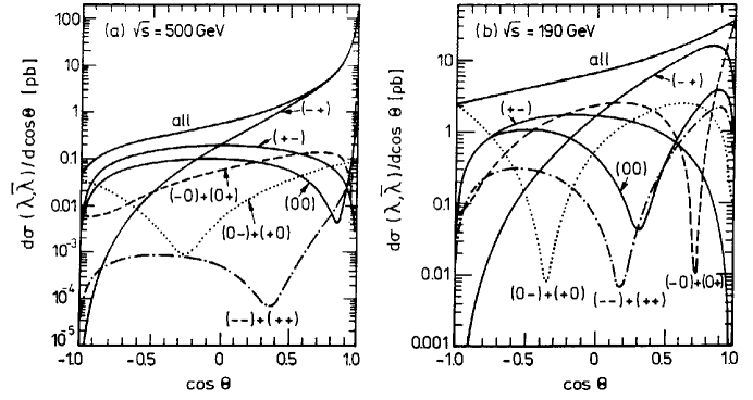
FIG. 3.: Angular distributions $d\sigma/d{\rm cos}\theta$ for fixed $W^{-}W^{+}$ helicities $(\lambda\bar{\lambda})$ in $e^{-}e^{+}$ collisions at a) $\sqrt{s}=500$ GeV and b) $\sqrt{s}=190$ GeV. From Ref. [5].

Due to the $V-A$ structure of the $W$–fermion vertices the decay angular distributions of the $W$’s are excellent polarization analyzers. Consider for example the polar angle $\theta_{-}$ of the charged lepton $\ell^{-}$ in the $W^{-}$ rest frame with respect to the $W^{-}$ direction in the lab frame. Its distribution is proportional to $(1-\lambda{\rm cos}\theta_{-})^{2}$ for transversely polarized $W^{-}$ and proportional to ${\rm sin}^{2}\theta_{-}$ for longitudinally polarized $W^{-}$. Combined with the information contained in the production angle distribution, the individual helicity amplitudes can be isolated, at least when polarized electron beams are available.

In practice, statistical errors will limit the accuracy with which such an analysis can be carried out. The best sensitivity to anomalous contributions is achieved when interference with large SM amplitudes can be exploited. Unfortunately, the dominant SM amplitudes are the $J_{0}=2$ amplitudes ${\cal M}_{+-}$ and ${\cal M}_{-+}$ which are purely due to $t$-channel neutrino exchange (see Fig. 3). At asymptotically large energies the only surviving $J=1$ helicity amplitude is ${\cal M}_{00}$ and even its contribution is small numerically. Polar angle distributions alone yield relatively low sensitivity to anomalous TGV’s.

The way out is to measure azimuthal angle distributions and azimuthal angle correlations which exploit the interference of the various $J=1$ amplitudes with the $t$-channel neutrino exchange graph. In order to independently measure the various form-factors it is necessary to measure the full five-fold angular distributions

$${d^{5}\sigma\over d{\rm cos}\theta\;d{\rm cos}\theta_{+}\;d\phi_{+}\;d{\rm cos}\theta_{-}\;d\phi_{-}}\;,$$ (21)

or more precisely the projection of this five-fold angular distribution on the triple $J=1$ partial wave.

The sensitivity of such an analysis has been investigated for both LEP II and NLC energies [10, 11]. One finds, for example, that $\Delta\kappa$ should be measurable with an accuracy of $\approx 5\cdot 10^{-4}$ at a $1.5$ TeV NLC [11]. Does this mean that electroweak radiative corrections will be probed by measuring $W^{+}W^{-}$ production at a NLC? In spite of the small value of $\Delta\kappa$ this is not necessarily the case. According to Table I, an anomalous value of $\Delta\kappa$ has its largest effect on $W_{L}W_{L}$ production. With $\gamma=\sqrt{s}/2m_{W}\approx 10$ and taking the gauge theory cancellations into account, the effect of $\Delta\kappa=5\cdot 10^{-4}$ on ${\cal M}_{00}$ is proportional to

$$\tilde{\cal M}_{00}\sim{m_{Z}^{2}\over 2m_{W}^{2}}+2\gamma^{2}\Delta\kappa=0.65+2\cdot 10^{2}\cdot 5\cdot 10^{-4}=0.65\cdot 1.15\;,$$ (22)

$i.e.$ the anomalous TGV corresponds to a change of the $W_{L}W_{L}$ amplitude of 15%, which probably is more than should be expected from electroweak radiative corrections.

3.2 Weak Boson Pair Production at Hadron Colliders

There are substantial differences in the study of TGV’s at $e^{+}e^{-}$ vs. hadron colliders. At LEP II or a NLC a detailed study of individual helicity amplitudes is possible and hence the individual form factors can be separated at any center of mass energy $\sqrt{s}$. In the clean environment of these machines errors are largely dominated by statistics and weak boson pair production cross sections can hence be measured with errors in the few percent range, i.e. the search for anomalous TGV’s corresponds to the search of ${\cal O}(10^{-2})$ deviations of the production cross sections from the SM predictions.

Hadron colliders like the Tevatron or the LHC allow to study all pair production processes: $W^{+}W^{-}$, $W^{\pm}\gamma$, and $W^{\pm}Z$ production. Via the last two processes one can thus independently measure $WW\gamma$ and $WWZ$ vertices. At the same time larger center of mass energies are available at the hadron machines compared to their $e^{+}e^{-}$ contemporaries and hence the form factors are explored at higher energy scales. In turn this implies large enhancement factors ($\gamma$ or $\gamma^{2}$) for the anomalous contributions. The signals we are searching for appear in the $J=1$ partial wave $i.e.$ for large production angles of the final state electroweak bosons and they are enhanced at large c.m. energies. Both features move observable effects to large transverse momenta of the produced vector bosons or their decay products. This effect is demonstrated in Fig. 4 where expected transverse momentum distributions in $p\bar{p}\to W^{+}\gamma$ and $p\bar{p}\to W^{+}Z$ production at the Tevatron are shown for several choices of anomalous couplings and dipole form factors $\Delta f_{i}(s)=\Delta f_{i}^{0}/(1+s/1{\rm TeV}^{2})^{2}$.

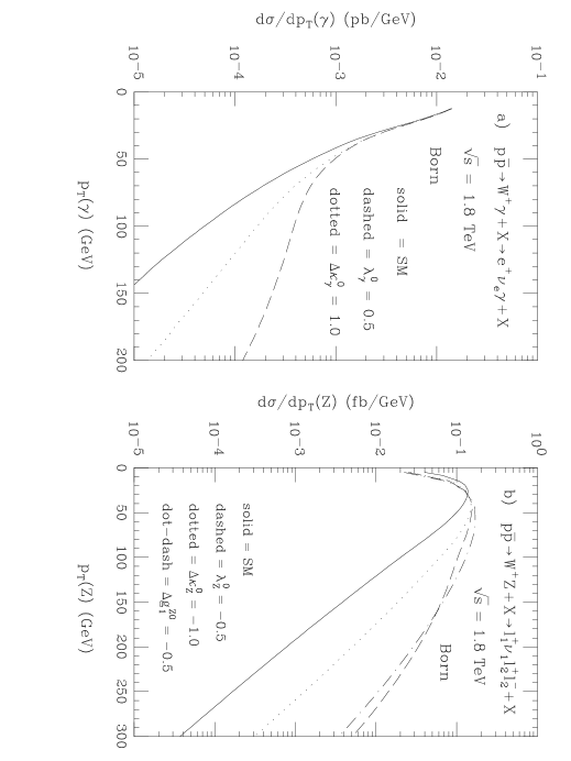
FIG. 4.: Transverse momentum distribution of a) the photon in $W^{+}\gamma$ production and b) the $Z$ in $W^{+}Z$ production in $p\bar{p}$ collisions at the Tevatron for various sets of anomalous coupling parameters. From Ref. [2].

Due to the more difficult background situation and also because of insufficient knowledge of QCD radiative corrections [12], structure function effects etc., a comparison of measured and theoretically predicted cross sections at the ${\cal O}(10^{-2})$ level is not feasible at hadron colliders. Rather their sensitivity to anomalous TGV’s derives from fairly large deviations from the SM in at least some regions of phase space. A typical example is shown in Fig. 4 where for most choices of anomalous couplings $d\sigma/dp_{T}(V)$ is increased by one order of magnitude or more in parts of the accessible transverse momentum range.

The actual shape of the $p_{T}$ distributions depends crucially on the energy dependence of the form factors. In weakly interacting models of new physics (like supersymmetry [13]) one should expect that virtual effects of heavy particles (of mass $M$) will never lead to changes of cross sections by such large factors. At low energy anomalous couplings are expected to scale like [14]

$$\Delta f_{i}(0)\sim{g^{2}\over 16\pi^{2}}{m_{W}^{2}\over M^{2}}\;,$$ (23)

while, at energies above the heavy particle mass $M$, form factor damping will set in and qualitatively a behaviour like

$$\Delta f_{i}(s>>M^{2})\sim{g^{2}\over 16\pi^{2}}{m_{W}^{2}\over s}$$ (24)

must be expected. Turning to the effect on the weak boson pair production cross section one finds that even when including a $\gamma^{2}=s/4m_{W}^{2}$ enhancement factor in the amplitude, the amplitude changes only by a term of order

$$\Delta{\cal M}\sim{s\over m_{W}^{2}}\Delta f_{i}(s) \sim {g^{2}\over 16\pi^{2}}{s\over M^{2}}\quad{\rm for}\;\;s<<M^{2}\;,$$ (26)

$${g^{2}\over 16\pi^{2}}{\phantom{s\over M^{2}}}\quad{\rm for}\;\;s>>M^{2}\;,$$

and the change in the amplitude is at most of the order of the naive perturbative expectation, $g^{2}/16\pi^{2}$. Thus, for weakly coupled new physics, no large enhancement of weak boson pair production cross sections occurs. The dramatic increase of $WZ$ or $W\gamma$ production rates shown in Fig. 4 needs some strong interaction dynamics in the weak boson sector, and even then it is not guaranteed to occur [14].

One thus finds that in their search for anomalous TGV’s $e^{+}e^{-}$ and hadron colliders are complementary. LEP or a 500 GeV NLC will probe $W^{+}W^{-}$ pair production cross sections quite precisely, but at relatively low center of mass energies. This limits the enhancement factors for anomalous TGV’s but, with sufficient statistics, even relatively weakly coupled new physics may be accessible. At the hadron colliders much higher energy ranges can be probed, but these experiments are only sensitive to strongly coupled new physics.

4. Finite Width Effects and Gauge Invariance

Some of the features of anomalous couplings, namely form factors and the necessity to consider the full $S$-matrix elements can nicely be illustrated by some very non-anomalous physics, namely fermion loop corrections within the SM. At the same time I would like to address the problem of how to implement finite width effects while maintaining gauge invariance when dealing with processes involving TGV’s [15]. The discussion will closely follow Ref. [16].

Let us consider $W\gamma$ production at hadron colliders as an example. Denoting the photon polarization vector by $\varepsilon^{*\mu}$ we can write the amplitude as

$${\cal M}=\varepsilon_{\mu}^{*}{\cal M}^{\mu}=\varepsilon_{\mu}^{*}{\cal M}_{q}^{\mu}+\varepsilon_{\mu}^{*}{1\over\hat{s}-m_{W}^{2}}{\cal M}_{W}^{\mu}\;,$$ (27)

where ${\cal M}_{q}$ denotes $t$- and $u$-channel quark exchange graphs and ${\cal M}_{W}$ stands for the $s$-channel $W$ exchange graph which involves the TGV. Electromagnetic gauge invariance is guaranteed by the relation

$$k_{\mu}{\cal M}^{\mu}=k_{\mu}{\cal M}_{q}^{\mu}+k_{\mu}{1\over\hat{s}-m_{W}^{2}}{\cal M}_{W}^{\mu}=0\;.$$ (28)

Replacing the $W$ propagator factor by a Breit-Wigner form, $1/(\hat{s}-m_{W}^{2}+im_{W}\Gamma_{W})$, disturbs the gauge cancellations between the individual Feynman graphs and thus leads to an amplitude which is not electromagnetically gauge invariant. In addition, a constant imaginary part in the inverse propagator is ad hoc: it results from fermion loop contributions to the $W$ vacuum polarization and the imaginary part should vanish for space-like momentum transfers.

The general structure is best understood by first considering the lower order process $q\bar{q}^{\prime}\to W^{-}\to\ell^{-}\bar{\nu}$ without photon emission (see Fig. 5). Finite width effects are included by resumming the imaginary parts of the fermion loops. Neglecting fermion masses, the transverse part of the $W$ vacuum polarization receives an imaginary contribution

$$Im\,\Pi_{W}^{T}(q^{2})=\sum_{f}{g^{2}\over 48\pi}q^{2}=q^{2}{\Gamma_{W}\over m_{W}}\;,$$ (29)

while the imaginary part of the longitudinal piece vanishes. In the unitary gauge and for $q^{2}>0$ the $W$ propagator is thus given by

$$D_{W}^{\mu\nu}(q) = {-i\over q^{2}-m_{W}^{2}+iIm\,\Pi_{W}^{T}(q^{2})}\left(g^{\mu\nu}-{q^{\mu}q^{\nu}\over q^{2}}\right)+{i\over m_{W}^{2}-iIm\,\Pi_{W}^{L}(q^{2})}\;{q^{\mu}q^{\nu}\over q^{2}}$$ (30)

$$= {-i\over q^{2}-m_{W}^{2}+iq^{2}\gamma_{W}}\left(g^{\mu\nu}-{q^{\mu}q^{\nu}\over m_{W}^{2}}(1+i\gamma_{W})\right)\;,$$ (31)

where the abbreviation $\gamma_{W}=\Gamma_{W}/m_{W}$ has been used. Note that the $W$ propagator has received a $q^{2}$ dependent effective width which actually would vanish in the space-like region.

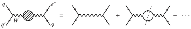
FIG. 5.: Feynman graphs for the process $q\bar{q}^{\prime}\to\ell^{-}\bar{\nu}$ at lowest order. The resummation of the imaginary part of the $W$ vacuum polarization leads to the Breit-Wigner type $W$ propagator of Eq. 31 which is represented by the shaded blob.

Now consider the same process, but including photon emission. A gauge invariant expression is obtained by attaching the final state photon in all possible ways to all charged particle propagators in the Feynman graphs of Fig. 5. This includes radiation off the two incoming quark lines, radiation off the final state charged lepton, and radiation off the $W$ propagators. In addition, the photon must be attached to the charged fermions inside the $W$ vacuum polarization loops, leading to the fermion triangle graphs of Fig. 6. For a consistent treatment we only need to include the imaginary part of the triangle graphs which is obtained by cutting the triangle graphs into on-shell intermediate states in all possible ways, as shown in the figure.

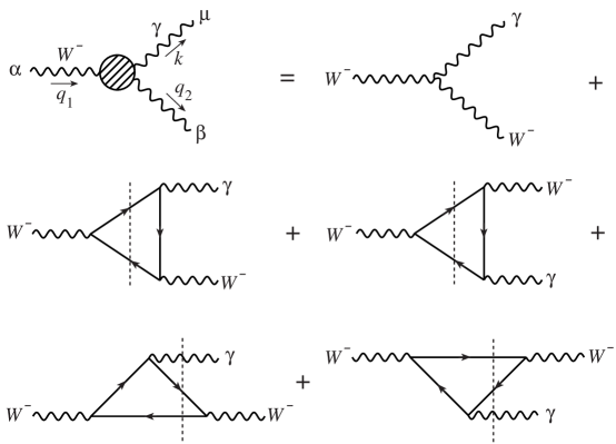
FIG. 6.: Effective $WW\gamma$ vertex as needed in the tree level calculation of $W\gamma$ production. In addition to the lowest order vertex the imaginary parts of the fermion triangles must be included (see Eq. 33).

For the momentum flow of Fig. 6 the lowest order vertex is given by the familiar expression

$$-ie\Gamma_{0}^{\alpha\beta\mu}=-ie\left((q_{1}+q_{2})^{\mu}g^{\alpha\beta}-(q_{1}+k)^{\beta}g^{\mu\alpha}+(k-q_{2})^{\alpha}g^{\mu\beta}\right)\;.$$ (32)

Neglecting the masses of the fermions in the triangle graphs and dropping terms proportional to $k^{\mu}$ (which will be contracted with the photon polarization vector $\varepsilon^{*\mu}$ and hence vanish in the amplitude) the contributions from the four triangle graphs reduce to an extremely simple form. Each fermion doublet $f$, irrespective of its hypercharge, adds $i(g^{2}/48\pi)\Gamma_{0}$ to the lowest order $WW\gamma$ vertex $\Gamma_{0}$. After summing over all fermion species, the lowest order vertex is thus replaced by

$$\Gamma^{\alpha\beta\mu}=\Gamma_{0}^{\alpha\beta\mu}\left(1+\sum_{f}{ig^{2}\over 48\pi}\right)=\Gamma_{0}^{\alpha\beta\mu}\left(1+i\,{\Gamma_{W}\over m_{W}}\right)=\Gamma_{0}^{\alpha\beta\mu}\left(1+i\gamma_{W}\right)\;.$$ (33)

By construction, the resulting amplitude for the process $q\bar{q}^{\prime}\to\ell^{-}\bar{\nu}\gamma$ is gauge invariant. Indeed, gauge invariance of the full amplitude can be traced to the electromagnetic Ward identity [17]

$$k_{\mu}{\Gamma_{\alpha\beta}}^{\mu}=\left(iD_{W}\right)^{-1}_{\alpha\beta}(q_{1})-\left(iD_{W}\right)^{-1}_{\alpha\beta}(q_{2})\;.$$ (34)

Since

$$k_{\mu}\Gamma^{\alpha\beta\mu}=\left((q_{1}^{2}g^{\alpha\beta}-q_{1}^{\alpha}q_{1}^{\beta})-(q_{2}^{2}g^{\alpha\beta}-q_{2}^{\alpha}q_{2}^{\beta})\right)\left(1+i\gamma_{W}\right)\;,$$ (35)

and

$$\left(iD_{W}\right)^{-1}_{\alpha\beta}(q)=\left(q^{2}-m_{W}^{2}+iq^{2}\gamma_{W}\right)\left(g_{\alpha\beta}-{q_{\alpha}q_{\beta}\over q^{2}}\right)-m_{W}^{2}{q_{\alpha}q_{\beta}\over q^{2}}\;,$$ (36)

this Ward identity is satisfied by our $W$ propagator and $WW\gamma$ vertex.

The modification of the lowest order $WW\gamma$ vertex in Eq. 33 looks like the introduction of anomalous couplings $g_{1}^{\gamma}=\kappa_{\gamma}=1+i\gamma_{W}$ and one may thus worry that the full amplitude will violate unitarity at large center of mass energies $\sqrt{\hat{s}}$. While indeed the vertex is modified, this modification is compensated by the effective $\hat{s}$-dependent width in the propagator. As compared to the expressions with a lowest order propagator, $1/(\hat{s}-m_{W}^{2})$, which of course has good high energy behaviour, the overall effect is multiplication of the $s$-channel $W$-exchange amplitude ${\cal M}_{W}$ by a factor

$$G(\hat{s})={\hat{s}-m_{W}^{2}\over\hat{s}(1+i\gamma_{W})-m_{W}^{2}}\;(1+i\gamma_{W})=1\;-\;{i\Gamma_{W}m_{W}\over\hat{s}-m_{W}^{2}+im_{W}\Gamma_{W}{\hat{s}\over m_{W}^{2}}}\;.$$ (37)

Obviously, $G(\hat{s})\to 1$ as $\hat{s}\to\infty$ and the high energy behaviour of our finite width amplitude is identical to the one of the naive tree level result for $W\gamma$ production. In fact, the contributions from the triangle graphs are crucial to compensate the bad high energy behaviour introduced by the $q^{2}$-dependent width in Eq. 31.

This interplay of propagator and vertex corrections illustrates the remarks made in Section 2. The leading one-loop contributions, namely the imaginary parts of $WW\gamma$ vertex and inverse $W$ propagator, lead to a change of the $S$-matrix element for $W\gamma$ production which can be parameterized in terms of the generalized vertex function $\Gamma^{\mu\alpha\beta}_{\gamma WW}(k,q_{1},q_{2})$. The nonvanishing form factors in its tensor decomposition are given by

$$g_{1}^{\gamma}(q_{1}^{2})=\kappa_{\gamma}(q_{1}^{2})=G(q_{1}^{2})=1\;-\;{i\Gamma_{W}m_{W}\over q_{1}^{2}-m_{W}^{2}+i{\Gamma_{W}\over m_{W}}q_{1}^{2}}\;,$$ (38)

and the form factor scale is set by the masses of the particles involved, here the $W$ boson mass.

5. Conclusions

The direct measurement of the nonabelian $WW\gamma$ and $WWZ$ vertices at present and future hadron and $e^{+}e^{-}$ colliders constitutes an important test of the basic structure of electroweak interactions. There are strong theoretical arguments that experiments will yield exactly the results predicted by the SM, even though no rigorous proof of this assertion exists. Observation of anomalous couplings at either the Tevatron or at LEP II would therefore have grave consequences for our understanding of electroweak physics.

Irrespective of how likely an observation of anomalous couplings might be, $e^{+}e-$ and hadron colliders measure very different aspects of $WWV$ vertex functions. With sufficient statistics $e^{+}e^{-}$ experiments are able to probe small deviations from SM cross sections and are hence sensitive to weakly interacting new physics. However, they will mainly probe just one process, $W$ pair production, in a limited energy range. Hadron colliders, on the other hand, can investigate all electroweak boson pair production processes, albeit with lower accuracy. They look for relatively large enhancements of cross sections at high center of mass energies and are thus only sensitive to new strong interaction dynamics in the bosonic sector. Hadron and $e^{+}e^{-}$ machines are indeed complementary means to directly study the nonabelian aspects of electroweak interactions.

REFERENCES

- [1] D. Schaile, these proceedings.
- [2] H. Aihara et al., report of the DPF study subgroup on Anomalous Gauge Boson Interactions, report MAD/PH/871 (1995) (hep-ph/9503425) and references therein.
- [3] P. Hernandez, these proceedings.
- [4] K. Gaemers and G. Gounaris, Z. Phys. C1, 259 (1979).
- [5] K. Hagiwara, K. Hikasa, R.D. Peccei, and D. Zeppenfeld, Nucl. Phys. B282, 253 (1987).
- [6] J. Wudka, these proceedings.
- [7] M. Suzuki, Phys. Lett. B153, 289 (1985); C. Bilchak, M. Kuroda and D. Schildknecht, Nucl. Phys. B299, 7 (1988); U. Baur and D. Zeppenfeld, Phys. Lett. 201B, 383 (1988); U. Baur and E. Berger, Phys. Rev. D47, 4889 (1993).
- [8] See the contributions by H. Aihara, T. Barklow, J. Busenitz, T. Fuess, S. Godfrey, T. Han, H. Johari, G. Landsberg, D. Neuberger, A. Schöning, G. Valencia, R. Wagner, R. Walczak, C. Wendt, J. Womersley, and L. Zhang in these proceedings.
- [9] J. M. Cornwall, D. N. Levin, and G. Tiktopoulos, Phys. Rev. Lett. 30, 1268 (1973), Phys. Rev. D10, 1145 (1974); C. H. Llewellyn Smith, Phys. Lett. 46B, 233 (1973); S. D. Joglekar, Ann. Phys. 83 (1974) 427.
- [10] See e.g. M. Bilenkii, J. L. Kneur, F. M. Renard and D. Schildknecht, Nucl. Phys. B409, 22 (1993), ibid. B419, 240 (1994); R. L. Sekulin, Phys. Lett. B338, 369 (1994); M. Diehl and O. Nachtmann, Z. Phys. C62, 397 (1994); J. Busenitz; S. Godfrey, these proceedings.
- [11] T. Barklow, these proceedings.
- [12] J. Ohnemus, these proceedings.
- [13] A. Lahanas, these proceedings.
- [14] C. Arzt, M. B. Einhorn, and J. Wudka, Phys. Rev. D49, 1370 (1994); Nucl. Phys. B433, 41 (1995); M. B. Einhorn and J. Wudka, preprints NSF-ITP-92-01 (1992) and UM-TH-92-25 (1992); J. Wudka, Int. J. Mod. Phys. A9, 2301 (1994).
- [15] See e.g. A. Aeppli, F. Cuypers and G. J. van Oldenborgh, Phys. Lett. B314, 413 (1993).
- [16] U. Baur and D. Zeppenfeld, report MAD/PH/878 (1995), (hep-ph/9503344).
- [17] See e.g. G. Lopez Castro, J.L.M. Lucio, and J. Pestieau, Mod. Phys. Lett. A6, 3679 (1991); M. Nowakowski and A. Pilaftsis, Z. Phys. C60, 121 (1993) and references therein.