Abstract

We present a systematic phenomenological analysis of the tests of CPT symmetry that are possible within an open quantum-mechanical description of the neutral kaon system that is motivated by arguments based on quantum gravity and string theory. We develop a perturbative expansion in terms of the three small CPT-violating parameters admitted in this description, and provide expressions for a complete set of $K\rightarrow 2\pi,3\pi$ and $\pi\ell\nu$ decay observables to second order in these small parameters. We also illustrate the new tests of CPT symmetry and quantum mechanics that are possible in this formalism using a regenerator. Indications are that experimental data from the CPLEAR and previous experiments could be used to establish upper bounds on the CPT-violating parameters that are of order $10^{-19}$ GeV, approaching the order of magnitude that may be attainable in quantum theories of gravity.

1 Introduction

The neutral kaon system has long served as a penetrating probe of fundamental physics. It has revealed or illuminated many new areas of fundamental physics, including parity violation, CP violation, flavour-changing neutral interactions, and charm. It remains the most sensitive test of fundamental symmetries, being the only place where CP violation has been observed, namely at the level of $10^{-18}$ GeV in the imaginary part of the effective mass matrix for neutral kaons, and providing the most stringent microscopic check of CPT symmetry within the framework of quantum mechanics, namely $|(m_{K^{0}}-m_{\bar{K}^{0}})/m_{K^{0}}|<9\times 10^{-19}$ [1].

It is well known that CPT symmetry is a fundamental theorem of quantum field theory, which follows from locality, unitarity, and Lorentz invariance [2]. However, the topic of CPT violation has recently attracted increased attention, drawn in part by the prospect of higher-precision tests by CPLEAR [3] and at DA$\Phi$NE [4], and in part by the renewed theoretical interest in quantum gravity motivated by recent developments in string theory. Some of the phenomenological discussion has been in the context of quantum mechanics [5], abandoning implicitly or explicitly the derivation of quantum mechanics from quantum field theory, in which CPT is sacrosanct. Instead, we have followed the approach of Ref. [6], in which a parametrization of CPT-violating effects is introduced via a deviation from conventional quantum mechanics [6, 7] believed to reflect the loss of quantum coherence expected in some approaches to quantum gravity [8], notably one based on a non-critical formulation of string theory [9].

The suggestion that quantum coherence might be lost at the microscopic level was made in Ref. [8], which suggested that asymptotic scattering should be described in terms of a superscattering operator $S\hskip-8.0pt/\hskip 2.0pt$, relating initial $(\rho_{\rm in})$ and final $(\rho_{\rm out})$ density matrices, that does not factorize as a product of $S$- and $S^{\dagger}$-matrix elements:

$$\rho_{\rm out}=S\hskip-8.0pt/\hskip 2.0pt\rho_{\rm in}:\quad S\hskip-8.0pt/\hskip 2.0pt\not=SS^{\dagger}\ .$$ (1)

The loss of quantum coherence was thought to be a consequence of microscopic quantum-gravitational fluctuations in the space-time background. Model calculations supporting this suggestion were presented [8] and contested [10]. Ref. [6] pointed out that if Eq. (1) is correct for asymptotic scattering, there should be a corresponding effect in the quantum Liouville equation that describes the time-evolution of the dentity matrix $\rho(t)$:

$${\partial\rho(t)\over\partial t}=i[\rho,H]+i{\delta H\hskip-8.5pt/\hskip 2.0pt}\rho\ ,$$ (2)

which is characteristic of an open quantum-mechanical system. Ref. [6] parametrized the non-Hamiltonian term in the case of a simple two-state system such as the $K^{0}-\bar{K}^{0}$ system, presented a first analysis of its phenomenological consequences, and gave experimental bounds on the non-quantum-mechanical parameters.

The question of microscopic quantum coherence has recently been addressed in the context of string theory using a variety of approaches [11]. In particular, we have analyzed this question using non-critical string theory [12], with criticality restored by non-trivial dynamics for a time-like Liouville field [12, 13], which we identify with the world-sheet cutoff and the target time variable [7, 9]. This approach leads to an equation of the form (2), in which probability and energy are conserved, and the possible magnitude of the extra term $|\delta H\hskip-8.5pt/\hskip 2.0pt|={\cal O}(E^{2}/M_{Pl})$, where $E$ is a typical energy scale of the system under discussion. The details of this approach are not essential for the phenomenological discussion of this paper, but it is interesting to note that the experimental sensitivity may approach this theoretical magnitude.

It has been pointed out [14] that at least the strong version of the CPT theorem must be violated in any theory described by a non-factorizing superscattering matrix $S\hskip-8.0pt/\hskip 2.0pt$ (1), which leads to a loss of quantum coherence. This is also true of the parametrization proposed by Ref. [6], which violates CPT in an intrinsically non-quantum-mechanical way. More detailed descriptions of phenomenological implications and improved experimental bounds were presented in Ref. [15]. These results were based on an analysis of $K_{L}$ and $K_{S}$ decays, and did not consider the additional constraints obtainable from an analysis of intermediate-time data. A systematic approach to the time evolution of the density matrix for the neutral kaon system was proposed in Ref. [16], and preliminary estimates of the improved experimental constraints on the non-quantum-mechanical parameters were presented. Similar results were presented later in Ref. [17], which also discussed correlation measurements possible at a $\phi$ factory such as DA$\Phi$NE.

The main focus of this paper is to present detailed formulae for the time dependences of several decay asymmetries that can be measured by the CPLEAR and DA$\Phi$NE experiments, using the systematic approach proposed in Ref. [16] and described in Section 3. In particular, we discuss in Section 4 the asymmetries known as $A_{2\pi},A_{3\pi},A_{\rm T},A_{\rm CPT}$ and $A_{\Delta m}$, whose definitions are reviewed in Section 2. We show in Section 5 that experiments with a regenerator can provide useful new measurements of the non-quantum-mechanical CPT-violating parameters. Then, in Section 6 we derive illustrative bounds on the non-quantum-mechanical parameters from all presently available data. Section 7 contains a brief discussion of the extension of the formalism of Ref. [6] to the correlation measurements possible at $\phi$ factories such as DA$\Phi$NE. We emphasize the need to consider a general parametrization of the two-particle density matrix, that cannot be expressed simply in terms of the previously-introduced single-particle density matrix parameters, and enables energy conservation to be maintained, as we have demonstrated [7, 9] in our non-critical string theory approach to the loss of quantum coherence. In Section 8 we review our conclusions and discuss the prospects for future experimental and theoretical work. Formulae for the CPLEAR observables in the context of standard quantum-mechanical CPT violation [5] are collected in Appendix A, where bounds on the corresponding parameters are also obtained. Lastly, complete formulae for the second-order contributions to the density matrix in our quantum-mechanical-violating framework are collected in Appendix B.

2 Formalism and Relevant Observables

In this section we first review aspects of the modifications (2) of quantum mechanics believed to be induced by quantum gravity [6], as argued specifically in the context of a non-critical string analysis [7, 9]. This provides a specific form for the modification (2) of the quantum Liouville equation for the temporal evolution of the density matrix of observable matter [7, 9]

$$\frac{\partial}{\partial t}\rho=i[\rho,H]+i{\delta H\hskip-8.5pt/\hskip 2.0pt}\rho\qquad;\qquad\delta H\hskip-8.5pt/\hskip 2.0pt\equiv{\dot{g}}^{i}G_{ij}[g^{i},\rho]$$ (3)

where the coordinates $\{g^{i}\}$ parametrize the space of possible string models and the extra term $\delta H\hskip-8.5pt/\hskip 2.0pt$ is such that the time evolution has the following basic properties:

(i) The total probability is conserved in time

$$\frac{\partial}{\partial t}{\rm Tr}\,\rho=0$$ (4)

(ii) The energy $E$ is conserved on the average

$$\frac{\partial}{\partial t}{\rm Tr}\,(E\rho)=0$$ (5)

as a result of the renormalizability of the world-sheet $\sigma$-model specified by the parameters $g^{i}$ which describe string propagation in a string space-time foam background.

(iii) The von Neumann entropy $S\equiv-k_{B}{\rm Tr}\,\rho\ln\rho$ increases monotonically with time

$$\frac{\partial}{\partial t}S\geq 0$$ (6)

which vanishes only if one restricts one’s attention to critical (conformal) strings, in which case there is no arrow of time [7, 9]. However, we argue that quantum fluctuations in the background space time should be treated by including non-critical (Liouville) strings [12, 13], in which case (6) becomes a strict inequality. This latter property also implies that the statistical entropy $S_{\rm st}\equiv{\rm Tr}\,\rho^{2}$ is also monotonically increasing with time, pure states evolve into mixed ones and there is an arrow of time in this picture [7].

(iv) Correspondingly, the superscattering matrix $S\hskip-8.0pt/\hskip 2.0pt$, which is defined by its action on asymptotic density matrices

$$\rho_{out}=S\hskip-8.0pt/\hskip 2.0pt\rho_{in}$$ (7)

cannot be factorised into the usual product of the Heisenberg scattering matrix and its hermitian conjugate

$$S\hskip-8.0pt/\hskip 2.0pt\neq SS^{\dagger}\qquad;\qquad S=e^{-iHt}$$ (8)

with $H$ the Hamiltonian operator of the system. In particular this property implies that $S\hskip-8.0pt/\hskip 2.0pt$ has no inverse, which is also expected from the property (iii).

(v) The absence of an inverse for $S\hskip-8.0pt/\hskip 2.0pt$ implies that strong CPT invariance of the low-energy subsystem is lost, according to the general analysis of [14, 9].

It should be stressed that, although for the purposes of the present work we keep the microscopic origin of the quantum-mechanics-violating terms unspecified, it is only in the non-critical string model of Ref. [7] - and the associated approach to the nature of time - that a concrete microscopic model guaranteeing the properties (i)-(v) has so far emerged naturally. Within this framework, we expect that the string $\sigma$-model coordinates $g^{i}$ obey renormalization-group equations of the general form

$${\dot{g}}^{i}=\beta^{i}M_{Pl}\qquad:\qquad|\beta^{i}|={\cal O}\left(\frac{E^{2}}{M_{Pl}^{2}}\right)$$ (9)

where the dot denotes differentiation with respect to the target time, measured in string $(M_{Pl}^{-1})$ units, and $E$ is a typical energy scale in the observable matter system. Since $G_{ij}$ and $g^{i}$ are themselves dimensionless numbers of order unity, we expect that

$$|\delta H\hskip-8.5pt/\hskip 2.0pt|={\cal O}\left(\frac{E^{2}}{M_{Pl}}\right)$$ (10)

in general. However, it should be emphasized that there are expected to be system-dependent numerical factors that depend on the underlying string model, and that $|\delta H\hskip-8.5pt/\hskip 2.0pt|$ might be suppressed by further ($E/M_{Pl}$)-dependent factors, or even vanish. Nevertheless, (10) gives us an order of magnitude to aim for in the neutral kaon system, namely ${\cal O}((\Lambda_{\rm QCD}~{}{\rm or}~{}m_{s})^{2}/M_{Pl})\sim 10^{-19}$ GeV.

In the formalism of Ref. [6], the extra (non-Hamiltonian) term in the Liouville equation for $\rho$ can be parametrized by a $4\times 4$ matrix $\delta H\hskip-8.5pt/\hskip 2.0pt_{\alpha\beta}$, where the indices $\alpha,\beta,\dots$ enumerate the Hermitian $\sigma$-matrices $\sigma_{0,1,2,3}$, which we represent in the $K_{1,2}$ basis. We refer the reader to the literature [6, 15] and Appendix A for details of this description, noting here the following forms for the neutral kaon Hamiltonian

$$H=\left(\begin{array}[]{cc}M-{\textstyle{i\over 2}}\Gamma-{\rm Re}M_{12}+{\textstyle{i\over 2}}{\rm Re}\Gamma_{12}&{\textstyle{1\over 2}}\delta M-{\textstyle{i\over 4}}\delta\Gamma-i{\rm Im}M_{12}-{\textstyle{1\over 2}}{\rm Im}\Gamma_{12}\\ {\textstyle{1\over 2}}\delta M-{\textstyle{i\over 4}}\delta\Gamma+i{\rm Im}M_{12}-{\textstyle{1\over 2}}{\rm Im}\Gamma_{12}&M-{\textstyle{i\over 2}}\Gamma+{\rm Re}M_{12}-{\textstyle{i\over 2}}{\rm Re}\Gamma_{12}\end{array}\right)$$ (11)

in the $K_{1,2}$ basis, or

$$H_{\alpha\beta}=\left(\begin{array}[]{cccc}-\Gamma&-{\textstyle{1\over 2}}\delta\Gamma&-{\rm Im}\Gamma_{12}&-{\rm Re}\Gamma_{12}\\ -{\textstyle{1\over 2}}\delta\Gamma&-\Gamma&-2{\rm Re}M_{12}&-2{\rm Im}M_{12}\\ -{\rm Im}\Gamma_{12}&2{\rm Re}M_{12}&-\Gamma&-\delta M\\ -{\rm Re}\Gamma_{12}&-2{\rm Im}M_{12}&\delta M&-\Gamma\end{array}\right)$$ (12)

in the $\sigma$-matrix basis. As discussed in Ref. [6], we assume that the dominant violations of quantum mechanics conserve strangeness, so that $\delta H\hskip-8.5pt/\hskip 2.0pt_{1\beta}$ = 0, and that $\delta H\hskip-8.5pt/\hskip 2.0pt_{0\beta}$ = 0 so as to conserve probability. Since $\delta H\hskip-8.5pt/\hskip 2.0pt_{\alpha\beta}$ is a symmetric matrix, it follows that also $\delta H\hskip-8.5pt/\hskip 2.0pt_{\alpha 0}=\delta H\hskip-8.5pt/\hskip 2.0pt_{\alpha 1}=0$. Thus, we arrive at the general parametrization

$${\delta H\hskip-8.5pt/\hskip 2.0pt}_{\alpha\beta}=\left(\begin{array}[]{cccc}0&0&0&0\\ 0&0&0&0\\ 0&0&-2\alpha&-2\beta\\ 0&0&-2\beta&-2\gamma\end{array}\right)$$ (13)

where, as a result of the positivity of the hermitian density matrix $\rho$ [6]

$$\alpha,\gamma>0,\qquad\alpha\gamma>\beta^{2}\ .$$ (14)

We recall [15] that the CPT transformation can be expressed as a linear combination of $\sigma_{2,3}$ in the $K_{1,2}$ basis : ${\rm CPT}=\sigma_{3}\cos\theta+\sigma_{2}\sin\theta$, for some choice of phase $\theta$. It is apparent that none of the non-zero terms $\propto\alpha,\beta,\gamma$ in $\delta H\hskip-8.5pt/\hskip 2.0pt_{\alpha\beta}$ (13) commutes with the CPT transformation. In other words, each of the three parameters $\alpha$, $\beta$, $\gamma$ violates CPT, leading to a richer phenomenology than in conventional quantum mechanics. This is because the symmetric $\delta H\hskip-8.5pt/\hskip 2.0pt$ matrix has three parameters in its bottom right-hand $2\times 2$ submatrix, whereas the $h$ matrix appearing in the time evolution within quantum mechanics [5] has only one complex CPT-violating parameter $\delta$,

$$\delta=-{\textstyle{1\over 2}}\frac{{\textstyle{1\over 2}}\delta\Gamma+i\delta M}{{\textstyle{1\over 2}}|\Delta\Gamma|+i\Delta m}\ ,$$ (15)

where $\delta M$ and $\delta\Gamma$ violate CPT, but do not induce any mixing in the time evolution of pure state vectors[15]. The parameters $\Delta m=M_{L}-M_{S}$ and $|\Delta\Gamma|=\Gamma_{S}-\Gamma_{L}$ are the usual differences between mass and decay widths, respectively, of $K_{L}$ and $K_{S}$ states. A brief review of the quantum-mechanical formalism is given in Appendix A. For more details we refer the reader to the literature [15]. The above results imply that the experimental constraints [1] on CPT violation have to be rethought. As we shall discuss later on, there are essential differences between quantum-mechanical CPT violation and the non-quantum-mechanical CPT violation induced by the effective parameters $\alpha,\beta,\gamma$ [6].

Useful observables are associated with the decays of neutral kaons to $2\pi$ or $3\pi$ final states, or semileptonic decays to $\pi l\nu$. In the density-matrix formalism introduced above, their values are given by expressions of the form [6]

$$\left\langle O_{i}\right\rangle={\rm Tr}\,[O_{i}\rho]\ ,$$ (16)

where the observables $O_{i}$ are represented by $2\times 2$ hermitian matrices. For future use, we give their expressions in the $K_{1,2}$ basis

$$O_{2\pi} = \left(\begin{array}[]{cc}0&0\\ 0&1\end{array}\right)\ ,\qquad O_{3\pi}\propto\left(\begin{array}[]{cc}1&0\\ 0&0\end{array}\right)\ ,$$ (21)

$$O_{\pi^{-}l^{+}\nu} = \left(\begin{array}[]{cc}1&1\\ 1&1\end{array}\right)\ ,\qquad O_{\pi^{+}l^{-}\bar{\nu}}=\left(\begin{array}[]{rr}1&-1\\ -1&1\end{array}\right)\ .$$ (26)

which constitute a complete hermitian set. As we discuss in more detail later, it is possible to measure the interference between $K_{1,2}$ decays into $\pi^{+}\pi^{-}\pi^{0}$ final states with different CP properties, by restricting one’s attention to part of the phase space $\Omega$, e.g., final states with $m(\pi^{+}\pi^{0})>m(\pi^{-}\pi^{0})$. In order to separate this interference from that due to $K_{S,L}$ decays into final states with identical CP properties, due to CP violation in the $K_{1,2}$ mass matrix or in decay amplitudes, we consider [18] the difference between final states with $m(\pi^{+}\pi^{0})>m(\pi^{-}\pi^{0})$ and $m(\pi^{+}\pi^{0})<m(\pi^{-}\pi^{0})$. This observable is represented by the matrix

$$O_{3\pi}^{\rm int}=\left(\begin{array}[]{cc}0&{\cal K}\\ {\cal K}^{*}&0\end{array}\right)$$ (27)

where

$${\cal K}\equiv\frac{\left[\int_{m(\pi^{+}\pi^{0})>m(\pi^{-}\pi^{0})}d\Omega-\int_{m(\pi^{+}\pi^{0})<m(\pi^{-}\pi^{0})}d\Omega\right]A_{2}(I_{3\pi}=2)A_{1}(I_{3\pi}=1)}{\int d\Omega|A_{1}(I_{3\pi}=1)|^{2}}$$ (28)

where ${\cal K}$ is expected to be essentially real, so that the $O_{3\pi}^{\rm int}$ observable provides essentially the same information as $O_{\pi^{-}l^{+}\nu}-O_{\pi^{+}l^{-}{\overline{\nu}}}$.

In this formalism, pure $K^{0}$ or ${\bar{K}}^{0}$ states, such as the ones used as initial conditions in the CPLEAR experiment [3], are described by the following density matrices

$$\rho_{K^{0}}={\textstyle{1\over 2}}\left(\begin{array}[]{cc}1&1\\ 1&1\end{array}\right)\ ,\qquad\rho_{{\bar{K}}^{0}}={\textstyle{1\over 2}}\left(\begin{array}[]{rr}1&-1\\ -1&1\end{array}\right)\ .$$ (29)

We note the similarity of the above density matrices (29) to the semileptonic decay observables in (26), which is due to the strange quark ($s$) content of the kaon $K^{0}\ni{\bar{s}}\rightarrow{\bar{u}}l^{+}{\nu},{\bar{K}}^{0}\ni s\rightarrow ul^{-}\bar{\nu}$, and our assumption of the validity of the $\Delta S=\Delta Q$ rule.

In this paper we shall apply the above formalism to compute the time evolution of certain experimentally-observed quantities that are of relevance to the CPLEAR experiment [3]. These are asymmetries associated with decays of an initial $K^{0}$ beam as compared to corresponding decays of an initial ${\bar{K}}^{0}$ beam

$$A(t)=\frac{R({\bar{K}}^{0}_{t=0}\rightarrow{\bar{f}})-R(K^{0}_{t=0}\rightarrow f)}{R({\bar{K}}^{0}_{t=0}\rightarrow{\bar{f}})+R(K^{0}_{t=0}\rightarrow f)}\ ,$$ (30)

where $R(K^{0}\rightarrow f)\equiv{\rm Tr}\,[O_{f}\rho(t)]$, denotes the decay rate into the final state $f$, given that one starts from a pure $K^{0}$ at $t=0$, whose density matrix is given in (29), and $R({\bar{K}}^{0}\rightarrow{\bar{f}})\equiv{\rm Tr}\,[O_{\bar{f}}{\bar{\rho}}(t)]$ denotes the decay rate into the conjugate state ${\bar{f}}$, given that one starts from a pure ${\bar{K}}^{0}$ at $t=0$.

Let us illustrate the above formalism by two examples. We may compute the asymmetry for the case where there are identical final states $f={\bar{f}}=2\pi$, in which case the observable is given in (21). We obtain

$$A_{2\pi}=\frac{{\rm Tr}\,[O_{2\pi}{\bar{\rho}}(t)]-{\rm Tr}\,[O_{2\pi}\rho(t)]}{{\rm Tr}\,[O_{2\pi}{\bar{\rho}}(t)]+{\rm Tr}\,[O_{2\pi}\rho(t)]}=\frac{{\rm Tr}\,[O_{2\pi}\Delta\rho(t)]}{{\rm Tr}\,[O_{2\pi}\Sigma\rho(t)]}\ ,$$ (31)

where we have defined: $\Delta\rho(t)\equiv\bar{\rho}(t)-\rho(t)$ and $\Sigma\rho(t)\equiv\bar{\rho}(t)+\rho(t)$. We note that in the above formalism we make no distinction between neutral and charged two-pion final states. This is because we neglect, for simplicity, the effects of $\epsilon^{\prime}$. Since $|\epsilon^{\prime}/\epsilon|\mathrel{\mathchoice{\vbox{\offinterlineskip\halign{$\m@th\displaystyle\hfil#\hfil$\cr<\crcr\sim\crcr} }}{\vbox{\offinterlineskip\halign{$\m@th\textstyle\hfil#\hfil$\cr<\crcr\sim\crcr} }}{\vbox{\offinterlineskip\halign{$\m@th\scriptstyle\hfil#\hfil$\cr<\crcr\sim\crcr} }}{\vbox{\offinterlineskip\halign{$\m@th\scriptscriptstyle\hfil#\hfil$\cr<\crcr\sim\crcr} }}}10^{-3}$, this implies that our analysis of the new quantum-mechanics-violating parameters must be refined if magnitudes $\mathrel{\mathchoice{\vbox{\offinterlineskip\halign{$\m@th\displaystyle\hfil#\hfil$\cr<\crcr\sim\crcr} }}{\vbox{\offinterlineskip\halign{$\m@th\textstyle\hfil#\hfil$\cr<\crcr\sim\crcr} }}{\vbox{\offinterlineskip\halign{$\m@th\scriptstyle\hfil#\hfil$\cr<\crcr\sim\crcr} }}{\vbox{\offinterlineskip\halign{$\m@th\scriptscriptstyle\hfil#\hfil$\cr<\crcr\sim\crcr} }}}\epsilon^{\prime}|\Delta\Gamma|\simeq 10^{-6}|\Delta\Gamma|$ are to be studied.

In a similar spirit to the identical final state case, one can compute the asymmetry $A_{\rm T}$ for the semileptonic decay case, where $f=\pi^{+}l^{-}\bar{\nu}\ \not=\ \bar{f}=\pi^{-}l^{+}\nu$. The formula for this observable is

$$A_{\rm T}(t)={{\rm Tr}\,[O_{\pi^{-}l^{+}\nu}\bar{\rho}(t)]-{\rm Tr}\,[O_{\pi^{+}l^{-}\bar{\nu}}\rho(t)]\over{\rm Tr}\,[O_{\pi^{-}l^{+}\nu}\bar{\rho}(t)]+{\rm Tr}\,[O_{\pi^{+}l^{-}\bar{\nu}}\rho(t)]}\ .$$ (32)

Other observables are discussed in Section 4.

To determine the temporal evolution of the above observables, which is crucial for experimental fits, it is necessary to know the equations of motion for the components of $\rho$ in the $K_{1,2}$ basis. These are [6, 15]

$$\dot{\rho}_{11} = -\Gamma_{L}\rho_{11}+\gamma\rho_{22}-2{\rm Re}\,[({\rm Im}M_{12}-i\beta)\rho_{12}]\,,$$ (33)

$$\dot{\rho}_{12} = -(\Gamma+i\Delta m)\rho_{12}-2i\alpha{\rm Im}\,\rho_{12}+({\rm Im}M_{12}-i\beta)(\rho_{11}-\rho_{22})\,,$$ (34)

$$\dot{\rho}_{22} = -\Gamma_{S}\rho_{22}+\gamma\rho_{11}+2{\rm Re}\,[({\rm Im}M_{12}-i\beta)\rho_{12}]\,,$$ (35)

where for instance $\rho$ may represent $\Delta\rho$ or $\Sigma\rho$, defined by the initial conditions

$$\Delta\rho(0)=\left(\begin{array}[]{cc}0&-1\\ -1&0\end{array}\right)\ ,\qquad\Sigma\rho(0)=\left(\begin{array}[]{cc}1&0\\ 0&1\end{array}\right)\ .$$ (36)

In these equations $\Gamma_{L}=(5.17\times 10^{-8}{\,\rm s})^{-1}$ and $\Gamma_{S}=(0.8922\times 10^{-10}{\,\rm s})^{-1}$ are the inverse $K_{L}$ and $K_{S}$ lifetimes, $\Gamma\equiv(\Gamma_{S}+\Gamma_{L})/2$, $|\Delta\Gamma|\equiv\Gamma_{S}-\Gamma_{L}=(7.364\pm 0.016)\times 10^{-15}\,{\rm GeV}$, and $\Delta m=0.5351\times 10^{10}{\,\rm s}^{-1}=3.522\times 10^{-15}\,{\rm GeV}$ is the $K_{L}-K_{S}$ mass difference. Also, the CP impurity parameter $\epsilon$ is given by

$$\epsilon=\frac{{\rm Im}M_{12}}{{\textstyle{1\over 2}}|\Delta\Gamma|+i\Delta m}\ ,$$ (37)

which leads to the relations

$${\rm Im}\,M_{12}={\textstyle{1\over 2}}{|\Delta\Gamma||\epsilon|\over\cos\phi},\quad\epsilon=|\epsilon|e^{-i\phi}\quad:\quad\tan\phi={\Delta m\over{1\over 2}|\Delta\Gamma|},$$ (38)

with $|\epsilon|\approx 2.2\times 10^{-3}$ and $\phi\approx 45^{\circ}$ the “superweak” phase.

These equations are to be compared with the corresponding quantum-mechanical equations of Ref. [5, 15] which are reviewed in Appendix A. The parameters ${\delta}M$ and $\beta$ play similar roles, although they appear with different relative signs in different places, because of the symmetry of $\delta H\hskip-8.5pt/\hskip 2.0pt$ as opposed to the antisymmetry of the quantum-mechanical evolution matrix $H$. These differences are important for the asymptotic limits of the density matrix, and its impurity. In our approach, one can readily show that, at large $t$, $\rho$ decays exponentially to [15]

$$\rho_{L}\approx\left(\begin{array}[]{cc}1&(|\epsilon|+i2{\widehat{\beta}}\cos\phi)e^{i\phi}\\ (|\epsilon|-i2{\widehat{\beta}}\cos\phi)e^{-i\phi}&|\epsilon|^{2}+{\widehat{\gamma}}-4{\widehat{\beta}}^{2}\cos^{2}\phi-4{\widehat{\beta}}|\epsilon|\sin\phi\end{array}\right)\ ,$$ (39)

where we have defined the following scaled variables

$$\widehat{\alpha}=\alpha/|\Delta\Gamma|,\quad\widehat{\beta}=\beta/|\Delta\Gamma|,\quad\widehat{\gamma}=\gamma/|\Delta\Gamma|.$$ (40)

Conversely, if we look in the short-time limit for a solution of the equations (33) to (35) with ${\rho}_{11}\ll{\rho}_{12}\ll{\rho}_{22}$, we find [15]

$$\rho_{S}\approx\left(\begin{array}[]{cc}|\epsilon|^{2}+{\widehat{\gamma}}-4{\widehat{\beta}}^{2}\cos^{2}\phi+4{\widehat{\beta}}|\epsilon|\sin\phi&(|\epsilon|+i2{\widehat{\beta}}\cos\phi)e^{-i\phi}\\ (|\epsilon|-i2{\widehat{\beta}}\cos\phi)e^{i\phi}&1\end{array}\right)\ .$$ (41)

These results are to be contrasted with those obtained within conventional quantum mechanics

$$\rho_{L}\approx\left(\begin{array}[]{cc}1&\epsilon^{*}\\ \epsilon&|\epsilon|^{2}\end{array}\right)\ ,\qquad\rho_{S}\approx\left(\begin{array}[]{cc}|\epsilon|^{2}&\epsilon\\ \epsilon^{*}&1\end{array}\right)\ ,$$ (42)

which, as can be seen from their vanishing determinant, correspond to pure $K_{L}$ and $K_{S}$ states respectively. In contrast, $\rho_{L},\rho_{S}$ in Eqns. (39,41) describe mixed states. As mentioned in the Introduction, the maximum possible order of magnitude for $|\alpha|,|\beta|$ or $|\gamma|$ that we could expect theoretically is ${\cal O}(E^{2}/M_{Pl})\sim{\cal O}((\Lambda_{\rm QCD}~{}{\rm or}~{}m_{s})^{2}/M_{Pl})\sim 10^{-19}\,{\rm GeV}$ in the neutral kaon system.

To make a consistent phenomenological study of the various quantities discussed above, it is essential to solve the coupled system of equations (33) to (35) for intermediate times. This requires approximations in order to get analytic results [16], as we discuss in the next section.

3 Perturbation Theory

The coupled set of differential equations (33) to (35) can be solved numerically to any desired degree of accuracy. However, it is instructive and adequate for our purposes to solve these equations in perturbation theory in $\widehat{\alpha},\widehat{\beta},\widehat{\gamma}$ and $|\epsilon|$, so as to obtain convenient analytical approximations [16]. Writing

$$\rho_{ij}(t)=\rho^{(0)}_{ij}(t)+\rho^{(1)}_{ij}(t)+\rho^{(2)}_{ij}(t)+\cdots$$ (43)

where $\rho^{(n)}_{ij}(t)$ is proportional to $\widehat{\alpha}^{p_{\alpha}}\widehat{\beta}^{p_{\beta}}\widehat{\gamma}^{p_{\gamma}}|\epsilon|^{p_{\epsilon}}$, with $p_{\alpha}+p_{\beta}+p_{\gamma}+p_{\epsilon}=n$, we obtain a set of differential equations at each order in perturbation theory. To zeroth order we get

$$\rho^{(0)}_{11}(t) = \rho_{11}(0)\,e^{-\Gamma_{L}t}\ ,$$ (44)

$$\rho^{(0)}_{22}(t) = \rho_{22}(0)\,e^{-\Gamma_{S}t}\ ,$$ (45)

$$\rho^{(0)}_{12}(t) = \rho_{12}(0)\,e^{-(\Gamma+i\Delta mt)}\ ,$$ (46)

where, in the interest of generality, we have left the initial conditions unspecified. At higher orders the differential equations are of the form

$$\dot{\rho}^{(n)}_{ij}(t)=-A\rho^{(n)}_{ij}(t)+\sum_{i^{\prime}j^{\prime}}\,\!\!^{\prime}\rho^{(n-1)}_{i^{\prime}j^{\prime}}(t)$$ (47)

where $\sum^{\prime}$ excludes the $\rho_{ij}$ term. Multiplying by the integrating factor $e^{At}$ one obtains

$${d\over dt}\left[e^{At}\rho^{(n)}_{ij}(t)\right]=e^{At}\sum_{i^{\prime}j^{\prime}}\,\!\!^{\prime}\rho^{(n-1)}_{i^{\prime}j^{\prime}}(t)$$ (48)

which can be integrated in terms of the known functions at the $(n-1)$-th order, and the initial condition $\rho^{(n)}_{ij}(0)=0$, for $n\geq 1$, i.e.,

$$\rho^{(n)}_{ij}(t)=e^{-At}\int_{0}^{t}dt^{\prime}\,e^{At^{\prime}}\,\sum_{i^{\prime}j^{\prime}}\,\!\!^{\prime}\rho^{(n-1)}_{i^{\prime}j^{\prime}}(t^{\prime})\ .$$ (49)

Following this straightforward (but tedious) procedure we obtain the following set of first-order expressions

$$\rho^{(1)}_{11}(t) = \rho_{22}(0)\widehat{\gamma}\left[e^{-\Gamma_{L}t}-e^{-\Gamma_{S}t}\right]+{2|\epsilon|\over\cos\delta\phi}|\rho_{12}(0)|\Bigl{[}e^{-\Gamma t}\cos(\Delta mt+\phi-\delta\phi-\phi_{12})$$ (50)

$$\qquad\qquad\qquad\qquad\qquad\qquad\qquad\qquad\qquad-e^{-\Gamma_{L}t}\cos(\phi-\delta\phi-\phi_{12})\Bigr{]}$$

$$\rho^{(1)}_{22}(t) = \rho_{11}(0)\widehat{\gamma}\left[e^{-\Gamma_{L}t}-e^{-\Gamma_{S}t}\right]+{2|\epsilon|\over\cos\delta\phi}|\rho_{12}(0)|\Bigl{[}e^{-\Gamma t}\cos(\Delta mt-\phi-\delta\phi-\phi_{12})$$ (51)

$$\qquad\qquad\qquad\qquad\qquad\qquad\qquad\qquad\qquad-e^{-\Gamma_{S}t}\cos(\phi+\delta\phi+\phi_{12})\Bigr{]}$$

$$\rho^{(1)}_{12}(t) = {2\widehat{\alpha}\over\tan\phi}|\rho_{12}(0)|e^{-\Gamma t}\left[e^{-i\phi_{12}}\sin(\Delta mt)-(\Delta mt)e^{-i\Delta mt+i\phi_{12}}\right]$$ (52)

$$\qquad\qquad+{|\epsilon|\over\cos\delta\phi}\Biggl{\{}\rho_{11}(0)e^{i(\delta\phi-\phi)}\left[e^{-\Gamma_{L}t}-e^{-(\Gamma+i\Delta m)t}\right]$$

$$\qquad\qquad\qquad\qquad\qquad+\rho_{22}(0)e^{i(\delta\phi+\phi)}\left[e^{-\Gamma_{S}t}-e^{-(\Gamma+i\Delta m)t}\right]\Biggr{\}}$$

In these expressions $\phi_{12}={\rm Arg}\,[\rho_{12}(0)]$, and we have defined

$$\tan\delta\phi=-{2\widehat{\beta}\cos\phi\over|\epsilon|}\ .$$ (53)

Note that generically all three parameters ($\widehat{\alpha},\widehat{\beta},\widehat{\gamma}$) appear to first order. However, in the specific observables to be discussed below this is not necessarily the case because of the particular initial conditions that may be involved. Thus, these general expressions may be useful in the design of experiments that seek to maximize the sensitivity to the CPT-violating parameters. To obtain the expressions for $\Delta\rho$ and $\Sigma\rho$, one simply needs to insert the appropriate set of initial conditions (Eq. (36)). Through first order we obtain the following ready-to-use expressions:

$$\Delta\rho^{(0+1)}_{11}(t) = {2|\epsilon|\over\cos\delta\phi}\Bigl{[}-e^{-\Gamma t}\cos(\Delta mt+\phi-\delta\phi)+e^{-\Gamma_{L}t}\cos(\phi-\delta\phi)\Bigr{]}$$ (54)

$$\Delta\rho^{(0+1)}_{22}(t) = {2|\epsilon|\over\cos\delta\phi}\Bigl{[}-e^{-\Gamma t}\cos(\Delta mt-\phi-\delta\phi)+e^{-\Gamma_{S}t}\cos(\phi+\delta\phi)\Bigr{]}$$ (55)

$$\Delta\rho^{(0+1)}_{12}(t) = -e^{-(\Gamma+i\Delta m)t}-{2\widehat{\alpha}\over\tan\phi}e^{-\Gamma t}\left[\sin(\Delta mt)-(\Delta mt)e^{-i\Delta mt}\right]$$ (56)

$$\Sigma\rho^{(0+1)}_{11}(t) = e^{-\Gamma_{L}t}+\widehat{\gamma}\left[e^{-\Gamma_{L}t}-e^{-\Gamma_{S}t}\right]$$ (57)

$$\Sigma\rho^{(0+1)}_{22}(t) = e^{-\Gamma_{S}t}+\widehat{\gamma}\left[e^{-\Gamma_{L}t}-e^{-\Gamma_{S}t}\right]$$ (58)

$$\Sigma\rho^{(0+1)}_{12}(t) = {|\epsilon|\over\cos\delta\phi}\Biggl{\{}e^{i(\delta\phi-\phi)}\left[e^{-\Gamma_{L}t}-e^{-(\Gamma+i\Delta m)t}\right]+e^{i(\delta\phi+\phi)}\left[e^{-\Gamma_{S}t}-e^{-(\Gamma+i\Delta m)t}\right]\Biggr{\}}$$

For most purposes, first-order approximations suffice. However, in the case of the $A_{2\pi}$ and $R_{2\pi}$ observables some second-order terms in the expression for $\rho_{22}$ are required. For example, $\Delta\rho_{22}^{(2)}$ introduces the first $\alpha$ dependence in the numerator of $A_{2\pi}$, whereas $\Sigma\rho_{22}^{(2)}$ cuts off the otherwise exponential growth with time of the numerator. The complete second-order expressions for $\rho_{11,22,12}$ are collected in Appendix B.

4 Analytical Results

We now proceed to give explicit expressions for the temporal evolution of the asymmetries $A_{2\pi},A_{3\pi},A_{\rm T},A_{\rm CPT}$, and $A_{\Delta m}$ that are possible objects of experimental study, in particular by the CPLEAR collaboration [3].

4.1 $A_{2\pi}$

Following the discussion in section 2, one obtains for this asymmetry

$$A_{2\pi}(t)={\Delta\rho_{22}(t)\over\Sigma\rho_{22}(t)}\ ,$$ (60)

with $\Delta\rho_{22}$ and $\Sigma\rho_{22}$ given through first order in Eqs. (55,58); second-order contributions can be obtained from Eq. (230). The result for the asymmetry, to second order in the small parameters, can be written most concisely as

$$A_{2\pi}(t) = \Biggl{\{}\left[2|\epsilon|{\cos(\phi+\delta\phi)\over\cos\delta\phi}+\Delta X_{1}\right]+e^{(\Gamma_{S}-\Gamma_{L})t}\,\Delta X_{2}$$ (61)

$$-e^{{1\over 2}(\Gamma_{S}-\Gamma_{L})t}\,\left[{2|\epsilon|\over\cos\delta\phi}\,\cos(\Delta mt-\phi-\delta\phi)+\Delta X_{3}\right]\Biggr{\}}$$

$$/\left\{[1-\widehat{\gamma}+\Sigma X_{1}]+e^{(\Gamma_{S}-\Gamma_{L})t}\,\left[\widehat{\gamma}+\Sigma X_{2}\right]-e^{{1\over 2}(\Gamma_{S}-\Gamma_{L})t}\,\Sigma X_{3}\right\}\ ,$$

where the second-order coefficients $\Delta X_{1,2,3}$ and $\Sigma X_{1,2,3}$ are given by

$$\Delta X_{1} = 2|\epsilon|\widehat{\gamma}\,{\cos(\phi+\delta\phi)\over\cos\delta\phi}-8\widehat{\alpha}|\epsilon|\sin\phi\cos\phi{\sin(\phi+\delta\phi)\over\cos\delta\phi}$$ (62)

$$\Delta X_{2} = 2|\epsilon|\widehat{\gamma}\,{\cos(\phi-\delta\phi)\over\cos\delta\phi}$$ (63)

$$\Delta X_{3} = 4|\epsilon|\widehat{\gamma}{\cos\phi\over\cos\delta\phi}\,\cos(\Delta mt-\delta\phi)+{4|\epsilon|\widehat{\alpha}\over\tan\phi}\,\sin(\Delta mt-\phi)$$ (64)

$$-4|\epsilon|\widehat{\alpha}\,{\cos\phi\over\cos\delta\phi}\,\left[{t|\Delta\Gamma|\over 2\cos\phi}\,\cos(\Delta mt-\phi-\delta\phi)-\cos(\Delta mt-2\phi-\delta\phi)\right]$$

$$\Sigma X_{1} = -\widehat{\gamma}^{2}+{2|\epsilon|^{2}\over\cos^{2}\delta\phi}\,\left[\cos(2\delta\phi)+\cos(2\phi+2\delta\phi)-{\cos(\phi-2\delta\phi)\over 2\cos\phi}\right]$$ (65)

$$+t|\Delta\Gamma|\left[-\widehat{\gamma}^{2}+|\epsilon|^{2}{\cos(\phi+2\delta\phi)\over\cos\phi\cos^{2}\delta\phi}\right]$$

$$\Sigma X_{2} = \widehat{\gamma}^{2}+|\epsilon|^{2}{\cos(\phi-2\delta\phi)\over\cos\phi\cos^{2}\delta\phi}$$ (66)

$$\Sigma X_{3} = {2|\epsilon|^{2}\over\cos^{2}\delta\phi}\left[\cos(\Delta mt-2\delta\phi)+\cos(\Delta mt-2\phi-2\delta\phi)\right]$$ (67)

This form is useful when $\widehat{\beta}\ll|\epsilon|$, since then $\delta\phi\approx 0$. In the usual case (i.e., $\widehat{\alpha}=\widehat{\beta}=\widehat{\gamma}=0$) we obtain

$$A_{2\pi}(t)={2|\epsilon|\cos\phi-2|\epsilon|\,e^{{1\over 2}(\Gamma_{S}-\Gamma_{L})t}\,\cos(\Delta mt-\phi)\over[1+\Sigma X^{u}_{1}]+e^{(\Gamma_{S}-\Gamma_{L})t}\,\Sigma X^{u}_{2}-e^{{1\over 2}(\Gamma_{S}-\Gamma_{L})t}\,\Sigma X^{u}_{3}}\ ,$$ (68)

with

$$\Sigma X^{u}_{1} = |\epsilon|^{2}\,[1+2\cos(2\phi)+t|\Delta\Gamma|]$$ (69)

$$\Sigma X^{u}_{2} = |\epsilon|^{2}$$ (70)

$$\Sigma X^{u}_{3} = 4|\epsilon|^{2}\cos\phi\cos(\Delta mt-\phi)$$ (71)

Comparing the two cases we note the following:

1. The second line in Eq. (61) shows that (to first order) $\delta\phi\not=0$ changes the size of the interference pattern and shifts it.

2. The denominator in Eq. (61) shows that necessarily $\widehat{\gamma}\mathrel{\mathchoice{\vbox{\offinterlineskip\halign{$\m@th\displaystyle\hfil#\hfil$\cr<\crcr\sim\crcr} }}{\vbox{\offinterlineskip\halign{$\m@th\textstyle\hfil#\hfil$\cr<\crcr\sim\crcr} }}{\vbox{\offinterlineskip\halign{$\m@th\scriptstyle\hfil#\hfil$\cr<\crcr\sim\crcr} }}{\vbox{\offinterlineskip\halign{$\m@th\scriptscriptstyle\hfil#\hfil$\cr<\crcr\sim\crcr} }}}\Sigma X_{2}\sim|\epsilon|^{2}$, or else the interference pattern would be damped too soon. In fact, because of this upper limit one can in practice neglect all terms proportional to $\widehat{\gamma}$ that appear formally at second order, since they are in practice third order.

3. The effect of $\widehat{\alpha}$ is felt only at second order, through $\Delta X_{1}$ and $\Delta X_{3}$, although it is of some relevance only in the interference pattern ($\Delta X_{3}$).

Some of the terms in Eq. (61) can be written in a less concise way which shows the effect of $\widehat{\beta}$ more explicitly instead of it being buried inside $\delta\phi$. To first order, although keeping the important second-order terms in $\Sigma X_{2}$, we can write

$$A_{2\pi}(t) \approx \Biggl{\{}2|\epsilon|\cos\phi+4\widehat{\beta}\sin\phi\cos\phi-2\sqrt{|\epsilon|^{2}+4\widehat{\beta}^{2}\cos^{2}\phi}\,e^{{1\over 2}(\Gamma_{S}-\Gamma_{L})t}\,\cos(\Delta mt-\phi-\delta\phi)\Biggr{\}}$$ (72)

$$/\left\{1+e^{(\Gamma_{S}-\Gamma_{L})t}\,\left[\widehat{\gamma}+|\epsilon|^{2}-4\widehat{\beta}^{2}\cos^{2}\phi-4\widehat{\beta}|\epsilon|\sin\phi\right]\right\}\ .$$

In this form one can readily see whether CP violation can in fact vanish, with its effects mimicked by non-quantum-mechanical CPT violation. Setting $|\epsilon|=0$ one needs to reproduce the interference pattern and also the denominator. To reproduce the overall coefficient of the interference pattern requires $2\widehat{\beta}\cos\phi\rightarrow\pm|\epsilon|$. The denominator then becomes $\widehat{\gamma}-4\widehat{\beta}^{2}\cos^{2}\phi\rightarrow\widehat{\gamma}-|\epsilon|^{2}$ and we also require $\widehat{\gamma}\rightarrow 2|\epsilon|^{2}$. The fatal problem is that $\delta\phi\rightarrow-{\rm sgn}(\widehat{\beta}){\pi\over 2}$ and the interference pattern is shifted significantly. This means that the effects seen in the neutral kaon system, and conventionally interpreted as CP violation, indeed cannot be due to the CPT violation [16, 17].

Figure 1 shows the effects on $A_{2\pi}(t)$ of varying (a) ${\widehat{\alpha}}$, (b) ${\widehat{\beta}}$, and (c) ${\widehat{\gamma}}$. We see that the intermediate-time region $5\mathrel{\mathchoice{\vbox{\offinterlineskip\halign{$\m@th\displaystyle\hfil#\hfil$\cr<\crcr\sim\crcr} }}{\vbox{\offinterlineskip\halign{$\m@th\textstyle\hfil#\hfil$\cr<\crcr\sim\crcr} }}{\vbox{\offinterlineskip\halign{$\m@th\scriptstyle\hfil#\hfil$\cr<\crcr\sim\crcr} }}{\vbox{\offinterlineskip\halign{$\m@th\scriptscriptstyle\hfil#\hfil$\cr<\crcr\sim\crcr} }}}t/\tau_{s}\mathrel{\mathchoice{\vbox{\offinterlineskip\halign{$\m@th\displaystyle\hfil#\hfil$\cr<\crcr\sim\crcr} }}{\vbox{\offinterlineskip\halign{$\m@th\textstyle\hfil#\hfil$\cr<\crcr\sim\crcr} }}{\vbox{\offinterlineskip\halign{$\m@th\scriptstyle\hfil#\hfil$\cr<\crcr\sim\crcr} }}{\vbox{\offinterlineskip\halign{$\m@th\scriptscriptstyle\hfil#\hfil$\cr<\crcr\sim\crcr} }}}20$ is particularly sensitive to non-zero values of these parameters. The sensitivity to ${\widehat{\alpha}}$ in Fig. 1(a) is considerably less than that to ${\widehat{\beta}}$ in Fig. 1(b) and ${\widehat{\gamma}}$ in Fig. 1(c), which is reflected in the magnitudes of the indicative numerical bounds reported in section 6.

4.2 $A_{3\pi}$

Analogously, the formula for the $3\pi$ asymmetry is

$$A_{3\pi}(t)=\frac{{\rm Tr}[O_{3\pi}\,{\bar{\rho}}(t)]-{\rm Tr}[O_{3\pi}\,\rho(t)]}{\rm{Tr}[O_{3\pi}\,{\bar{\rho}}(t)]+{\rm Tr}[O_{3\pi}\,\rho(t)]}\qquad;\qquad O_{3\pi}\propto\left(\begin{array}[]{cc}1&0\\ 0&0\end{array}\right)\ ,$$ (73)

from which one immediately obtains

$$A_{3\pi}(t)=\frac{\Delta\rho_{11}(t)}{\Sigma\rho_{11}(t)}\ .$$ (74)

To first order in the small parameters, $\Delta\rho_{11}$ and $\Sigma\rho_{11}$ are given in Eqns. (54,57). This asymmetry can therefore be expressed as

$$A_{3\pi}(t) = {2|\epsilon|{\cos(\phi-\delta\phi)\over\cos\delta\phi}-{2|\epsilon|\over\cos\delta\phi}e^{-{\textstyle{1\over 2}}(\Gamma_{S}-\Gamma_{L})t}\cos(\Delta mt+\phi-\delta\phi)\over 1+\widehat{\gamma}-\widehat{\gamma}e^{-(\Gamma_{S}-\Gamma_{L})t}}$$

$$\approx \left[2|\epsilon|\cos\phi-4\widehat{\beta}\sin\phi\cos\phi\right]-2e^{-{1\over 2}(\Gamma_{S}-\Gamma_{L})t}\left[{\rm Re}\eta_{3\pi}\cos\Delta mt-{\rm Im}\eta_{3\pi}\sin\Delta mt\right]\ ,$$

where, to facilitate contact with experiment, in the second form we have neglected the $\widehat{\gamma}$ contribution, expressed $\delta\phi$ in terms of $\widehat{\beta}$ (53), and defined

$${\rm Re}\eta_{3\pi}=|\epsilon|\cos\phi-2\widehat{\beta}\sin\phi\cos\phi,\quad{\rm Im}\eta_{3\pi}=|\epsilon|\sin\phi+2\widehat{\beta}\cos^{2}\phi\ .$$ (76)

In the CPLEAR experiment, the time-dependent decay asymmetry into $\pi^{0}\pi^{+}\pi^{-}$ is measured [3], and the data is fit to obtain the best values for ${\rm Re}\eta_{3\pi}$ and ${\rm Im}\eta_{3\pi}$. It would appear particularly useful to determine the ratio of these two parameters, so that a good fraction of the experimental uncertainties drops out. In the standard CP-violating scenario, the ratio is ${\rm Im}\eta_{3\pi}/{\rm Re}\eta_{3\pi}=\tan\phi\approx 1$, whereas in our scenario it is

$${{\rm Im}\eta_{3\pi}\over{\rm Re}\eta_{3\pi}}={|\epsilon|\sin\phi+2\widehat{\beta}\cos^{2}\phi\over|\epsilon|\cos\phi-2\widehat{\beta}\sin\phi\cos\phi}=\tan(\phi-\delta\phi)\ {}.$$ (77)

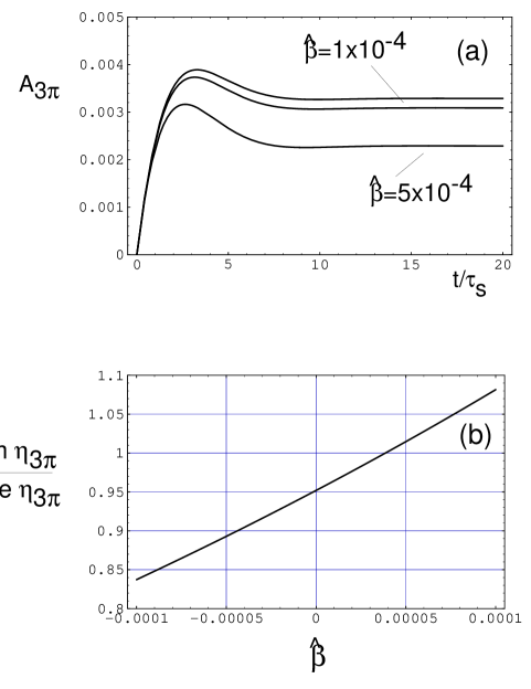
Figure 2: The time-dependent asymmetry $A_{3\pi}$ for representative choices of $\widehat{\beta}$ ($A_{3\pi}$ depends very weakly on $\widehat{\alpha},\widehat{\gamma}$). The top curve corresponds to the standard case. Also shown is the ratio ${\rm Im}\eta_{3\pi}/{\rm Re}\eta_{3\pi}=\tan(\phi-\delta\phi)$ as a function of $\widehat{\beta}$.

It is apparent from the above formulae that $A_{3\pi}$ is much more sensitive to ${\widehat{\beta}}$ that to ${\widehat{\alpha}}$ or ${\widehat{\gamma}}$. This sensitivity of $A_{3\pi}$ to ${\widehat{\beta}}$ is shown in Fig. 2(a), and that of $({\rm Im}~{}\eta_{3\pi}/{\rm Re}~{}\eta_{3\pi})$ in Fig. 2(b).

As already mentioned in Sec. 2, additional information may be obtained from $\pi^{+}\pi^{-}\pi^{0}$ decays by observing the difference between the rates for $\pi^{+}\pi^{-}\pi^{0}$ decays with $m(\pi^{+}\pi^{0})>m(\pi^{-}\pi^{0})$ and $m(\pi^{+}\pi^{0})<m(\pi^{-}\pi^{0})$ [18], represented by $O_{3\pi}^{\rm int}$ (27,28). This division of the final-state phase space into two halves is not CP-invariant, and hence enables one to measure interference between the CP-even $I_{3\pi}=2$ and CP-odd $I_{3\pi}=1$ final states. Defining

$$A_{3\pi}^{\rm int}=\frac{{\rm Tr}[O_{3\pi}^{\rm int}{\overline{\rho}(t)}]-{\rm Tr}[O_{3\pi}^{\rm int}\rho(t)]}{{\rm Tr}[O_{3\pi}^{\rm int}{\overline{\rho}(t)}]+{\rm Tr}[O_{3\pi}^{\rm int}\rho(t)]}\ ,$$ (78)

we obtain the formula

$$A_{3\pi}^{\rm int}=\frac{{\rm Re}\Delta\rho_{12}}{{\rm Re}\Sigma\rho_{12}}\ .$$ (79)

To first order in small parameters, we find

$$A_{3\pi}^{\rm int}={-e^{-\Gamma t}\left[\cos\Delta mt+{2\widehat{\alpha}\over\tan\phi}(\sin\Delta mt-(\Delta mt)\cos\Delta mt)\right]\over{|\epsilon|\over\cos\delta\phi}\left[\cos(\phi-\delta\phi)e^{-\Gamma_{L}t}+\cos(\phi+\delta\phi)e^{-\Gamma_{S}t}-2\cos\phi e^{-\Gamma t}\cos(\Delta mt-\delta\phi)\right]}$$ (80)

Note that $A_{3\pi}^{\rm int}\rightarrow\infty$ for $t\rightarrow 0$. In the CPT-conserving case this observable becomes

$$A_{3\pi}^{\rm int}\rightarrow{-e^{-\Gamma t}\cos\Delta mt\over|\epsilon|\cos\phi\left[e^{-\Gamma_{L}t}+e^{-\Gamma_{S}t}-2e^{-\Gamma t}\cos\Delta mt\right]}$$ (81)

We see that this observable is sensitive to $\widehat{\alpha}$ (see the numerator of (80)), and to $\widehat{\beta}$ via $\delta\phi$. The sensitivity to $\widehat{\alpha}$ may supplement usefully the information obtainable from the $A_{\Delta m}$ measurement discussed in section 4.5.

4.3 $A_{\rm T}$

The formula for this asymmetry, as obtained by applying the formalism of section 2, assumes the form

$$A_{\rm T}={\Delta\rho_{11}+\Delta\rho_{22}+2{\rm Re}\,\Sigma\rho_{12}\over\Sigma\rho_{11}+\Sigma\rho_{22}+2{\rm Re}\,\Delta\rho_{12}}\ ,$$ (82)

with the first-order expressions for $\Delta\rho_{11,22,12}$ and $\Sigma\rho_{11,22,12}$ given in Eqns. (54)–(LABEL:Sigmarho12^0+1). In the usual non-CPT-violating case one finds, to first order, the following exactly time-independent result

$$A_{\rm T}=4|\epsilon|\cos\phi\ ,$$ (83)

as expected [3]. In the CPT-violating case, to first order, one finds a time-dependent expression

$$A_{\rm T} = {4|\epsilon|\over\cos\delta\phi}$$

$$\left\{{e^{-\Gamma_{L}t}\cos(\phi-\delta\phi)+e^{-\Gamma_{S}t}\cos(\phi+\delta\phi)-2e^{-\Gamma t}\cos(\Delta mt-\delta\phi)\cos\phi\over e^{-\Gamma_{L}t}(1+2\widehat{\gamma})+e^{-\Gamma_{S}t}(1-2\widehat{\gamma})-2e^{-\Gamma t}[\cos\Delta mt+{2\widehat{\alpha}\over\tan\phi}(\sin\Delta mt-\Delta mt\cos\Delta mt)]}\right\}$$

which aymptotes to

$$A_{\rm T}\rightarrow{4|\epsilon|\cos(\phi-\delta\phi)\over\cos\delta\phi(1+2\widehat{\gamma})}={4|\epsilon|\cos\phi-8\widehat{\beta}\sin\phi\cos\phi\over 1+2\widehat{\gamma}}\ .$$ (85)

The sensitivity of $A_{\rm T}$ to ${\widehat{\alpha}}$ and ${\widehat{\beta}}$ are illustrated in Fig. 3(a) and Fig. 3(b), respectively. We see that the sensitivity to ${\widehat{\alpha}}$ is again less than that to ${\widehat{\beta}}$, and is restricted to $t/\tau_{s}\mathrel{\mathchoice{\vbox{\offinterlineskip\halign{$\m@th\displaystyle\hfil#\hfil$\cr<\crcr\sim\crcr} }}{\vbox{\offinterlineskip\halign{$\m@th\textstyle\hfil#\hfil$\cr<\crcr\sim\crcr} }}{\vbox{\offinterlineskip\halign{$\m@th\scriptstyle\hfil#\hfil$\cr<\crcr\sim\crcr} }}{\vbox{\offinterlineskip\halign{$\m@th\scriptscriptstyle\hfil#\hfil$\cr<\crcr\sim\crcr} }}}15$, whereas the greater sensitivity to ${\widehat{\beta}}$ persists to large $t$, as in Eq. (85), where the corresponding (utterly negligible) sensitivity to $\widehat{\gamma}$ can be inferred.

4.4 $A_{\rm CPT}$

Following the discussion in section 2, the formula for this observable, as defined by the CPLEAR Collaboration [3], is given by Eq. (30) with $f=\pi^{-}l^{+}\nu$ and $\bar{f}=\pi^{+}l^{-}\bar{\nu}$. We obtain

$$A_{\rm CPT}={\Delta\rho_{11}+\Delta\rho_{22}-2{\rm Re}\,\Sigma\rho_{12}\over\Sigma\rho_{11}+\Sigma\rho_{22}-2{\rm Re}\,\Delta\rho_{12}}\ .$$ (86)

To first order, in both the CPT-conserving and CPT-violating cases, we find

$$A_{\rm CPT}=0\ .$$ (87)

To second order, the terms in the numerator of Eq. (86) can be written most succinctly in the long-time limit. With the help of the expressions in Appendix B we obtain

$$\Delta\rho_{11}^{(2)} \rightarrow -2|\epsilon|\widehat{\gamma}\cos\phi+8|\epsilon|\widehat{\alpha}\cos\phi\sin^{2}\phi+4\widehat{\beta}\widehat{\gamma}\sin\phi\cos\phi+16\widehat{\alpha}\widehat{\beta}\sin\phi\cos^{3}\phi$$

$$\Delta\rho_{22}^{(2)} \rightarrow 2|\epsilon|\widehat{\gamma}\cos\phi-4\widehat{\beta}\widehat{\gamma}\sin\phi\cos\phi$$ (88)

$${\rm Re}\,\Sigma\rho_{12}^{(2)} \rightarrow 4|\epsilon|\widehat{\alpha}\cos\phi\sin^{2}\phi+8\widehat{\alpha}\widehat{\beta}\sin\phi\cos^{3}\phi$$

which show that in the long-time limit $A_{\rm CPT}=0$ also to second order. In fact, some algebra shows that $A_{\rm CPT}=0$ through second order for all values of $t$. This result implies that $|A_{\rm CPT}|\mathrel{\mathchoice{\vbox{\offinterlineskip\halign{$\m@th\displaystyle\hfil#\hfil$\cr<\crcr\sim\crcr} }}{\vbox{\offinterlineskip\halign{$\m@th\textstyle\hfil#\hfil$\cr<\crcr\sim\crcr} }}{\vbox{\offinterlineskip\halign{$\m@th\scriptstyle\hfil#\hfil$\cr<\crcr\sim\crcr} }}{\vbox{\offinterlineskip\halign{$\m@th\scriptscriptstyle\hfil#\hfil$\cr<\crcr\sim\crcr} }}}10^{-6}$ and thus is unobservably small.

We point out that this result is a quite distinctive signature of the modifications of the quantum mechanics proposed in Ref. [6, 15], since in the case of quantum-mechanical violation of CPT symmetry [5] there is a non-trivial change in $A_{\rm CPT}$, proportional to the CPT-violating parameters $\delta M$ and $\delta\Gamma$. Indeed, in Appendix A we obtain the following first-order asymptotic result

$$A_{\rm CPT}^{\rm QM}\rightarrow 4\sin\phi\cos\phi\,\widehat{\delta M}+2\cos^{2}\phi\,\widehat{\delta\Gamma}\ ,$$ (89)

written in terms of the scaled variables. Part of the reason for this difference is the different role played by $\delta M$ as compared to the $\beta$ parameter in the formalism of Ref. [6], as discussed in detail in Ref. [15]. In particular, there are important sign differences between the ways that $\delta M$ and $\beta$ appear in the two formalisms, that cause the suppression to second order of any quantum-mechanical-violating effects in $A_{\rm CPT}$, as opposed to the conventional quantum mechanics case.

4.5 $A_{\Delta m}$

Following Ref. [3], one can define $A_{\Delta m}$ as

$$A_{\Delta m}={R(K^{0}\rightarrow\pi^{+})+R(\bar{K}^{0}\rightarrow\pi^{-})-R(\bar{K}^{0}\rightarrow\pi^{+})-R(K^{0}\rightarrow\pi^{-})\over R(K^{0}\rightarrow\pi^{+})+R(\bar{K}^{0}\rightarrow\pi^{-})+R(\bar{K}^{0}\rightarrow\pi^{+})+R(K^{0}\rightarrow\pi^{-})}$$ (90)

in an obvious short-hand notation for the final states of the semileptonic decays, where only the pion content is shown explicitly. In the formalism of section 2, this expression becomes

$$A_{\Delta m}={2{\rm Re}\Delta\rho_{12}\over\Sigma\rho_{11}+\Sigma\rho_{22}}\ .$$ (91)

The first-order expression in the usual non-CPT violating case is

$$A_{\Delta m}=-{2e^{-\Gamma t}\cos\Delta mt\over e^{-\Gamma_{L}t}+e^{-\Gamma_{S}t}}\ ,$$ (92)

as obtained in Ref. [3]. In the CPT-violating case to first order, as Eqs. (56,57,58) show, neither $|\epsilon|$ nor $\widehat{\beta}$ come in, and we obtain

$$A_{\Delta m}=-{2e^{-\Gamma t}\left[\cos\Delta mt+{2\widehat{\alpha}\over\tan\phi}(\sin\Delta mt-\Delta mt\cos\Delta mt)\right]\over e^{-\Gamma_{L}t}(1+2\widehat{\gamma})+e^{-\Gamma_{S}t}(1-2\widehat{\gamma})}\ .$$ (93)

Since $\widehat{\gamma}$ is negligible, this observable provides an exclusive test of $\widehat{\alpha}$.

In the case of no CPT violation, the observable $A_{\Delta m}$ has a minimum for $\tan\Delta mt=-\Gamma/\Delta m\approx-{\textstyle{1\over 2}}|\Delta\Gamma|/\Delta m=-1/\tan\phi$. Since $\tan\phi\approx 1$, the minimum occurs for $(t/\tau_{s})_{\rm min}\approx 3\pi/2$. In the CPT-violating case, Eq. (93) can be rewritten as

$$A_{\Delta m}=-{2e^{-\Gamma t}C_{\Delta m}\cos(\Delta mt-\phi_{\Delta m})\over e^{-\Gamma_{L}t}(1+2\widehat{\gamma})+e^{-\Gamma_{S}t}(1-2\widehat{\gamma})}\ .$$ (94)

with

$$\tan\phi_{\Delta m}={2\widehat{\alpha}/\tan\phi\over 1-\widehat{\alpha}t|\Delta\Gamma|}\,,\qquad C_{\Delta m}={1-\widehat{\alpha}t|\Delta\Gamma|\over\cos\phi_{\Delta m}}\ .$$ (95)

Since the minimum occurs for $t|\Delta\Gamma|\sim 5$, for small values of $\widehat{\alpha}$ one can neglect the time-dependent pieces in $\phi_{\Delta m}$ and $C_{\Delta m}$. The new minimum condition for $A_{\Delta m}$ is then modified to $\tan(\Delta mt-\phi_{\Delta m})\approx-1/\tan\phi$, and thus the minimum is shifted to

$$(t/\tau_{s})_{\rm min}\approx{\textstyle{3\pi\over 2}}+4\widehat{\alpha}\ ,$$ (96)

for small values of $\widehat{\alpha}$. A similar test for $\widehat{\alpha}$ was proposed in Ref. [16], where it was based on the traditional semileptonic decay charge asymmetry parameter $\delta(t)$ [15]. However, to first order that observable depends also on $|\epsilon|$ and $\widehat{\beta}$, and as such it is not a direct test of $\widehat{\alpha}$, as opposed to the one proposed here. Figure 4 exhibits the sensitivity of $A_{\Delta m}$ to ${\widehat{\alpha}}$, including (a) the general dependence in the interference region and (b) the detailed location of the minimum as ${\widehat{\alpha}}$ is varied.

5 Regeneration

5.1 Simplified Thin-Regenerator Case

Regeneration involves the coherent scattering of a $K^{0}$ or ${\bar{K}}^{0}$ off a nuclear target, which we assume can be described using the normal framework of quantum field theory and quantum mechanics. Thus we describe it by an effective Hamiltonian which takes the form

$$\Delta H=\left(\begin{array}[]{cc}T&0\\ 0&{\overline{T}}\end{array}\right)$$ (97)

in the $(K^{0},{\bar{K}}^{0})$ basis, where

$$T=\frac{2\pi N}{m_{K}}\,{\cal M}\,,\qquad\overline{T}=\frac{2\pi N}{m_{K}}\,\overline{\cal M}$$ (98)

with ${\cal M}=\left\langle K^{0}|A|K^{0}\right\rangle$ the forward $K^{0}$-nucleus scattering amplitude (and analogously for $\overline{\cal M}$), and $N$ is the nuclear regenerator density. We can rewrite $\Delta H$ (97) in the $K_{1,2}$ basis as

$$\Delta H=\left(\begin{array}[]{cc}T+{\overline{T}}&T-{\overline{T}}\\ T-{\overline{T}}&T+{\overline{T}}\end{array}\right)\ ,$$ (99)

which can in principle be included as a contribution to $H$ in the density matrix equation:

$$\partial_{t}\rho=-i[H,\rho]+i\delta H\hskip-8.5pt/\hskip 2.0pt\rho\ ,$$ (100)

where $\delta H\hskip-8.5pt/\hskip 2.0pt$ represents the possible CPT- and QM-violating term.

It may be adequate as a first approximation to treat the regenerator as very thin, in which case we may use the impulse approximation, and the regenerator changes $\rho$ by an amount

$$\delta\rho=-i[\Delta{\cal H},\rho]\ ,$$ (101)

where

$$\Delta{\cal H}=\int dt\Delta H\ .$$ (102)

Writing

$$\rho=\left(\begin{array}[]{cc}\rho_{11}&\rho^{*}_{12}\\ \rho_{12}&\rho_{22}\end{array}\right)\ ,$$ (103)

in this approximation we obtain

$$\delta\rho=-i\Delta T\left(\begin{array}[]{cc}2i{\rm Im}\rho_{12}&-\rho_{11}+\rho_{22}\\ \rho_{11}-\rho_{22}&-2i{\rm Im}\rho_{12}\end{array}\right)\ ,$$ (104)

where

$$\Delta T\equiv\int dt(T-{\overline{T}})\ .$$ (105)

This change in $\rho$ enables the possible CPT- and QM-violating terms in (100) to be probed in a new way. Consider the idealization that the neutral $K$ beam is already in a $K_{L}$ state (Eq. (39)):

$$\rho=\rho_{L}\approx\left(\begin{array}[]{cc}1&\epsilon^{*}+B^{*}\\ \epsilon+B&|\epsilon|^{2}+C\end{array}\right)$$ (106)

where

$$B=-i2\widehat{\beta}\cos\phi\,e^{-i\phi}\qquad;\qquad C=\widehat{\gamma}-4\widehat{\beta}^{2}\cos^{2}\phi-4\widehat{\beta}|\epsilon|\sin\phi$$ (107)

Substituting Eqs. (106,107) into Eq. (104), we find that in the joint large-$t$ and impulse approximations

$$\rho+\delta\rho=\left(\begin{array}[]{cc}1+2\Delta T{\rm Im}(\epsilon+B)&\epsilon^{*}+B^{*}+i(1-|\epsilon|^{2}-C)\Delta T\\ \epsilon+B-i(1-|\epsilon|^{2}-C)\Delta T&|\epsilon|^{2}+C-2\Delta T{\rm Im}(\epsilon+B)\end{array}\right)\ .$$ (108)

We see that the usual semileptonic decay asymmetry observable

$$O_{\pi^{-}l^{+}\nu}-O_{\pi^{+}l^{-}\bar{\nu}}=\left(\begin{array}[]{cc}0&2\\ 2&0\end{array}\right)\qquad,$$ (109)

which measures ${\rm Re}(\epsilon+B)$ in the case without the regenerator, receives no contribution from the regenerator (i.e., $\Delta T$ cancels out in the sum of the off-diagonal elements). On the other hand, there is a new contribution to the value of $R_{2\pi}=R(K_{L}\rightarrow 2\pi)={\rm Tr}[O_{2\pi}\rho]=\rho_{22}$, namely

$$R_{2\pi}=|\epsilon|^{2}+\widehat{\gamma}-4\widehat{\beta}^{2}\cos^{2}\phi-4\widehat{\beta}|\epsilon|\sin\phi-2\Delta T{\rm Im}(\epsilon+B)\ .$$ (110)

The quantity ${\rm Im}(\epsilon+B)$ was not accessible directly to the observable $R_{2\pi}$ in the absence of a regenerator. Theoretically, the phases of $\epsilon$ and $B$ (107) are fixed, i.e.,

$${\rm Im}(\epsilon+B)=-|\epsilon|{\sin(\phi-\delta\phi)\over\cos\delta\phi}=-|\epsilon|\sin\phi-2\widehat{\beta}\cos^{2}\phi\ .$$ (111)

Nevertheless, this phase prediction should be checked, so the regenerator makes a useful addition to the physics programme.

The above analysis is oversimplified, since the impulse approximation may not be sufficiently precise, and the neutral $K$ beam is not exactly in a $K_{L}$ state. Moreover, the result in Eq. (108) is valid only at the time the beam emerges from the regenerator. However, this simple example may serve to illustrate the physics interest of measurements using a regenerator. We next generalize the analysis to include a general neutral $K$ beam encountering a thin regenerator, with the full time dependence after leaving the regenerator.

5.2 Detailed Regenerator Tests

To make contact with the overall discussion in this paper, we envision the following scenario:

(i) Pure $K^{0},\bar{K}^{0}$ beams are produced at time $t=0$, corresponding to initial density matrices $\rho_{0}$ and $\bar{\rho}_{0}$, respectively.

(ii) These beams are described by density matrices $\rho(t)$ and $\bar{\rho}(t)$, and evolve with time as described in Section 2, until a time $t=t_{r}$ where they are described by $\rho(t_{r})$ and $\bar{\rho}(t_{r})$.

(iii) At $t=t_{r}$ a thin regenerator is encountered. In our thin-regenerator approximation (described in the previous subsection), at $t=t_{r}$ suddenly the density matrices receive an additional contribution $\delta\rho(t_{r})$ and $\delta\bar{\rho}(t_{r})$, according to Eq. (104).

(iv) For $\tau=t-t_{r}\geq 0$, the beams are described by density matrices $\rho^{r}(\tau)$ and $\bar{\rho}^{r}(\tau)$, which again evolve as described in Section 2, but this time with initial conditions $\rho^{r}(0)=\rho(t_{r})+\delta\rho(t_{r})$ and $\bar{\rho}^{r}(0)=\bar{\rho}(t_{r})+\delta\bar{\rho}(t_{r})$.

In this context, we consider two kinds of tests. In a CPLEAR-like scenario, the identity of the beam is known irrespective of the presence of the regenerator, and thus a measurement of $A^{r}_{2\pi}(\tau)$, i.e., $A_{2\pi}$ after the thin regenerator is traversed, appears feasible. The second test is reminiscent of the Fermilab experiments, where the experimental setup is such that $t_{r}\gg\tau_{S}$, and the beam is in a $K_{L}$ state. After the regenerator is traversed one then measures $R_{2\pi}$ in the interference region.

Before embarking on elaborate calculations, we should perhaps quantify our “thin-regenerator” criterion. For the impulse approximation to be valid, $\delta\rho$ in Eq. (104) should not change $\rho$ by too much. Since the entries in $\rho$ are typically ${\cal O}(10^{-3})$ or smaller, we should demand that $\Delta T$ be a reasonably small number. Let us estimate $\Delta T=\int dt(T-\bar{T})$. Assuming ${\cal M}-\overline{\cal M}\sim 1/m_{\pi}$ and relativistic kaons we obtain

$$\Delta T\approx{\textstyle{1\over 30}}\,{\rm thickness}\,[{\rm cm}]\ {\rm density}\,[{\rm g/cm^{3}}]\ ,$$ (112)

and thus a “thin” regenerator should have a thickness $\mathrel{\mathchoice{\vbox{\offinterlineskip\halign{$\m@th\displaystyle\hfil#\hfil$\cr<\crcr\sim\crcr} }}{\vbox{\offinterlineskip\halign{$\m@th\textstyle\hfil#\hfil$\cr<\crcr\sim\crcr} }}{\vbox{\offinterlineskip\halign{$\m@th\scriptstyle\hfil#\hfil$\cr<\crcr\sim\crcr} }}{\vbox{\offinterlineskip\halign{$\m@th\scriptscriptstyle\hfil#\hfil$\cr<\crcr\sim\crcr} }}}{\cal O}(1\,{\rm cm})$. This estimate appears reasonable when considering that in the 2 ns or so that the beams are usually observed (about $20\tau_{S}$), they travel $\sim 60\,{\rm cm}$. Such a regenerator could conceivably be installed in an upgraded CPLEAR experiment. In the Fermilab E731 [19] and E773 [20, 21] experiments the regenerators used are much thicker, and the validity of our approximation is unclear.

5.2.1 $A^{r}_{2\pi}$

We start with $A^{r}_{2\pi}=\Delta\rho^{r}_{22}/\Sigma\rho^{r}_{22}$, where e.g., $\Delta\rho^{r}_{22}(\tau)$ is given by $\rho_{22}(\tau)$ in Eqns. (45,51) with $\rho(0)\rightarrow\Delta\rho^{r}(0)=\Delta\rho(t_{r})+\delta(\Delta\rho)(t_{r})$, and $\delta(\Delta\rho)$ given in Eq. (104) with $\rho\rightarrow\Delta\rho$. We obtain

$$\Delta\rho^{r}_{22}(\tau) = \Biggl{\{}[\Delta\rho_{22}(t_{r})-2\Delta T{\rm Im}\Delta\rho_{12}(t_{r})]-\widehat{\gamma}\,[\Delta\rho_{11}(t_{r})+2\Delta T{\rm Im}\Delta\rho_{12}(t_{r})]$$ (113)

$$-2|\epsilon|\,{\cos(\phi+\delta\phi+\Delta\phi_{12})\over\cos\delta\phi}\,|\Delta\rho^{r}_{12}(0)|\Biggr{\}}e^{-\Gamma_{S}\tau}$$

$$+\widehat{\gamma}\,[\Delta\rho_{11}(t_{r})+2\Delta T{\rm Im}\Delta\rho_{12}(t_{r})]e^{-\Gamma_{L}\tau}$$

$$+{2|\epsilon|\over\cos\delta\phi}|\Delta\rho^{r}_{12}(0)|e^{-\Gamma\tau}\cos(\Delta m\tau-\phi-\delta\phi-\Delta\phi_{12})\ ,$$

$$\Sigma\rho^{r}_{22}(\tau) = \Biggl{\{}[\Sigma\rho_{22}(t_{r})-2\Delta T{\rm Im}\Sigma\rho_{12}(t_{r})]-\widehat{\gamma}\,[\Sigma\rho_{11}(t_{r})+2\Delta T{\rm Im}\Sigma\rho_{12}(t_{r})]$$ (114)

$$-2|\epsilon|\,{\cos(\phi+\delta\phi+\Sigma\phi_{12})\over\cos\delta\phi}\,|\Sigma\rho^{r}_{12}(0)|\Biggr{\}}e^{-\Gamma_{S}\tau}$$

$$+\widehat{\gamma}\,[\Sigma\rho_{11}(t_{r})+2\Delta T{\rm Im}\Sigma\rho_{12}(t_{r})]e^{-\Gamma_{L}\tau}$$

$$+{2|\epsilon|\over\cos\delta\phi}|\Sigma\rho^{r}_{12}(0)|e^{-\Gamma\tau}\cos(\Delta m\tau-\phi-\delta\phi-\Sigma\phi_{12})\ ,$$

where we have defined the phases $\Delta\phi_{12}$ and $\Sigma\phi_{12}$ through

$$\Delta\rho^{r}_{12}(0) = \left|\Delta\rho_{12}(t_{r})-i\Delta T[\Delta\rho_{11}(t_{r})-\Delta\rho_{22}(t_{r})]\right|e^{i\Delta\phi_{12}}\ ,$$ (115)

$$\Sigma\rho^{r}_{12}(0) = \left|\Sigma\rho_{12}(t_{r})-i\Delta T[\Sigma\rho_{11}(t_{r})-\Sigma\rho_{22}(t_{r})]\right|e^{i\Sigma\phi_{12}}\ .$$ (116)

In these expressions, the “initial-condition” input matrices $\Delta\rho(t_{r})$ and $\Sigma\rho(t_{r})$ are obtained from Eqns. (54)–(LABEL:Sigmarho12^0+1) by inserting $t=t_{r}$. We obtain a rather complicated result, which, in addition to the CPT-violating parameters, also depends on $\Delta T$ and $t_{r}$. To illustrate the behavior of $A^{r}_{2\pi}$ let us consider two limiting cases: $t_{r}\ll\tau_{S}$ and $t_{r}\gg\tau_{S}$. For a regenerator very close to the origin ($t_{r}\ll\tau_{S}$) we basically have $\Delta\rho(t_{r})\approx\Delta\rho(0)$ and $\Sigma\rho(t_{r})\approx\Sigma\rho(0)$, as in Eq. (36), and we obtain

$$\Delta\rho^{r}_{22}(\tau) \rightarrow 2|\epsilon|\,{\cos(\phi+\delta\phi)\over\cos\delta\phi}\,e^{-\Gamma_{S}\tau}-{2|\epsilon|\over\cos\delta\phi}e^{-\Gamma\tau}\cos(\Delta m\tau-\phi-\delta\phi)\ ,$$ (117)

$$\Sigma\rho^{r}_{22}(\tau) \rightarrow (1-\widehat{\gamma})e^{-\Gamma_{S}\tau}+\widehat{\gamma}e^{-\Gamma_{L}\tau}\ .$$ (118)

Neglecting $\widehat{\gamma}$ we find

$$A^{r}_{2\pi}(\tau)\rightarrow{2|\epsilon|\over\cos\delta\phi}\left\{\cos(\phi+\delta\phi)-e^{{1\over 2}(\Gamma_{S}-\Gamma_{L})\tau}\cos(\Delta m\tau-\phi-\delta\phi)\right\}$$ (119)

Thus, when the regenerator is placed near the production point the effects of $\Delta T$ drop out, and the result without a regenerator is recovered (see Eq. (61) dropping $\widehat{\gamma}$ and all second-order terms).

Of more interest is the case of a regenerator placed in the asymptotic region ($t_{r}\gg\tau_{S}$). In this case the expressions for $\Delta\rho(t_{r})$ and $\Sigma\rho(t_{r})$ simplify considerably, through first order:

$$\Delta\rho_{11}(t_{r})\rightarrow{2|\epsilon|\cos(\phi-\delta\phi)\over\cos\delta\phi}$$

(120)

Inserting these limiting expressions (and taking $\widehat{\gamma}=0$) we obtain

$$\Delta\rho^{r}_{22}(\tau) \rightarrow -2|\epsilon|\,{\cos(\phi+\delta\phi+\Delta\phi_{12})\over\cos\delta\phi}\,|\Delta\rho^{r}_{12}(0)|e^{-\Gamma_{S}\tau}$$ (121)

$$+{2|\epsilon|\over\cos\delta\phi}|\Delta\rho^{r}_{12}(0)|e^{-\Gamma\tau}\cos(\Delta m\tau-\phi-\delta\phi-\Delta\phi_{12})\ ,$$

$$\Sigma\rho^{r}_{22}(\tau) \rightarrow \Biggl{\{}2\Delta T|\epsilon|{\sin(\phi-\delta\phi)\over\cos\delta\phi}-2|\epsilon|\,{\cos(\phi+\delta\phi+\Sigma\phi_{12})\over\cos\delta\phi}\,|\Sigma\rho^{r}_{12}(0)|\Biggr{\}}e^{-\Gamma_{S}\tau}$$ (122)

$$+{2|\epsilon|\over\cos\delta\phi}|\Sigma\rho^{r}_{12}(0)|e^{-\Gamma\tau}\cos(\Delta m\tau-\phi-\delta\phi-\Sigma\phi_{12})\ ,$$

and thus

$$A^{r}_{2\pi}(\tau) \rightarrow {|\Delta\rho^{r}_{12}(0)|\over|\Sigma\rho^{r}_{12}(0)|}\left\{-\cos(\phi+\delta\phi+\Delta\phi_{12})+e^{{1\over 2}(\Gamma_{S}-\Gamma_{L})\tau}\cos(\Delta m\tau-\phi-\delta\phi-\Delta\phi_{12})\right\}$$ (123)

$$/\Biggl{\{}\left[{\Delta T\over|\Sigma\rho^{r}_{12}(0)|}\sin(\phi-\delta\phi)-\cos(\phi+\delta\phi+\Sigma\phi_{12})\right]$$

$$\qquad\qquad\qquad\qquad+e^{{1\over 2}(\Gamma_{S}-\Gamma_{L})\tau}\cos(\Delta m\tau-\phi-\delta\phi-\Sigma\phi_{12})\Biggr{\}}$$

with

$$\Delta\rho^{r}_{12}(0) \rightarrow \left|-i\Delta T{2|\epsilon|\cos(\phi-\delta\phi)\over\cos\delta\phi}\right|e^{i\Delta\phi_{12}}\Rightarrow\Delta\phi_{12}=-{\textstyle{\pi\over 2}}\ ,$$ (124)

$$\Sigma\rho^{r}_{12}(0) \rightarrow \left|{|\epsilon|\over\cos\delta\phi}e^{i(\delta\phi-\phi)}-i\Delta T\right|e^{i\Sigma\phi_{12}}\ .$$ (125)

The result in Eq. (123) reveals a large shift ($\Delta\phi_{12}=-{\textstyle{\pi\over 2}}$) in the interference pattern relative to the case of no regenerator. According to our estimate of $\Delta T$ in Eq. (112), it would appear that $\Delta T\gg|\epsilon|$ is a case of interest to consider. In this limit, $\Delta T$ drops out from the $A^{r}_{2\pi}$ observable, $\Delta\phi_{12}=\Sigma\phi_{12}=-{\textstyle{\pi\over 2}}$, and

$$A^{r}_{2\pi}(\tau)\rightarrow 2|\epsilon|{\cos(\phi-\delta\phi)\over\cos\delta\phi}\,{\sin(\phi+\delta\phi)+e^{{1\over 2}(\Gamma_{S}-\Gamma_{L})\tau}\sin(\Delta m\tau-\phi-\delta\phi)\over\sin(\phi+\delta\phi)-\sin(\phi-\delta\phi)+e^{{1\over 2}(\Gamma_{S}-\Gamma_{L})\tau}\sin(\Delta m\tau-\phi-\delta\phi)}$$ (126)

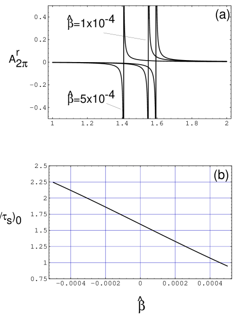
Figure 5: The time-dependent asymmetry $A^{r}_{2\pi}(\tau)$ in the presence of a thin regenerator placed far from the production point, as a function of the time $\tau$ after leaving the regenerator, for representative choices of $\widehat{\beta}$ ($A^{r}_{2\pi}(\tau)$ is rather insensitive to $\widehat{\alpha},\widehat{\gamma}$, which are set to zero). The right-most curve corresponds to the standard case. Also shown (b) is the position of the (first) zero in $A^{r}_{2\pi}(\tau)$ as a function of $\widehat{\beta}$.

The time-dependence of $A^{r}_{2\pi}(\tau)$ is shown in Fig. 5 from which it is apparent that $A^{r}_{2\pi}(\tau)$ is basically flat except for values of $\tau$ for which $\sin(\Delta m\tau-\phi-\delta\phi)=0$. This occurs for $(\tau/\tau_{S})_{0}\approx 2(n\pi+{\pi\over 4}+\delta\phi)$, a result which is plotted against $\widehat{\beta}$ (for $n=0$) also in Fig. 5. We note that for increasingly larger values of $n$, the structure in the curves becomes narrower and therefore much less sensitive to $\widehat{\beta}$, with the first zero ($n=0$) possibly being the only observable one.

5.2.2 $R_{2\pi}$

The observable $R_{2\pi}=R(K\rightarrow 2\pi)$ has traditionally been the focus of CP violation studies. Because the detector is physically located a distance away from the source of the neutral kaons, most of the $K_{S}$ component of the beam decays away, and one is basically sensitive only to the $K_{L}\rightarrow 2\pi$ decays. To study also the interesting interference region, a regenerator is inserted in the path of the $K_{L}$ particles right before they reach the detector, so that $K_{S}$ particles are regenerated and interference studies are possible. Unfortunately, the regenerator complicates the physics somewhat. To simplify the problem, let us first consider the case of a pure $K^{0}$ beam whose decay products can be detected from the instant of production (not unlike in the CPLEAR experiment). We will address the effect of the regenerator in the next subsection.

In our formalism, the $R_{2\pi}$ observable corresponds to the operator ${\cal O}_{2\pi}$ in (21), which gives

$$R_{2\pi}(t)=\rho_{22}(t)\ .$$ (127)

Through second order, the corresponding expression is obtained from Eqs. (45,51,230) by inserting $\rho_{11}(0)=\rho_{22}(0)=\rho_{12}(0)=1$. In the case of standard quantum-mechanical CP violation, one obtains

$$R_{2\pi}(t)=c_{S}\,e^{-\Gamma_{S}t}+c_{L}\,e^{-\Gamma_{L}t}+2c_{I}\,e^{-\Gamma t}\cos(\Delta mt-\phi)\ ,$$ (128)

where to second order the $c_{S},c_{L},c_{I}$ coefficients are given by:

$$c_{S} = 1-2|\epsilon|\cos\phi+|\epsilon|^{2}(1+2\cos 2\phi+t|\Delta\Gamma|)$$ (129)

$$c_{L} = |\epsilon|^{2}$$ (130)

$$c_{I} = |\epsilon|-2|\epsilon|^{2}\cos\phi$$ (131)

It is then apparent that to the order calculated: $c_{I}^{2}=c_{S}c_{L}=|\epsilon|^{2}$. Violations of this relation would indicate departures from standard quantum mechanics, which can be parametrized by [22]

$$\zeta=1-{c_{I}\over\sqrt{c_{S}c_{L}}}\ .$$ (132)

In our quantum-mechanical-violating framework we expect $\zeta\not=0$. Indeed, we obtain

$$c_{S} = 1-\widehat{\gamma}-2|\epsilon|{\cos(\phi+\delta\phi)\over\cos\delta\phi}$$ (133)

$$c_{L} = \widehat{\gamma}+\widehat{\gamma}^{2}+|\epsilon|^{2}{\cos(\phi-2\delta\phi)\over\cos\phi\cos^{2}\delta\phi}-2|\epsilon|\widehat{\gamma}{\cos(\phi-\delta\phi)\over\cos\delta\phi}$$ (134)

$$c_{I} = {|\epsilon|\over\cos\delta\phi}$$ (135)

where only terms relevant to the computation of $\zeta$ to second order have been kept (note that $\widehat{\alpha}$ does not contribute to $\zeta$ to the order calculated). Also, in this case the general relation in Eq. (128) gets modified by a phase shift in the interference term $\phi\rightarrow\phi+\delta\phi$. Using these expressions we obtain

$${c^{2}_{I}\over c_{S}c_{L}}={{|\epsilon|^{2}/\cos^{2}\delta\phi}\over\widehat{\gamma}(1-4|\epsilon|\cos\phi)+|\epsilon|^{2}{\cos(\phi-2\delta\phi)\over\cos\phi\cos^{2}\delta\phi}}\approx{1\over{\widehat{\gamma}\over|\epsilon|^{2}}+{\cos(\phi-2\delta\phi)\over\cos\phi}}$$ (136)

and thus

$$\zeta\approx{1\over 2}\left[1-{1\over{\widehat{\gamma}\over|\epsilon|^{2}}+{\cos(\phi-2\delta\phi)\over\cos\phi}}\right]\approx{\widehat{\gamma}\over 2|\epsilon|^{2}}-{2\widehat{\beta}\over|\epsilon|}\sin\phi\ ,$$ (137)

where the second form holds for small values of $\widehat{\gamma}/|\epsilon|^{2}$ and $\delta\phi\approx-2\widehat{\beta}\cos\phi/|\epsilon|$. The parameter $\zeta$ has been measured to be $\zeta^{\rm exp}=0.03\pm 0.02$ [23]. Setting $\widehat{\beta}=0$ one obtains $\widehat{\gamma}\approx(3\pm 2)\times 10^{-7}$ [22]. More generally, the dependence of $\zeta$ on $\widehat{\beta}$ and $\widehat{\gamma}$ is shown in Fig. 6, along with the present experimental limits on $\zeta$.

5.2.3 $R^{r}_{2\pi}$

Let us now turn to the $R^{r}_{2\pi}=\rho^{r}_{22}(\tau)$ observable in the presence of a thin regenerator. Here $\rho^{r}_{22}(\tau)$ is given to first order by Eqns. (45,51) with $\rho(0)\rightarrow\rho^{r}(0)=\rho(t_{r})+\delta\rho(t_{r})$, and $\delta\rho$ given in Eqn. (104). We obtain

$$R^{r}_{2\pi}(\tau) = \Biggl{\{}[\rho_{22}(t_{r})-2\Delta T{\rm Im}\rho_{12}(t_{r})]-\widehat{\gamma}\,[\rho_{11}(t_{r})+2\Delta T{\rm Im}\rho_{12}(t_{r})]$$ (138)

$$-2|\epsilon|\,{\cos(\phi+\delta\phi+\phi_{12})\over\cos\delta\phi}\,|\rho^{r}_{12}(0)|\Biggr{\}}e^{-\Gamma_{S}\tau}$$

$$+\widehat{\gamma}\,[\rho_{11}(t_{r})+2\Delta T{\rm Im}\rho_{12}(t_{r})]e^{-\Gamma_{L}\tau}$$

$$+{2|\epsilon|\over\cos\delta\phi}|\rho^{r}_{12}(0)|e^{-\Gamma\tau}\cos(\Delta m\tau-\phi-\delta\phi-\phi_{12})\ ,$$

where

$$\rho^{r}_{12}(0)=\left|\rho_{12}(t_{r})-i\Delta T[\rho_{11}(t_{r})-\rho_{22}(t_{r})]\right|e^{i\phi_{12}}\ .$$ (139)

As we discussed above, the initial condition matrix $\rho(t_{r})$ is simply $\rho_{L}$, namely

$$\rho(t_{r})=\left(\begin{array}[]{cc}1+\widehat{\gamma}-2|\epsilon|\cos\phi+4\widehat{\beta}\sin\phi\cos\phi&(|\epsilon|+i2{\widehat{\beta}}\cos\phi)e^{i\phi}\\ (|\epsilon|-i2{\widehat{\beta}}\cos\phi)e^{-i\phi}&|\epsilon|^{2}+{\widehat{\gamma}}-4{\widehat{\beta}}^{2}\cos^{2}\phi-4{\widehat{\beta}}|\epsilon|\sin\phi\end{array}\right)\ .$$ (140)

Note that at the instant the beam leaves the regenerator ($\tau=0$), we obtain $R^{r}_{2\pi}(0)=\rho_{22}^{r}(0)=\rho_{22}(t_{r})-2\Delta T{\rm Im}\rho_{12}(t_{r})$ which, after inserting $\rho(t_{r})$ from Eq. (140), agrees with the result derived above in Eq. (110) where no time dependence after leaving the regenerator was considered.

In the interference region the expression for $R_{2\pi}$ simplifies considerably: we keep only the term proportional to $e^{-\Gamma\tau}$,

$$R^{\rm int}_{2\pi}(\tau)={2|\epsilon|\over\cos\delta\phi}|\rho^{r}_{12}(0)|e^{-\Gamma\tau}\cos(\Delta m\tau-\phi-\delta\phi-\phi_{12})\ ,$$ (141)

with

$$\rho^{r}_{12}(0)\approx\left|{|\epsilon|\over\cos\delta\phi}e^{i(\delta\phi-\phi)}-i\Delta T\right|e^{i\phi_{12}}\ .$$ (142)

In this case we again see that the regenerator introduces a shift in the interference pattern and modifies its overall magnitude, even in the absence of CPT violation. In the limit in which $\Delta T\gg|\epsilon|$, $|\rho_{12}^{r}(0)|\rightarrow\Delta T$, $\phi_{12}\rightarrow-{\textstyle{\pi\over 2}}$ and

$$R_{2\pi}^{\rm int}(\tau)\rightarrow{2|\epsilon|\Delta T\over\cos\delta\phi}e^{-\Gamma\tau}\cos(\Delta m\tau-\phi-\delta\phi+{\textstyle{\pi\over 2}})\ ,$$ (143)

which exhibits a large phase shift and a distinctive linear dependence on $\Delta T$, which is a nice signature. Moreover, the result still allows a determination of the CPT-violating parameter $\beta$, through $\delta\phi$ (53).

We now address the $\zeta$ parameter in the presence of a regenerator. Let us first start with the case of standard quantum mechanics, where we expect $\zeta$ to vanish. Looking back at Eqs. (129,130,131), we see that (to the order calculated) the $\zeta=0$ relation amounts to $[c^{(1)}_{I}]^{2}=c^{(0)}_{S}c^{(2)}_{2}$, where the orders at which the relevant contributions appear have been indicated. In the case of a regenerator, the time dependence of $\rho^{r}_{22}(\tau)$ is the same as that of $\rho_{22}(t)$, the only difference being in the coefficients which depend on different initial-condition matrices ($\rho^{r}(0)$ versus $\rho(0)$). To make our result more general, we will keep this initial-condition matrix unspecified. Using Eqns. (45,51,230) we then get

$$c^{(0)}_{S} = \rho_{22}(0)$$ (144)

$$c^{(2)}_{L} = \rho_{11}(0)|\epsilon|^{2}$$ (145)

$$c^{(1)}_{I} = |\rho_{12}(0)||\epsilon|$$ (146)

and therefore

$$\zeta_{\rm QM}=1-{c_{I}\over\sqrt{c_{S}c_{L}}}=1-{|\rho_{12}(0)|\over\sqrt{\rho_{11}(0)\rho_{22}(0)}}=0\ ,$$ (147)

where we have used the fact that a pure quantum-mechanical ($2\times 2$) density matrix has zero determinant ($\det\rho(0)=\rho_{11}(0)\rho_{22}(0)-|\rho_{12}(0)|^{2}$). This result applies immediately to the regenerator case where a particular form of $\rho(0)$ is used, namely: $\rho^{r}_{11}(0)\approx 1$, $\rho^{r}_{22}(0)\approx|\epsilon|^{2}+2\Delta T|\epsilon|\sin\phi$, $|\rho^{r}_{12}(0)|^{2}\approx|\epsilon|^{2}+2\Delta T|\epsilon|\sin\phi$, which indeed satisfy $\det\rho^{r}(0)=0$.

We now repeat the exercise in our quantum-mechanics-violating framework, where we obtain

$$c^{(0+1)}_{S} = \rho_{22}(0)-\rho_{11}(0)\widehat{\gamma}-2|\epsilon||\rho_{12}(0)|\,{\cos(\phi+\delta\phi+\phi_{12})\over\cos\delta\phi}$$ (148)

$$c^{(1+2)}_{L} = \rho_{11}(0)\widehat{\gamma}+\rho_{22}(0)\widehat{\gamma}^{2}+\rho_{11}(0)|\epsilon|^{2}\,{\cos(\phi-2\delta\phi)\over\cos\phi\cos^{2}\delta\phi}-2|\epsilon|\widehat{\gamma}|\rho_{12}(0)|\,{\cos(\phi-\delta\phi-\phi_{12})\over\cos\delta\phi}$$

$$c^{(1)}_{I} = {|\epsilon|\over\cos\delta\phi}|\rho_{12}(0)|$$ (150)

which entail

$${c^{2}_{I}\over c_{S}c_{L}} = {|\epsilon|^{2}\over\cos^{2}\delta\phi}|\rho_{12}(0)|^{2}$$

$$/\Biggl{\{}\rho_{11}(0)\rho_{22}(0)\widehat{\gamma}+[\rho^{2}_{22}(0)-\rho^{2}_{11}(0)]\widehat{\gamma}^{2}+\rho_{11}(0)\rho_{22}(0)|\epsilon|^{2}{\cos(\phi-2\delta\phi)\over\cos\phi\cos^{2}\delta\phi}$$

$$-{2|\epsilon|\widehat{\gamma}\over\cos\delta\phi}|\rho_{12}(0)|[\rho_{22}(0)\cos(\phi-\delta\phi-\phi_{12})+\rho_{11}(0)\cos(\phi+\delta\phi+\phi_{12})]\Biggr{\}}$$

This expression can be most easily interpreted in the limit of interest, $\Delta T\gg|\epsilon|$, where the initial condition matrix $\rho^{r}(0)$ reduces to

$$\rho^{r}_{11}(0) \approx 1\ ,$$ (152)

$$\rho^{r}_{22}(0) \approx \widehat{\gamma}+2\Delta T|\epsilon|\,{\sin(\phi-\delta\phi)\over\cos\delta\phi}+|\epsilon|^{2}\,{\cos(\phi-2\delta\phi)\over\cos\phi\cos^{2}\delta\phi}\ ,$$ (153)

$$|\rho^{r}_{12}(0)|^{2} \approx 2\Delta T|\epsilon|\,{\sin(\phi-\delta\phi)\over\cos\delta\phi}+{|\epsilon|^{2}\over\cos^{2}\delta\phi}\ .$$ (154)

Note that the source of quantum mechanical decoherence is given by

$$\det\rho^{r}(0)\approx\widehat{\gamma}-2|\epsilon|^{2}\,{\sin(\phi-\delta\phi)\sin\delta\phi\over\cos\phi\cos^{2}\delta\phi}\approx\widehat{\gamma}\ .$$ (155)

With these expressions for $\rho^{r}(0)$ one obtains for the numerator and denominator of Eq. (LABEL:zeta_r)

$$c^{2}_{I} \approx {|\epsilon|^{2}\over\cos^{2}\delta\phi}\left[2\Delta T|\epsilon|\,{\sin(\phi-\delta\phi)\over\cos\delta\phi}\right]$$ (156)

$$c_{S}c_{L} \approx 2\Delta T|\epsilon|\,{\sin(\phi-\delta\phi)\over\cos\delta\phi}\left[\widehat{\gamma}+|\epsilon|^{2}\,{\cos(\phi-2\delta\phi)\over\cos\phi\cos^{2}\delta\phi}\right]$$ (157)

and thus the regenerator effects ($\Delta T$) drop out, and the expressions without a regenerator in Eqs. (136,137) are recovered, i.e., $\zeta_{r}=\zeta$. This result also implies that the experimental limits on $\zeta$ that are derived in the presence of a regenerator can be directly applied to our expression for $\zeta$, as assumed in the previous subsection.

We note that, although the study of $\zeta$ alone, in tests using a regenerator [22], does not seem to add anything to the discussion of the possible breakdown of quantum-mechanical coherence within our framework, individual terms in the expression (138) for $R_{2\pi}^{r}(\tau)$ depend linearly on the regenerator density via $\Delta T$, and the dependence on the non-quantum-mechanical parameters is different from the no-regenerator case, so the regenerator is able to provide interesting new probes of our framework. In this respect, experimental tests of CPT-symmetry within quantum mechanics suggested earlier [24], using arrays of regenerators, find also a natural application within our quantum-mechanics-violating framework.

5.2.4 $A^{r}_{\rm CPT}$

In Sec. 4.4 we showed that there is no contribution to the $A_{\rm CPT}$ observable up to second order. One may wonder whether the introduction of a regenerator could change this result. To this end we compute $A_{\rm CPT}^{r}$, which is defined as in Eq. (86) but with the $\Delta\rho,\Sigma\rho$ matrices replaced by the $\Delta\rho^{r},\Sigma\rho^{r}$ matrices. Expressions for the latter are complicated, as exhibited explicitly in the previous subsections. However, the expression for $A_{\rm CPT}^{r}$ simplifies considerably when calculated consistently through first order only, since many of the entries in the input matrices $\Delta\rho(t_{r}),\Sigma\rho(t_{r})$ need to be evaluated only to zeroth order. After some algebra we obtain

$$A_{\rm CPT}^{r}(\tau)=2\Delta T{[e^{-\Gamma t_{r}}\sin(\Delta mt_{r})](e^{-\Gamma_{L}\tau}-e^{-\Gamma_{S}\tau})+[e^{-\Gamma_{L}t_{r}}-e^{-\Gamma_{S}t_{r}}]e^{-\Gamma\tau}\sin\Delta(m\tau)\over e^{-\Gamma_{L}t_{r}}\,e^{-\Gamma_{L}\tau}+e^{-\Gamma_{S}t_{r}}\,e^{-\Gamma_{S}\tau}+2e^{-\Gamma t_{r}}\,e^{-\Gamma\tau}\cos(\Delta m\tau+\Delta mt_{r})}\ ,$$ (158)

which for $\tau\gg\tau_{S}$ asymptotes to

$$A_{\rm CPT}^{r}(\tau)\rightarrow 2\Delta T\,e^{[-{1\over 2}(\Gamma_{S}-\Gamma_{L})t_{r}]}\sin(\Delta mt_{r})\ .$$ (159)

Thus we see that all dependence on the CP- ($|\epsilon|$) and CPT- ($\alpha,\beta,\gamma$) violating parameters drops out, which confirms the result obtained without a regenerator. The novelty is that $A_{\rm CPT}^{r}$ is nonetheless non-zero, and proportional to $\Delta T$. This result is interesting, but not unexpected since the matter in the regenerator scatters $K^{0}$ differently from $\bar{K}^{0}$ (98). Formally, this is expressed by the fact that the regenerator Hamiltonian in Eq. (99) is proportional to $\sigma_{1}$, therefore does not commute with the CPT operator, and so violates CPT. That is, the regenerator is a CPT-violating environment, although completely within standard quantum mechanics.

6 Indicative Bounds on CPT-Violating Parameters

The formulae derived above are ready to be used in fits to the experimental data. A complete analysis requires a detailed understanding of all the statistical and systematic errors, and their correlations, which goes beyond the scope of this paper [25]. Here we restrict ourselves to indications of the magnitudes of the bounds that are likely to be obtained from such an analysis.

The parameter $\widehat{\alpha}$ can be constrained by observing that the overall size of the interference term in $A_{2\pi}$ (61) does not differ significantly from the standard result [see also Fig. 1(a)]. The relevant dependence on $\widehat{\alpha}$ comes at second order through $\Delta X_{3}$, which is given in Eq. (64). From this expression we can see that the dominant term is the third one, i.e., $(-2|\epsilon|\widehat{\alpha}/\cos\delta\phi)t|\Delta\Gamma|\cos(\Delta mt-\phi-\delta\phi)$, which is enhanced relative to the other terms because of the $t|\Delta\Gamma|$ factor. The dominant interference term through second order is then

$$-{2|\epsilon|\over\cos\delta\phi}\,[1+\widehat{\alpha}t|\Delta\Gamma|]\,e^{{1\over 2}(\Gamma_{S}-\Gamma_{L})t}\cos(\Delta mt-\phi-\delta\phi)\ .$$ (160)

For our indicative purposes, we assume that the size of the interference term is within 5% of the standard result for observations in the range $t/\tau_{S}\mathrel{\mathchoice{\vbox{\offinterlineskip\halign{$\m@th\displaystyle\hfil#\hfil$\cr<\crcr\sim\crcr} }}{\vbox{\offinterlineskip\halign{$\m@th\textstyle\hfil#\hfil$\cr<\crcr\sim\crcr} }}{\vbox{\offinterlineskip\halign{$\m@th\scriptstyle\hfil#\hfil$\cr<\crcr\sim\crcr} }}{\vbox{\offinterlineskip\halign{$\m@th\scriptscriptstyle\hfil#\hfil$\cr<\crcr\sim\crcr} }}}10$. Since $\widehat{\alpha}>0$ and the overall factor $(1/\cos\delta\phi)\approx 1$ (see below), we require $\widehat{\alpha}t|\Delta\Gamma|\mathrel{\mathchoice{\vbox{\offinterlineskip\halign{$\m@th\displaystyle\hfil#\hfil$\cr<\crcr\sim\crcr} }}{\vbox{\offinterlineskip\halign{$\m@th\textstyle\hfil#\hfil$\cr<\crcr\sim\crcr} }}{\vbox{\offinterlineskip\halign{$\m@th\scriptstyle\hfil#\hfil$\cr<\crcr\sim\crcr} }}{\vbox{\offinterlineskip\halign{$\m@th\scriptscriptstyle\hfil#\hfil$\cr<\crcr\sim\crcr} }}}0.05$ [16], i.e.,

$$\widehat{\alpha}\mathrel{\mathchoice{\vbox{\offinterlineskip\halign{$\m@th\displaystyle\hfil#\hfil$\cr<\crcr\sim\crcr} }}{\vbox{\offinterlineskip\halign{$\m@th\textstyle\hfil#\hfil$\cr<\crcr\sim\crcr} }}{\vbox{\offinterlineskip\halign{$\m@th\scriptstyle\hfil#\hfil$\cr<\crcr\sim\crcr} }}{\vbox{\offinterlineskip\halign{$\m@th\scriptscriptstyle\hfil#\hfil$\cr<\crcr\sim\crcr} }}}5.0\times 10^{-3}\ ,\qquad\alpha\mathrel{\mathchoice{\vbox{\offinterlineskip\halign{$\m@th\displaystyle\hfil#\hfil$\cr<\crcr\sim\crcr} }}{\vbox{\offinterlineskip\halign{$\m@th\textstyle\hfil#\hfil$\cr<\crcr\sim\crcr} }}{\vbox{\offinterlineskip\halign{$\m@th\scriptstyle\hfil#\hfil$\cr<\crcr\sim\crcr} }}{\vbox{\offinterlineskip\halign{$\m@th\scriptscriptstyle\hfil#\hfil$\cr<\crcr\sim\crcr} }}}3.7\times 10^{-17}\,{\rm GeV}\ .$$ (161)

This is to be compared to the order of magnitude ${\cal O}((\Lambda_{\rm QCD}~{}{\rm or}~{}m_{s})^{2}/M_{Pl})\mathrel{\mathchoice{\vbox{\offinterlineskip\halign{$\m@th\displaystyle\hfil#\hfil$\cr<\crcr\sim\crcr} }}{\vbox{\offinterlineskip\halign{$\m@th\textstyle\hfil#\hfil$\cr<\crcr\sim\crcr} }}{\vbox{\offinterlineskip\halign{$\m@th\scriptstyle\hfil#\hfil$\cr<\crcr\sim\crcr} }}{\vbox{\offinterlineskip\halign{$\m@th\scriptscriptstyle\hfil#\hfil$\cr<\crcr\sim\crcr} }}}10^{-19}\,{\rm GeV}$ which is of theoretical interest in the neutral kaon system.

The simplest way to constrain the parameter ${\widehat{\beta}}$ involves the observables $R_{2\pi}$ and $A_{2\pi}$, which differ from the standard results at first order in $\widehat{\beta}$, as seen in Fig. 1(b). This new contribution can affect the overall size of the interference pattern and shift its phase relative to the superweak phase $\phi$, as seen in equations (61) and (141). It is easy to check that the shift in phase $\delta\phi$ is sufficiently small for any possible change in the overall size of the interference pattern (due to $\delta\phi$) to be negligible, e.g., $|\delta\phi|<2^{\circ}$ implies a change in the size by $<6\times 10^{-4}$. There are two independent sets of data that give information on $\delta\phi$ : (i) the Particle Data Group compilation [1] which fits NA31, E731 and earlier data, and (ii) more recent data from the E773 Collaboration [20, 21]. New data from the CPLEAR collaboration are discussed elsewhere [25]. In each case, both the superweak phase $\phi$ and the $K\rightarrow\pi^{+}\pi^{-}$ interference phase $\phi_{+-}$ are measured, and the corresponding values of $\delta\phi=\phi_{+-}-\phi$ are extracted :

$$\delta\phi=(-0.71\pm 0.95)^{\circ}~{}\cite[cite]{[\@@bibref{}{pdg}{}{}]},\qquad\delta\phi=(-0.84\pm 1.42)^{\circ}~{}\cite[cite]{[\@@bibref{}{E773}{}{}]}\ .$$ (162)

Combining these independent measurements in quadrature, we find $\delta\phi=(-0.75\pm 0.79)^{\circ}$, corresponding to

$$\widehat{\beta}=(2.0\pm 2.2)\times 10^{-5}\ ,\qquad\beta=(1.5\pm 1.6)\times 10^{-19}\,{\rm GeV}\ ,$$ (163)

to be compared with the earlier bound $|{\widehat{\beta}}|\mathrel{\mathchoice{\vbox{\offinterlineskip\halign{$\m@th\displaystyle\hfil#\hfil$\cr<\crcr\sim\crcr} }}{\vbox{\offinterlineskip\halign{$\m@th\textstyle\hfil#\hfil$\cr<\crcr\sim\crcr} }}{\vbox{\offinterlineskip\halign{$\m@th\scriptstyle\hfil#\hfil$\cr<\crcr\sim\crcr} }}{\vbox{\offinterlineskip\halign{$\m@th\scriptscriptstyle\hfil#\hfil$\cr<\crcr\sim\crcr} }}}6\times 10^{-5}$ obtained in ref. [16] by demanding $|\delta\phi|\mathrel{\mathchoice{\vbox{\offinterlineskip\halign{$\m@th\displaystyle\hfil#\hfil$\cr<\crcr\sim\crcr} }}{\vbox{\offinterlineskip\halign{$\m@th\textstyle\hfil#\hfil$\cr<\crcr\sim\crcr} }}{\vbox{\offinterlineskip\halign{$\m@th\scriptstyle\hfil#\hfil$\cr<\crcr\sim\crcr} }}{\vbox{\offinterlineskip\halign{$\m@th\scriptscriptstyle\hfil#\hfil$\cr<\crcr\sim\crcr} }}}2^{\circ}$. As expected from Fig. 1, the indicative bound (163) on $|{\widehat{\beta}}|$ is considerably more restrictive than that (161) on $|{\widehat{\alpha}}|$. Alternatively, one may bound $\widehat{\beta}$ by considering the relationship (see e.g., [21])

$$|m_{K^{0}}-m_{\bar{K}^{0}}|\approx 2\Delta m{|\eta_{+-}|\over\sin\Phi_{\rm sw}}\,|\Phi_{+-}-\Phi_{\rm sw}+{\textstyle{1\over 3}}\Delta\Phi|\ ,$$ (164)

where $\Delta\Phi=\Phi_{00}-\Phi_{+-}$. In our framework, up to $\epsilon^{\prime}/\epsilon$ effects, $\Delta\Phi=0$, $\Phi_{\rm sw}=\phi$, $\Phi_{+-}=\phi+\delta\phi$, $|\eta_{+-}|=|\epsilon|/\cos\delta\phi\approx|\epsilon|$, and thus

$$|m_{K^{0}}-m_{\bar{K}^{0}}|\approx 2\Delta m{|\epsilon||\delta\phi|\over\sin\phi}\approx 2|\beta|\ .$$ (165)

The E773 Collaboration has determined that [21] $|m_{K^{0}}-m_{\bar{K}^{0}}|/m_{K^{0}}<7.5\times 10^{-19}$ at the 90% CL, and thus it follows that $|\widehat{\beta}|<2.6\times 10^{-5}$, $|\beta|<1.9\times 10^{-19}\,{\rm GeV}$. This result is consistent with that in Eq. (163).

Table 1: Compilation of indicative bounds on CPT-violating parameters and their source.

Source		Indicative bound
$R_{2\pi},A_{2\pi}$		$\widehat{\alpha}<5.0\times 10^{-3}$
$R_{2\pi},A_{2\pi}$		$\widehat{\beta}=(2.0\pm 2.2)\times 10^{-5}$
$|m_{K^{0}}-m_{\bar{K}^{0}}|$		$\widehat{\beta}<2.6\times 10^{-5}$
$R_{2\pi}$		$\widehat{\gamma}\mathrel{\mathchoice{\vbox{\offinterlineskip\halign{$\m@th\displaystyle\hfil#\hfil$\cr<\crcr\sim\crcr} }}{\vbox{\offinterlineskip\halign{$\m@th\textstyle\hfil#\hfil$\cr<\crcr\sim\crcr} }}{\vbox{\offinterlineskip\halign{$\m@th\scriptstyle\hfil#\hfil$\cr<\crcr\sim\crcr} }}{\vbox{\offinterlineskip\halign{$\m@th\scriptscriptstyle\hfil#\hfil$\cr<\crcr\sim\crcr} }}}5\times 10^{-7}$
$\zeta$		${\widehat{\gamma}\over 2|\epsilon|^{2}}-{2\widehat{\beta}\over|\epsilon|}\sin\phi=0.03\pm 0.02$
Positivity		$\widehat{\alpha}>\widehat{\beta}^{2}/\widehat{\gamma}_{\rm max}\sim(10^{3}\widehat{\beta})^{2}$

 

The $\widehat{\gamma}$ parameter has the peculiar property of appearing in the observables at first order, but without being accompanied by a similar first-order term proportional to $|\epsilon|$ (as is the case for $\widehat{\beta}$). In fact, if corresponding terms exist, they are proportional to $|\epsilon|^{2}$. This means that large deviations from the usual results would occur unless $\widehat{\gamma}\mathrel{\mathchoice{\vbox{\offinterlineskip\halign{$\m@th\displaystyle\hfil#\hfil$\cr<\crcr\sim\crcr} }}{\vbox{\offinterlineskip\halign{$\m@th\textstyle\hfil#\hfil$\cr<\crcr\sim\crcr} }}{\vbox{\offinterlineskip\halign{$\m@th\scriptstyle\hfil#\hfil$\cr<\crcr\sim\crcr} }}{\vbox{\offinterlineskip\halign{$\m@th\scriptscriptstyle\hfil#\hfil$\cr<\crcr\sim\crcr} }}}|\epsilon|^{2}$. This result is exemplified in Fig. 1(c), from which we conclude that $\widehat{\gamma}<10^{-5}$. In Ref. [16] $\widehat{\gamma}\mathrel{\mathchoice{\vbox{\offinterlineskip\halign{$\m@th\displaystyle\hfil#\hfil$\cr<\crcr\sim\crcr} }}{\vbox{\offinterlineskip\halign{$\m@th\textstyle\hfil#\hfil$\cr<\crcr\sim\crcr} }}{\vbox{\offinterlineskip\halign{$\m@th\scriptstyle\hfil#\hfil$\cr<\crcr\sim\crcr} }}{\vbox{\offinterlineskip\halign{$\m@th\scriptscriptstyle\hfil#\hfil$\cr<\crcr\sim\crcr} }}}0.1|\epsilon|^{2}$ was obtained. However, since $|\epsilon^{\prime}/\epsilon|\sim 10^{-3}$ effects have been neglected, we conclude conservatively that

$$\widehat{\gamma}\mathrel{\mathchoice{\vbox{\offinterlineskip\halign{$\m@th\displaystyle\hfil#\hfil$\cr<\crcr\sim\crcr} }}{\vbox{\offinterlineskip\halign{$\m@th\textstyle\hfil#\hfil$\cr<\crcr\sim\crcr} }}{\vbox{\offinterlineskip\halign{$\m@th\scriptstyle\hfil#\hfil$\cr<\crcr\sim\crcr} }}{\vbox{\offinterlineskip\halign{$\m@th\scriptscriptstyle\hfil#\hfil$\cr<\crcr\sim\crcr} }}}\left|{\epsilon^{\prime}\over\epsilon}\right||\epsilon|\sim 10^{-6}\,,\qquad\gamma\mathrel{\mathchoice{\vbox{\offinterlineskip\halign{$\m@th\displaystyle\hfil#\hfil$\cr<\crcr\sim\crcr} }}{\vbox{\offinterlineskip\halign{$\m@th\textstyle\hfil#\hfil$\cr<\crcr\sim\crcr} }}{\vbox{\offinterlineskip\halign{$\m@th\scriptstyle\hfil#\hfil$\cr<\crcr\sim\crcr} }}{\vbox{\offinterlineskip\halign{$\m@th\scriptscriptstyle\hfil#\hfil$\cr<\crcr\sim\crcr} }}}7\times 10^{-20}\,{\rm GeV}\ .$$ (166)

We can also study the combined effects of $\widehat{\beta}$ and $\widehat{\gamma}$ on the $\zeta$ parameter in Eq. (137), which reads

$${\widehat{\gamma}\over 2|\epsilon|^{2}}-{2\widehat{\beta}\over|\epsilon|}\sin\phi=0.03\pm 0.02\ .$$ (167)

The combined bounds on both parameters can be read off Fig. 6, which makes clearly the point that a combined fit is essential to obtain the true bounds on the CPT-violating parameters. Note that the bounds on $\widehat{\beta}$ (163) and $\widehat{\gamma}$ (166) derived above are consistent with those that follow from Eq. (167) (see Fig. 6).

Let us close this section with a remark concerning the positivity constraints in Eq. (14): $\alpha>0,\gamma>0$, and $\alpha\gamma>\beta^{2}$. The data are not yet sufficient to conclude anything about the sign of the $\alpha$ and $\gamma$ parameters. The third constraint implies

$$\widehat{\alpha}>{\widehat{\beta}^{2}\over\widehat{\gamma}}>{\widehat{\beta}^{2}\over\widehat{\gamma}_{\rm max}}\sim(10^{3}\,\widehat{\beta})^{2}\ .$$ (168)

Thus, if $\beta$ is observable, say $\widehat{\beta}\sim 10^{-5}$, then $\widehat{\alpha}>10^{-4}$ should be observable too. A compilation of all these indicative bounds and their sources is given in Table 1.

7 Comment on Two-Particle Decay Correlations

Interesting further tests of quantum mechanics and CPT symmetry can be devised by exploiting initial-state correlations due to the production of a pair of neutral kaons in a pure quantum-mechanical state, e.g., via $e^{+}e^{-}\rightarrow\phi\rightarrow K^{0}{\bar{K}}^{0}$. In this case, the initial state may be represented by [26]

$$\left|{\bf k}~{};~{}{\bf-k}\right\rangle={\textstyle{1\over\sqrt{2}}}\left[\left|K^{0}({\bf k})~{};~{}{\bar{K}}^{0}({\bf-k})\right\rangle-\left|{\bar{K}}^{0}({\bf k})~{};~{}K^{0}({\bf-k})\right\rangle\right]$$ (169)

At subsequent times $t=t_{1}$ for particle $1$ and $t=t_{2}$ for particle $2$, the joint probability amplitude is given in conventional quantum mechanics by

$$\left|{\bf k},~{}t_{1}~{};~{}{\bf-k},~{}t_{2}\right\rangle\equiv e^{-iH({\bf k})t_{1}}e^{-iH({\bf-k})t_{2}}\left|{\bf k}~{};~{}{\bf-k}\right\rangle$$ (170)

Thus the temporal evolution of the two-particle state is completely determined by the one-particle variables (OPV) contained in $H$.

Tests of quantum mechanics and CPT symmetry in $\phi$ decays have recently been discussed [17] in a conjectured extension of the formalism of [6, 15], in which the density matrix of the two-particle system was hypothesized to be described completely in terms of such one-particle variables (OPV): namely $H$ and $(\alpha,\beta,\gamma)$. It was pointed out that this OPV hypothesis had several striking consequences, including apparent violations of energy conservation and angular momentum.

As we have discussed above [27], the only known theoretical framework in which eq. (2) has been derived is that of a non-critical string approach to string theory, in which (i) energy is conserved in the mean as a consequence of the renormalizability of the world-sheet $\sigma$-model, but (ii) angular momentum is not necessarily conserved [15, 9], as this is not guaranteed by renormalizability and is known to be violated in some toy backgrounds [27], though we cannot exclude the possibility that it may be conserved in some particular backgrounds. Therefore, we are not concerned that [17] find angular momentum non-conservation in their hypothesized OPV approach. However, the absence of energy conservation in their approach leads us to the conclusion that irreducible two-particle parameters must be introduced into the evolution of the two-particle density matrix. The appearance of such non-local parameters does not concern us, as the string is intrinsically non-local in target space, and this fact plays a key role in our model calculations of contributions to $\delta H\hskip-8.5pt/\hskip 2.0pt$. The justification and parametrization of such irreducible two-particle effects goes beyond the scope of this paper, and we plan to study this subject in more detail in due course.

8 Conclusions

We have derived in this paper approximate expressions for a complete set of neutral kaon decay observables ($2\pi,3\pi,\pi\ell\nu)$ which can be used to constrain parameters characterising CPT violation in a formalism, motivated by ideas about quantum gravity and string theory, that incorporates a possible microscopic loss of quantum coherence by treating the neutral kaon as an open quantum-mechanical system. Our explicit expressions are to second order in the small CPT-violating parameters $\alpha,\beta,\gamma$, and our systematic procedure for constructing analytic approximations may be extended to any desired level of accuracy. Our formulae may be used to obtain indicative upper bounds

$$\alpha\mathrel{\mathchoice{\vbox{\offinterlineskip\halign{$\m@th\displaystyle\hfil#\hfil$\cr<\crcr\sim\crcr} }}{\vbox{\offinterlineskip\halign{$\m@th\textstyle\hfil#\hfil$\cr<\crcr\sim\crcr} }}{\vbox{\offinterlineskip\halign{$\m@th\scriptstyle\hfil#\hfil$\cr<\crcr\sim\crcr} }}{\vbox{\offinterlineskip\halign{$\m@th\scriptscriptstyle\hfil#\hfil$\cr<\crcr\sim\crcr} }}}4\times 10^{-17}\,{\rm GeV}\,,\quad|\beta|\mathrel{\mathchoice{\vbox{\offinterlineskip\halign{$\m@th\displaystyle\hfil#\hfil$\cr<\crcr\sim\crcr} }}{\vbox{\offinterlineskip\halign{$\m@th\textstyle\hfil#\hfil$\cr<\crcr\sim\crcr} }}{\vbox{\offinterlineskip\halign{$\m@th\scriptstyle\hfil#\hfil$\cr<\crcr\sim\crcr} }}{\vbox{\offinterlineskip\halign{$\m@th\scriptscriptstyle\hfil#\hfil$\cr<\crcr\sim\crcr} }}}3\times 10^{-19}\,{\rm GeV}\,,\quad\gamma\mathrel{\mathchoice{\vbox{\offinterlineskip\halign{$\m@th\displaystyle\hfil#\hfil$\cr<\crcr\sim\crcr} }}{\vbox{\offinterlineskip\halign{$\m@th\textstyle\hfil#\hfil$\cr<\crcr\sim\crcr} }}{\vbox{\offinterlineskip\halign{$\m@th\scriptstyle\hfil#\hfil$\cr<\crcr\sim\crcr} }}{\vbox{\offinterlineskip\halign{$\m@th\scriptscriptstyle\hfil#\hfil$\cr<\crcr\sim\crcr} }}}7\times 10^{-20}\,{\rm GeV}\,,$$ (171)

which are comparable with the order of magnitude $\sim 10^{-19}\,{\rm GeV}$ which theory indicates might be attained by such CPT- and quantum-mechanics- violating parameters. Detailed fits to recent CPLEAR experimental data are reported elsewhere [25].

We have not presented explicit expressions for the case where the deviation $|\epsilon^{\prime}/\epsilon|\mathrel{\mathchoice{\vbox{\offinterlineskip\halign{$\m@th\displaystyle\hfil#\hfil$\cr<\crcr\sim\crcr} }}{\vbox{\offinterlineskip\halign{$\m@th\textstyle\hfil#\hfil$\cr<\crcr\sim\crcr} }}{\vbox{\offinterlineskip\halign{$\m@th\scriptstyle\hfil#\hfil$\cr<\crcr\sim\crcr} }}{\vbox{\offinterlineskip\halign{$\m@th\scriptscriptstyle\hfil#\hfil$\cr<\crcr\sim\crcr} }}}10^{-3}$ from pure superweak CP violation is non-negligible, but our methods can easily be extended to this case. They can also be used to obtain more specific expressions for experiments with a regenerator, if desired. The extension of the formalism of Ref. [6] to correlated $K^{0}\bar{K}^{0}$ systems produced in $\phi$ decay, as at DA$\Phi$NE [4], involves the introduction of two-particle variables, which lies beyond the scope of this paper.

Table 2: Qualitative comparison of predictions for various observables in CPT-violating theories beyond (QMV) and within (QM) quantum mechanics. Predictions either differ ($\not=$) or agree ($=$) with the results obtained in conventional quantum-mechanical CP violation. Note that these frameworks can be qualitatively distinguished via their predictions for $A_{\rm T}$, $A_{\rm CPT}$, $A_{\Delta m}$, and $\zeta$.

Process	QMV	QM
$A_{2\pi}$	$\not=$	$\not=$
$A_{3\pi}$	$\not=$	$\not=$
$A_{\rm T}$	$\not=$	$=$
$A_{\rm CPT}$	$=$	$\not=$
$A_{\Delta m}$	$\not=$	$=$
$\zeta$	$\not=$	$=$

 

As mentioned in the main text, in Appendix A we have obtained formulae for all observables in the case of CPT violation within standard quantum mechanics. In the case of $A^{\rm QM}_{2\pi}$ and $A^{\rm QM}_{3\pi}$ one can “mimic” the results from standard CP violation with suitable choices of the CPT-violating parameters ($\delta M=0$, $\widehat{\delta\Gamma}\rightarrow-2|\epsilon|/\cos\phi$). However, this possibility is experimentally excluded because of the large value it entails for the $A_{\rm CPT}$ observable. In passing we showed that the $\zeta$ parameter vanishes since no violations of quantum mechanics are allowed. In analogy with Sec. 6, we also obtained indicative bounds on the CPT-violating parameters. In Table 2 we list all the observables and make a qualitative comparison between them and conventional quantum-mechanical CP violation. We see that the quantum-mechanical (QM) and quantum-mechanics-violating (QMV) CPT-violating frameworks can be qualitatively distinguished by their predictions for $A_{\rm T}$, $A_{\rm CPT}$, $A_{\Delta m}$, and $\zeta$.

We close by reiterating that the neutral kaon system is the best microscopic laboratory for testing quantum mechanics and CPT symmetry. We believe that violations of these two fundamental principles, if present at all, are likely to be linked, and have proposed a formalism that can be used to explore systematically this hypothesis, which is motivated by ideas about quantum gravity and string theory. Our understanding of these difficult issues is so incomplete that we cannot calculate the sensitivity which would be required to reveal modifications of quantum mechanics or a violation of CPT. Hence we cannot promise success in any experimental search for such phenomena. However, we believe that both the theoretical and experimental communities should be open to their possible appearance.

Appendix A CPT Violation in the Quantum-Mechanical Density Matrix Formalism for Neutral Kaons

In this appendix we review the density matrix formalism for neutral kaons and CPT violation within the conventional quantum-mechanical framework [5, 15]. The time evolution of a generic density matrix is determined in this case by the usual quantum Liouville equation

$$\partial_{t}\rho=-i(H\rho-\rho H^{\dagger})\ .$$ (172)

The conventional phenomenological Hamiltonian for the neutral kaon system contains hermitian (mass) and antihermitian (decay) components:

$$H=\left(\begin{array}[]{cc}(M+{\textstyle{1\over 2}}\delta M)-{\textstyle{1\over 2}}i(\Gamma+{\textstyle{1\over 2}}\delta\Gamma)&M_{12}^{*}-{\textstyle{1\over 2}}i\Gamma_{12}^{*}\\ M_{12}-{\textstyle{1\over 2}}i\Gamma_{12}&(M-{\textstyle{1\over 2}}\delta M)-{\textstyle{1\over 2}}i(\Gamma-{\textstyle{1\over 2}}\delta\Gamma)\end{array}\right)\ ,$$ (173)

in the ($K^{0}$, ${\bar{K}}^{0}$) basis. The ${\delta}M$ and ${\delta}{\Gamma}$ terms violate CPT [5]. As in Ref. [6], we define components of $\rho$ and $H$ by

$$\rho\equiv{\textstyle{1\over 2}}\rho_{\alpha}\sigma_{\alpha}\qquad;\qquad H\equiv{\textstyle{1\over 2}}h_{\alpha}\sigma_{\alpha}\qquad;\qquad\alpha=0,1,2,3$$ (174)

in a Pauli $\sigma$-matrix representation : the ${\rho_{\alpha}}$ are real, but the $h_{\beta}$ are complex. The CPT transformation is represented by

$${\rm CPT}\left|K^{0}\right\rangle=e^{i\theta}\left|{\bar{K}}^{0}\right\rangle,\qquad{\rm CPT}\left|{\bar{K}}^{0}\right\rangle=e^{-i\theta}\left|K^{0}\right\rangle\ ,$$ (175)

for some phase ${\theta}$, which is represented in our matrix formalism by

$${\rm CPT}\equiv\left(\begin{array}[]{c}0\qquad e^{i\theta}\\ e^{-i\theta}\qquad 0\end{array}\right)\ .$$ (176)

Since this matrix is a linear combination of ${\sigma}_{1,2}$, CPT invariance of the phenomenological Hamiltonian, $H$ = $({\rm CPT})^{-1}H({\rm CPT})$, clearly requires that $H$ contain no term proportional to ${\sigma}_{3}$, i.e., $h_{3}$ = $0$ so that ${\delta}M$ = ${\delta}{\Gamma}$ = $0$.

Conventional quantum-mechanical evolution is represented by $\partial_{t}\rho_{\alpha}=H_{{\alpha}{\beta}}{\rho_{\beta}}$, where, in the ($K^{0}$, ${\bar{K}}^{0}$) basis and allowing for the possibility of CPT violation,

$$H_{\alpha\beta}\equiv\left(\begin{array}[]{rrrr}{\rm Im}h_{0}&{\rm Im}h_{1}&{\rm Im}h_{2}&{\rm Im}h_{3}\\ {\rm Im}h_{1}&{\rm Im}h_{0}&-{\rm Re}h_{3}&{\rm Re}h_{2}\\ {\rm Im}h_{2}&{\rm Re}h_{3}&{\rm Im}h_{0}&-{\rm Re}h_{1}\\ {\rm Im}h_{3}&-{\rm Re}h_{2}&{\rm Re}h_{1}&{\rm Im}h_{0}\end{array}\right)\ .$$ (177)

We note that the real parts of the matrix $h$ are antisymmetric, whilst its imaginary parts are symmetric. Now is an appropriate time to transform to the $K_{1,2}={\textstyle{1\over\sqrt{2}}}(K^{0}\mp{\bar{K}}^{0})$ basis, corresponding to $\sigma_{1}\leftrightarrow\sigma_{3}$, $\sigma_{2}\leftrightarrow-\sigma_{2}$, in which $H_{\alpha\beta}$ becomes

$$H_{\alpha\beta}=\left(\begin{array}[]{cccc}-\Gamma&-{\textstyle{1\over 2}}\delta\Gamma&-{\rm Im}\Gamma_{12}&-{\rm Re}\Gamma_{12}\\ -{\textstyle{1\over 2}}\delta\Gamma&-\Gamma&-2{\rm Re}M_{12}&-2{\rm Im}M_{12}\\ -{\rm Im}\Gamma_{12}&2{\rm Re}M_{12}&-\Gamma&-\delta M\\ -{\rm Re}\Gamma_{12}&-2{\rm Im}M_{12}&\delta M&-\Gamma\end{array}\right)\ .$$ (178)

The corresponding equations of motion for the components of $\rho$ in the $K_{1,2}$ basis are [as above we neglect ${\rm Im}\Gamma_{12}$ contributions]

$$\dot{\rho}_{11} = -\Gamma_{L}\rho_{11}-2{\rm Re}\,[({\rm Im}M_{12}+{\textstyle{1\over 4}}\delta\Gamma+{\textstyle{i\over 2}}\delta M)\rho_{12}]\,,$$ (179)

$$\dot{\rho}_{12} = -(\Gamma+i\Delta m)\rho_{12}+({\rm Im}M_{12}-{\textstyle{1\over 4}}\delta\Gamma-{\textstyle{i\over 2}}\delta M)\rho_{11}-({\rm Im}M_{12}+{\textstyle{1\over 4}}\delta\Gamma-{\textstyle{i\over 2}}\delta M)\rho_{22},$$

$$\dot{\rho}_{22} = -\Gamma_{S}\rho_{22}+2{\rm Re}\,[({\rm Im}M_{12}-{\textstyle{1\over 4}}\delta\Gamma+{\textstyle{i\over 2}}\delta M)\rho_{12}]\ .$$ (181)

One can readily verify that ${\rho}$ decays at large $t$ to

$$\rho\sim e^{-\Gamma_{L}t}\left(\begin{array}[]{cc}1&\epsilon^{*}+\delta^{*}\\ \epsilon+\delta&|\epsilon+\delta|^{2}\end{array}\right)\ ,$$ (182)

which has a vanishing determinant, thus corresponding to a pure long-lived mass eigenstate $K_{L}$. The CP-violating parameter ${\epsilon}$ and the CPT-violating parameter $\delta$ are given as above, namely

$$\epsilon=\frac{{\rm Im}M_{12}}{{\textstyle{1\over 2}}|\Delta\Gamma|+i\Delta m}\ ,\qquad\delta=-{\textstyle{1\over 2}}\frac{{\textstyle{1\over 2}}\delta\Gamma+i\delta M}{{\textstyle{1\over 2}}|\Delta\Gamma|+i\Delta m}\ .$$ (183)

Conversely, in the short-$t$ limit a $K_{S}$ state is represented by

$$\rho\sim e^{-\Gamma_{S}t}\left(\begin{array}[]{cc}|\epsilon-\delta|^{2}&\epsilon-\delta\\ \epsilon^{*}-\delta^{*}&1\end{array}\right)\ ,$$ (184)

which also has zero determinant. Note that the relative signs of the $\delta$ terms have reversed: this is the signature of CPT violation in the conventional quantum-mechanical formalism. Note that the density matrices (182,184) correspond to the state vectors

$$\left|K_{L}\right\rangle \propto (1+\epsilon-\delta)\left|K^{0}\right\rangle-(1-\epsilon+\delta)\left|{\bar{K}}^{0}\right\rangle$$ (185)

$$\left|K_{S}\right\rangle \propto (1+\epsilon+\delta)\left|K^{0}\right\rangle+(1-\epsilon-\delta)\left|{\bar{K}}^{0}\right\rangle$$ (186)

and are both pure, as should be expected in conventional quantum mechanics, even if CPT is violated.

As above, we solve the differential equations in perturbation theory in $|\epsilon|$ and the new parameters

$$\widehat{\delta M}\equiv{\delta M\over|\Delta\Gamma|}\ ,\qquad\widehat{\delta\Gamma}\equiv{\delta\Gamma\over|\Delta\Gamma|}\ .$$ (187)

The zeroth order results for the $\rho_{ij}$ are the same as those in Eqs. (44,45,46), namely

$$\rho^{(0)}_{11}(t) = \rho_{11}(0)\,e^{-\Gamma_{L}t}\ ,$$ (188)

$$\rho^{(0)}_{22}(t) = \rho_{22}(0)\,e^{-\Gamma_{S}t}\ ,$$ (189)

$$\rho^{(0)}_{12}(t) = \rho_{12}(0)\,e^{-(\Gamma+i\Delta mt)}\ .$$ (190)

The first-order results for the density matrix elements are:

$$\rho_{11}^{(1)} = -2|X^{\prime}||\rho_{12}(0)|\left[e^{-\Gamma_{L}t}\cos(\phi-\phi_{X^{\prime}}-\phi_{12})-e^{-\Gamma t}\cos(\Delta mt+\phi-\phi_{X^{\prime}}-\phi_{12})\right]$$ (191)

$$\rho_{22}^{(1)} = -2|X||\rho_{12}(0)|\left[e^{-\Gamma_{S}t}\cos(\phi+\phi_{X}+\phi_{12})-e^{-\Gamma t}\cos(\Delta mt-\phi-\phi_{X}-\phi_{12})\right]$$ (192)

$$\rho_{12}^{(1)} = \rho_{11}(0)|X|e^{-i(\phi+\phi_{X})}\left[e^{-\Gamma_{L}t}-e^{-(\Gamma+i\Delta m)t}\right]+\rho_{22}(0)|X^{\prime}|e^{i(\phi-\phi_{X^{\prime}})}\left[e^{-\Gamma_{S}t}-e^{-(\Gamma+i\Delta m)t}\right]$$

where the two complex constants $X$ and $X^{\prime}$ are defined by:

$$X = |\epsilon|-{\textstyle{1\over 2}}\cos\phi\,\widehat{\delta\Gamma}+i\cos\phi\,\widehat{\delta M}\,,\qquad\tan\phi_{X}={\cos\phi\,\widehat{\delta M}\over|\epsilon|-{\textstyle{1\over 2}}\cos\phi\,\widehat{\delta\Gamma}}\ ,$$ (194)

$$X^{\prime} = |\epsilon|+{\textstyle{1\over 2}}\cos\phi\,\widehat{\delta\Gamma}+i\cos\phi\,\widehat{\delta M}\,,\qquad\tan\phi_{X^{\prime}}={\cos\phi\,\widehat{\delta M}\over|\epsilon|+{\textstyle{1\over 2}}\cos\phi\,\widehat{\delta\Gamma}}\ .$$ (195)

For future reference, we note the special case that occurs when $\delta M=0$ and $|\epsilon|=0$, namely

$$\delta\Gamma>0: \phi_{X}=\pi,\quad\phi_{X^{\prime}}=0\ ;$$ (196)

$$\delta\Gamma<0: \phi_{X}=0,\quad\phi_{X^{\prime}}=\pi\ .$$ (197)

With the results for $\rho$ through first order, and inserting the appropriate initial conditions (36), we can immediately write down the expressions for the various observables discussed in Sec. 4. For $A_{2\pi}$ we obtain

$$A^{\rm QM}_{2\pi}(t)={2|X|\cos(\phi+\phi_{X})-2|X|e^{{1\over 2}(\Gamma_{S}-\Gamma_{L})t}\cos(\Delta mt-\phi-\phi_{X})\over 1+e^{(\Gamma_{S}-\Gamma_{L})t}\,|X|^{2}}\ ,$$ (198)

where in the denominator we have also included the non-negligible second-order contributions to $\Sigma\rho_{22}^{(2)}$. From this expression it is interesting to note that one can mimic the standard CP-violating result for $A_{2\pi}$ in Eq. (68) by setting $|\epsilon|\rightarrow 0$ and making the following choices for the CPT-violating parameters

$${\rm mimic\ CP\ violation:}\qquad\qquad\delta M=0,\qquad\widehat{\delta\Gamma}\rightarrow-{2|\epsilon|\over\cos\phi}\ ,$$ (199)

which give $|X|\rightarrow|\epsilon|$ and $\phi_{X}=0$. For the $A_{3\pi}$ observable we find

$$A^{\rm QM}_{3\pi}(t)=2|X^{\prime}|\cos(\phi-\phi_{X^{\prime}})-2e^{-{1\over 2}(\Gamma_{S}-\Gamma_{L})t}\left[{\rm Re}\eta_{3\pi}\cos\Delta mt-{\rm Im}\eta_{3\pi}\sin\Delta mt\right]\ ,$$ (200)

with

$${\rm Re}\eta_{3\pi}=|X^{\prime}|\cos(\phi-\phi_{X^{\prime}}),\quad{\rm Im}\eta_{3\pi}=|X^{\prime}|\sin(\phi-\phi_{X^{\prime}})\ ,$$ (201)

that is

$${{\rm Im}\eta_{3\pi}\over{\rm Re}\eta_{3\pi}}=\tan(\phi-\phi_{X^{\prime}})\ .$$ (202)

Here we also note that the standard CP-violating result is obtained for the choices of parameters in Eq. (199) which give $|X^{\prime}|\rightarrow|\epsilon|$ and $\phi_{X^{\prime}}=\pi$, since $\tan(\phi-\pi)=\tan\phi$.

For the observable $A_{\rm T}$, we obtain the following exactly time-independent first-order expression

$$A^{\rm QM}_{\rm T}=2|X^{\prime}|\cos(\phi-\phi_{X^{\prime}})+2|X|\cos(\phi+\phi_{X})=4|\epsilon|\cos\phi\ ,$$ (203)

which is identical to the case of no CPT violation. In the case of $A_{\rm CPT}$ we find

$$A^{\rm QM}_{\rm CPT}(t)={A_{1}(e^{-\Gamma_{L}t}-e^{-\Gamma_{S}t})-2e^{-\Gamma t}A_{2}\sin\Delta mt\over e^{-\Gamma_{L}t}+e^{-\Gamma_{S}t}-2e^{-\Gamma t}\cos\Delta mt}\ ,$$ (204)

with

$$\!\!\!\!\!\!\!\!\!\!\!\!\!\!\!\!\!\!A_{1}=2|X^{\prime}|\cos(\phi-\phi_{X^{\prime}})-2|X|\cos(\phi+\phi_{X})=4\sin\phi\cos\phi\,\widehat{\delta M}+2\cos^{2}\phi\,\widehat{\delta\Gamma}$$ (205)

$$\!\!\!\!\!\!\!\!\!\!\!\!\!\!\!\!\!\!A_{2}=-2|X^{\prime}|\sin(\phi-\phi_{X^{\prime}})+2|X|\sin(\phi+\phi_{X})=4\cos^{2}\phi\,\widehat{\delta M}-2\sin\phi\cos\phi\,\widehat{\delta\Gamma}$$ (206)

Note that $|\epsilon|$ drops out of the expression for $A_{\rm CPT}$ as it should. In the long-time limit we obtain

$$A^{\rm QM}_{\rm CPT}\rightarrow 4\sin\phi\cos\phi\,\widehat{\delta M}+2\cos^{2}\phi\,\widehat{\delta\Gamma}\ .$$ (207)

Since the dynamical equations determining the density matrix do not manifestly possess the mimicking symmetry in Eq. (199), one expects this mimicking phenomenon to break down in some observables. This is the case of $A_{\rm CPT}$ where we find the following asymptotic “mimic” result

$$A_{\rm CPT}\rightarrow-4|\epsilon|\cos\phi\approx-6\times 10^{-3}\ ,$$ (208)

to be contrasted with the standard result of $A_{\rm CPT}=0$. Experimentally, the CPLEAR Collaboration has measured this parameter to be $A_{\rm CPT}^{\rm exp}=(-0.4\pm 2.0\pm 2.0\pm 1.5)\times 10^{-3}$ [3]. Comparing the prediction in Eq. (208) with the experimental data, we see that the “mimic” result appears disfavored by the $A_{\rm CPT}$ measurement.

Finally, since $\Delta\rho^{(1)}_{12}=\Sigma\rho^{(1)}_{11}=\Sigma\rho^{(1)}_{22}=0$, the $A_{\Delta m}$ observable has the same first-order expression as in standard CP violation, namely

$$A^{\rm QM}_{\Delta m}(t)=-{2e^{-\Gamma t}\cos\Delta mt\over e^{-\Gamma_{L}t}+e^{-\Gamma_{S}t}}\ .$$ (209)

Since in this mechanism of CPT violation quantum mechanics is not violated, from the discussion in subsection 5.2.2 we expect the parameter $\zeta$ to vanish. Indeed, using the above expressions for $\rho_{22}$ we find

$$c^{(0)}_{S} = \rho_{22}(0)$$ (210)

$$c^{(2)}_{L} = \rho_{11}(0)|X|^{2}$$ (211)

$$c^{(1)}_{I} = |\rho_{12}(0)|\,|X|$$ (212)

where we have also calculated the needed second-order (long-lived) terms in $\rho_{22}$. Moreover, the generic expression (128) gets modified in the interference term by the replacement: $\phi\rightarrow\phi+\phi_{X}+\phi_{12}$. It then immediately follows that $c^{2}_{I}/(c_{S}c_{L})=|\rho_{12}(0)|^{2}/[\rho_{11}(0)\rho_{22}(0)]=1$, where we have made use of the $\det\rho(0)=0$ property. Therefore, as expected $\zeta=0$.

As in Sec. 6, we can derive indicative bounds on the CPT-violating parameters. The coefficient of the interference term in $A_{2\pi}^{\rm QM}$ (198) can be expressed as: $|X|=||\epsilon|-{1\over 2}\cos\phi\widehat{\delta\Gamma}|/\cos\phi_{X}$. Demanding that this amplitude differ by less than 5% from the usual case, and with the a priori knowledge that $\phi_{X}$ should be small (as we demonstrate below), we obtain ${1\over 2}\cos\phi|\widehat{\delta\Gamma}|/|\epsilon|<0.05$, i.e.,

$$|\widehat{\delta\Gamma}|<3\times 10^{-4}\,,\qquad|\delta\Gamma|<2\times 10^{-18}\,{\rm GeV}\ .$$ (213)

We can obtain a bound on $\widehat{\delta M}$ by noticing the correspondence $\delta M\leftrightarrow-2\beta$ that follows from Eqs. (53,194) when the bound in Eq. (213) holds. From Eq. (163) we then find

$$\widehat{\delta M}=(-4.0\pm 4.4)\times 10^{-5}\,,\qquad\delta M=(-3.0\pm 3.2)\times 10^{-19}\,{\rm GeV}\ .$$ (214)

Alternatively, the analogue of Eq. (165) is $|m_{K^{0}}-m_{\bar{K}^{0}}|\approx|\delta M|$, which entails $|\delta M|<3.7\times 10^{-19}\,{\rm GeV}$, once the 90%CL upper bound from E773 [21] is inserted.

Appendix B Second-Order Contributions to the Density Matrix

The second-order contributions to the density matrix in our quantum-mechanical-violating framework can be obtained by using Eq. (49) with the first-order inputs $\rho^{(1)}_{11,22,12}$ given in Eqs. (50,51,52). We obtain:

$$\rho_{11}^{(2)}=\sum_{k=1}^{7}c^{[11]}_{k}R^{[11]}_{k}\,(t)\ ,$$ (215)

where the time-dependent $R^{[11]}_{k}\,(t)$ functions are given by:

$$R^{[11]}_{1}\,(t) = e^{-\Gamma_{L}t}-e^{-\Gamma_{S}t}$$ (216)

$$R^{[11]}_{2}\,(t) = t|\Delta\Gamma|e^{-\Gamma_{L}t}$$ (217)

$$R^{[11]}_{3}\,(t) = -e^{-\Gamma t}\cos(\Delta mt-\delta\phi-\phi_{12})+e^{-\Gamma_{L}t}\cos(\delta\phi+\phi_{12})$$ (218)

$$R^{[11]}_{4}\,(t) = -e^{-\Gamma t}\sin(\Delta mt+\phi)+e^{-\Gamma_{L}t}\sin\phi$$ (219)

$$R^{[11]}_{5}\,(t) = -e^{-\Gamma t}\left[{|\Delta\Gamma|t\over 2\cos\phi}\cos(\Delta mt+\phi-\delta\phi-\phi_{12})+\cos(\Delta mt+2\phi-\delta\phi-\phi_{12})\right]$$ (220)

$$+e^{-\Gamma_{L}t}\cos(2\phi-\delta\phi-\phi_{12})$$

$$R^{[11]}_{6}\,(t) = -e^{-\Gamma t}\cos(\Delta mt+2\phi-2\delta\phi)+e^{-\Gamma_{L}t}\cos(2\phi-2\delta\phi)$$ (221)

$$R^{[11]}_{7}\,(t) = -e^{-\Gamma t}\cos(\Delta mt-2\delta\phi)+e^{-\Gamma_{L}t}\cos(2\delta\phi)$$ (222)

and the $c^{[11]}_{k}$ coefficients are:

$$c^{[11]}_{1} = -\rho_{11}(0)\widehat{\gamma}^{2}-\rho_{22}(0)|\epsilon|^{2}{\cos(\phi+2\delta\phi)\over\cos\phi\cos^{2}\delta\phi}-2|\rho_{12}(0)||\epsilon|\widehat{\gamma}\,{\cos(\phi+\delta\phi+\phi_{12})\over\cos\delta\phi}$$

$$c^{[11]}_{2} = \left[\widehat{\gamma}^{2}-|\epsilon|^{2}\,{\cos(\phi-2\delta\phi)\over\cos\phi\cos^{2}\delta\phi}\right]\,\rho_{11}(0)$$ (224)

$$c^{[11]}_{3} = 4|\epsilon|\widehat{\gamma}\,{\cos\phi\over\cos\delta\phi}\,|\rho_{12}(0)|$$ (225)

$$c^{[11]}_{4} = -{4\widehat{\alpha}|\epsilon|\over\tan\phi}\,{\cos(\delta\phi-\phi_{12})\over\cos\delta\phi}\,|\rho_{12}(0)|$$ (226)

$$c^{[11]}_{5} = 4\widehat{\alpha}|\epsilon|\,{\cos\phi\over\cos\delta\phi}\,|\rho_{12}(0)|$$ (227)

$$c^{[11]}_{6} = {2|\epsilon|^{2}\over\cos^{2}\delta\phi}\,\rho_{11}(0)$$ (228)

$$c^{[11]}_{7} = {2|\epsilon|^{2}\over\cos^{2}\delta\phi}\,\rho_{22}(0)$$ (229)

Analogously,

$$\rho_{22}^{(2)}=\sum_{k=1}^{7}c^{[22]}_{k}R^{[22]}_{k}\,(t)\ ,$$ (230)

where the time-dependent $R^{[22]}_{k}\,(t)$ functions are given by:

$$R^{[22]}_{1}\,(t) = e^{-\Gamma_{L}t}-e^{-\Gamma_{S}t}$$ (231)

$$R^{[22]}_{2}\,(t) = t|\Delta\Gamma|e^{-\Gamma_{S}t}$$ (232)

$$R^{[22]}_{3}\,(t) = e^{-\Gamma t}\cos(\Delta mt-\delta\phi-\phi_{12})-e^{-\Gamma_{S}t}\cos(\delta\phi+\phi_{12})$$ (233)

$$R^{[22]}_{4}\,(t) = e^{-\Gamma t}\sin(\Delta mt-\phi)+e^{-\Gamma_{S}t}\sin\phi$$ (234)

$$R^{[22]}_{5}\,(t) = e^{-\Gamma t}\left[{|\Delta\Gamma|t\over 2\cos\phi}\cos(\Delta mt-\phi-\delta\phi-\phi_{12})-\cos(\Delta mt-2\phi-\delta\phi-\phi_{12})\right]$$ (235)

$$+e^{-\Gamma_{S}t}\cos(2\phi+\delta\phi+\phi_{12})$$

$$R^{[22]}_{6}\,(t) = -e^{-\Gamma t}\cos(\Delta mt-2\delta\phi)+e^{-\Gamma_{S}t}\cos(2\delta\phi)$$ (236)

$$R^{[22]}_{7}\,(t) = -e^{-\Gamma t}\cos(\Delta mt-2\phi-2\delta\phi)+e^{-\Gamma_{S}t}\cos(2\phi+2\delta\phi)$$ (237)

and the $c^{[22]}_{k}$ coefficients are:

$$c^{[22]}_{1} = \rho_{22}(0)\widehat{\gamma}^{2}+\rho_{11}(0)|\epsilon|^{2}{\cos(\phi-2\delta\phi)\over\cos\phi\cos^{2}\delta\phi}-2|\rho_{12}(0)||\epsilon|\widehat{\gamma}\,{\cos(\phi-\delta\phi-\phi_{12})\over\cos\delta\phi}$$

$$c^{[22]}_{2} = \left[-\widehat{\gamma}^{2}+|\epsilon|^{2}\,{\cos(\phi+2\delta\phi)\over\cos\phi\cos^{2}\delta\phi}\right]\,\rho_{22}(0)$$ (239)

$$c^{[22]}_{3} = 4|\epsilon|\widehat{\gamma}\,{\cos\phi\over\cos\delta\phi}\,|\rho_{12}(0)|$$ (240)

$$c^{[22]}_{4} = {4\widehat{\alpha}|\epsilon|\over\tan\phi}\,{\cos(\delta\phi-\phi_{12})\over\cos\delta\phi}\,|\rho_{12}(0)|$$ (241)

$$c^{[22]}_{5} = -4\widehat{\alpha}|\epsilon|\,{\cos\phi\over\cos\delta\phi}\,|\rho_{12}(0)|$$ (242)

$$c^{[22]}_{6} = {2|\epsilon|^{2}\over\cos^{2}\delta\phi}\,\rho_{11}(0)$$ (243)

$$c^{[22]}_{7} = {2|\epsilon|^{2}\over\cos^{2}\delta\phi}\,\rho_{22}(0)$$ (244)

Finally,

$$\rho^{(2)}_{12} = {2\widehat{\alpha}\over\tan\phi}\Biggl{\{}{2\widehat{\alpha}\over\tan\phi}|\rho_{12}(0)|\sin\phi_{12}\,R^{[12]}_{1}\,(t,0)-{4i\widehat{\alpha}\over\tan\phi}|\rho_{12}(0)|\,R^{[12]}_{2}\,(t)$$ (245)

$$-{|\epsilon|\over\cos\delta\phi}\,[\rho_{11}(0)R^{[12]}_{1}\,(t,\phi-\delta\phi)+\rho_{22}(0)R^{[12]}_{1}\,(t,-\phi-\delta\phi)]$$

$$+{2i|\epsilon|\sin\phi\over\cos\delta\phi}[\rho_{11}(0)\sin(\phi-\delta\phi)R^{[12]}_{3}\,(t)+\rho_{22}(0)\sin(\phi+\delta\phi)R^{[12]}_{4}\,(t)]\Biggr{\}}$$

$$+{|\epsilon|e^{i\delta\phi}\over\cos\delta\phi}\Biggl{\{}\widehat{\gamma}[\rho_{22}(0)-\rho_{11}(0)]\,[R^{[12]}_{3}\,(t)+R^{[12]}_{4}\,(t)]$$

$$+{2|\epsilon|\over\cos\delta\phi}|\rho_{12}(0)|[iR^{[12]}_{1}\,(t,-\delta\phi-\phi_{12})$$

$$-\cos(\phi-\delta\phi-\phi_{12})R^{[12]}_{3}\,(t)-\cos(\phi+\delta\phi+\phi_{12})R^{[12]}_{4}\,(t)]\Biggr{\}}$$

where the time-dependent functions $R^{[12]}_{k}\,(t)$ are given by

$$R^{[12]}_{1}\,(t,a) = e^{-\Gamma t}\,[e^{ia}\sin\Delta mt-(\Delta mt)e^{-i\Delta mt-ia}]$$ (246)

$$R^{[12]}_{2}\,(t) = {\textstyle{1\over 4}}e^{-\Gamma t}\left\{e^{-i\phi_{12}}[\sin\Delta mt-(\Delta mt)e^{i\Delta mt}]+i(\Delta mt)^{2}\,e^{-i\Delta mt+i\phi_{12}}\right\}$$ (247)

$$R^{[12]}_{3}\,(t) = e^{-i\phi}\,[e^{-\Gamma_{L}t}-e^{-(\Gamma+i\Delta m)t}]$$ (248)

$$R^{[12]}_{4}\,(t) = e^{i\phi}\,[e^{-\Gamma_{S}t}-e^{-(\Gamma+i\Delta m)t}]$$ (249)

Figure 1: The time-dependent asymmetry $A_{2\pi}$ for various choices of the CPT-violating parameters: (a) dependence on $\widehat{\alpha}$, (b) dependence on $\widehat{\beta}$, (c) dependence on $\widehat{\gamma}$. The unspecified parameters are set to zero. The curve with no labels corresponds to the standard case ($\widehat{\alpha}=\widehat{\beta}=\widehat{\gamma}=0$).

Figure 3: The time-dependent asymmetry $A_{\rm T}$ for representative choices of (a) $\widehat{\alpha}$ ($\widehat{\beta}=0$) and (b) $\widehat{\beta}$ ($\widehat{\alpha}=0$). The dependence on $\widehat{\gamma}$ is negligible. The flat line corresponds to the standard case.

Figure 4: The time-dependent asymmetry $A_{\Delta m}$ for representative choices of $\widehat{\alpha}$ ($\widehat{\beta}=\widehat{\gamma}=0$). This asymmetry depends most sensitively only on $\widehat{\alpha}$. In both panels, the bottom curve corresponds to the standard case. In the detail (b), the dashed line indicates the location of the minimum as $\widehat{\alpha}$ is varied.

Figure 6: The dependence of the quantum-mechanical-violating parameter $\zeta$ on $\widehat{\beta}$ for representative values of $\widehat{\gamma}$ ($\widehat{\alpha}$ does not contribute to the order calculated). The present experimental value of $\zeta=0.03\pm 0.02$ is indicated, as well as our derived indicative bounds on $\widehat{\beta}=(2.0\pm 2.2)\times 10^{-5}$.

References

- [1] Particle Data Group, Phys. Rev. D 50 (1994) 1173.
- [2] G. Lüders, Ann. Phys. (NY) 2 (1957), 1.
- [3] R. Adler, et. al. (CPLEAR Collaboration), in Proceedings of the XXVI International Conference on High Energy Physics, ed. by J. R. Sanford (AIP Conference Proceedings No. 272), p. 510; T. Ruf, “Measurements of CP and T violation parameters in the neutral kaon system at CPLEAR” (unpublished) and private communication.
- [4] DANE Physics Handbook, edited by L. Maiani, L. Pancheri and N. Paver (INFN, Frascati, 1992).
- [5] N.W. Tanner and R.H. Dalitz, Ann. Phys. (N.Y.) 171 (1986), 463; C.D. Buchanan, R. Cousins, C. O. Dib, R.D. Peccei and J. Quackenbush, Phys. Rev. D 45 (1992) 4088; C.O. Dib and R.D. Peccei, Phys. Rev. D 46 (1992) 2265.
- [6] J. Ellis, J.S. Hagelin, D.V. Nanopoulos and M. Srednicki, Nucl. Phys. B 241 (1984) 381.
- [7] J. Ellis, N. E. Mavromatos and D.V. Nanopoulos, Phys. Lett. B 292 (1992) 37.
- [8] S. W. Hawking, Comm. Math. Phys. 87 (1982) 395.
- [9] J. Ellis, N.E. Mavromatos and D.V. Nanopoulos, preprint CERN-TH.7195/94, ENS-LAPP-A-463/94, ACT-5/94, CTP-TAMU-13/94, lectures presented at the Erice Summer School, 31st Course: From Supersymmetry to the Origin of Space-Time, Ettore Majorana Centre, Erice, July 4-12, 1993. For a pedagogical review, see D. V. Nanopoulos, Rivista del Nuovo Cimento, 17 No. 10 (1994).
- [10] D. J. Gross, Nucl. Phys. B 236 (1984) 349.
- [11] E. Witten, Comm. Math. Phys. 109 (1987) 525; H. Sonoda, Nucl. Phys. B 326 (1989) 135; A. Kostelecky and R. Potting, Nucl. Phys. B 359 (1991) 545.
- [12] I. Antoniadis, C. Bachas, J. Ellis and D.V. Nanopoulos, Phys. Lett. B 211 (1988) 393, Nucl. Phys. B 328 (1989) 117, Phys. Lett. B 257 (1991) 278.
- [13] F. David, Mod. Phys. Lett. A 3 (1988) 1651; J. Distler and H. Kawai, Nucl. Phys. B 321 (1989) 509; N.E. Mavromatos and J.L. Miramontes, Mod. Phys. Lett. A 4 (1989) 1847; E. D’Hoker and P.S. Kurzepa, Mod. Phys. Lett. A 5 (1990) 1411.
- [14] R. Wald, Phys. Rev. D 21 (1980) 2742; D.N. Page, Gen. Rel. Grav. 14 (1982) 299.
- [15] J. Ellis, N. E. Mavromatos and D.V. Nanopoulos, Phys. Lett. B 293 (1992) 142 and CERN-TH.6755/92.
- [16] J. L. Lopez in Recent Advances in the Superworld, Proceedings of the HARC Workshop, The Woodlands, April 14-16, 1993, edited by J. L. Lopez and D. V. Nanopoulos (World Scientific, Singapore 1994), p. 272.
- [17] P. Huet and M. Peskin, Nucl. Phys. B 434 (1995) 3.
- [18] T. Nakada, in Proceedings of the 16th International Symposium on Lepton-Photon Interactions, August 10-15 1993, Ithaca, New York, edited by P. S. Drell and D. L. Rubin (American Institute of Physics, New York, 1994), p. 425.
- [19] See e.g., L. K. Gibbons, et. al. (E731 Coll.), Phys. Rev. Lett. 70 (1993) 1199 and references therein.
- [20] G. Gollin and W. Hogan (E773 Collaboration), ILL-P-94-05-033 (hep-ex/9408002) to appear in proceedings of the 27th International Conference on High Energy Physics, Glasgow, Scotland, 20-27 July 1994.
- [21] B. Schwingenheuer, et. al. (E773 Collaboration) EFI 94-60 “CPT Tests in the Neutral Kaon System”.
- [22] P. Eberhard, “Tests of Quantum Mechanics at a Factory”, LBL-35983, contribution to the 2nd DANE Physics Handbook.
- [23] W. C. Carithers, et. al., Phys. Rev. D 14 (1976) 290.
- [24] R. A. Briere and L.H. Orr, Phys. Rev. D40 (1989) 2269.
- [25] J. Ellis, J. L. Lopez, N.E. Mavromatos, D. V. Nanopoulos and the CPLEAR Collaboration, to appear.
- [26] H. Lipkin, Phys. Lett. B 219 (1988) 474.
- [27] J. Ellis, N. Mavromatos, and D. V. Nanopoulos, in Proceedings of the First International Conference on “Phenomenology of Unification from Present to Future”, Rome, March 1994 (World Scientific, Singapore, 1995), p. 187 (hep-th/9405196).