TPI–MINN–95–16/T NUC–MINN–95–14/T HEP–MINN–95–1346 hep-ph/9505320 May 1995 Gluon Production at High Transverse Momentum in the McLerran-Venugopalan Model of Nuclear Structure Functions

Abstract

We consider the production of high transverse momentum gluons in the McLerran-Venugopalan model of nuclear structure functions. We explicitly compute the high momentum component in this model. We compute the nuclear target size $A$ dependence of the distribution of produced gluons.

1 Introduction

Understanding parton distributions formed at the initial stages of a collision between two heavy ions is a very important open problem. In a previous paper we have set up a formalism for the calculation of the gluon distribution in the framework of the McLerran-Venugopalan model of the nuclear structure functions [1, 2]. In this approach the valence quarks in the nuclei are considered as classical sources of color charge. This picture is similar to that developed by Mueller for the gluon structure functions for heavy quark systems [3]. The “initial values” of the color distribution of the valence quarks in the two colliding nuclei is given by

$$J_{1,2}^{\nu}(z(x))=\delta^{\nu\pm}\delta(x^{\mp})\ g\,\rho_{1,2}(x_{\perp})$$ (1)

As is apparent from the the light cone delta functions $\delta(x^{\mp})$, the quarks in the nuclei appear as infinitely thin sheets of nuclear matter moving at the speed of light in positive and negative $z$ directions respectively.

These color charge distributions generate a classical glue field according to classical Yang-Mills equations

$$\left[D_{\mu},F^{\mu\nu}\right] = \sum\limits_{m=1,2}U[A](x,z_{m}(x))\,J_{m}^{\nu}(z_{m}(x))\,U[A](z_{m}(x),x)$$ (2)

Here $z_{1,2}(x)=\left.x\right|_{x^{\pm}=0}$ serves as a reference point used to define the initial value of the charge distribution. Due to the covariant current conservation $\left[D_{\nu},J^{\nu}(x)\right]=0$ this initial distribution evolves along the trajectory of a particle via parallel transport. This is the origin of the link operators

$$U[A](x,z_{m}(x)):={\rm P}\exp-ig\int_{z_{m}(x)}^{x}\!\!d\omega^{\mu}_{m}A^{\mu}(\omega_{m})$$ (3)

connecting the initial point $z_{m}(x)$ and the point $x$ on the trajectory $\omega_{m}$, which appear on the right hand side of eq. (2).

The gluon distribution function is defined in terms of classical solutions of eq. (2), and is related to the following quantity (for precise definition see Section 4)

$$<A_{i}(k)A^{*}_{i}(k)>_{\rho}$$ (4)

Here $A(k)$ is the Fourier transform of the classical solution. The averaging over the color charge distributions is performed independently for each nucleus with equal gaussian weights

$$\langle O\rangle_{\rho}=\int d\rho_{1}d\rho_{2}\ O\ \exp\left\{-\frac{1}{2\mu^{2}}\int d^{2}x_{\perp}tr[\rho^{2}_{1}(x_{\perp})+\rho^{2}_{2}(x_{\perp})]\right\}$$ (5)

The purpose of this paper is to calculate this distribution function perturbatively, to lowest nontrivial order in the inverse powers of the transverse momentum $\alpha_{s}\mu/k$.

Basic input in our approach are the classical fields generated by single nuclei which have been derived earlier in [1, 4, 5]. These solutions remain valid before the collision and yield initial conditions for the field after the collision. The solution in the one nucleus case is of the form

$$A_{m}^{\pm} = 0$$

$$A_{m}^{i} = \theta(x^{\mp})\alpha_{1,2}^{i}(x_{\perp})$$ (6)

The functions $\alpha_{i}$ are implicitly determined by the “dimensionally reduced” version of the Yang-Mills equations

$$\alpha^{i}_{m} = -{1\over{ig}}U_{m}(x_{\perp})\partial^{i}U_{m}^{\dagger}(x_{\perp})$$

$$\partial^{i}\alpha^{i}_{m} = g\,\rho_{m}(x_{\perp})$$ (7)

An obvious property of the solutions eq.(6) is that the “transverse” components of the field strength vanish $F^{ij}=0$. The gauge potentials themselves vanish in front of the moving charge and are a pure gauge behind it. The only physical information is contained in the discontinuity at the worldline of the quarks which generate the gluon fields. The field strength does not vanish only on these worldlines and is confined to infinitely thin sheets.

Let us now turn to nucleus-nucleus collisions. Obviously the single nucleus solutions are still valid everywhere except in those regions of space-time which are in causal contact with the collision point, i.e. in its forward light cone (see Fig. 1).

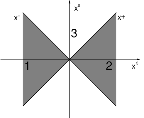
Fig. 1: Regions with different structures of the gauge potential:
In regions 1 and 2 we have the well known one nucleus solutions $\alpha_{1,2}$. While the gauge potential in the backward light cone is vanishing we have a nontrivial solution in the forward lightcone, region 3

In the abelian case even there the solutions would be directly given in terms of the single nucleus solutions as a sum of two pure gauge fields which again constitutes a pure gauge field. Hence in this case there would be no nontrivial effects on the classical field level. To generate photons and field strength one would have to resort to quantum effects. This is fundamentally different in the non-Abelian case. Obviously now, the sum of two pure gauge field is no longer a pure gauge field due to nonlinear effects, and therefore it does not solve the Yang Mills equations for the two nuclei problem. Nevertheless the one nucleus solutions provide initial conditions for the evolution of the gauge field in the forward light cone as discussed in [2].

In the remainder of this paper we will adopt the gauge condition

$$x^{+}A^{-}+x^{-}A^{+}=0$$ (8)

In this gauge the fields in the forward light cone can be cast in the form

$$A^{\pm} = \pm x^{\pm}\alpha(\tau,x_{\perp})$$

$$A^{i} = \alpha_{\perp}^{i}(\tau,x_{\perp})$$ (9)

where $\tau=\sqrt{2x^{+}x^{-}}$ is the proper time. Note that this representation does not introduce any physical assumption not already present in the single nucleus solution. The relation between $A^{\pm}$ is a consequence of the gauge condition. Further, the fact that the functions $\alpha(\tau,x_{\perp})$ and $\alpha_{\perp}^{i}(\tau,x_{\perp})$ do not depend on the space time rapidity $\eta=1/2\ln{x^{+}/x^{-}}$ is a natural consequence of the absence of a longitudinal length scale in our initial conditions with its infinitely thin nuclei moving at the speed of light.

Since the valence color charge densities vanish inside the light cone, the fields $A_{\mu}$ of eq. (9) should solve the homogeneous equations

$$\left[D_{\mu},F^{\mu\nu}\right] = 0$$ (10)

The initial conditions are determined by patching the solutions in the three regions (see Fig. 1) together and eliminating the discontinuities at $\tau=0$. This specifies the forward light cone fields $\left.\alpha^{i}_{\perp}\right|_{\tau=0}$ and $\left.\alpha\right|_{\tau=0}$ in terms of the known single nucleus solutions outside the forward light cone.

2 Perturbation theory

Using the form (9) of the gauge potential, the Yang-Mills equations (10) in the forward light cone are

$${1\over\tau^{3}}\partial_{\tau}\tau^{3}\partial_{\tau}\alpha+\left[D_{i},\left[D^{i},\alpha\right]\right] = 0$$

$${1\over\tau}\left[D_{i},\partial_{\tau}\alpha_{\perp}^{i}\right]+ig\tau\left[\alpha,\partial_{\tau}\alpha\right] = 0$$

$${1\over\tau}\partial_{\tau}\tau\partial_{\tau}\alpha^{i}_{\perp}-ig\tau^{2}\left[\alpha,\left[D^{i},\alpha\right]\right]-\left[D^{j},F^{ji}\right] = 0$$ (11)

Matching conditions on the solution lead to the initial conditions for $\alpha(\tau,x_{\perp})$ and $\alpha_{\perp}^{i}(\tau,x_{\perp})$ in terms of the single nucleus solutions $\alpha_{m}^{i}$:

$$\left.\alpha^{i}_{\perp}\right|_{\tau=0} = \alpha_{1}^{i}+\alpha_{2}^{i}$$

$$\left.\alpha\right|_{\tau=0} = {ig\over 2}\left[\alpha_{1}^{i},\alpha_{2}^{i}\right]$$ (12)

In this paper we construct solutions in the weak field limit by expanding first the initial conditions and then the fields within the forward light cone in powers of $\rho$.

Let us first concentrate on the initial conditions. To determine the initial conditions perturbatively, we need the single nucleus fields $\alpha_{m}^{i}$, $i=1,2$ to the appropriate order.

Recall that for a single nucleus, the Yang-Mills equations reduce to the two equations (7). The first states that $\alpha_{m}^{i}$ is a pure gauge field. The second equation determines $\alpha^{i}_{m}$ in terms of the charge density $\rho_{m}(x_{\perp})$ of the individual nuclei via

$$\partial^{i}\alpha_{m}^{i}\ \ =\ \ \partial^{i}\left\{-{1\over ig}U_{m}(x_{\perp})\partial^{i}U_{m}^{-1}\right\} = g\rho_{m}(x_{\perp})$$ (13)

To second order in $\rho$, the solution of (13) is

$${\alpha}_{m}^{i} = -\,\partial^{i}\phi_{m}+{ig\over 2}\left(\delta^{ij}-\partial^{i}{1\over{\nabla_{\!\!\perp}}^{2}}\partial^{j}\right)\left\{\left[\phi_{m},\partial^{j}\phi_{m}\right]+{\rm O}(\rho_{m}^{3})\right\}$$ (14)

where we have defined

$$\phi_{m} = -{g\over{\nabla_{\!\!\perp}}^{2}}\rho_{m}$$ (15)

Note that the first order term in (14) is longitudinal, whereas all higher corrections are transverse. Their sole purpose is to render $\alpha^{i}_{m}$ a pure gauge field. Plugging (14) into (12) gives us initial conditions up to second order in $\rho_{m}$.

To solve the equations of motion (11) in the forward light cone perturbatively, we also have to expand the gauge fields there in powers of $\rho_{m}$

$$\alpha = \sum\limits_{n=0}^{\infty}\alpha_{(n)}$$

$$\alpha^{i}_{\perp} = \sum\limits_{n=0}^{\infty}{\alpha^{i}_{\perp}}_{(n)}$$ (16)

First order:

To first order the equations of motion are necessarily linear

$${1\over\tau^{3}}\partial_{\tau}\tau^{3}\partial_{\tau}\alpha_{(1)}-{\nabla_{\!\!\perp}}^{2}\alpha_{(1)} = 0$$

$$\partial^{i}\partial_{\tau}{\alpha_{\perp}}_{(1)}^{i} = 0$$

$${1\over\tau}\partial_{\tau}\tau\partial_{\tau}{\alpha_{\perp}}_{(1)}^{i}-\left({\nabla_{\!\!\perp}}^{2}\delta^{ij}-\partial^{i}\partial^{j}\right){\alpha_{\perp}}_{(1)}^{j} = 0$$ (17)

They are to be solved subject to the initial conditions

$$\left.{\alpha}_{(1)}(\tau,x_{\perp})\right.|_{\tau=0} = 0$$

$$\left.{\alpha_{\perp}^{i}}_{(1)}(\tau,x_{\perp})\right.|_{\tau=0} = -\,\partial^{i}\left({\phi^{1}}+{\phi^{2}}\right)(x_{\perp})$$ (18)

The initial condition for the “$\pm$”-components to this order is trivial.

With these initial conditions, the first order solutions are completely specified and essentially trivial. We obtain vanishing $\alpha_{(1)}$

$$\alpha_{(1)}(\tau,x_{\perp}) = 0$$ (19)

and $\tau$-independent ${\alpha_{\perp}^{i}}_{(1)}$

$${\alpha_{\perp}^{i}}_{(1)}(\tau,x_{\perp}) = -\,\partial^{i}\left({\phi^{1}}+{\phi^{2}}\right)(x_{\perp})$$ (20)

which obviously is pure gauge.

To this order the problem is structurally identical to its abelian counterpart. Commutators do not appear neither in the equations of motion nor in the initial conditions (these contributions are necessarily at least second order in $\rho_{m}$), and hence no field strength is generated in the forward light cone.

Second order:

In the second order this changes immediately. Using the first order information almost all nonlinear terms drop from the second order equations which now read

$${1\over\tau^{3}}\partial_{\tau}\tau^{3}\partial_{\tau}\alpha_{(2)}-{\nabla_{\!\!\perp}}^{2}\alpha_{(2)} = 0$$

$$\partial^{i}\partial_{\tau}{\alpha_{\perp}}_{(2)}^{i} = 0$$

$${1\over\tau}\partial_{\tau}\tau\partial_{\tau}{\alpha_{\perp}}_{(2)}^{i}-\left({\nabla_{\!\!\perp}}^{2}\delta^{ij}-\partial^{i}\partial^{j}\right){\alpha_{\perp}}_{(2)}^{j}+ig\,\partial^{j}[{\alpha_{\perp}}_{(1)}^{j},{\alpha_{\perp}}_{(1)}^{i}] = 0$$ (21)

The only inhomogeneity in these equations comes from the – pure gauge – ${\alpha_{\perp}}^{i}_{(1)}$. In fact using the residual ($\tau$-independent) gauge freedom, we can remove the inhomogeneous piece altogether.

We define $\epsilon_{\mu}$ by

$$A_{\mu} = V(x_{\perp})\left[\epsilon_{\mu}-{1\over ig}\partial_{\mu}\right]V^{-1}(x_{\perp})$$ (22)

where $V(x_{\perp})=\exp-ig\phi_{\perp}(x_{\perp})$. $\phi_{\perp}(x_{\perp})$ is to be determined such that it removes nonlinear terms from the equations of motion for $\epsilon$ at least to second order. In fact, it turns out, that it is possible to remove the inhomogeneous terms up to third order in $\rho$ requiring

$$\partial^{i}\left.{\epsilon^{i}}\right.|_{\tau=0} = 0$$ (23)

In higher orders it is no longer possible to linearize the equations. Using equations (22) and (23) we find for ${\phi_{\perp}}$

$${\phi_{\perp}}=\phi_{1}+\phi_{2}+{\rm O}(\rho^{2})$$ (24)

With this choice of $V$ the first order solution vanishes

$$\epsilon_{(1)} \equiv 0$$

$$\epsilon^{i}_{(1)} \equiv 0$$ (25)

The second order equations become

$${1\over\tau^{3}}\partial_{\tau}\tau^{3}\partial_{\tau}\epsilon_{(2)}-{\nabla_{\!\!\perp}}^{2}\epsilon_{(2)} = 0$$

$$\partial^{i}\partial_{\tau}{\epsilon}_{(2)}^{i} = 0$$

$${1\over\tau}\partial_{\tau}\tau\partial_{\tau}{\epsilon}_{(2)}^{i}-\left(\delta^{ij}{\nabla_{\!\!\perp}}^{2}-\partial^{i}\partial^{j}\right){\epsilon}_{(2)}^{j} = 0$$ (26)

The initial conditions on $\alpha_{\perp}^{i}$ and $\alpha$ are transformed into

$$\left.\epsilon^{i}_{(2)}\right.|_{\tau=0} = -ig\ \left(\delta^{ij}-\partial^{i}{1\over{\nabla_{\!\!\perp}}^{2}}\partial^{j}\right)\left[\phi_{1},\partial^{j}\phi_{2}\right]$$ (27)

$$\left.\epsilon_{(2)}\right.|_{\tau=0} = {ig\over 2}\left[\partial^{i}{\phi_{1}},\partial^{i}{\phi_{2}}\right]$$ (28)

Obviously, the gauge condition $\partial^{i}\left.{\epsilon^{i}}\right.|_{\tau=0}=0$ in this order is preserved for all proper times $\tau$. Hence the “$i$”-components of the gauge field may be represented as

$$\epsilon^{i} = \epsilon^{ij}\partial^{j}\chi$$ (29)

Using $\epsilon$ and $\chi$, the second order Yang-Mills equations and initial conditions simplify even further. In terms of these variables, we finally obtain

$${1\over\tau^{3}}\partial_{\tau}\tau^{3}\partial_{\tau}\epsilon_{(2)}-{\nabla_{\!\!\perp}}^{2}\epsilon_{(2)} = 0$$

$${1\over\tau}\partial_{\tau}\tau\partial_{\tau}{\chi}_{(2)}-{\nabla_{\!\!\perp}}^{2}{\chi}_{(2)} = 0$$ (30)

and

$$\left.\epsilon_{(2)}\right.|_{\tau=0} = {ig\over 2}\left[\partial^{i}{\phi_{1}},\partial^{i}{\phi_{2}}\right]$$

$$\left.\chi_{(2)}\right.|_{\tau=0} = -ig\ \epsilon^{ij}\ \left[\partial^{i}{\phi_{1}},\partial^{j}{\phi_{2}}\right]$$ (31)

We stress that, even though the equations of motion (30) linearize to this order due to our gauge choice, the intrinsic nonlinearities of the system are very important. They show up in the initial conditions (31) which carry nontrivial physical information.

3 Perturbative solutions

To solve (30), we note that the equations are of form

$${1\over\tau^{m}}\partial_{\tau}\tau^{m}\partial_{\tau}f(\tau,x_{\perp})-{\nabla_{\!\!\perp}}^{2}f(\tau,x_{\perp})$$ (32)

where in our case $m=1,3$, $f=\chi,\epsilon$. Factorizing $\tau$ and $x_{\perp}$-dependence, we immediately identify the eigenfunctions

$$f_{k_{\perp}}(\tau,x_{\perp}) = (\omega_{k}\tau)^{1-m\over 2}\ Z_{\pm\left|{m-1\over 2}\right|}(\omega_{k}\tau)\ e^{ik_{\perp}^{j}x_{\perp}^{j}}$$ (33)

where $\omega_{k}=\sqrt{k_{\perp}^{2}}$ and $Z_{\nu}$ may in general be any linear combination of the Bessel functions $J_{\nu},N_{\nu}$.

The initial conditions (31) force our solutions to be regular at $\tau=0$ and thus preclude any admixture of Neumann-functions $N_{\nu}$.

A general solution is therefore of the form

$$F_{m}(\tau,x_{\perp}) = \int\!\!{d^{2}\!k_{\perp}\over(2\pi)^{2}}\ h_{m}(k_{\perp})\ f_{k_{\perp}}(\tau,x_{\perp})$$ (34)

$$= \int\!\!{d^{2}\!k_{\perp}d^{2}\!y_{\perp}\over(2\pi)^{2}}\ e^{ik_{\perp}^{j}(x_{\perp}-y_{\perp})^{j}}\ h_{m}(y_{\perp})\ (\omega_{k}\tau)^{1-m\over 2}\ J_{\left|{m-1\over 2}\right|}(\omega\tau)$$

For equations (30) this yields

$$\epsilon_{(2)}(\tau,x_{\perp}) = \int\!\!{d^{2}\!k_{\perp}d^{2}\!y_{\perp}\over(2\pi)^{2}}e^{ik_{\perp}^{j}(x-y)_{\perp}^{j}}\ h_{3}(y_{\perp})\ {1\over\omega\tau}J_{1}(\omega\tau)$$

$$\chi_{(2)}(\tau,x_{\perp}) = \int\!\!{d^{2}\!k_{\perp}d^{2}\!y_{\perp}\over(2\pi)^{2}}\ e^{ik_{\perp}^{j}(x-y)_{\perp}^{j}}\ h_{1}(y_{\perp})J_{0}(\omega\tau)$$ (35)

with $h_{3}$ and $h_{1}$ determined by the initial conditions eq.(31) as

$$h_{3}(x_{\perp}) = {ig}\left[\partial^{i}\phi_{1},\partial^{i}\phi_{2}\right](x_{\perp})$$

$$h_{1}(x_{\perp}) = -ig{\epsilon^{ij}\over{\nabla_{\!\!\perp}}^{2}}\left[\partial^{i}\phi_{1},\partial^{j}\phi_{2}\right](x_{\perp})$$ (36)

In the following we will need the large $\tau$ asymptotics of the solutions:

$$\chi_{(2)}(\tau,x_{\perp}) = \int\!\!{d^{2}\!k_{\perp}\perp\over(2\pi)^{2}}\ e^{ik_{\perp}^{j}x_{\perp}^{j}}\ h_{1}(k_{\perp})\ \left\{{\sqrt{2/\pi}\over(\omega\tau)^{1/2}}\cos(\omega\tau-{\pi\over 4})+{\rm O}({1\over\tau^{3/2}})\right\}$$ (37)

$$\epsilon_{(2)}(\tau,x_{\perp}) = \int\!\!{d^{2}\!k_{\perp}\over(2\pi)^{2}}e^{ik_{\perp}^{j}x_{\perp}^{j}}\ h_{3}(k_{\perp})\ \left\{{\sqrt{2/\pi}\over(\omega\tau)^{3/2}}\cos(\omega\tau-{3\over 4}\pi)+{\rm O}({1\over\tau^{3/2}})\right\}$$ (38)

4 Distribution functions

The solutions of the Yang Mills equations at asymptotically large $\tau$ are of the form

$$\epsilon^{a}(\tau,x_{\perp}) = \int{{d^{2}k_{\perp}}\over{(2\pi)^{2}}}{1\over\sqrt{2\omega}}\left\{a_{1}^{a}(\vec{k}_{\perp}){1\over\tau^{3/2}}e^{ik_{\perp}\cdot x_{\perp}-i\omega\tau}+C.C.\right\}$$

$${\epsilon}^{a,i}(\tau,x_{\perp}) = \int{{d^{2}k_{\perp}}\over{(2\pi)^{2}}}\kappa^{i}{1\over\sqrt{2\omega}}\left\{a_{2}^{a}(k_{\perp}){1\over\tau^{1/2}}e^{ik_{\perp}x_{\perp}-i\omega\tau}+C.C.\right\}$$ (39)

Here $\omega=\mid k_{\perp}\mid$, and $\kappa^{i}=\epsilon^{ij}k^{j}/\omega$. The notation $C.C.$ means complex conjugate.

To derive an expression for the energy density, we recall that $\tau$ is large. Near $z=0$, this implies that in the range of $z$ where $\tau\sim t\gg z$ the solutions are $z$ independent. This means they asymptotically have zero $p_{z}$. Now suppose we are at any value of $z$, and $\tau$ is large but $t\sim z$. We can do a longitudinal boost to $z=0$ without changing the solution. Again in this frame the solution has zero $p_{z}$. We see therefore that for the asymptotic solutions the space time rapidity is one to one correlated with the momentum space rapidity, that is at asymptotic times we find that

$$\eta={1\over 2}\ln(x^{+}/x^{-})=y={1\over 2}\ln(p^{+}/p^{-})$$ (40)

To proceed further, we compute the energy density in the neighborhood of $z=0$. Here asymptotically $\tau=t$. The energy in a box of size $R$ in the transverse direction and $dz$ in the longitudinal direction, with $L\ll t$ becomes [6]

$$dE={{dz}\over t}\int{{d^{2}k_{\perp}}\over{(2\pi)^{2}}}\omega\sum_{i,b}\mid a_{i}^{b}(k_{\perp})\mid^{2}$$ (41)

Recalling that $dy=dz/t$, we find that

$${{dE}\over{dyd^{2}k_{\perp}}}={1\over{(2\pi)^{3}}}\omega\sum_{i,b}\mid a_{i}^{b}(k_{\perp})\mid^{2}$$ (42)

and the multiplicity distribution of gluons is

$${{dN}\over{dyd^{2}k_{\perp}}} = {1\over\omega}{{dE}\over{dyd^{2}k_{\perp}}}$$ (43)

As we expect for a boost covariant solution, the multiplicity distribution is rapidity invariant.

This is now easily compared to the asymptotic behavior of the second order solutions (38), (37). We read off that

$$a_{1}(k_{\perp}) = {1\over\sqrt{\pi}}{h_{3}(k_{\perp})\over\omega}$$

$$a_{2}(k_{\perp}) = {1\over\sqrt{\pi}}i\omega h_{1}(k_{\perp})$$ (44)

Hence we get the distribution function

$${{dN}\over{dyd^{2}k_{\perp}}} = {1\over\omega}{{dE}\over{dyd^{2}k_{\perp}}}$$ (45)

$$= {1\over{(2\pi)^{3}}}\sum_{i}2\ {\rm tr}\ a_{i}(k_{\perp})a_{i}^{\dagger}$$

$$= {1\over{(2\pi)^{3}}}\sum_{i}{2\over\pi}\ {\rm tr}\left\{{h_{3}(k_{\perp})h_{3}^{\dagger}(k_{\perp})\over\omega^{2}}+\omega^{2}h_{1}(k_{\perp})h_{1}^{\dagger}(k_{\perp})\right\}$$

Now we use that

$$h_{3}(k_{\perp}) = \int\!\!d^{2}\!y_{\perp}e^{-ik_{\perp}{\cdot}y_{\perp}}\ ig\left\{\left[\partial^{i}\phi_{1},\partial^{i}\phi_{2}\right]\right\}(y_{\perp})$$

$$h_{1}(k_{\perp}) = \int\!\!d^{2}\!y_{\perp}e^{-ik_{\perp}{\cdot}y_{\perp}}\ \left\{-ig{\epsilon^{ij}\over{\nabla_{\!\!\perp}}^{2}}\left[\partial^{i}\phi_{1},\partial^{j}\phi_{2}\right]\right\}(y_{\perp})$$ (46)

$$= {1\over\omega^{2}}\int\!\!d^{2}\!y_{\perp}e^{-ik_{\perp}{\cdot}y_{\perp}}\ \left\{ig\epsilon^{ij}\left[\partial^{i}\phi_{1},\partial^{j}\phi_{2}\right]\right\}(y_{\perp})$$

and get

$${{dN}\over{dyd^{2}k_{\perp}}} = {\rm S}_{\perp}{g^{2}\over{(2\pi)^{3}}}{2\over\pi k_{\perp}^{2}}\left[\delta^{ij}\delta^{kl}+\epsilon^{ij}\epsilon^{kl}\right]\int\!\!d^{2}\!x_{\perp}e^{ik_{\perp}{\cdot}x_{\perp}}$$ (47)

$$\quad{\rm tr}\left\langle\left[\partial^{i}\phi_{1},\partial^{j}\phi_{2}\right](x_{\perp})\left[\partial^{k}\phi_{1},\partial^{l}\phi_{2}\right]^{\dagger}(0)\right\rangle_{\rho}$$

where, S_⟂ is the transverse area of the system. As indicated, we have to average over $\rho$ with the Gaussian weight eq.( (5)). Using (15) we find

$$\langle\phi_{m}^{a}(x_{\perp})\phi_{n}^{b}(y_{\perp})\rangle_{\rho} = g^{2}\,\mu^{2}\ \delta^{mn}\ \delta^{ab}\ \int\!\!{d^{2}\!p_{\perp}\over(2\pi)^{2}}{e^{ip_{\perp}{\cdot}(x-y)_{\perp}}\over p_{\perp}^{4}}$$ (48)

and the above turns into

$${{dN}\over{dyd^{2}k_{\perp}}} = {\rm S}_{\perp}{g^{6}\over{(2\pi)^{3}}}{2\over\pi k_{\perp}^{2}}\left[\delta^{ij}\delta^{kl}+\epsilon^{ij}\epsilon^{kl}\right]$$ (49)

$$\mu^{4}{\rm tr}\left([\tau^{a},\tau^{b}][\tau^{b},\tau^{a}]\right)\int\!\!{d^{2}\!p_{\perp}\over(2\pi)^{2}}{p^{i}p^{k}(p+k)^{j}(p+k)^{l}\over p^{4}(p+k)^{4}}$$

$$= {\rm S}_{\perp}{g^{6}\over{(2\pi)^{3}}}{2\over\pi k_{\perp}^{2}}\mu^{4}N_{c}(N_{c}^{2}-1)\int\!\!{d^{2}\!p_{\perp}\over(2\pi)^{2}}{1\over p^{2}(p+k)^{2}}$$

The integral in equation (49) is infrared divergent. This however is an artifact of the weak field expansion employed above. As discussed in [1, 4, 5, 2], the inclusion of higher order terms for the initial fields would generate a mass scale of order $\alpha_{s}\mu$ and hence regulate this divergence. With logarithmic accuracy we obtain therefore

$${{dN}\over{dyd^{2}k_{\perp}}} = {\rm S}_{\perp}{g^{6}\over{(2\pi)^{3}}}{2\over\pi}\mu^{4}N_{c}(N_{c}^{2}-1)\ \ {1\over 2\pi}{1\over k_{\perp}^{4}}\ln{k_{\perp}^{2}\over(\alpha_{s}\mu)^{2}}$$ (50)

This is the main result of this work.

5 Conclusion

In this paper we have calculated the high $k_{\perp}$ asymptotics of the distribution function of gluons produced in a collision of two ultrarelativistic heavy nuclei in the framework of the McLerran-Venugopalan model.

Our result, eq. (50) has a very natural interpretation in analogy to the naive parton model. The number of produced gluons in the parton model is given by

$$N(k_{\perp})=\int d^{2}p_{\perp}N_{1}(p_{\perp})N_{2}(k_{\perp}-p_{\perp})\sigma(p_{\perp},k_{\perp})$$ (51)

where $N_{m}(q_{\perp})$ is the probability to find a gluon with transverse momentum $q_{\perp}$ in the $m$-th nucleus, and $\sigma$ is the cross section for production of the gluon with momentum $k_{\perp}$ in the final state in the collision of the two gluons. To the lowest order in perturbation theory the cross section is

$$\sigma(k_{\perp})\propto\frac{\alpha_{s}}{k_{\perp}^{2}}$$ (52)

The distribution functions for the one nucleus case $N_{m}$ were calculated in [1, 4] and were found to have the same functional form as in the lowest order in perturbation theory

$$N_{m}(q_{\perp})\propto\frac{\alpha_{s}\mu^{2}}{q_{\perp}^{2}}$$ (53)

Substituting this into eq.(51) gives the result of eq.(50).

Indeed the calculation performed in this paper can be represented in terms of Feynman diagrams. The gluon distribution function of eq.(50) has a representation of Fig. 2.

Fig. 2: Diagrammatic representation of the lowest order distribution function

The reader may have noticed one peculiarity in the preceding discussion. Although we have been using the parton model notations, some of the gluons involved in the process depicted on Fig. 2 are virtual. To produce the real final state gluon, the internal gluons must be off shell with virtuality of order of their momentum. In fact if one wants to think about this process in terms of real partons, it must be represented as “two quarks go into two quarks and a gluon”, rather than “two gluons go into one gluon”, which is kinematically forbidden for on shell particles.

As we have seen, to this order our calculation essentially reproduces perturbation theory. The reason is that we have expanded in powers of the valence charge density, and thereby have ignored the fact that the classical fields involved are expected to be strong. The real nonperturbative nature of this approach will become apparent when those are fully taken into account. Some of the qualitative consequences of such an analysis however, can be understood already at this point. Consider for example, the total multiplicity of produced gluons.

$$N=\int d^{2}k_{\perp}{{dN}\over{dyd^{2}k_{\perp}}}$$ (54)

Since ${{dN}\over{dyd^{2}k_{\perp}}}$ is proportional to the transverse area of the system, and is a function of the dimensionless ratio $\mu^{2}/k_{\perp}^{2}$, the integral has to be proportional to $S_{\perp}\mu^{2}$. Remembering that for large nuclei $\mu$ scales with the number of nucleon in the nucleus $A$ as $\mu^{2}\propto A^{1/3}$, we conclude that for large nuclei the total multiplicity scales as

$$N\propto A$$ (55)

On the other hand, the total multiplicity at momenta larger than some fixed momentum $p\gg\alpha\mu$ will coincides with the perturbative result

$$N=\int\limits_{k_{\perp}^{2}\geq p^{2}}d^{2}k_{\perp}{{dN}\over{dyd^{2}k_{\perp}}}\propto S_{\perp}\mu^{4}\propto A^{4/3}$$ (56)

Therefore it is very important to go beyond the weak field expansion and incorporate truly nonperturbative effects due to strong classical fields.

In comparing our results with the parton cascade model of Geiger et al [7, 8, 9] one should keep in mind the following differences between the two approaches. In the parton cascade, the leading order in $\alpha_{s}$ scattering occurs by gluon gluon scattering. This populates the high $p_{\perp}$ tail of the distribution by scatterings of low $p_{\perp}$ gluons. In our case, we have an intrinsic $p_{\perp}$ for the gluons and the gluons are far enough off mass shell so that we can produce high $p_{\perp}$ gluons by glue-glue goes to single gluon scattering. Consequently, although the $p_{\perp}$ dependence of the two results is similar, in the high $p_{\perp}$ region we have a different dependence on $\alpha_{S}$. We have one power less, since the factor $\alpha^{2}\mu^{2}$ in eq. (50) just sets the scale of the intrinsic single nucleus glue distribution.

The scattering processes, which are leading in our approximation are also present in cascade codes as composite processes $qq\rightarrow qqg$, where some of the quarks are off shell by an amount $p_{\perp}^{2}$. Although these contributions are formally of order $\alpha^{3}$, for very large nuclei the quark distribution functions will be large and these processes may become leading. This seems to be the natural point of contact between the two approaches.

Of course at some $p_{\perp}\gg\mu$, our approximations for computing the gluon distribution function break down. This presumably first occurs when gluon bremsstrahlung softens the high $p_{\perp}$ distribution from its $1/p_{\perp}^{2}$ behavior, and the spectrum steepens. The main point is however not what happens in the tail of the distribution. This is simply where it is most easy to compute. In the center of the $p_{\perp}$ distribution of produced gluons, the gluons arise from a non-linear evolution of the gluons fields. This is cause by the quantum mechanical nature of the initial state and the charge coherence of the initial state interactions. In this case, the final state distribution of gluons bears scant resemblance to that of the initial distribution convoluted over hard gluon scattering. Before one knows whether there are substantial quantitative differences, one must of course numerically solve the problem for gluons in the center of the distribution.

References

• [1] L. McLerran and R. Venugopalan. Phys. Rev., D49 (1994), 2233.
• [2] A. Kovner, L. McLerran, and H. Weigert. Gluon Production from Non-Abelian Weizsäcker-Williams Fields in Nucleus-Nucleus Collisions. submitted to Phys. Rev. D hep-ph/9502289, 1995.
• [3] A. Mueller. Nucl. Phys., B425 (1994), 373.
• [4] L. McLerran and R. Venugopalan. Phys. Rev., D49 (1994), 3352.
• [5] L. McLerran and R. Venugopalan. Phys. Rev., D50 (1994), 2225.
• [6] J. P. Blaizot and A. Mueller. Nucl. Phys., B289 (1987), 847.
• [7] K. Geiger and B. Müller. Nucl. Phys., B369 (1992), 600.
• [8] K. Geiger. Phys. Rev., D47 (1993), 133.
• [9] K. Geiger and B. Müller. Cern Preprint CERN-TH 7313/94, 1994.