Abstract

The Higgs couplings to matter fields are proportional to their masses. Thus Higgs amplitudes can be obtained by differentiating amplitudes without Higgs with respect to masses. We show how this well-known statement can be extended to higher order when renormalization effects are taken into account. We establish the connection with the Callan-Symanzik and renormalization group equations and consider also pseudoscalar Higgs couplings to fermions. Furthermore, we address the case where the Higgs couples to a heavy particle that is integrated out from the low-energy effective Lagrangian. We derive effective interactions where mass logarithms are resummed by renormalization-group methods, and give expansions of the results up to next-to-leading order.

1 Introduction

The Higgs boson provides a simple mechanism to accommodate massive vector bosons and fermions in the standard model. Present-day experiments, together with calculations of Higgs interactions up to two-loop order in some cases, have been used to establish lower limits for Higgs masses approaching the $W$ and $Z$ mass range, and the next generation of colliders may give a definite answer to the question of its existence.

A widely used tool in the study of Higgs interactions are low-energy theorems (soft-Higgs theorems), which play a role comparable to the low-energy theorems for pion amplitudes in hadronic physics. They rely on the fact that the explicit breaking of scale invariance by the Higgs interactions can be employed to relate tree-level amplitudes with different numbers of zero-momentum Higgs fields [1]. This theorem has been extended to one-loop amplitudes, where scale invariance becomes anomalously broken, and it has been observed that there exists some connection with the scaling functions (beta functions) of renormalization group theory [2]. Various applications can be found in the literature [3, 4], and recently with its help two-loop amplitudes were calculated in the heavy-top limit [5, 6, 7, 8], where algorithms were devised to take into account the renormalization effects. However, the role of scale anomalies in higher order has remained unclear in the present context [9], and thus the precise form of the theorem for renormalized amplitudes in the general case has remained unknown. The purpose of the present paper is to clarify this issue and to provide a general survey of soft-Higgs theorems in the framework of renormalized perturbation theory.

Since it is conceptually simpler, we shall discuss first the soft-Higgs theorem for pseudoscalar Higgs bosons, which exist in models with an extended Higgs sector. In that case the relevant symmetry is chiral invariance [10], anomalously broken by the well-known triangle anomaly [11]. Next, the theorem for scalar bosons will be developed, where the anomalies proliferate. We shall show how they are controlled by the Callan-Symanzik equation, and give the explicit form of the theorem both in on-shell and minimal subtraction (MS or $\overline{\rm MS}$) schemes. The latter allows for the introduction of effective-theory methods, which already have been applied in [5]. That the effective-theory picture is appropriate, follows from the observation that the Higgs coupling to the heaviest particle (e.g., the top quark) is dominant, and since the soft-Higgs theorem applies at low energies (and small Higgs masses), such a particle should be integrated out from the low-energy theory. Furthermore, when this method is used, logarithms of large mass ratios are easily summed by the renormalization group. We shall derive the form of the soft-Higgs theorem in the effective theory and show that this framework provides a natural description of all coefficients in terms of scaling functions, which we shall give in some detail. In an appendix we give the formulas in a form which is directly applicable in a next-to-leading order calculation, and demonstrate their use in a sample calculation that can be compared to the calculational methods used in the literature.

2 Pseudoscalars and chiral symmetry

Before we consider the scalar Higgs, let us investigate the couplings of a pseudoscalar (CP-odd) Higgs boson, predicted, e.g., by supersymmetric extensions of the standard model, to fermions. To keep things simple, we allow only one external pseudoscalar in the amplitude.

We apply an infinitesimal global chiral transformation

$$\delta\psi=-i\epsilon g_{A}\gamma_{5}\psi/2,$$ (1)

where $g_{A}$ is the coupling of the fermion $\psi$ to the pseudoscalar Higgs $A$:

$${\cal L}_{A}=g_{A}\bar{\psi}i\gamma_{5}A\psi,$$ (2)

The variation of the fermion mass term introduces an additional term in the Lagrangian

$$\delta{\cal L}=\epsilon g_{A}m\bar{\psi}i\gamma_{5}\psi,$$ (3)

which may be interpreted as an imaginary contribution to the masses of left- and right-handed fermions [10]. To first order in $\epsilon$, the fermion propagator is modified into

$$G_{\epsilon}(k)=i\frac{k\hskip-5.0pt/+m+i\epsilon g_{A}m\gamma_{5}}{k^{2}-m^{2}}.$$ (4)

Thus we have the relation

$$\frac{\partial}{\partial\epsilon}{\cal L}=m\frac{\delta{\cal L}_{A}}{\delta A}=\delta{\cal L}.$$ (5)

In addition to (3), the variation (1) introduces terms mixing the scalar ($H$) and pseudoscalar ($A$) couplings to fermions, since these interactions also break chiral invariance. This mixing can be compensated by a redefinition of the $H$ and $A$ fields (in the light-Higgs limit) and will not be considered here.

Apart from its coupling to fermions, the $A$ field can couple to other Higgs or Goldstone fields. The corresponding interaction operator will be called ${\cal A}$. This term is not obtained by the differentiation with respect to $\epsilon$:

$$\delta{\cal L}=m\frac{\delta{\cal L}}{\delta A}-{\cal A}.$$ (6)

For the full amplitude, differentiation with respect to $\epsilon$ obviously will give no diagrams with ${\cal A}$ insertions. These have to be calculated separately, but in the limit of light $A$ they can be neglected, since the Higgs masses are proportional to self-couplings.

The relation (6) may be extended to a relation for $\Gamma$, the generating functional of one-particle irreducible (1PI) vertices, which is in tree approximation equal to the action $\int{\cal L}$. First we write down the identity describing the irreducible interactions of one zero-momentum $A$ in terms of zero-momentum operator insertions:

$$m\int\frac{\delta}{\delta A}\Gamma^{(0)}|_{H=A=0}=\int\delta{\cal L}\Downarrow\Gamma^{(0)}|_{H=A=0}+\int{\cal A}\Downarrow\Gamma^{(0)}|_{H=A=0}.$$ (7)

(We use ${\cal A}\Downarrow\Gamma$ as a shorthand for the 1PI generating functional with an insertion of the renormalized operator ${\cal A}$.) It holds in the presence of quantum effects, up to scheme-dependent universal corrections (denoted by $\alpha_{A}$) referring to the particular renormalization conditions imposed on the $A$ field (cf. Sec. 3):

$$m(1+\alpha_{A})\int\frac{\delta}{\delta A}\Gamma|_{H=A=0}=\int\delta{\cal L}\Downarrow\Gamma|_{H=A=0}+\int{\cal A}\Downarrow\Gamma|_{H=A=0}.$$ (8)

This is seen by investigating the diagrams contributing to both sides.

The nontrivial part is the quantum extension of the Ward identity (5) of chiral symmetry. However, the answer is well known [11]:

$$\frac{\partial}{\partial\epsilon}\Gamma(\epsilon)|_{\epsilon=0}=\int\delta{\cal L}\Downarrow\Gamma-sg_{A}\int{\rm tr}\left[F\tilde{F}\right]\Downarrow\Gamma.$$ (9)

where $s$ is a constant equal to its one-loop value, and $F$ ($\tilde{F}$) denotes the (dual) field strength tensor. Thus we obtain

$$m(1+\alpha_{A})\int\frac{\delta}{\delta A}\Gamma=\frac{\partial}{\partial\epsilon}\Gamma+sg_{A}\int{\rm tr}\left[F\tilde{F}\right]\Downarrow\Gamma+\int{\cal A}\Downarrow\Gamma,$$ (10)

where $\epsilon$, $H$, and $A$ have to be set to zero after differentiation.

The relation (10) is readily verified in an explicit calculation. If the integrand contains an open fermion line, the insertion of a zero-momentum $A$ gives the expression

$$i\frac{k\hskip-5.0pt/+m}{k^{2}-m^{2}}i(g_{A}i\gamma_{5})i\frac{k\hskip-5.0pt/+m}{k^{2}-m^{2}}=i\frac{ig_{A}\gamma_{5}}{k^{2}-m^{2}}=\frac{1}{m}\frac{\partial}{\partial\epsilon}G_{\epsilon}(k)|_{\epsilon=0},$$ (11)

where we have used the anticommuting nature of $\gamma_{5}$. Thus the theorem is trivially satisfied. In fermion loops, the behavior of $\gamma_{5}$ is accounted for by the triangle anomaly term in (10).

Since we work only to first order in $\epsilon$, it appears only in the numerator and the differentiation does not affect the large-momentum behavior. Thus there is no room for renormalization to introduce further anomalies. If we were to derive the interaction of several pseudoscalar particles, apart from other complications the quadratic term in $\epsilon$ would give a mass shift, so that renormalization effects came into play. Then the scale anomalies introduced in the next section would have also to be considered. They are CP-even and therefore do not occur in the first-order $A$ couplings.

As mentioned in the introduction, the theorem (10) is valid for vanishing four-momentum $p_{A}$. Only when the mass $m_{A}$ can be neglected compared to $m$ — in which case also the contribution of ${\cal A}$ will be small — this approaches the amplitude for an on-shell $A$ particle with $\vec{p}_{A}=0$. For this reason, (10) may be called a soft-$A$ theorem (for applications, see ref. [8], and references cited therein).

3 Scalars and scale transformations

Turning over to scalar Higgs couplings in a theory such as the Standard Model, we divide the Lagrangian into three parts

$${\cal L}={\cal L}_{0}+{\cal L}_{GF}+{\cal L}_{H},$$ (12)

where the first term denotes the Lagrangian of gauge boson and matter fields, including interactions with the Higgs fields, the second part is the gauge-fixing and ghost part of the Lagrangian, and the last term contains the pure Higgs Lagrangian, i.e., the self-interactions of the physical Higgs $H$ and the Goldstone fields.

We assume that mass terms in ${\cal L}_{0}$ are generated only through the Higgs vacuum expectation value $v$, so that

$${\cal L}_{0}(m_{i},H)={\cal L}_{0}(m_{i}+g_{i}H)$$ (13)

where the mass $m_{i}$ is given by

$$m_{i}=g_{i}v.$$ (14)

Similar to the connection between pseudoscalar couplings and chiral transformations described in the preceding section, scalar Higgs couplings are related to scale transformations. These act on the fields as

$$\delta\psi=(d_{\psi}+x\cdot\partial)\psi,$$ (15)

where $d_{\psi}$ is the canonical dimension of the generic field $\psi$. With $d_{\psi}=3/2$ for fermions and $d_{\psi}=1$ for bosons, the variation of the action reads

$$\int\delta{\cal L}=\int\left(v\frac{\partial{\cal L}_{0}}{\partial v}+\delta{\cal L}_{GF}+\delta{\cal L}_{H}\right),$$ (16)

since scale invariance is broken by a nonvanishing value of $v$, and by dimensionful parameters in the gauge-fixing and Higgs parts of the Lagrangian. Using (13), this can be rewritten as

$$\int\delta{\cal L}=\int\left(v\frac{\delta{\cal L}}{\delta H}-v\frac{\delta{\cal L}_{H}}{\delta H}+\delta{\cal L}_{GF}+\delta{\cal L}_{H}\right)$$ (17)

or

$$\int\delta{\cal L}=v\int\frac{\delta{\cal L}}{\delta H}-\int{\cal H}.$$ (18)

Similar to the operator ${\cal A}$ in the preceding section, the operator ${\cal H}$ summarizes Higgs self-couplings and couplings to gauge fields generated by the gauge fixing. The diagrams with ${\cal H}$ insertions have to be calculated explicitly. When they contain Higgs (Goldstone) self-couplings, in the light-Higgs limit they can be neglected compared to diagrams with couplings to heavy particles. However, the mass parameter in the gauge-fixing part (in a ’tHooft gauge, for instance) introduces a spurious variation $\delta{\cal L}_{GF}$ that is not related to a Higgs coupling. In one-loop order it can be separated just by omitting the derivative with respect to this gauge-fixing mass in the relations below, but from the two-loop order on it becomes entangled into the renormalization procedure. There are several possibilities to deal with this complication: one could either use the background-field method employed in [12], which requires the calculation of more diagrams, or impose the additional restriction that also the gauge boson masses have to be neglected, or turn over to a mass-independent renormalization scheme. The latter will be done in the next section.

The extension of (17) to irreducible vertices has the form

$$(1+\alpha_{H})v\int\frac{\delta}{\delta H}\Gamma=\int\delta{\cal L}\Downarrow\Gamma+\int{\cal H}\Downarrow\Gamma.$$ (19)

The unrenormalized diagrams which do not involve Higgs (Goldstone) self-couplings, contributing to the relation (19), are identical on both sides. The same is true for the counterterms, except for the renormalization of the external Higgs field: In the on-shell scheme the left-hand side is renormalized with the momentum $p_{H}$ flowing into the vertex satisfying $p_{H}^{2}=m_{H}^{2}$, whereas the right-hand side is defined for vanishing momentum $p_{H}$. Corrections proportial to $m_{H}^{2}$ are consistently absorbed into ${\cal H}$, so that there remains an overall multiplicative factor, denoted by $1+\alpha_{H}$. Any possible correction involving Higgs (Goldstone) self-couplings is also absorbed in ${\cal H}$.

We can employ the Ward identity of scale invariance to get rid of the operator $\delta{\cal L}$ in (19) and obtain in this way a nontrivial statement. Although scale invariance is broken by quantum corrections [13], the quantum action principles [14] tell us that all corrections (anomalies) are given by a linear combination of local operator insertions with the appropriate quantum numbers and dimension. The resulting anomalous Ward identity of scale transformations is known as the Callan-Symanzik equation [15]. For an abelian Higgs model a detailed derivation is given in [12]. Here we simply generalize the result for a general Higgs model in an on-shell scheme: The relation (19) can be replaced by

$$(1+\alpha_{H})v\int\frac{\delta}{\delta H}\Gamma^{(n_{1},\ldots)} = \left(\sum_{i}m_{i}\frac{\partial}{\partial m_{i}}+\beta_{i}\frac{\partial}{\partial g_{i}}+\frac{n_{i}}{2}\gamma_{i}+\delta_{i}\frac{\partial}{\partial\xi_{i}}\right)\Gamma^{(n_{1},\ldots)}$$ (20)

$$+\,\int{\cal H}\Downarrow\Gamma^{(n_{1},\ldots)}.$$

for an irreducible vertex with $n_{i}$ external fields of species $i$, which is given by

$$\Gamma^{(n_{1},\ldots)}=\frac{\delta^{n_{1}}}{\delta\psi_{1}^{n_{1}}}\cdots\Gamma.$$ (21)

The $\xi_{i}$ are gauge parameters, and ${\cal H}$ can be neglected, as discussed above.

The coefficients $\alpha$, $\beta$, $\gamma$, $\delta$ have to be determined order by order in perturbation theory. They are universal for all processes, but they are mass-dependent and are not simply related to the familiar scaling functions in a mass-independent scheme, which will be introduced in the next section. Some of them are determined by the symmetry. In particular, all but one of the coupling constants are usually expressed in terms of masses, so that their beta functions may be identified as mass beta functions [12], due to the normalization conditions one imposes.

Introducing the concept of bare parameters, which can also be used for a simple derivation of the Callan-Symanzik equation [13], the coefficients can be expressed as derivatives of the renormalized parameters with respect to bare masses. The relation (20) thus involves the operations carried out in [6, 7] in reverse order: If instead of renormalizing after taking the derivative with respect to bare masses, the renormalized amplitudes are differentiated, one has to correct for the derivatives of the renormalized parameters. These are the corrections summarized in (20).

4 Renormalization group

The relation (20) has been derived within the context of an on-shell scheme, where all dimensionful parameters are expressed in terms of the physical masses of the theory. When a minimal subtraction scheme (MS or $\overline{\rm MS}$) is used, the derivation is greatly simplified. The price are complicated, but calculable, relations of the parameters to physical observables.

Taken literally, a minimal subtraction scheme does not subtract the tadpole diagrams completely. This is a minor problem: In terms of irreducible diagrams, only the Higgs one-point function is affected, and since it is a constant, the finite part can completely be subtracted without affecting properties of the dimensional renormalization procedure that follow from mass independence: tadpoles are simply omitted.

To lowest order (tree level), the relation (20) reads

$$v\int\frac{\delta}{\delta H}\Gamma^{(n_{1},\ldots)}=\sum_{i}m_{i}\frac{\partial}{\partial m_{i}}\Gamma^{(n_{1},\ldots)}\\ +\int{\cal H}\Downarrow\Gamma^{(n_{1},\ldots)}.$$

Here we exclude the mass term in the gauge fixing from the derivative, so that ${\cal H}$ does not contain spurious couplings and is truly negligible in the light-Higgs limit.

In the dimensional renormalization scheme, the quantum action principles hold in the strong sense [16], so that (4) is valid without corrections even after renormalization, if the running parameters at the scale $\mu$ are inserted everywhere. Stated differently, the coefficients $\beta$ and $\gamma$ appearing in (20), which are related to mass derivatives of the renormalized parameters, vanish identically: the renormalization factors are mass-independent.

It is now easy to get rid of the mass derivatives in favor of familiar renormalization group coefficients, if we have a one-scale problem. The case of multiple scales will be considered in the next sction. We thus put all other masses and external momenta to zero, ignoring infrared divergences. (If some care in the renormalization of subdivergences is taken, they may be regulated dimensionally.) We use the MS or $\overline{\rm MS}$ scheme. Then any renormalized vertex function with mass dimension $d$ and $n_{\ell}$ external light fields of species $\ell$ can be expressed as

$$\Gamma(m(\mu),\mu)=m(\mu)^{d}\tilde{\Gamma}(\ln{\textstyle\frac{\mu}{m(\mu)}},g(\mu)),$$ (22)

with a dimensionless function $\tilde{\Gamma}$. Defining the mass anomalous dimension

$$\frac{d\ln m(\mu)}{d\ln\mu}=-\gamma_{m}(\mu),$$ (23)

we derive

$$\frac{d}{d\ln\mu}\Gamma(\mu)=\left(d-(1+\gamma_{m})\frac{\partial}{\partial\ln m(\mu)}+\beta_{i}\frac{\partial}{\partial g_{i}}\right)\Gamma(m(\mu),\mu).$$ (24)

On the other hand, the vertex function satisfies a renormalization group equation

$$\frac{d}{d\ln\mu}\Gamma(\mu)=-\frac{n_{\ell}}{2}\gamma_{\ell}\Gamma(\mu),$$ (25)

so that

$$\frac{\partial}{\partial\ln m(\mu)}\Gamma(m(\mu),\mu)=\frac{1}{1+\gamma_{m}}\left(\beta_{i}\frac{\partial}{\partial g_{i}}+d+\frac{n_{\ell}}{2}\gamma_{\ell}\right)\Gamma(m(\mu),\mu).$$ (26)

The definitions of the scaling coefficients are

$$\beta_{i} = \frac{d}{d\ln\mu}g_{i},$$ (27)

$$\gamma_{i} = \frac{d}{d\ln\mu}\ln Z_{i}.$$ (28)

Thus the soft-Higgs theorem in the dimensional renormalization scheme has the form

$$v\int\frac{\delta}{\delta H}\Gamma^{(n_{1},\ldots)} = \frac{1}{1+\gamma_{m}}\left(\beta_{i}\frac{\partial}{\partial g_{i}}+d+\frac{n_{i}}{2}\gamma_{i}\right)\Gamma^{(n_{1},\ldots)}$$ (29)

$$+\,\int{\cal H}\Downarrow\Gamma^{(n_{1},\ldots)}.$$

This looks very similar to (20), but without the derivative with respect to the mass: In this scheme the coupling of the Higgs is given by scaling coefficients only, for vanishing external momenta.

5 Heavy and light fields: effective theory

The arguments leading to (29) are sufficient in a single-scale problem, when the scale $\mu$ can be chosen not much different from $m$, and infrared divergences can be ignored. However, in particular when QCD corrections are considered, it is customary to resum logarithms because of the comparatively large coupling constant. In this situation it is mandatory to apply the method of effective field theory [17], since below a mass threshold the renormalization group of a mass-independent scheme is not able to resum logarithms correctly (see [18] for a discussion of this point).

This framework is also helpful to understand the role of different scales in the presence of light masses and small momenta. It clearly separates the infrared behaviour from the ultraviolet, and all coefficients in the soft-Higgs theorem can be expressed in terms of anomalous dimensions and beta functions.

The heavy particle is integrated out at a scale $\mu_{0}$ of the order of its mass $m_{h}$, with the effect that the Lagrangian ${\cal L}$ which can be divided into a part ${\cal L}_{\ell}$ that contains only light fields, and the rest ${\cal L}_{h}$

$${\cal L}={\cal L}_{\ell}+{\cal L}_{h},$$ (30)

is replaced by an effective Lagrangian

$$\hat{\cal L}={\cal L}_{\ell}+\sum_{i}\hat{C}_{i}{\cal O}_{i}.$$ (31)

The operators ${\cal O}_{i}$ are of increasing dimension, divided by appropriate powers of $m_{h}$. They consist only of light fields. In particular, they contain operators of dimension four or less which are already present in ${\cal L}_{\ell}$. It is convenient to absorb those into a redefinition of parameters:

$$\hat{\cal L}=\hat{\cal L}_{\ell}+\sum_{{\rm dim}>4}\hat{C}_{i}{\cal O}_{i}.$$ (32)

The ordering of operators according to their dimension is appropriate when no light masses are around. Otherwise it simplifies the discussion if the series is organized in terms of powers of $1/m_{h}$ instead.

One should keep in mind that the limit under consideration is not exactly a heavy-mass limit for, e.g., the top quark ($m_{t}\to\infty$ would imply strong coupling), but rather a small-coupling limit for the Higgs self-coupling. The use of effective field theory methods in this limit for the resummation of logarithms is somewhat unusual, but in perturbation theory where the mass of a particle and its coupling are clearly separated, there is no real difference to an ordinary theory with large mass ratios. In particular, the fact that a particle like the top quark may be of a non-decoupling nature introduces no practical difficulties, since we stay in the weak-coupling regime where the mass is still small compared to the strong-coupling scale $4\pi v$.

The coefficients $\hat{C}_{i}$ are determined as power series in the couplings by a matching calculation. It involves calculating the difference of diagrams in the effective and full theories, where the mass has to be kept in the full-theory diagrams. With respect to the heavy particle it thus incorporates the change from a mass-independent to essentially an on-shell scheme (for details, see e.g. [19]). This is necessary to ensure that below threshold the correct logarithms are summed.

An important property of the matching coefficients $\hat{C}_{i}$ in (31) is that they are infrared safe quantities: They are infrared convergent, and they contain no logarithms of light parameters $m_{\ell}$. Thus any dimensionless matching contribution $\Delta$ is a function of the ratio of the two dimensionful parameters $m_{h}(\mu_{0})$ and $\mu_{0}$, which appear only logarithmically, and of the dimensionless couplings $g(\mu_{0})$:

$$\Delta=\Delta({\textstyle\ln\frac{\mu_{0}}{m_{h}(\mu_{0})}},g(\mu_{0})).$$ (33)

It is independent of light masses and momenta, up to power corrections $O(m_{\ell}/m_{h},p_{\ell}/m_{h})$ which are absorbed in the higher-order terms.

Since masses are renormalized multiplicatively, the vector $\partial/\partial m(\mu)$ scales contravariant to the mass vector $m(\mu)$, and the scalar product which appears in (4) is invariant:

$$\sum_{i}m_{i}(\mu)\frac{\partial}{\partial m_{i}(\mu)}=\sum_{i}m_{i}(\mu_{0})\frac{\partial}{\partial m_{i}(\mu_{0})}.$$ (34)

Thus we can take derivatives at the matching scale where the heavy particle is removed from the theory. In the effective theory, the heavy mass $m_{h}(\mu_{0})$ appears implicitly in the coefficients, whereas the light masses $m_{\ell}(\mu_{0})$ (reexpressed in terms of effective masses $\hat{m}_{\ell}(\mu)$) remain dynamical parameters.

6 Mass dependence of effective parameters

Before we state the soft-Higgs theorem in the effective theory, we first have to calculate the dependence of the parameters in the low-energy effective theory on the heavy mass $m_{h}$. Let us consider first the running coupling constants. In the full theory, they satisfy

$$\frac{d}{d\ln\mu}g(\mu)=\beta(g(\mu))$$ (35)

where $g$ and $\beta$ are vectors so that this is a coupled system of differential equations in the general case. By definition, in a mass-independent scheme such as $\overline{\rm MS}$ the value of a running coupling constant does not depend on masses

$$\frac{\partial}{\partial\ln m_{h}}g(\mu)=0,$$ (36)

although the existence of the heavy particle affects the beta function.

The transition from (31) to (32) is reflected in the matching condition

$$\hat{g}_{0}\equiv\hat{g}(\mu_{0})=g(\mu_{0})+\Delta g({\textstyle\ln\frac{\mu_{0}}{m_{h}(\mu_{0})}},g(\mu_{0})),$$ (37)

where $\Delta g$ is a polynomial function of $g$ starting with the cubic term. Only diagrams containing the heavy particle contribute to $\Delta g$. In the effective theory, the running coupling constants satisfy

$$\frac{d}{d\ln\mu}\hat{g}(\mu)=\hat{\beta}(\hat{g}(\mu))$$ (38)

where $\hat{\beta}$ is obtained from $\beta$ by omitting the diagrams containing the heavy particle. The renormalization group can be used to resum logarithms and to obtain the value of $\hat{g}$ at another scale $\mu$

$$\hat{g}(\mu)=\hat{g}({\textstyle\ln\frac{\mu}{\mu_{0}}},\hat{g}_{0}).$$ (39)

When evaluated exactly, $\hat{g}(\mu)$ is in fact independent of $\mu_{0}$:

$$\frac{\partial\hat{g}(\mu)}{\partial\ln\mu_{0}}=0.$$ (40)

Inserting the definitions (39) and (37) into this identity, and using (35) and (38), we derive the relation

$$\frac{\partial\hat{g}(\mu)}{\partial\ln m_{h}(\mu_{0})} = \frac{1}{1+\gamma_{hh}(\mu_{0})+\frac{m_{\ell}}{m_{h}}\gamma_{\ell h}(\mu_{0})}$$ (41)

$$\times\left[\frac{\partial\hat{g}(\mu)}{\partial\hat{g}_{0}}\left(1+\frac{\partial\,\Delta g(\mu_{0})}{\partial g(\mu_{0})}\right)\beta(\mu_{0})-\hat{\beta}(\mu)\right].$$

The other parameters of the effective theory include the matrix of field renormalization factors $\hat{\zeta}$ (with $\hat{Z}=\hat{\zeta}^{T}\hat{\zeta}$ being the coefficient of the kinetic term in the effective Lagrangian), the masses $\hat{m}_{\ell}$ of light fields (we consider only fermions), and the coefficients $\hat{C}_{k}$ of additional operators of the order $1/m_{h}^{k}$. In the full theory, the renormalization group equations are

$$\frac{d\zeta}{d\ln\mu} = \frac{1}{2}\zeta(\mu)\,\gamma(\mu),$$ (42)

$$\frac{dm_{\ell}}{d\ln\mu} = -m_{h}(\mu)\,\gamma_{h\ell}(\mu)-m_{\ell}(\mu)\,\gamma_{\ell\ell}(\mu),$$ (43)

$$\frac{dm_{h}}{d\ln\mu} = -m_{h}(\mu)\,\gamma_{hh}(\mu)-m_{\ell}(\mu)\,\gamma_{\ell h}(\mu).$$ (44)

The matching conditions yield

$$\hat{\zeta}(\mu_{0}) = \bar{\zeta}(\mu_{0})\left[1+\Delta\zeta({\textstyle\ln\frac{\mu_{0}}{m_{h}(\mu_{0})}},g(\mu_{0}))\right],$$ (45)

$$\hat{m}_{\ell}(\mu_{0}) = m_{h}(\mu_{0})\,\Delta\sigma({\textstyle\ln\frac{\mu_{0}}{m_{h}(\mu_{0})}},g(\mu_{0}))$$ (46)

$$+\,m_{\ell}(\mu_{0})\left[1+\Delta\tau({\textstyle\ln\frac{\mu_{0}}{m_{h}(\mu_{0})}},g(\mu_{0}))\right],$$

$$\hat{C}_{k}(\mu_{0}) = m_{h}(\mu_{0})^{-k}\Delta C_{k}({\textstyle\ln\frac{\mu_{0}}{m_{h}(\mu_{0})}},g(\mu_{0})),$$ (47)

where $\bar{\zeta}$ is equal to $\zeta$ projected onto the space of light fields.

In the effective theory, the coefficients satisfy renormalization group equations

$$\frac{d\hat{\zeta}}{d\ln\mu} = \frac{1}{2}\hat{\zeta}(\mu)\,\hat{\gamma}(\mu),$$ (48)

$$\frac{d\hat{m}_{\ell}}{d\ln\mu} = -\hat{m}_{\ell}(\mu)\,\hat{\gamma}_{\ell\ell}(\mu),$$ (49)

and

$$\left(\frac{d}{d\ln\mu}+\hat{\gamma}^{T}_{k}\right)\hat{C}_{k}(\mu)+\sum_{\Sigma\ell=k}\hat{\gamma}_{\ell_{1}\ell_{2}\cdots}^{T}\hat{C}_{\ell_{1}}(\mu)\,\hat{C}_{\ell_{2}}(\mu)\cdots=0.$$ (50)

By definition, operators mix among each other only if they have the same power $m_{h}^{-k}$ as prefactor. The nonlinear terms appear for $k>1$; they originate from time-ordered products of lower-dimensional operators mixing into the local operators. The renormalization group equations can be solved iteratively for increasing dimension so that the nonlinear terms play the role of the driving term in an inhomogeneous differential equation for the coefficients with index $k$.

The solution of the renormalization group equations can be cast into the form

$$\hat{\zeta}(\mu) = \hat{\zeta}(\mu_{0})\,\hat{R}({\textstyle\ln\frac{\mu}{\mu_{0}}},g(\mu_{0})),$$ (51)

$$\hat{m}_{\ell}(\mu) = \hat{m}_{\ell}(\mu_{0})\,\hat{R}_{\ell\ell}({\textstyle\ln\frac{\mu}{\mu_{0}}},g(\mu_{0})),$$ (52)

$$\hat{C}_{k}(\mu) = \hat{R}_{k}^{T}({\textstyle\ln\frac{\mu}{\mu_{0}}},g(\mu_{0}))\,\hat{C}_{k}(\mu_{0})$$ (53)

$$+\sum_{\Sigma\ell=k}\hat{R}_{\ell_{1}\ell_{2}\cdots}^{T}({\textstyle\ln\frac{\mu}{\mu_{0}}},g(\mu_{0}))\,\hat{C}_{\ell_{1}}(\mu_{0})\,\hat{C}_{\ell_{2}}(\mu_{0})\cdots.$$

Requiring $\mu_{0}$ independence of these expressions, we obtain

$$\hat{\zeta}^{-1}\frac{\partial\hat{\zeta}}{\partial\ln m_{h}} = \frac{1}{1+\gamma_{hh}+\frac{m_{\ell}}{m_{h}}\gamma_{\ell h}}\left\{\vphantom{\frac{\partial}{\partial g}}\hat{R}^{-1}\left(1+\Delta\zeta\right)^{-1}\frac{1}{2}\bar{\gamma}\left(1+\Delta\zeta\right)\hat{R}-\frac{1}{2}\hat{\gamma}\right.$$ (54)

$$\quad\quad\left.+\,\hat{R}^{-1}\left(1+\Delta\zeta\right)^{-1}\beta\frac{\partial}{\partial g}\left[\left(1+\Delta\zeta\right)\hat{R}\right]\right\},$$

$$\frac{\partial\hat{m}_{\ell}}{\partial\ln m_{h}} = \frac{1}{1+\gamma_{hh}+\frac{m_{\ell}}{m_{h}}\gamma_{\ell h}}\left\{m_{h}\left[\Delta\sigma\,\hat{R}_{\ell\ell}+\beta\frac{\partial}{\partial g}\left(\Delta\sigma\,\hat{R}_{\ell\ell}\right)\right.\right.$$ (55)

$$\quad\quad\quad\quad\left.\vphantom{\frac{\partial}{\partial g}}-\gamma_{h\ell}(1+\Delta\tau)\hat{R}_{\ell\ell}+\Delta\sigma\,\hat{R}_{\ell\ell}\hat{\gamma}_{\ell\ell}\right]$$

$$\quad\quad+\,m_{\ell}\left[\beta\frac{\partial}{\partial g}\left((1+\Delta\tau)\hat{R}_{\ell\ell}\right)\right.$$

$$\quad\quad\quad\quad\left.\left.\vphantom{\frac{\partial}{\partial g}}-\gamma_{\ell\ell}(1+\Delta\tau)\hat{R}_{\ell\ell}+(1+\Delta\tau)\hat{R}_{\ell\ell}\hat{\gamma}_{\ell\ell}\right]\right\}$$

$$\frac{\partial\hat{C}_{k}}{\partial\ln m_{h}} = \frac{1}{1+\gamma_{hh}+\frac{m_{\ell}}{m_{h}}\gamma_{\ell h}}\left\{\left(-k+\hat{\gamma}_{k}^{T}+\beta\frac{\partial}{\partial g}\right)\hat{C}_{k}\right.$$ (56)

$$\quad\quad\left.\vphantom{\frac{\partial}{\partial g}}+\,\sum_{\Sigma\ell=k}\hat{\gamma}_{\ell_{1}\ell_{2}\cdots}^{T}\hat{C}_{\ell_{1}}\hat{C}_{\ell_{2}}\cdots\right\}.$$

In the first equation, $\bar{\gamma}$ is the anomalous dimension matrix $\gamma$ projected onto the space of light fields. All full-theory and matching coefficients are evaluated at the scale $\mu_{0}$, and the effective theory coefficients (denoted by a hat) at the scale $\mu$. It is convenient to choose

$$\mu_{0}=m_{h}(\mu_{0})=m_{h}(m_{h}),$$ (57)

so that all logarithms vanish in the matching coefficients.

When in the effective theory the logarithms have been resummed, the solutions $\hat{R}_{x}(\mu)$ are usually available as functions

$$\hat{R}_{x}(\mu)=\hat{R}_{x}(\hat{g}_{0},\hat{g}(\mu)),$$ (58)

with $\hat{g}_{0}$ from (37), containing no explicit logarithms. Then the derivative with respect to $g(\mu_{0})$ is given by

$$\frac{\partial\hat{R}_{x}}{\partial g(\mu_{0})} = \beta(\mu_{0})\left(1+\frac{\partial\,\Delta g}{\partial g(\mu_{0})}\right)\frac{\partial\hat{R}_{x}}{\partial\hat{g}_{0}}$$

$$+\,\left[\beta(\mu_{0})\left(1+\frac{\partial\,\Delta g}{\partial g(\mu_{0})}\right)\frac{\partial\hat{g}(\mu)}{\partial\hat{g}_{0}}-\hat{\beta}(\mu)\right]\frac{\partial\hat{R}_{x}}{\partial\hat{g}(\mu)}.$$

7 Soft-Higgs theorem in the effective theory

We are now in a position to derive the soft-Higgs theorem for the effective theory. Applying the chain rule to (4), we obtain

$$v\int\frac{\delta}{\delta H}\Gamma^{(n_{1},\ldots)} = \sum_{\ell}\frac{1}{1+\frac{m_{h}\Delta\sigma}{m_{\ell}(1+\Delta\tau)}}\hat{m}_{\ell}\frac{\partial}{\partial\hat{m}_{\ell}}\hat{\Gamma}^{(n_{1},\ldots)}$$ (60)

$$+\left(\frac{d\hat{m}_{\ell}}{d\ln m_{h}}\frac{\partial}{\partial\hat{m}_{\ell}}+\frac{d\hat{g}}{d\ln m_{h}}\frac{\partial}{\partial\hat{g}}+n_{i}\zeta_{i}^{-1}\frac{d\zeta_{i}}{d\ln m_{h}}\right)\hat{\Gamma}^{(n_{1},\ldots)}$$

$$+\int\left(\frac{d\hat{C}_{k}}{d\ln m_{h}}{\cal O}_{k}+{\cal H}\right)\Downarrow\hat{\Gamma}^{(n_{1},\ldots)},$$

with $\hat{\zeta}_{\ell}=(\hat{Z}_{\ell})^{1/2}$ being the normalization of the light particle $\ell$ which appears $n_{\ell}$ times in the vertex function. (We have neglected the mixing in the light sector for simplicity.) It is understood that Yukawa couplings are expressed in terms of masses only after the differentiations have been carried out.

This equation replaces (29) in the general case, taking now full account of light masses and nonvanishing momenta. When the explicit expressions (41), (54), (55), and (56) are inserted, a simple pattern emerges: The coefficients essentially consist of differences of scaling functions (beta functions and anomalous dimensions) in the full and effective theories. In addition, beginning from second order the mass dependence hidden in the matching contributions has to be accounted for. (In the non-decoupling case, where heavy and light masses are allowed to mix, a matching contribution enters already at leading order.) This generalizes the observation in [2] that the leading contribution to, e.g., the $H\to\gamma\gamma$ decay amplitude, is determined by the contribution of heavy particles to the beta function, which is equal to the difference of beta functions in the full and effective theories.

The parameter set of the effective theory (denoted by a hat) is reduced. Along with the heavy mass it does no longer contain the couplings of the heavy particle. Thus there are no problems arising from the fact that its Higgs coupling is related to its mass and should be defined at the same scale. If we were to use the full renormalization group in a mass-dependent scheme (to account for mass effects), with a dynamical heavy particle below threshold, we would run into difficulties [20].

8 Conclusions

The soft-Higgs theorem has found a wide range of applications in standard model calculations, for Higgs amplitudes in the limit of small Higgs mass and momentum, where it can be used for approximations and as a nontrivial check for complete calculations. The aim of this paper was to clarify its meaning in the context of renormalized perturbation theory. We have shown that there is a close connection to the Ward identity of scale invariance, the Callan-Symanzik equation. Similarly, broken chiral symmetry is related to the coupling of pseudoscalar Higgs fields.

The exact form of the renormalized soft-Higgs theorem depends on the renormalization scheme one has imposed. We presented results in the on-shell scheme, and in a minimal subtraction scheme (MS or $\overline{\rm MS}$), where things simplify, and in particular the coefficients are mass independent. If large mass ratios are present, so that logarithms have to be summed up, heavy particles have to be integrated out below threshold, and the soft-Higgs theorem assumes a different form. We have calculated the coefficients in a fairly general way, so that it should be straightforward to use them in a particular problem. The many possible extensions of the standard model leave plenty of room for new particles and interactions up to the TeV range, where the soft-Higgs theorem could be valuable in the calculation of Higgs interactions.

Acknowledgements

I am grateful to B. A. Kniehl, M. Krämer, E. Kraus, T. Mannel, T. Ohl, and M. Spira for enlightening discussions. In addition, I thank E. Kraus for drawing my attention to ref. [12], M. Spira for providing me a copy of ref. [8] prior to publication, and T. Ohl for reading and useful comments on the manuscript. Special thanks I would like to express to B. A. Kniehl for the invitation and the atmosphere during the 1995 Ringberg workshop on electroweak interactions.

Appendix: NLO expansion

To establish the connection to applications of the soft-Higgs theorem that have been considered in the literature, we expand the various terms up to next-to-leading order in the coupling constants. The complicated structure of the full standard model, including QCD, forces us to maintain full generality and to keep the mixing of the various coupling constants, fields, and masses. However, there may be no need to resum logarithms, as it has been the case in existing applications (for instance, with the present knowledge of Higgs and top masses, $\ln(m_{t}/m_{H})$ is not particularly large). For this reason, we neglect higher-order logarithmic terms in the formulas below and express everything in terms of $g^{i}=g^{i}(\mu_{0})$, $\zeta=\zeta(\mu_{0})$, and $m_{\ell}=m_{\ell}(\mu_{0})$, where the matching point $\mu_{0}$ is chosen equal to $m_{h}(\mu_{0})$. With $g^{ij\cdots}\equiv g^{i}g^{j}\cdots$, and a summation convention for upper indices understood (all tensors may be chosen symmetrically), we expand up to next-to-leading order:

$$\hat{g}^{i}(\mu) = g^{i}+g^{ijk}\left(\hat{\beta}_{i1}^{jk}\ln\frac{\mu}{m_{h}}+\Delta g_{i1}^{jk}\right),$$ (61)

$$\hat{\zeta}(\mu) = \zeta\left(1+g^{ij}\Delta\zeta_{1}^{ij}\right)\hat{R}(\mu),$$ (62)

$$\hat{m}_{\ell}(\mu) = \left[m_{\ell}\left(1+g^{ij}\Delta\tau_{1}^{ij}\right)+m_{h}\left(g^{ij}\Delta\sigma_{1}^{ij}+g^{ijkl}\Delta\sigma_{2}^{ijkl}\right)\right]\hat{R}_{\ell\ell}(\mu),$$ (63)

$$\hat{C}_{k}(\mu) = \frac{1}{m_{h}^{k}}\left[1-g^{ij}\hat{\gamma}_{k1}^{T}\ln\frac{\mu}{m_{h}}\right]g^{lm\cdots}\Delta C_{k1}^{lm\cdots}.$$ (64)

$\hat{R}(\mu)$ and $\hat{R}_{\ell\ell}(\mu)$ are chosen to be solutions of the renormalization group equation valid to order $g^{4}$. The initial Wilson coefficients $\Delta C_{k}$ are assumed to be of order $g^{n}$, with $n\geq 2$. The expansions of the scaling functions are

$$\hat{\beta}(g) = g^{ijk}\hat{\beta}_{i1}^{jk}+g^{ijklm}\hat{\beta}_{i2}^{jklm},$$ (65)

$$\hat{\gamma}(g) = g^{ij}\hat{\gamma}_{1}^{ij}+g^{ijkl}\hat{\gamma}_{2}^{ijkl},$$ (66)

and so on. A straightforward calculation then gives

$$\frac{d\hat{g}^{i}}{d\ln m_{h}} = g^{ijk}\left(\beta_{i1}^{jk}-\hat{\beta}_{i1}^{jk}\right)+g^{ijklm}\left(\beta_{i2}^{jklm}-\hat{\beta}_{i2}^{jklm}\right)$$

$$+\,g^{ijklm}\left(\beta_{i1}^{jk}-\hat{\beta}_{i1}^{jk}\right)\left[\hat{\beta}_{i1}^{lm}\ln\frac{\mu}{m_{h}}+\Delta g_{i1}^{lm}-\gamma_{hh1}^{lm}\right]$$

$$+\,2g^{ijklm}\left[\hat{\beta}_{i1}^{jk}\left(\beta_{j1}^{lm}-\hat{\beta}_{j1}^{lm}\right)\ln\frac{\mu}{m_{h}}+\Delta g_{i1}^{jk}\beta_{j1}^{lm}-\hat{\beta}_{i1}^{jk}\Delta g_{j1}^{lm}\right],$$

$$\hat{\zeta}^{-1}\frac{d\hat{\zeta}}{d\ln m_{h}} = g^{ij}\frac{1}{2}\left(\gamma_{1}^{ij}-\hat{\gamma}_{1}^{ij}\right)$$

$$+\,g^{ijkl}\left[\frac{1}{2}\left(\gamma_{2}^{ijkl}-\hat{\gamma}_{2}^{ijkl}\right)-\frac{1}{2}\gamma_{hh1}^{ij}\left(\gamma_{1}^{kl}-\hat{\gamma}_{1}^{kl}\right)\right.$$

$$\quad\quad+\,\hat{\gamma}_{1}^{ij}\left(\beta_{i1}^{kl}-\hat{\beta}_{i1}^{kl}\right)\ln\frac{\mu}{m_{h}}+2\Delta\zeta_{1}^{ij}\beta_{i1}^{kl}-\hat{\gamma}_{1}^{ij}\Delta g_{i1}^{kl}$$

$$\quad\quad\left.+\,\frac{1}{2}[\gamma_{1}^{ij},\Delta\zeta_{1}^{kl}]+\frac{1}{4}[\gamma_{1}^{ij},\hat{\gamma}_{1}^{kl}]\ln\frac{\mu}{m_{h}}\right],$$

$$\frac{d\hat{m}_{\ell}}{d\ln m_{h}} = m_{h}\left\{g^{ij}\left(\Delta\sigma_{1}^{ij}-\gamma_{h\ell 1}^{ij}\right)\right.$$

$$\quad+\,g^{ijkl}\left[\left(\Delta\sigma_{2}^{ijkl}-\gamma_{h\ell 2}^{ijkl}\right)\right.$$

$$\quad\quad\quad-\left(\Delta\sigma_{1}^{ij}-\gamma_{h\ell 1}^{ij}\right)\hat{\gamma}_{\ell\ell 1}^{kl}\ln\frac{\mu}{m_{h}}-\gamma_{hh1}^{ij}\left(\Delta\sigma_{1}^{kl}-\gamma_{h\ell 1}^{kl}\right)$$

$$\quad\quad\quad\left.\left.+\,\Delta\sigma_{1}^{ij}\hat{\gamma}_{\ell\ell 1}^{kl}-\gamma_{h\ell 1}^{ij}\Delta\tau_{1}^{kl}+2\Delta\sigma_{1}^{ij}\beta_{i1}^{kl}\right]\right\}$$

$$+\,m_{\ell}\left\{\vphantom{\frac{\mu}{m_{h}}}g^{ij}\left(\hat{\gamma}_{\ell\ell 1}^{ij}-\gamma_{\ell\ell 1}^{ij}\right)\right.$$

$$\quad+\,g^{ijkl}\left[\left(\hat{\gamma}_{\ell\ell 2}^{ijkl}-\gamma_{\ell\ell 2}^{ijkl}\right)-\gamma_{hh1}^{ij}\left(\hat{\gamma}_{\ell\ell 1}^{kl}-\gamma_{\ell\ell 1}^{kl}\right)\vphantom{\frac{\mu}{m_{h}}}\right.$$

$$\quad\quad\quad-\,\left(\hat{\gamma}_{\ell\ell 1}^{ij}-\gamma_{\ell\ell 1}^{ij}\right)\hat{\gamma}_{\ell\ell 1}^{kl}\ln\frac{\mu}{m_{h}}-\,\gamma_{\ell h1}^{ij}\left(\Delta\sigma_{1}^{kl}-\gamma_{h\ell 1}^{kl}\right)$$

$$\quad\quad\quad+\,\Delta\tau_{1}^{ij}\hat{\gamma}_{\ell\ell 1}^{kl}-\gamma_{\ell\ell 1}^{ij}\Delta\tau_{1}^{kl}+2\Delta\tau_{1}^{ij}\beta_{i1}^{kl}$$

$$\quad\quad\quad\left.\left.+\,2\hat{\gamma}_{\ell\ell 1}^{ij}\left(\hat{\beta}_{i1}^{kl}-\beta_{i1}^{kl}\right)\ln\frac{\mu}{m_{h}}+2\hat{\gamma}_{\ell\ell 1}^{ij}\Delta g_{i1}^{kl}\right]\right\}$$

$$\frac{d\hat{C}_{k}}{d\ln m_{h}} = \frac{1}{m_{h}^{k}}\left\{-kg^{lm\cdots}-g^{ijlm\cdots}(\hat{\gamma}_{k1}^{T})^{ij}+ng^{ijlm\cdots}\beta_{l1}^{ij}\right\}C_{k1}^{lm\cdots}.$$ (70)

Here the bracket $[\cdot,\cdot]$ denotes the commutator of two matrices.

These relations are complicated. In practical applications, one usually looks for higher-order effects only in the QCD coupling, so that many terms can be dropped. Also the resummation of logarithms is then simplified.

Example

To demonstrate the method, we take the process $H\to b\bar{b}$ which has been investigated in ref. [6]. Let us consider the contribution of the diagram in Fig. 1 in the $\overline{\rm MS}$ scheme, together with its counterterms (Fig. 2). By $A$ ($B,\ldots E$) we denote the residue of the $1/\epsilon$ pole, where the space-time dimension is $D=4-\epsilon$. We consider only the vectorial part of these self-energy diagrams, which is proportional to $p\hskip-5.0pt/_{b}$. The analysis of the parts proportional to $m_{b}$, and of the other diagrams contributing in the given order, proceeds along similar lines.

The relevant formula is (Appendix: NLO expansion). Three coupling constants are around: $g_{b}$, $g_{t}$ (Yukawa couplings), and $g_{s}$ (QCD coupling). However, terms proportional to $g_{b}$ do not contribute to the wave-function renormalization in leading order, so that all expressions in our example are proportional to $g_{s}^{2}g_{t}^{2}$. The counterterm diagrams correspond to renormalizations of $g_{s}$ and $g_{t}$. Of course, the net renormalization of $g_{s}$ is zero here, due to the QCD Ward identities, but the compensating terms are provided by different diagrams.

First, we collect the terms which are themselves of order $g_{s}^{2}g_{t}^{2}$ and have to be inserted into (60) at tree level. The following terms are nonvanishing:

$$g_{s}^{2}g_{t}^{2}\gamma_{2}^{ttss}/2 = (2A-2B-2C)/2,$$ (71)

$$-g_{s}^{2}g_{t}^{2}\hat{\gamma}_{2}^{ttss}/2 = -(2D)/2,$$ (72)

$$g_{s}^{2}g_{t}^{2}\Delta\zeta_{1}^{tt}\beta_{t1}^{ss} = C/2.$$ (73)

For the calculation of $\gamma_{2}$ we had to subtract the counterterms for the UV divergent subdiagrams ($B$ and $C$) twice. The effective theory term $\hat{\gamma}_{2}$ contributes one diagram of order $g_{s}^{2}$, with an insertion of the matching contribution proportional to $g_{t}^{2}$. The matching term $\Delta\zeta$ is proportional to $g_{t}^{2}$ and has to be multiplied with one contribution to the $g_{t}$ beta function; this is easily seen to be again equal to $C/2$. The prefactor in the left-hand side of (73) is $1$, not $2$, since $2\Delta\zeta_{1}\beta_{1}$ has to be distributed among Fig. 1 and its mirror image.

Furthermore, we have to consider a contribution of (Appendix: NLO expansion) in order $g_{t}^{2}$, inserted into the master equation (60) and evaluated in the effective theory to order $g_{s}^{2}$. This is equal to

$$\frac{d\hat{g}_{s}}{d\ln m_{h}}\frac{\partial}{\partial\hat{g}_{s}}\hat{\Gamma}^{(2)}=B.$$ (74)

Taking everything together, the sum of the terms pertaining to Fig. 1, inserted into (60) with $n_{b}=2$, is

$$2A-B-C-2D,$$ (75)

We have assumed that all masses are kept nonzero.

This may be compared with the approach of ref. [6]. There the light masses are neglegted, and the resulting IR divergences are regulated dimensionally. This implies that $B$ and $D$ are identically zero, and their contributions are absorbed into $A$. The calculation of Fig. 1, and the subsequent differentiation with respect to $m_{t}^{0}$ gives a contribution $2A$. The renormalization of $g_{s}$ and $g_{t}$ (the former being in fact obsolete) is equivalent to subtracting $B$ and $C$ once. Thus we have again the result

$$2A-B-C-2D.$$ (76)

If the on-shell scheme is used, $E$ is also subtracted.

From the practical point of view, the latter algorithm looks simpler. However, the fact that UV and IR divergences are not separated causes potential problems. In the first approach the expressions $\gamma_{2}-\hat{\gamma}_{2}$ and $\Delta\zeta$ are manifestly free of IR divergences, so that we might as well set $m_{b}=m_{\phi}=0$ in their calculation. However, the expression $B$ alone is not, so that in the second approach one has to rely on a QCD Ward identity to ensure that $B$ is cancelled by other diagrams, and one gets a finite answer. A similar statement holds true for the other counterterm diagrams. If $C$ is naïvely calculated, the corresponding diagram (Fig. 3) is UV and IR divergent, and if both divergences are regulated dimensionally, the relevant coefficient is left undetermined. Again, an electroweak Ward identity provides the correct renormalization of $g_{t}$, which has been used in ref. [6].

To conclude, the complete effective-theory expressions are somewhat cumbersome, but they allow a safe diagram-by-diagram analysis. In order to simplify the calculations, when additional information is used (symmetry arguments, explicit expressions for bare parameters), and IR divergences are controlled, shortcuts are possible. However, once logarithms have to be resummed, one has to return to the complete expressions developed in the main part of the present paper.

Figure 1: Sample diagram in a NLO calculation: The coefficient of the $1/\epsilon$ pole is denoted by $A$.

Figure 2: Counterterm diagrams: $B$, $C$, $D$, and $E$ are the coefficients of the $1/\epsilon$ poles. An open square denotes the pole part of the subdiagram; a filled square stands for the finite part.

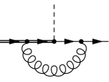
Figure 3: Subdiagram for $C$ and $E$.

References

- [1] J. Ellis, M. K. Gaillard, and D. V. Nanopoulos, Nucl. Phys. B106 (1976) 292.
- [2] A. I. Vaĭnshteĭn, M. B. Voloshin, V. I. Zakharov, and M. A. Shifman, Yad. Fiz. 30 (1979) 1368 [Sov. J. Nucl. Phys. 30 (1979) 711].
- [3] A. I. Vaĭnshteĭn, V. I. Zakharov, and M. A. Shifman, Usp. Fiz. Nauk. 131 (1980) 537 [Sov. Phys. Usp. 23 (1980) 429]; L. B. Okun, Leptons and Quarks, North-Holland, Amsterdam (1982), p. 229.
- [4] J. F. Gunion, H. E. Haber, G. Kane, and S. Dawson, The Higgs Hunter’s Guide, Addison-Wesley (1990).
- [5] S. Dawson, Nucl. Phys. B359 (1991) 283; A. Djouadi, M. Spira, and P. M. Zerwas, Phys. Lett. B264 (1991) 440.
- [6] B. A. Kniehl and M. Spira, Nucl. Phys. B432 (1994) 39.
- [7] B. A. Kniehl and M. Spira, Preprint DESY-95-008, hep-ph/9501392.
- [8] B. A. Kniehl and M. Spira, Preprint DESY 95-041, MPI 95-21, FERMILAB-PUB-95/081-T, hep-ph/9505225.
- [9] M. A. Shifman, Usp. Fiz. Nauk. 157 (1989) 561 [Sov. Phys. Usp. 32 (1989) 289].
- [10] B. Grzadkowski and J. Pawelczyk, Phys. Lett. B300 (1993) 387.
- [11] S. L. Adler, Phys. Rev. 177 (1969) 2416; S. L. Adler and W. A. Bardeen, Phys. Rev. 182 (1969) 1517; J. Bell and R. Jackiw, Nuovo Cim. 60A (1969) 47.
- [12] E. Kraus and K. Sibold, Preprint BONN-TH-95-04, MPI-Ph/95-11, hep-th/9503140.
- [13] S. Coleman, Dilatations, in: Aspects of Symmetry, Cambridge University Press (1985).
- [14] J. H. Lowenstein, Commun. Math. Phys. 24 (1971) 1; Y.-M. P. Lam, Phys. Rev. D6 (1972) 2145, D7 (1973) 2943; T. E. Clark and J. H. Lowenstein, Nucl. Phys. B113 (1976) 109.
- [15] C. G. Callan, Phys. Rev. D2 (1970) 1541; K. Symanzik, Commun. Math. Phys. 18 (1970) 227.
- [16] P. Breitenlohner and D. Maison, Commun. Math. Phys. 52 (1977) 11, 39, 55.
- [17] H. Georgi, Effective field theory, Annu. Rev. Nucl. Part. Sci. 43 (1993) 209, and references therein.
- [18] E. Kraus, Helv. Phys. Acta 67 (1994) 424.
- [19] J. Collins, Renormalization, Cambridge University Press (1984).
- [20] E. Kraus, Preprint BUTP-93/26, hep-th/9311158.