BGU-94/04
hep-ph/9505264

$FSI$ Corrections For Near Threshold Meson Production In Nucleon-Nucleon Collisions

Abstract

A procedure is proposed which accounts for final state interaction corrections for near threshold meson production in nucleon-nucleon scattering. In analogy with the Watson-Migdal approximation, it is shown that in the limit of extremely strong final state effects, the amplitude factorizes into a primary production amplitude and an elastic scattering amplitude describing a $3\to 3$ transition. This amplitude determines the energy dependence of the reaction cross section near the reaction threshold almost solely. The approximation proposed satisfies the Fermi-Watson theorem and the coherence formalism. Application of this procedure to meson production in nucleon-nucleon scattering shows that, while corrections due to the meson-nucleon interaction are small for s-wave pion production, they are crucial for reproducing the energy dependence of the $\eta$ production cross section.

PACS number(s) : 13.75.Cs, 14.40.Aq, 25.40.Ep

1 Introduction

The cross sections for $\pi^{0}$ and $\eta$ meson production via the $pp\to pp\pi^{0}$ and $pp\to pp\eta$ reactions, at energies near their respective thresholds, exhibit a pronounced energy dependence which deviates strongly from phase space[1, 2]. Such deviations, which occur in other hadronic collisions as well[3], are most certainly due to final state interactions($FSI$) between the reaction products. While $FSI$ corrections due to the short range nucleon-nucleon($NN$) force between the outgoing protons seem adequate to reproduce the observed energy dependence[1] and the cross section scale[4] for pion production, they fail to do so for the $\eta$ production[2]. Particularly, several model calculations[5, 6, 7] have considered the $NN\to NN\eta$ through a perturbative approach but none of them reproduced the energy dependence near threshold, although $FSI$ corrections were made to account for the proton-proton interaction. It is the purpose of the present work to show that while the meson-nucleon interaction influences s-wave pion production only slightly, its effects are crucial for reproducing the energy dependence of the $pp\to pp\eta$ reaction.

There exists no theory of final state effects in the presence of three strongly interacting particles and our first objective will be to develop a procedure that accounts for both the $NN$ and meson-$N$ forces. To accomplish this task we consider a production process, $ab\to cde$. A full dynamical theory of such a process would require the solution of two and three-body scattering problems. Particularly, in the Faddeev formalism[8] the full transition amplitude is decomposed as a sum of three terms depending on which of the three final particle pairs interacts last. The evaluation of these terms, the so called Faddeev amplitudes, requires the solution of a set of coupled integral equations. Such a procedure should resolve the problem at hand but, in view of the scarcity of knowledge about the $\eta N$ interaction it may turn to be unreliable and rather long and tedious to apply. In what follows we develop an approximation along exactly the lines of the Watson’s approach[9] for two body reactions, ${\it i.e.}$, we look for a separation of the energy dependence due to $FSI$ from those of the primary production amplitude. Such an approximation may prove useful and easy to apply in analyzing near threshold meson production data from $NN$ scattering.

According to the Watson-Migdal $FSI$ theory for two body processes[9], the energy dependence of the full transition amplitude is governed by rescattering of final state particles. The full transition amplitude is approximated by,

$$T_{if}\approx M^{(in)}_{if}\ t^{(el)}_{ff}\ \ ,$$ (1)

where the primary production amplitude, $M^{(in)}_{if}$, is assumed to be a smooth and slowly varying function of energy and $t^{(el)}_{ff}$ is taken as the $free$ two-body elastic scattering amplitude in the exit channel. Thus the energy dependence of the full matrix element is determined mostly by $t^{(el)}_{ff}$. A decomposition as such of the amplitude into a primary production amplitude and a subsequent $FSI$ correction term is meaningful only if $t^{(el)}_{ff}$ is sufficiently large so that $FSI$ dominate the reaction amplitude. This requires that the distortion of the final state wave function (i.e. the deviation from a simple product of free particle wave functions) or alternatively, the $sticking\ factor$ (i.e. the probability of the particles to find each other’s vicinity) in itself be proportional to $t^{(el)}_{ff}$. Albeit, the particles spend a great deal of time close together, as should be the case in particle production processes close to threshold. Otherwise, the distortion factor of the final state (and obviously the full matrix element) must be calculated by using more precise methods[9].

The complete transition amplitude of a production process can be decomposed in the form shown in fig. 1, where the first term (the block $M^{(in)}$) represents the primary production amplitude which includes all possible inelastic transitions contributing to the process, while all other terms represent the contributions from rescatterings in the entrance and exit channels (the $ISI$ and $FSI$ blocks). The third term, for example, corresponds to a process in which the primary production takes place as if there were no $FSI$ and only subsequently is distorted by the Coulomb and nuclear short range interactions between the reaction products. At energies near the reaction threshold, where the relative energies of particle pairs in the final state are sufficiently small and $FSI$ corrections are dominating, such a term is expected to be more important than others. In analogy to the Watson-Migdal approximation we make the $ansatz$ that in the limit of weak $ISI$ and strong $FSI$ , the transition amplitude of a three-body reaction can be approximated by an expression similar to eqn. 1, with the $FSI$ correction term being replaced by the on mass-shell $elastic$ scattering amplitude of a $3\to 3$ (three particles in to three particles out) transition. This amplitude is denoted by $T^{(el)}_{33}$ and, can be evaluated using the Faddeev formalism[10] or others such as the Weinberg method[11]. Certainly, it is not a measurable quantity as such a $3\to 3$ transition is not easy to realize experimentally. It is shown in sect. 2 though, that at energies near particle production threshold, $T^{(el)}_{33}$ can be estimated from two-body scattering data without having to solve the full three-body dynamics.

Within this approximation, the transition amplitude of a three-body reaction is coherent in terms of the interactions between the various final particle pairs, just as one anticipates based on general quantum mechanical considerations[12]. Thus the effects due to a given pair’s interaction is distributed over the entire transition amplitude and may influence strongly the energy dependence of the cross section. In sect. 3 we apply the procedure developed to production of mesons in $NN$ scattering and show that although the $\eta-N$ interaction is rather weak with respect to the $NN$ interaction it makes remarkably strong contributions. Discussion of the results and conclusions are given in sect. 4.

2 Theoretical Perspective

2.1 Two-body reactions

Prior to extending the Watson-Migdal approximation to three-body reactions let us recall first the more familiar problem of $FSI$ corrections in two-body reactions. Assume that the full interaction between particles separates into $v\ =\ w\ +\ s$, where $w$ and $s$ stand for weak and strong terms respectively. Here $w$ is the primary interaction, such that if it were zero, the process in question would not occur. The remaining part of the interaction $s$ is responsible for rescatterings in the entrance and exit channels. We further assume that $s$ is the only strong channel energetically allowed.

We would like to find how $FSI$ affects the transition amplitude in a process in which the primary interaction is relatively weak. The full transition amplitude in an appropriate eigenchannel is defined as,

$$T_{if}=\langle\Psi^{(-)}_{el,f}|\ \hat{M}^{(in)}_{if}\ |\Psi^{(+)}_{el,i}\rangle\ \ ,$$ (2)

where $\Psi^{(\pm)}_{el,i(f)}$ are two-particle scattering wave functions. They correspond to solutions of the Schr$\ddot{o}$dinger equation with a Hamiltonian that contains strong $s$-interactions only and satisfy the boundary conditions that $\Psi^{(+)}_{el,i}$ ($\Psi^{(-)}_{el,f}$) tends asymptotically to free two-particle wave function $\phi_{oi}$ ($\phi_{of}$), plus outgoing (ingoing) spherical waves. These can be written in the form[10],

$$\Psi^{(\pm)}_{el,\lambda}(E)=\lim_{\epsilon\to 0}\ [\ 1\ +\ G_{02}(E\pm i\epsilon)\ \hat{t}^{(el)}_{\lambda\lambda}]\ \phi_{0\lambda}\ \ ,\lambda=i,\ f\ \ .$$ (3)

Here $G_{02}(E\pm i\epsilon)$ is a free two-body Green’s functions, and $t^{(el)}_{ii}$ and $t^{(el)}_{ff}$ are two-body elastic scattering amplitude for the entrance and exit channels, respectively. Substituting eqn. 3 in 2 leads to the full transition amplitude,

$$\hat{T}_{if}=\hat{M}^{(in)}_{if}+\hat{t}^{(el)}_{ii}G_{02}\hat{M}^{(in)}_{if}+\hat{M}^{(in)}_{if}G_{02}\hat{t}^{(el)}_{ff}+\hat{t}^{(el)}_{ii}G_{02}\hat{M}^{(in)}_{if}G_{02}\hat{t}^{(el)}_{ff}\ \ .$$ (4)

Note that this expression is exact and contains both $ISI$ and $FSI$ . In the Watson-Migdal approximation,

$$T_{if}\approx\langle\Psi^{(-)}_{el,f}\ |\ \phi_{0f}\rangle\langle\ \phi_{0f}\ |\ \hat{M}^{(in)}_{if}\ |\phi_{0i}\rangle\langle\ \phi_{0i}|\Psi^{(+)}_{el,i}\rangle\ \ ,$$ (5)

where the two overlapping integrals $\langle\phi_{0i}|\Psi^{(+)}_{el,i}\rangle$ and $\langle\Psi^{(-)}_{el,f}\ |\ \phi_{0f}\rangle$ are on mass-shell $S$ matrix elements which contain $ISI$ and $FSI$ corrections, respectively. To cast the amplitude, eqn. 5, in the form given by the Watson’s approximation, eqn. 1, one has to replace $\Psi^{(+)}_{el,i}$ by $\phi_{0i}$ so that $S_{ii}$ is equal to unity and, in the limit of extremely strong $FSI$ , take the on mass-shell $t^{(el)}_{ff}$ instead of the $S_{ff}$ matrix elements.

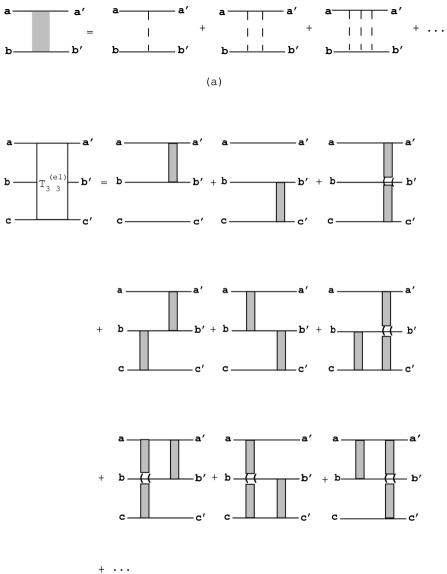
Figure 3: Graphical representation of elastic amplitudes: a) the amplitude $t^{(el)}_{22}$ for $ab\to ab$, b) the amplitude $T^{(el)}_{33}$ for $cde\to cde$; the blocks represent two-body scattering amplitudes in three-body space similar to the one defined in 3a.

It would be instructive to repeat these arguments using a diagrammatic language. We associate the weak primary interaction $w$ with the diagram $2a$, and the strong $s$ interaction with the diagram 2b of figure 2. As usual the disconnected diagram $2c$ describes noninteracting particles. It is evident that the amplitude $T_{if}$ is the sum of all diagrams that can be constructed from the elementary diagrams $2a$ and $2b$. To single out the $ISI$ and $FSI$ blocks and obtain the full matrix element in a diagrammatic representation similar to the one of fig. 1, we first sum in the initial and final channels all diagrams that contain strong interactions only (see fig. 3). These sums yield the elastic amplitudes $t^{(el)}_{\lambda\lambda}$ ($\lambda=i,\ f$) which we identify with the appropriate $ISI$ and $FSI$ blocks, respectively. The sum of all diagrams that start or end with a weak interaction (diagram $2a$) forms the block $M^{(in)}$ which describes the $primary$ production process. When rescatterings in both of the initial and final states give sufficiently large amplitudes, the Migdal-Watson ideology tells us that the 4th term on the rhs of eqn. 4 is dominating. When $FSI$ ($ISI$) effects are small, then the second (third) term dominates. Thus the $ISI$ and $FSI$ effects can be separated from the full transition amplitude by summing diagrams in a specific order and subsequently derive the Watson-Migdal approximation by selecting an appropriate dominant term in the limit of extremely weak $ISI$ and extremely strong $FSI$ . We apply this same reasoning to obtain the Watson-Migdal approximation for three-body reactions.

2.2 Three-body reactions

Let $T_{23}$ be the transition amplitude of a production process in which an initial two-body process goes into a final three-body state. For conciseness assume all particles to be distinguishable and spinless. This restriction simplifies the mathematics but can be easily removed to treat more general cases. Furthermore, assume that each pair in the three-body final state has a given angular momentum so that a unique elastic scattering state is assigned to each pair simultaneously. This is very often the case at energies near threshold where, only one partial wave dominates for each pair namely, $\lambda=0$. Following the discussion given above for two-body reactions the interactions are divided into two categories: (i) elastic interactions leading to rearrangement of particle (inner) quantum numbers but not to the production of any additional hadrons, (ii) inelastic interactions which are responsible for the production (or annihilation) of particles so that particle numbers in the initial and final states are different. Likewise, we call elastic those diagrams which involve elastic interactions only and having equal number of legs to the left hand and to the right hand sides. Those which begin and end with inelastic interactions and having different number of legs to the left and right hand sides are called inelastic.

The transition amplitude $T_{23}$ of the reaction under considerations is the sum of all diagrams which start with two legs on the left and end with three legs on the right, that can be assembled using all possible elastic and inelastic diagrams. To decompose $T_{23}$ into four terms as depicted in fig. 1, these diagrams need be organized in a specific order before suming them. First note that by summing all two-particle elastic diagrams in the entrance channel and all three-particle elastic diagrams in the exit channel, one obtains the $2\to 2$ and $3\to 3$ $elastic$ transition amplitude of fig. 3. These elastic amplitudes which are denoted by $t^{(el)}_{22}$ and $T^{(el)}_{33}$, contain only elastic interactions and as such, they are only parts of the complete $2\to 2$ and $3\to 3$ amplitudes. Although at energies above particle production threshold, two and three-particle channels may well be opened in both the initial and final states, these two amplitudes are calculated by taking into account only elastic interactions. All inelastic and quasi-elastic processes are confined into $M^{(in)}$. Note also, that the $2\to 2$ elastic block contains connected diagrams only but, the $3\to 3$ block contains disconnected diagrams as well (see fig. 3).

The set of all diagrams contributing to the entire transition amplitude $T_{23}$, is now separated into four partial sums each corresponding to one of the terms in the block diagram of fig. 1 : (i) the block $M^{(in)}$ is the sum of all inelastic diagrams only, (ii) the $ISI$ -$M^{(in)}$ term is the sum of all diagrams which start with a $2\to 2$ elastic diagram on the left and end with an inelastic diagram on the right, (iii) the $M^{(in)}$-$FSI$ term is the sum of all diagrams which start with an inelastic diagram on the left and end with a $3\to 3$ elastic diagram to the right and, (iv) the $ISI$ -$M^{(in)}$-$FSI$ term is the sum of all diagrams which start with a $2\to 2$ elastic diagram on the left and end with a $3\to 3$ elastic diagram on the right. Obviously, these four partial sums exhaust the entire set of diagrams that may contribute to the complete transition amplitude.

This same presentation of $T_{23}$ as the sum of the terms of fig. 1 can as well be derived formally. By definition, the transition amplitude is,

$$T_{23}=\langle\Psi^{(-)}_{el,3}|\hat{M}^{(in)}|\Psi^{(+)}_{el,2}\rangle\ \ ,$$ (6)

where as defined in eqn. 3, $\Psi^{(+)}_{el,2}$ stands for a two-body elastic scattering wave function and $\Psi^{(-)}_{el,3}$ is a three-particle elastic scattering wave function corresponding to the exit channel. It is a solution of a three-body Schr$\ddot{o}$dinger equation with a Hamiltonian having only two-body and three-body elastic interactions, and satisfies the boundary conditions that $\Psi^{(-)}_{el,3}$ tends asymptotically to a free three-particle wave function, $\phi_{03}$, plus outgoing spherical waves. In terms of the elastic scattering amplitudes defined above one has the expression[10],

$$\Psi^{(-)}_{el,3}=\lim_{\epsilon\to 0}\ [\ 1+G_{03}(E\ +\ i\epsilon)\ \hat{T}^{(el)}_{33}\ ]\ \phi_{03}\ \ .$$ (7)

Using this with eqn. 3 in eqn. 6 implies that,

$$\hat{T}_{23}=\hat{M}^{(in)}+\hat{t}^{(el)}_{22}\hat{G}_{02}\hat{M}^{(in)}+\hat{M}^{(in)}\hat{G}_{03}\hat{T}^{(el)}_{33}+\hat{t}^{(el)}_{22}\hat{G}_{02}\hat{M}^{(in)}\hat{G}_{03}\hat{T}^{(el)}_{33}\ \ .$$ (8)

Formally, this expression provides an exact solution of the problem and has a structure identical in form to that given in eqn. 4, for two-body reactions. A notable feature of this expression is that all inelastic transitions are confined in the block $M^{(in)}$, while all possible $elastic$ rescatterings in the entrance and exit channels are contained in $t^{(el)}_{22}$ and $T^{(el)}_{33}$.

Let us now consider $FSI$ corrections $a\ la\ Migdal-Watson$. In the limit of extremely weak $ISI$ one may replace $\Psi^{(+)}_{el,2}$ by $\phi_{02}$ in eqn. 6. This makes the second and fourth terms on the rhs of eqn. 8 disappear. Furthermore, in the limit of very strong $FSI$ the third term on the rhs of eqn. 8 dominates and we may approximate the transition amplitude by,

$$T_{23}\approx\langle\phi_{02}|\hat{M}^{(in)}|\phi_{03}\rangle\ T^{(el)}_{33}\ \ .$$ (9)

We may argue that the matrix element $\langle\phi_{02}|\hat{M}^{(in)}|\phi_{03}\rangle$ is a smooth and slowly varying function of the energy and momenta and hence the energy dependence of the amplitude, eqn. 9, is determined almost solely by the elastic amplitude $T^{(el)}_{33}$. Although in form eqn. 9 resembles the Watson-Migdal approximation for two-body reactions, eqn. 1, there exists an essential difference between the two cases which makes eqn. 9 more difficult to apply. This is because the amplitude $T^{(el)}_{33}$, contrary to $t^{(el)}_{ff}$, is practically not a measurable quantity.

The two-body initial state, $\Psi_{el,2}^{(+)}$, can be calculated using distorted wave approach and the effects of slowly varying nonvanishing $ISI$ can be included by replacing $M^{(in)}$ in eqn. 9 with the matrix element $\langle\phi_{03}|\hat{M}^{(in)}|\Psi^{(+)}_{el,2}\rangle$. With this modification in mind eqn. 9 is more suitable to apply to data. Certainly, $ISI$ must be included in a full dynamical description of the process as they influence the cross section scale through the matrix element $M^{(in)}$.

2.3 The amplitude for $3\to 3$

In the Faddeev formalism $T^{(el)}_{33}$ is written as a sum of three Faddeev amplitudes,

$$T^{(el)}_{33}=\sum_{j=1}^{3}T^{j}\ \ .$$ (10)

These satisfy the set of coupled integral equations[10],

$$T=t+FT=\sum_{n=0}^{\infty}\ (\ FF\ )^{n}\ [\ t+Ft\ ]\ \ ,$$ (11)

where we have used the notation,

$$T=\left(\begin{array}[]{c}T^{1}\\ T^{2}\\ T^{3}\\ \end{array}\right)\ \ ,t=\left(\begin{array}[]{c}t_{1}\\ t_{2}\\ t_{3}\\ \end{array}\right)\ \ ,F=\left(\begin{array}[]{clcr}0&t_{1}&t_{1}\\ t_{2}&0&t_{2}\\ t_{3}&t_{3}&0\\ \end{array}\right)G_{03}\ \ ,$$ (21)

and final particles are labeled 1,2 and 3. Here $t_{j}$ are two-body scattering amplitudes in the three-body space. In momentum space and adopt the convention that ($j,l,k$) are always cyclic,

$$\langle{\bf p}_{j},{\bf p}_{l},{\bf p}_{k}\ |\ t_{j}\ |\ {\bf p}_{j}^{\prime},{\bf p}_{l}^{\prime},{\bf p}_{k}^{\prime}\rangle=\langle{\bf p}_{l},{\bf p}_{k}\ |\ \hat{t}_{j}(E-\epsilon_{j})\ |\ {\bf p}_{l}^{\prime},{\bf p}_{k}^{\prime}\rangle\ \delta({\bf p}_{j}-{\bf p}_{j}^{\prime})\ \ ,$$ (22)

with $\hat{t}_{j}$ being a solution of the ordinary two-body Lippmann-Schwinger equation of the energy variable $E-\epsilon_{j}$. E is the total three-body energy and $\epsilon_{j}$ the energy appropriate to momentum ${\bf p}_{j}$. From the definitions in eqn. 12,

$$T^{j}=t_{j}\ +\ (T^{l}+T^{k})\ G_{03}\ t_{j}\ \ ,\ j\neq l\neq k\neq j\ \ ,\ \ j=1-3\ \ .$$ (23)

As pointed by Amado[12], the contributions from the various pair interactions add coherently and the effects of a given pair’s interactions is distributed over the entire amplitude. From eqn. 14, $T^{j}$ is the sum of all terms contributing to $T^{(el)}_{33}$ which end with $t_{j}$ but, it does not include all contributions of the $l-k$ interaction. Note that the first term on the rhs represents the $l-k$ two-body scattering amplitude with the $j$th particle being a spectator and as such it corresponds to a disconnected diagram. In the center of mass of the $l-k$ pair and for a given partial wave $\lambda$, $t_{j}$ has the elastic scattering phase $\delta_{\lambda}(j)$. The second term in eqn. 14 represents the contributions from two or more rescatterings and involves completely connected diagrams only. These play an important role in the coherence formalism[12] through interference with similar terms involving the $j-l$ and $j-k$ pair interactions. Therefore, in order to account for the effects of any pair’s interaction the entire amplitude must be constructed. Adding the sum ($T^{l}+T^{k}$) to $T^{j}$ of eqn. 14, one obtains three equivalent forms of the entire amplitude,

$$T^{(el)}_{33}=t_{j}+(T^{l}+T^{k})\ [1+G_{03}(E)\ t_{j}]\ ,\ j\neq l\neq k\neq j\ \ ,\ \ j=1-3\ \ .$$ (24)

In each of the forms in eqn. 15, there appears the factor ($1+G_{03}\ t_{j}$) with the $t_{j}$ being half on-shell. At a given $l-k$ relative momentum (${\bf q}_{j}$) in a given $l-k$ partial wave ($\lambda$) and following the arguments in ref.[12], these half-on-shell amplitudes, the factor ($1+G_{03}\ t_{j}$) and, the entire amplitude have the phase $\delta_{\lambda}$(j). For this to happen, say in a region where the expression $(T^{l}\ +\ T^{k})\ G_{03}\ t_{j}$ may vary rapidly with energy it must have a part which cancels the variation of $(T^{l}\ +\ T^{k})$ so as to give to their sum the behaviour of $t_{j}$. This general observation on three-body amplitudes, which is true for $T_{23}$ as well as for $T_{33}$, has far reaching consequences on the energy dependence of the entire amplitude. Certainly, in order to take this cancelation into account the terms corresponding to completely connected diagrams must be included.

Another general constraint on the form of $T_{23}$ is provided by the so called Fermi-Watson theorem. This requires that the phase of the transition amplitude of the entire amplitude is determined by the phases and norms of the rescattering amplitudes in the entrance and exit channel and that in the limit of vanishing $ISI$ the overall phase of the entire amplitude is equal to that of the elastic scattering amplitude in the exit channel. This well established for two-body reactions[13] is easily extended to the case of three-body reactions near threshold (see Appendix A). Explicitly, for the case under considerations, this theorem requires that the phase of $T_{23}$ must be identical to the overall phase of $T^{(el)}_{33}$. Both of these constraints are satisfied by the approximation, eqn. 9, in a natural way.

Turning now to estimate the rescattering amplitude, we note first that the kernel $FF$ is compact for any complex E and therefore eqns. 11 has a unique solution. By solving these equations by iteration , one can calculate the amplitude $T^{(el)}_{33}$ with the required accuracy. To first order $T^{(el)}_{33}\ \approx\ [\ t\ +\ Ft\ ]$. It is the sum of all diagrams shown in fig. 3b. The first three of these are disconnected and represent the contributions of the free $t$. As shown by Amado[12] and Cahill[14] taking the sum of just these three diagrams would not yield a coherent amplitude and therefore would not be a satisfactory solution. The other diagrams of fig. 3b give the first order correction due to two subsequent elastic scatterings, they are all completely connected and as indicated above play an important role in the coherence mechanism[12, 14]. The next iteration introduces connected diagrams with three and four rescatterings and so on. Summing the contributions of diagrams up to the corresponding order leads, in principio, to $T^{(el)}_{33}$ with the accuracy required.

As a first step we restrict the following discussion to $FSI$ corrections due to one and two rescattering diagrams only (fig. 3b), i.e. , we calculate $T^{(el)}_{33}$ to first order only. Denoting contributions from double scattering diagrams by $C_{jl}$ it is shown in Appendix B that for s-wave production at energies close to threshold,

$$C_{jl}=M^{(in)}(0,0)\ q_{j}\ t^{(on)}_{j}(0,\frac{q_{j}^{2}}{2\mu_{j}})\ t^{(on)}_{l}(0,\frac{q_{l}^{2}}{2\mu_{l}})\ I_{jl}\ \ .$$ (25)

where $I_{jl}$ are integrals of Kowalski-Noyes[15] half-shell functions over the appropriate relative momenta of the interacting pairs. Thus the entire transition amplitude can be written as,

$$T_{23}\approx M^{(in)}_{23}(0,0)\ Z_{33}\ \ ,$$ (26)

where the $FSI$ correction factor is given by,

$$Z_{33}=\sum_{j=1}^{3}t^{(on)}_{j}(0,\frac{q_{j}^{2}}{2\mu_{j}})\ +\sum_{j,l=1}^{3}q_{j}\ t^{(on)}_{j}(0,\frac{q_{j}^{2}}{2\mu_{j}})\ t^{(on)}_{l}(0,\frac{q_{l}^{2}}{2\mu_{l}})\ I_{jl}\ \ .$$ (27)

A further simplification can be achieved by setting all $I_{jl}$ equal unity, thus neglecting off shell effects (see Appendix B). This allows calculating the $FSI$ factor from two-body scattering data of the particles involved. To evaluate $T^{(el)}_{33}$ to second order we need to include $(\ FF\ )\ [\ t\ +\ Ft\ ]$ terms. The evaluation of such terms is described in Appendix C, where it is shown that the effect of the (FF) factor is to scale the first order amplitude $[\ t\ +\ Ft\ ]$ by,

$$\langle\ FF\ \rangle \approx q_{k}\ t^{(on)}_{k}(0\ ,\frac{q^{2}_{k}}{2\ \mu_{lj}})\ q_{l}\ t^{(on)}_{l}(0\ ,\frac{q^{2}_{l}}{2\ \mu_{jk}})$$

$$\approx \exp{i(\ \delta_{k}\ +\ \delta_{l})}\sin{\delta_{k}}\sin{\delta_{l}}\ \ .$$

Here we have used the standard parameterization,

$$t(q,q)=\frac{1}{q(\cot{\delta}-i)}\ \ ,$$ (29)

with the $\delta$’s being the appropriate s-wave phase shifts. These are related to the s-wave scattering length according to,

$$|\langle\ FF\ \rangle| \approx \sin\delta_{k}\sin\delta_{l}=\frac{q_{k}\ a_{k}\ q_{l}\ a_{l}}{(1\ +\ q_{k}\ a_{k})(1\ +\ q_{l}\ a_{l})}\ \ .$$ (30)

Thus in case of $q_{k}\ a_{k}\ q_{l}\ a_{l}\ll 1$ , the factor $\langle\ FF\ \rangle\ll 1$ so that the evaluation of $T^{(el)}_{33}$ to first order should be sufficient.

3 Application

In the present section we apply the procedure described above to analyze the effects of $FSI$ on the energy dependence of $\pi$ and $\eta$ meson production in $NN$ scattering at energies near their respective production thresholds. We demonstrate this first for $\pi$ meson production. For the $pp\to pp\pi^{0}$ reaction, rescatterings may include the following sequences : $pp\to pp\pi^{0}\to pp\pi^{0}$, $pp\to pn\pi^{+}\to pp\pi^{0}$ and $pp\to d\pi^{+}\to pp\pi^{0}$. In considering $FSI$ only the first sequence is included as by definition the block $FSI$ includes $elastic$ interactions only. Two-nucleon mechanism contributions dominate the $pp\to pp\eta$ cross section and any reasonable calculations of the primary amplitude must include $\pi^{+}$ production followed by charge exchange. The effects of these other channels are assumed to be absorbed in $M^{(in)}$. The isosinglet and isotriplet pion-nucleon scattering amplitudes are calculated from eqn. 20, using the isosinglet and isotriplet pion nucleon scattering length values $a_{1}=0.245fm$ and $a_{3}=-0.143fm$ of ref.[16]. The isospin average scattering length of these values is rather small so that $a\ priori$ the overall $\pi$N interaction effects on the energy dependence are expected to be very small. Similarly, the S-wave $pp$ phase shift is obtained from effective range expansion using the modified Cini-Fubini-Stanghellini formula[17],

$$C^{2}\ q\ ctn\ \delta+2\eta_{c}qh(\eta_{c})=-\frac{1}{a_{pp}}+\frac{1}{2}r_{pp}q^{2}-\frac{p_{1}\ q^{4}}{1\ +\ p_{2}k^{2}}\ \ ,$$ (31)

where $a_{pp}$ and $r_{pp}$ denote the $pp$ scattering length and effective range and,

$$\eta_{c}=\frac{e^{2}E_{lab}}{P_{lab}}\ \ ,C^{2}=\frac{2\pi\ \eta_{c}}{(\exp{2\pi\eta_{c}}-1)}\ \ ,h(\eta_{c})=\sum_{s=1}^{\infty}\frac{\eta_{c}^{2}}{s(s^{2}+\eta_{c}^{2})}-\gamma-\ln{\eta_{c}}\ \ .\\$$ (32)

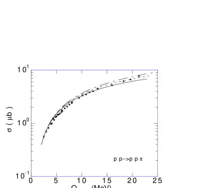
Figure 5: The $\pi$ meson production cross section $vs.$ the energy available in the $cm$ system, $Q_{cm}$. The predictions with the full $FSI$ correction factor of eqns. 20 are shown as the solid line. Those without the meson-nucleon interaction and with the disconnected diagrams of fig. 3b are given by the large-dashed and small-dashed lines, respectively. All curves are normalized to the lowest data point.

The $p_{i}$ (i=1,2) are functions of $a_{pp}$ and $r_{pp}$. In what follows we have used the values $a_{pp}=-7.82fm$ and $r_{pp}=2.7fm$ of ref.[17]. To calculate the cross section, the $FSI$ factor $|Z_{33}|^{2}$, eqn. 18, is multiplied by the invariant phase space and then integrated over the appropriate momenta. The primary production amplitude is assumed to be constant and is taken outside the integral. The energy dependence of the cross section as obtained with the $FSI$ factor calculated to first and second orders are displayed in fig. 4 as a function of $Q_{cm}$, the energy available in the $cm$ system. The two solutions are practically identical. The $\langle\ FF\ \rangle$ factor discussed in the previous section, is indeed very small so that the sum in eqn. 18 converges and it is safe to compare data with the predictions corresponding to first order calculations of $|Z_{33}|^{2}$. Comparison with data is made in fig. 5. The predictions with the full $FSI$ correction of eqn. 18 are shown as the solid line. Those without the $\pi N$ interaction and with only the first disconnected diagrams of fig. 3b are given by the large-dashed and small-dashed lines, respectively. The data in the figures are taken from ref.[1]. The curves are arbitrarily normalized to the lowest energy data point available. As indicated above the s-wave $\pi N$ interaction is relatively weak so that the $FSI$ correction factor is dominated by the strong interaction of the ${}^{1}S_{0}$ NN system. Our predictions with the full $FSI$ correction factor (solid curve) agrees slightly better with data compared with those obtained by including the $NN$ force only (dashed line). Nonetheless, even in this case, where the overall meson-nucleon interaction is weak, the effects from disconnected and completely connected diagrams are comparable. It is our contention that the completely connected diagrams of fig. 3b must be included if one wishes to interpret the recent precision measurements of $\pi$ production cross section[1, 4]. As demonstrated below the importance of these completely connected diagrams becomes more apparent in applying our procedure to $\eta$ production.

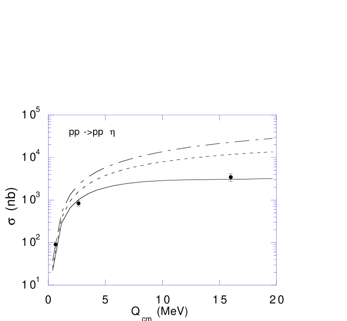
Figure 6: The $\eta$ meson production cross section $vs.$ $Q_{cm}$. The $\eta N$ scattering length is taken from ref. [18]. (see captions of fig. 5)

For $\eta$ meson production there are no direct measurements of elastic $\eta N$ scattering and the information available are extracted indirectly using $\pi N\to\eta N$ data. Based on $\pi N$ and $\eta N$ coupled channel analysis around the $\eta N$ threshold within an isobar model, Bhalerao and Liu[18] suggest a value $a_{\eta N}=(0.27+i0.22)\ fm$ for the $\eta N$ scattering length. With this choice of $a_{\eta N}$ the results of our analysis with the $FSI$ factor calculated to first order are shown in fig. 6. Here as for pion production, the solution with the $FSI$ factor calculated to second order is nearly identical. In contrast with $\pi$ production, this process is strongly influenced by the $\eta N$ interaction giving rise to a sharp enhancement of the cross section very near threshold and thus reproduces, rather accurately, the energy dependence of the cross section up to $Q_{cm}=20MeV$. Note also, that in the analysis presented above, the enhancement factor $|Z_{33}|^{2}$ is exactly what is required to keep the primary production amplitude nearly constant over the energy range from threshold to $Q_{cm}=20MeV$.

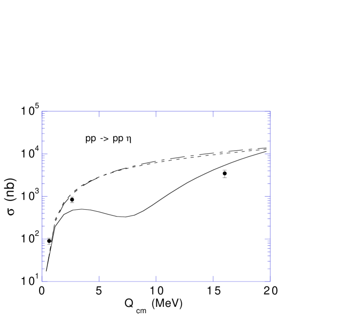
Figure 7: The $\eta$ meson production cross section $vs.$ $Q_{cm}$. The $\eta N$ scattering length is taken from ref. [3] (see captions of fig. 5)

It is interesting to explore how sensitive the results are for a different choice of the $a_{\eta N}$ scattering length. Since other channels such as the $\pi\pi N$ are also opened, Wilkin[3] has fixed the imaginary part to be $\Im[a_{\eta N}]=0.30fm$ and used the $\pi^{-}p\to\eta p$ data directly to determine the real part. This procedure has yielded a scattering length $a_{\eta N}=(0.55\pm 0.20+i0.30)\ fm$. Calculations with this value are given in fig. 7. The energy dependence is mostly sensitive to the real part of $a_{\eta N}$ and the results from our analysis do not support the $central$ value proposed by Wilkin[3]. It is to be noted also, that based on partial wave unitarity relations, an analysis of the $\pi^{-}p$ backward differential cross section data yields a value of $39^{o}.3\pm 4^{o}.7$ for the phase of the $\eta N$ production amplitude[19] a value in agreement with Bhalerao and Liu[18] but not with Wilkin[3].

4 Summary And Conclusions

In summary we have developed an approximate procedure which accounts for final state effects in the presence of three strongly interacting particles. In analogy with the Watson’s treatment[9] it was shown that, in the the limit of extremely strong $FSI$ the amplitude factorizes into a primary production amplitude and an elastic scattering amplitude describing a $3\to 3$ transition. The energy dependence of the cross section in the near vicinity of the reaction threshold is determined almost entirely by $T^{(el)}_{33}$. Based on the coherence formalism of Amado[12] we argue that the completely connected diagrams corresponding to two rescatterings may interfere strongly and therefore, play an important role in determining the energy dependence of the cross section. In view of the scarcity of knowledge about the meson-nucleon force, the approximation is particularly useful near threshold where $T^{(el)}_{33}$ can be estimated using nucleon-nucleon and meson-nucleon scattering data. Because of the strong NN force the $FSI$ term dominates. Detailed analysis of $\pi$ and $\eta$ production via $NN$ collisions show that the energy dependence of the cross section can be explained in both cases, by taking into account the meson-$N$ interaction also.

In the present analysis we have not considered $ISI$ corrections as these vary slowly with energy and would have little influence on the energy dependence. For $NN$ scattering at bombarding energies of several 100 MeV and above, the nuclear and Coulomb distortions are expected to be very small. The Gamov factor which accounts for Coulomb distortions is equal unity within 2.5$\%$ even for the pion data analyzed above. As previously mentioned $ISI$ effects can be included exactly by using distorted waves for the incoming two-proton state.

Finally, the primary production amplitude is not treated explicitly so that the cross section scale was arbitrary. This deficiency can be removed by incorporating in eqn. 17 a primary production amplitude from one of the existing perturbative models[5, 6, 7]. Such model calculations were performed for $\eta$ production, taking the $\eta$N interaction in the primary amplitude to be consistent with that occurring in the $FSI$ . They are found to reproduce the energy dependence as well as the scale of the cross section and will be published elsewhere[20].

In view of the large effects due to the $\eta N$ force the analysis presented above could well be used to study the $\eta N$ force itself for which no direct experiments are possible.

Appendix A

The Fermi-Watson theorem[13] can be extended to three-body reactions by applying unitarity. Let $T_{23}$ denotes the entire amplitude and let $t^{(el)}_{22^{\prime}}$ and $T^{(el)}_{3^{\prime},3}$ denote elastic $2\to 2$ and $3\to 3$ amplitudes, respectively. Then by unitarity,

$$\Im\{T_{23}\}=-\pi\sum_{2^{\prime}}t^{(el)}_{22^{\prime}}\delta(E-E_{2^{\prime}})T^{\dagger}_{2^{\prime}3}-\pi\sum_{3^{\prime}}T_{23^{\prime}}\delta(E-E_{3^{\prime}})T^{(el)\dagger}_{3^{\prime}3}\ \ .$$ (33)

The $\delta$ functions force the two body and three body elastic scattering amplitudes, $t^{(el)}_{22^{\prime}}$ and $T^{(el)}_{3^{\prime}3}$ to be on mass-shell.

In angular momentum representation the amplitudes of eqn. 24 can be written in the form,

$$T_{ij}=|T_{ij}|\exp{i\delta_{ij}}\ \ .$$ (34)

Note that $\delta_{2^{\prime}2}$ stands for two-body phase shift but $\delta_{3^{\prime}3}$ is only related to two-body phase shifts of the three interacting pairs and in itself is not a measurable quantity. Then substituting these into the unitarity condition, eqn. 24, leads to the following constraint on the $\delta$’s,

$$\Im\{|T_{23}|\exp{i\delta_{23}}\} = -\pi\sum_{2^{\prime}}|T^{(on)}_{22^{\prime}}||T^{(on)}_{2^{\prime}3}|\exp{i(\delta_{22^{\prime}}-\delta_{2^{\prime}3})}$$ (35)

$$-\pi\sum_{3^{\prime}}|T^{(on)}_{23^{\prime}}||T^{(on)}_{3^{\prime}3}|\exp{i(\delta_{23^{\prime}}-\delta_{3^{\prime}3})}\ \ .$$

In the case of a single channel with the angular momenta of the final pairs being zero, the phase $\delta_{23}$ from eqn. 26 is,

$$\sin{\delta_{23}} = {|t^{(on)}_{22}|\sin{\delta_{22}}-|T^{(on)}_{33}|\sin{\delta_{33}}}/$$ (36)

$$[|t^{(on)}_{22}|^{2}+|T^{(on)}_{33}|^{2}-2|t^{(on)}_{22}||T^{(on)}_{33}|\cos{(\delta_{33}-\delta_{22})}]^{1/2}\ \ .$$

Thus the phases of the rescattering amplitudes and their norms, determine the overall phase of the $2\to 3$ transition amplitude, just as the case is for a two body reactions. In the limit of very weak $ISI$ (vanishing $t^{(el)}_{22}$),

$$\sin{\delta_{23}}\approx\sin{\delta_{33}}\ \ ,$$ (37)

so that the overall phase of $T^{(el)}_{23}$ becomes identical to that of the elastic scattering amplitude $T^{(el)}_{33}$. Furthermore, the amplitudes and phases of the strong rescatterings in the entrance and exit channels are related through eqn. 26 by,

$$|t^{(el)}_{22}|\ (\sin{\delta_{22}}+\pi\ |t^{(el)}_{22}|)=|T^{(el)}_{33}|\ (\sin{\delta_{33}}+\pi\ |T^{(el)}_{33}|)\ \ .$$ (38)

For a real production process the amplitudes $t^{(el)}_{22}$ and $T^{(el)}_{33}$ must be independent so that the lhs and rhs of eqn. 27 must be equal to a constant. In the limit of very weak $ISI$ this constant must vanish so that,

$$|T^{(el)}_{33}|=\sin{\delta_{33}}/\pi\ \ .$$ (39)

Formally, this is identical in form to the expression assumed by Watson[9] for two-body processes.

Appendix B

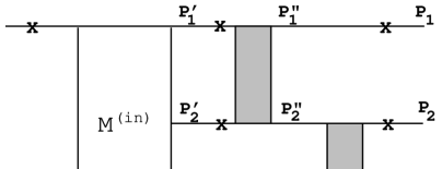
Figure 8: Typical completely connected diagram with two subsequent rescatterings. Crossed lines denote on mass-shell states.

We evaluate the contribution of diagrams with two rescatterings. As an example consider the diagram shown in fig. 8 (crossed lines denote on mass-shell states). In the CM system, in each of the three-body states of the diagram, there are only two independent momenta which are taken to be ${\bf p}_{j}$ the momentum of particle $j$ and ${\bf q}_{j}$ the relative momentum of the remaining $l-k$ pair. Adopting the convention that $(j,l,k)$ are always cyclic, ${\bf q}_{j}$ is defined as

$${\bf q}_{j}=\frac{(m_{k}{\bf p}_{l}-m_{l}{\bf p}_{k})}{(m_{l}+m_{k})}\ \ .$$ (40)

In terms of these momenta the total kinetic energy is ,

$$H_{0}=\frac{p^{2}_{j}}{2\mu_{j}}+\frac{q^{2}_{j}}{2\mu_{lk}}\ \ .$$ (41)

Here $\mu_{lk}$ is the reduced mass of the $l$ and $k$ particles and $\mu_{j}$ is the reduced mass of the $j$ particle, i.e. ,

$$\mu_{lk}=\frac{m_{l}m_{k}}{(m_{l}+m_{k})}\ \ ;\ \mu_{j}=\frac{m_{j}(m_{l}+m_{k})}{(m_{j}+m_{l}+m_{k})}\ \ .$$ (42)

Now the contribution of the diagram, fig. 8, can be written in the form,

$$C_{31} = \int d{\bf p}_{3}^{\prime}d{\bf q}_{3}^{\prime}\delta(E-\frac{p_{3}^{\prime 2}}{2\mu_{3}}-\frac{q_{3}^{\prime 2}}{2\mu_{12}})M^{(in)}({\bf p}_{3}^{\prime},{\bf q}_{3}^{\prime})$$

$$\int d{\bf p}_{1}^{\prime\prime}d{\bf q}_{1}^{\prime\prime}\delta({\bf p}_{3}^{\prime}-{\bf p}_{3}^{\prime\prime})t_{3}({\bf q}_{3}^{\prime},{\bf q}_{3}^{\prime\prime};E^{+}-\frac{p_{3}^{\prime\prime 2}}{2\mu_{3}})$$

$$[E^{+}-\frac{p_{1}^{\prime\prime 2}}{2\mu_{1}}-\frac{q_{1}^{\prime\prime 2}}{2\mu_{23}}]^{-1}\delta({\bf p}_{1}^{\prime\prime}-{\bf p}_{1}))t_{1}({\bf q}_{1}^{\prime\prime},{\bf q}_{1};E^{+}-\frac{p_{1}^{2}}{2\mu_{1}})\ \ .$$

The integration over ${\bf p}_{1}^{\prime\prime}$ and ${\bf p}_{3}^{\prime}$ are immediate and we obtain,

$$C_{31} = \int d{\bf q}_{3}^{\prime}\delta(E-\frac{p_{3}^{\prime\prime 2}}{2\mu_{3}}-\frac{q_{3}^{\prime 2}}{2\mu_{12}})M^{(in)}({\bf p}_{3}^{\prime\prime},{\bf q}_{3}^{\prime})$$

$$\int d{\bf q}_{1}^{\prime\prime}t_{3}({\bf q}_{3}^{\prime},{\bf q}_{3}^{\prime\prime};E^{+}-\frac{p_{3}^{\prime\prime 2}}{2\mu_{3}})$$

$$[E^{+}-\frac{p_{1}^{2}}{2\mu_{1}}-\frac{q_{1}^{\prime\prime 2}}{2\mu_{23}}]^{-1}t_{1}({\bf q}_{1}^{\prime\prime},{\bf q}_{1};E^{+}-\frac{p_{1}^{2}}{2\mu_{1}})\ \ .$$

Here $t_{3}$ is a half off mass-shell two-body matrix element with only the ${\bf q}_{3}^{\prime\prime}$ being off-shell momentum. (From a view point of invariant perturbation theory only one leg of $t_{j}$ is off mass-shell so that it behaves like a particle form-factor). Expanding $t_{j}$ in partial waves and introducing the Kowalski-Noyes half-shell function[15] $f_{j}(\lambda,{\bf q}_{j},{\bf q}^{\prime\prime})$ allows writing these for a partial wave $\lambda$ as,

$$t_{j}(\lambda,{\bf q}_{j},{\bf q}_{j}^{\prime\prime};E^{+})=t^{(on)}_{j}(\lambda,q^{2}_{j}/2\mu_{j})\ f_{j}(\lambda,{\bf q}_{j},{\bf q}_{j}^{\prime\prime})\ \ .$$ (45)

Then for slowly varying $M^{(in)}$ and at energies near threshold one obtains,

$$C_{31}=M^{(in)}(0,0)\ q_{3}\ t^{(on)}_{3}(0,\frac{q_{3}^{2}}{2\mu_{12}})\ t^{(on)}_{1}(0,\frac{q_{1}^{2}}{2\mu_{23}})\ I_{31}\ \ ,$$ (46)

where $I_{31}$ is an integral over the Kowalski-Noyes half-shell functions,

$$I_{31}=\frac{1}{(2\pi)^{2}\ \mu_{23}\ q_{3}}\int d{\bf q}_{1}^{\prime\prime}f_{3}(0,{\bf q}_{3},{\bf q}_{3}^{\prime\prime})[E-\frac{p^{2}_{1}}{2\mu_{1}}-\frac{q^{\prime\prime 2}_{1}}{2\mu_{23}}]^{-1}f_{1}(0,{\bf q}_{1},{\bf q}_{1}^{\prime\prime})\ \ ,$$ (47)

where,

$${\bf q}_{3}^{\prime\prime}=-\frac{m_{1}}{m_{1}+m_{2}}{\bf q}_{1}^{\prime\prime}-\frac{m_{2}(m_{1}+m_{2}+m_{3})}{(m_{1}+m_{2})(m_{1}+m_{3})}{\bf p}_{1}\ \ .$$ (48)

If we neglect off mass-shell effects the integrals $I_{jl}$ reduce to unity.

Appendix C

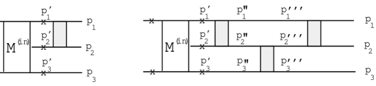
Figure 9: An example of diagrams contributing to the $T^{(el)}_{33}$ amplitude to second order : (a) a disconnected diagram which contributes to first order, (b) a completely connected diagram obtained from diagram (a) with the FF factor (see text).

We consider here second order contributions to the transition amplitude. As indicated in the text these are obtained by multiplying first order contributions with a factor (FF). We attempt demonstrating this for the diagram shown in Fig. 9. This can be written as,

$$D_{313} = \int d{\bf p}_{3}^{\prime}\ d{\bf q}_{3}^{\prime}\ d{\bf p}_{1}^{\prime\prime}\ d{\bf q}_{1}^{\prime\prime}\ d{\bf p}_{3}^{\prime\prime\prime}\ d{\bf q}_{3}^{\prime\prime\prime}\ \delta(E-\frac{p_{3}^{\prime 2}}{2\mu_{3}}-\frac{q_{3}^{\prime 2}}{2\mu_{12}})$$

$$M^{(in)}({\bf p}_{3}^{\prime},{\bf q}_{3}^{\prime})\ t_{3}({\bf q}_{3}^{\prime},{\bf q}_{3}^{\prime\prime};E^{+}-\frac{p_{3}^{\prime 2}}{2\mu_{3}})\ \delta({\bf p}_{3}^{\prime}-{\bf p}_{3}^{\prime\prime})\$$

$$[E^{+}-\frac{p_{1}^{\prime\prime 2}}{2\mu_{1}}-\frac{q_{1}^{\prime\prime 2}}{2\mu_{23}}]^{-1}\ \delta({\bf p}_{1}^{\prime\prime}-{\bf p}_{1}^{\prime\prime\prime})\ t_{1}({\bf q}_{1}^{\prime\prime},{\bf q}_{1}^{\prime\prime\prime};E^{+}-\frac{p_{1}^{\prime\prime\prime 2}}{2\mu_{1}})$$

$$[E^{+}-\frac{p_{3}^{\prime\prime\prime 2}}{2\mu_{3}}-\frac{q_{3}^{\prime\prime\prime 2}}{2\mu_{12}}]^{-1}\ \delta({\bf p}_{3}^{\prime\prime\prime}-{\bf p}_{3})\ t_{3}({\bf q}_{3}^{\prime\prime\prime},{\bf q}_{3};E^{+}-\frac{p_{3}^{2}}{2\mu_{3}})\ \ .$$

Integrating over ${\bf p}_{3}^{\prime}$, ${\bf p}_{1}^{\prime\prime}$ and ${\bf p}_{3}^{\prime\prime\prime}$ and arranging terms leads to,

$$D_{313} = {\Huge\{}\ q_{1}\ t^{(on)}_{1}(0\ ,\ \frac{q_{1}^{\prime\prime\prime 2}}{2\mu_{23}})\ q_{3}\ t^{(on)}_{3}(0\ ,\ \frac{q_{3}^{2}}{2\mu_{12}})\ \frac{1}{q_{1}\ q_{3}}\ \int d{\bf q}_{1}^{\prime\prime}\frac{1}{[E^{+}-\frac{p_{1}^{\prime\prime\prime 2}}{2\mu_{1}}-\frac{q_{1}^{\prime\prime 2}}{2\mu_{23}}]}$$

$$\int d{\bf q}_{3}^{\prime\prime\prime}\frac{f_{1}(0,{\bf q}_{1}^{\prime\prime},{\bf q}_{1}^{\prime\prime\prime})\ f_{1}(0,{\bf q}_{3}^{\prime\prime\prime},{\bf q}_{3})}{[E^{+}-\frac{p_{3}^{2}}{2\mu_{1}}-\frac{q_{3}^{\prime\prime\prime 2}}{2\mu_{12}}]}\ {\Large\}}$$

$$\int d{\bf q}_{3}^{\prime}\ M^{(in)}({\bf p}_{3}^{\prime},{\bf q}_{3}^{\prime})\ \delta(E-\frac{p_{3}^{\prime\prime 2}}{2\mu_{3}}-\frac{q_{3}^{\prime 2}}{2\mu_{12}})t_{3}(0,\frac{q_{3}^{\prime 2}}{2\mu_{12}})f_{3}(0,{\bf q}_{3}^{\prime},{\bf q}_{3}^{\prime\prime})\ \ .$$

We now notice that the last integral is the first order contribution from the disconnected diagram (9.a) with a single scattering block between particles 1 and 2 while the expression in the curly bracket is just the (FF) factor. An order of magnitude of this factor can be obtained using on mass-shell values for the Kowalski-Noyes functions. This leads to,

$$\langle\ FF\ \rangle\approx q_{1}\ t^{(on)}_{1}(0\ ,\ \frac{q_{1}^{\prime\prime\prime 2}}{2\mu_{23}})\ q_{3}\ t^{(on)}_{3}(0\ ,\ \frac{q_{3}^{2}}{2\mu_{12}})\ \ .$$ (51)

Similar expressions can be calculated for the completely connected diagrams (3.b) as well.

Acknowledgments This work was supported in part by Israel Ministry Of Science and Technology and the Israel Ministry Of Absorption. One of us ( A. M. ) thanks C. Wilkin for suggestions and stimulating discussions concerning the results reported in this work.

Figure 1: Graphical representation of the transition amplitude. The block $M^{(in)}$ represents the primary production mechanism of the reaction and contains all possible inelastic transitions from a two-particle state to a three-particle state (see text). The $ISI$ and $FSI$ blocks represent elastic rescattering in the entrance and exit channels, respectively.

Figure 2: Elementary inelastic(2a) and elastic(2b) interactions. A wavy line represents the primary interaction, such that if it were zero the reaction $ab\to cd$ would not occur. A dotted line represents an elastic interaction. The disconnected diagram(2c) describes non-interacting particles.

Figure 4: The $pp\to pp\pi^{0}$ cross section $vs.$ the energy available in the $cm$ system, $Q_{cm}$. The solid line represents predictions with the $FSI$ correction factor calculated to first ($T_{33}^{(el)}\approx[t+Ft]$). The dashed line is that obtained with the $FSI$ taken to second order,$i.e.$, $T_{33}^{(el)}\approx(1+FF)[t+Ft]$ (see text).

References

- [1] H. O. Meyer et al. , Nucl. Phys. , 633(1992).
- [2] A. M. Bergdolt et al., Phys. Rev. , R2969(1993).
- [3] C. Wilkin, Phys. Rev. , 938(1993); and private communications.
- [4] T. -S. H. Lee and D. O. Riska, Phys. Rev. Lett. , 2237(1993).
- [5] J. F. Germond and C. Wilkin, Nucl. Phys. , 308(1990); and refs. therein.
- [6] J. M. Laget, F. Wellers, and J. F. Lecolley, Phys. Lett. , 254(1991), and references therein.
- [7] T. Vetter, A. Engel, T. Biro, and U. Mosel, Phys. Lett. , 153(1991).
- [8] L. D. Faddeev, (Daniel Davey and Co., Inc., New York 1965).
- [9] M. Goldberger and K. M. Watson, (New York, Wiley, 1964).
- [10] I. R. Afnan and A. W. Thomas, in , Edited by A. W. Thomas (Springer-Verlag Berlin Heidelberg 1977).
- [11] Steven Weinberg, Phys. Rev. , B232(1964).
- [12] R. D. Amado, Phys. Rev. , 1414(1967); see also author’s contribution in ref. 10.
- [13] C. J. Joachain, (North-Holland Publication Company, 1975).
- [14] R. T. Cahill, Phys. Rev. , 1414(1974).
- [15] K. L. Kowalski, Phys. Rev. Lett. , 798(1965); H. P. Noyes, Phys. Rev. Lett. , 538(1965).
- [16] T. Ericson and W. Weise, (Clarendon Press . Oxford, 1988).
- [17] H. P. Noyes, Ann. Rev. Nucl. Sci., , 465(1972).
- [18] R. S. Bhalerao and L. C. Liu, Phys. Rev. Lett. , 865(1985).
- [19] Ramesh Bhandari and Yung-An Chao, Phys. Rev. , 192(1977).
- [20] A. Moalem, E. Gedalin, L. Razdolskaja and Z. Shorer, submitted for publication in Nucl. Phys. .