TTP95-10
March 1995
hep-ph/9505262

RADIATION OF LIGHT FERMIONS IN HEAVY FERMION PRODUCTION
A.H. Hoang, J.H. Kühn and T. Teubner
Institut für Theoretische Teilchenphysik, Universität Karlsruhe,

D–76128 Karlsruhe, Germany

Abstract
The rate for the production of a pair of massive fermions in $e^{+}e^{-}$ annihilation plus real or virtual radiation of a pair of massless fermions is calculated analytically. The contributions for real and virtual radiation are displayed separately. The asymptotic behaviour close to threshold and for high energies is given in a compact form. These approximations provide arguments for the appropriate choice of the scale in the ${\cal O}(\alpha)$ result, such that no large logarithms remain in the final answer.

1. Introduction
QED reactions leading to four fermion final states $f_{1}\bar{f}_{1}f_{2}\bar{f}_{2}$ with fermion masses $m_{1}$ and $m_{2}$ have been considered in the literature a long time ago [1] and the final result was at that time expressed in the form of a two dimensional integral. The cross sections were calculated for leptons in the context of QED. However, it is fairly evident that a large part of the results can easily be transferred to the corresponding QCD reactions. The analogy becomes even closer when considering the mass assignments of interest for actual physical reactions: either equal masses $m_{1}=m_{2}$ or alternatively $m_{1}\gg m_{2}$. This mass hierarchy applies equally well to leptons and to quarks and hence to QCD calculations and will be exploited in this work.

Apart of the “exclusive” channel, where all four fermions are detected, also the inclusive rate for $f_{1}\bar{f}_{1}+anything$ is of practical interest. To ${\cal O}(\alpha)$ this calculation has been presented in the classic book by Schwinger [2]. Higher order results are available in the context of QCD in the limit of vanishing fermion mass [3, 4] or including mass corrections through an expansion in $m^{2}/s$. Terms of order $m^{2}/s$ where calculated up to $\alpha_{s}^{3}$ [5], the $m^{4}/s^{2}$ terms up to $\alpha_{s}^{2}$ [6]. This expansion is, however, inadequate close to threshold. In this kinematical region the full calculation up to order $\alpha_{s}^{2}$ would be required. This is particularly desirable in view of the fact that the ambiguity in the scale $\mu^{2}$ in $\alpha_{s}$ leads to a large uncertainty in the leading order correction. Close to threshold both the mass and the three-momentum of the produced fermions seem to be reasonable choices for $\mu^{2}$, giving rise, however, to drastically different predictions.

The analytical calculation of the cross section, including the full mass and energy dependence and all (real and virtual) gauge boson contributions seems like a difficult task. However, the subclass of diagrams involving the real and virtual radiation of light fermions is more accessible. In this paper the result for both real and virtual radiation will be presented for arbitrary $m_{1}^{2}$ and $s$, in the limit $m_{1}^{2}\gg m_{2}^{2}$. Combining the two contributions, one arrives at a result which still exhibits mass singularities of the form $\ln(m_{2}^{2}/s)$. They can be removed by adopting the $\overline{\mbox{MS}}$ scheme. Normalizing the coupling constant at scale $\mu^{2}=s$ eliminates all large logarithms, at least away from the threshold region. This provides the first step in the calculation of corrections to order $\alpha_{s}^{2}$. The relatively compact analytical result can then be studied in the limit close to threshold as well as in the high energy region.

2. Real radiation
For definiteness the cross section for the production of the $f_{1}\bar{f}_{1}f_{2}\bar{f}_{2}$ final state in $e^{+}e^{-}$ annihilation through a virtual photon will be considered, normalized relatively to the point cross section. The result is evidently also applicable to Z decays through the vector current.

Figure 1: Characteristic Feynman diagrams describing the production of a pair of massive and a (real or virtual) pair of massless fermions.

The relevant Feynman amplitudes can be derived from the four fermion cuts of the diagrams with two closed fermion loops, with representative examples depicted in Fig. 1. The rate can be expressed by a two dimensional integral [1]:

$$R_{f_{1}\bar{f}_{1}f_{2}\bar{f}_{2}}\equiv\frac{\sigma_{f_{1}\bar{f}_{1}f_{2}\bar{f}_{2}}}{\sigma_{f_{1}\bar{f}_{1},pt}}=\left(\frac{\alpha}{\pi}\right)^{2}\,\varrho^{R}\,,$$ (1)

$$\varrho^{R}=\frac{4}{3}\,\int\limits_{4m_{1}^{2}/s}^{(1-2m_{2}/\sqrt{s})^{2}}{\rm d}y\int\limits_{4m_{2}^{2}/s}^{(1-\sqrt{y})^{2}}\frac{{\rm d}z}{z}\,\left(1+\frac{2m_{2}^{2}}{s\,z}\right)\,\sqrt{1-\frac{4m_{2}^{2}}{s\,z}}\,\times$$ (2)

$$\left\{\frac{\frac{2m_{1}^{4}}{s^{2}}+\frac{m_{1}^{2}}{s}(1-y+z)-\frac{1}{4}(1-y+z)^{2}-\frac{1}{2}(1+z)y}{1-y+z}\,\ln\frac{1-y+z-\sqrt{1-\frac{4m_{1}^{2}}{s\,y}}\,\Lambda^{1/2}(1,y,z)}{1-y+z+\sqrt{1-\frac{4m_{1}^{2}}{s\,y}}\,\Lambda^{1/2}(1,y,z)}\,\right.$$

$$\left.\mbox{}\,-\,\sqrt{1-\frac{4m_{1}^{2}}{s\,y}}\,\Lambda^{1/2}(1,y,z)\,\left[\,\frac{1}{4}+\frac{\frac{2m_{1}^{2}}{s}+\frac{4m_{1}^{4}}{s^{2}}+\left(1+\frac{2m_{1}^{2}}{s}\right)z}{(1-y+z)^{2}-\left(1-\frac{4m_{1}^{2}}{s\,y}\right)\,\Lambda(1,y,z)}\,\right]\,\right\}$$

where

$$\Lambda(1,y,z)=1+y^{2}+z^{2}-2(y+z+y\,z)\,.$$

For arbitrary $m_{1}$, $m_{2}$ and $s$ already the first integration leads to elliptic functions and fairly lengthy expressions. However, in the limit $m_{1}^{2}\gg m_{2}^{2}$ the radiation can be split into two parts: “soft” radiation with energy of the $f_{2}\bar{f}_{2}$ system smaller than a cutoff $\Delta$, with $m_{2}\ll\Delta\ll m_{1}$, and the remainder, denoted “hard” radiation. The two parts can be integrated separately, and their sum is given by

$$\rho^{R}=f_{R}^{(2)}\,\ln^{2}\frac{m_{2}^{2}}{s}+f_{R}^{(1)}\,\ln\frac{m_{2}^{2}}{s}+f_{R}^{(0)}\,.$$ (3)

As expected, the cutoff $\Delta$ cancels in the sum. The functions multiplying the second and first power of the logarithm are closely related to the well-known Schwinger result [2] for real radiation of a light vector particle with mass $\lambda\ll m_{1}$:

$$\frac{\sigma_{f_{1}\bar{f}_{1}\gamma}}{\sigma_{f_{1}\bar{f}_{1},pt}}=6\,\bigg{(}\frac{\alpha}{\pi}\bigg{)}\,\bigg{[}\,f_{R}^{(2)}\,\bigg{(}\ln\frac{s}{\lambda^{2}}+\frac{5}{3}\,\bigg{)}-\frac{1}{2}\,f_{R}^{(1)}\,\bigg{]}\,.$$ (4)

The evaluation of the function without logarithmic enhancement constitutes the main effort of this section. The three functions $f_{R}^{(0,1,2)}$ are given by

$$f_{R}^{(2)} = -\frac{3-w^{2}}{24}\,\left[\,\big{(}1+{w^{2}}\big{)}\,\ln p+2\,w\,\right]\,,$$ (5)

$$f_{R}^{(1)} = -\frac{\left(3-{w^{2}}\right)\,\left(1+{w^{2}}\right)}{6}\,\bigg{[}\mbox{Li}_{2}(p)+\mbox{Li}_{2}({p^{2}})\,\,$$ (6)

$$\quad\mbox{}+\frac{1}{4}\,\bigg{(}4\,\ln w+5\,\ln p-6\,\ln({{1-{w^{2}}}\over 4})\bigg{)}\,\ln p-2\,\zeta(2)\,\bigg{]}\,\,$$

$$\mbox{}-\frac{w\,\left(3-{w^{2}}\right)}{3}\,\bigg{[}\,\ln({{1-{w^{2}}}\over 4})-2\,\ln w\,\bigg{]}+\frac{39-70\,{w^{2}}+23\,{w^{4}}}{144}\,\ln p\,$$

$$\mbox{}+\frac{w\,\left(-177+71\,{w^{2}}\right)}{72}\,,$$

$$f_{R}^{(0)} = \frac{\left(3-{w^{2}}\right)\,\left(1+{w^{2}}\right)}{6}\,\bigg{[}\,4\,\mbox{Li}_{3}(1-p)+3\,\mbox{Li}_{3}({p^{2}})+4\,\mbox{Li}_{3}({p\over{1+p}})+5\,\mbox{Li}_{3}(1-{p^{2}})-\frac{13}{2}\,\zeta(3)\,\,$$ (7)

$$\mbox{}\,\quad+2\,\ln({{4\,{w^{2}}}\over{1-{w^{2}}}})\,\Big{(}\mbox{Li}_{2}(p)+\mbox{Li}_{2}({p^{2}})\Big{)}+\bigg{(}3\,\ln({{1-{w^{2}}}\over 4})-4\,\ln p-4\,\ln({w^{2}})\bigg{)}\,\zeta(2)\,\,$$

$$\mbox{}\,\quad+\frac{1}{12}\,\ln^{3}({{1-{w^{2}}}\over 4})+\frac{1}{12}\,\ln p\,\bigg{(}51\,\ln^{2}({{1-{w^{2}}}\over 4})+46\,\ln^{2}p-99\,\ln p\,\ln({{1-{w^{2}}}\over 4})\bigg{)}\,\,$$

$$\mbox{}\,\quad+\ln w\,\ln p\,\bigg{(}8\,\ln w+11\,\ln p-12\,\ln({{1-{w^{2}}}\over 4})\bigg{)}\,\bigg{]}\,\,$$

$$\mbox{}+\frac{\left(1-{w^{2}}\right)\,\left(21-13\,{w^{2}}\right)}{24}\,\mbox{Li}_{2}(p)+\frac{-15-58\,{w^{2}}+17\,{w^{4}}}{72}\,\Big{(}\mbox{Li}_{2}(p)+\mbox{Li}_{2}({p^{2}})\Big{)}\,\,$$

$$\mbox{}+\frac{2\,w\,\left(3-{w^{2}}\right)}{6}\,\bigg{(}-\ln^{2}({{4\,{w^{2}}}\over{1-{w^{2}}}})+3\,\zeta(2)\bigg{)}+\frac{-33+218\,{w^{2}}-73\,{w^{4}}}{72}\,\zeta(2)\,\,$$

$$\mbox{}+\frac{-27-3\,w+72\,{w^{2}}-98\,{w^{3}}-33\,{w^{4}}+31\,{w^{5}}}{72\,w}\,\ln^{2}p\,\,$$

$$\mbox{}+\bigg{(}\frac{-15-34\,{w^{2}}+11\,{w^{4}}}{18}\,\ln w+\frac{15+42\,{w^{2}}-13\,{w^{4}}}{24}\,\ln({{1-{w^{2}}}\over 4})\bigg{)}\,\ln p\,\,$$

$$\mbox{}+\frac{2451-766\,{w^{2}}-205\,{w^{4}}}{864}\,\ln p+\frac{w\,\left(177-71\,{w^{2}}\right)}{36}\,\ln({{4\,{w^{2}}}\over{1-{w^{2}}}})\,\,$$

$$\mbox{}+\frac{w\,\left(-2733+1067\,{w^{2}}\right)}{432}\,$$

where

$$\qquad w\equiv\sqrt{1-4m_{1}^{2}/s}\,\,,\qquad p\equiv\frac{1-w}{1+w}\,.$$ (8)

$\mbox{Li}_{2}$, $\mbox{Li}_{3}$ denote the di- and trilogarithms, $\zeta(2)$ and $\zeta(3)$ the Zeta function of the respective arguments [7]. The details of this calculation will be given elsewhere [8]. This result is directly applicable for example to the annihilation of $e^{+}e^{-}$ into $\tau^{+}\tau^{-}$ with the additional “final state” radiation of $e^{+}e^{-}$ (or $\mu^{+}\mu^{-}$) which adds incoherently to the process with $\tau$ radiated from the light fermion final state [9]. The behaviour close to threshold ($w\to 0$) and in the high energy region ($m_{1}^{2}/s\to 0$) is of relevance for direct applications and for the discussion of our results presented below. One finds

$$\varrho^{R} \stackrel{{\scriptstyle w\to 0}}{{\longrightarrow}} {w^{3}}\,\bigg{[}\,\frac{1}{3}\,\ln^{2}\frac{m_{2}^{2}}{s}-\frac{4}{9}\,\ln\frac{m_{2}^{2}}{s}\,\Big{(}6\,\ln(2\,w)-13\Big{)}\,\,$$ (9)

$$\mbox{}\,\qquad\,\qquad+\frac{16}{3}\,\ln^{2}(2\,w)-\frac{208}{9}\,\ln(2\,w)-4\,\zeta(2)+\frac{898}{27}\,\bigg{]}\,+{\cal O}(w^{5})\,,$$

$$\varrho^{R} \stackrel{{\scriptstyle\frac{m_{1}^{2}}{s}\to 0}}{{\longrightarrow}} -\,\frac{1}{6}\,\ln^{2}\frac{m_{2}^{2}}{s}\,\Big{(}\ln x+1\Big{)}+\ln\frac{m_{2}^{2}}{s}\,\bigg{(}\frac{1}{6}\,\ln^{2}x-\frac{13}{18}\,\ln x+\frac{4}{3}\,\zeta(2)-\frac{53}{36}\bigg{)}\,\,$$ (10)

$$\mbox{}\,\quad-\frac{1}{18}\,\ln^{3}x+\frac{13}{36}\,\ln^{2}x-\bigg{(}\frac{133}{108}+\frac{2}{3}\,\zeta(2)\bigg{)}\,\ln x+\frac{5}{3}\,\zeta(3)+\frac{32}{9}\,\zeta(2)-\frac{833}{216}\,\,$$

$$\mbox{}+x\,\bigg{[}\,-\,\frac{1}{3}\,\ln^{2}\frac{m_{2}^{2}}{s}+\ln\frac{m_{2}^{2}}{s}\,\left(\frac{2}{3}\,\ln x-\frac{40}{9}\right)\,\,$$

$$\mbox{}\,\qquad\,\qquad-\frac{1}{3}\,\ln^{2}x+\frac{13}{9}\,\ln x-\frac{4}{3}\,\zeta(2)-\frac{233}{27}\,\bigg{]}\,+{\cal O}(x^{2})$$

where

$$x\equiv\frac{m_{1}^{2}}{s}\,.$$ (11)

Close to threshold radiation of light fermions is strongly suppressed, similar to the radiation of photons as calculated in ${\cal O}(\alpha)$. The leading logarithms in the high energy limit coincide with those given in [1]. The prediction for $R_{f_{1}\bar{f}_{1}f_{2}\bar{f}_{2}}$ (with $m_{1}/m_{2}=m_{\tau}/m_{e}=3477.5$ chosen for illustrative purpose) based on eq. (1), is shown in Fig. 2 (solid line). Also shown are the high energy approximation, eq. (10), (dashed line) including the linear term in $x$ and the threshold approximation, eq. (9), (dashed-dotted line). It is evident that the high energy approximation can be used for values of $x=m_{1}^{2}/s$ between $0$ and about $0.125$ corresponding to values of $w$ from $1$ down to $0.7$ and hence surprisingly close to the threshold. For $w$ below this value the threshold approximation provides an adequate description.

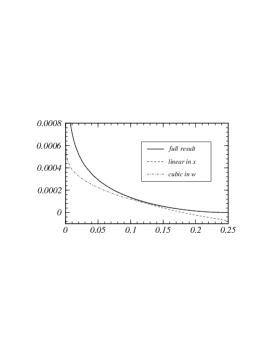
$\displaystyle{\mbox{\hskip 355.65944pt}\bf\frac{m_{1}^{2}}{s}}$

Figure 2: Production rate $R_{f_{1}\bar{f}_{1}f_{2}\bar{f}_{2}}$ based on the exact result (solid line) and approximations described in the text as functions of $m_{1}^{2}/s$ with $m_{1}=m_{\tau}$ and $m_{2}=m_{e}$.

3. Virtual corrections
Virtual corrections in the present context arise from the two particle cut of the “double bubble” diagrams (Fig. 1). The ${\cal O}(\alpha^{2})$ corrections $\delta\Lambda_{\mu}$ to the lowest order vertex can be classified into contributions to the Dirac ($F_{1}$) and the Pauli form factor ($F_{2}$)

$$\delta\Lambda_{\mu}=\gamma_{\mu}\,\left(\frac{\alpha}{\pi}\right)^{2}\,F_{1}+\frac{i}{2\,m_{1}}\,\sigma_{\mu\nu}\,q^{\nu}\,\left(\frac{\alpha}{\pi}\right)^{2}\,F_{2}$$ (12)

where $\sigma_{\mu\nu}=\frac{i}{2}[\gamma_{\mu},\gamma_{\nu}]$ and $q$ denotes the photon momentum flowing into the vertex. Using the dispersive methods applied already in [10, 11] the calculation of $F_{1,2}$ can be easily reduced to a one dimensional integration. It results from the convolution of the massive vector boson exchange vertex correction to $f_{1}\bar{f}_{1}$ production with the absorptive part of the vacuum polarization of fermions with mass $m_{2}$. Denoting the vector boson mass by $\lambda$ the convolution reads

$$F_{1,2} = \frac{1}{3}\,\int_{4\,m_{2}^{2}}^{\infty}\frac{{\rm d}\lambda^{2}}{\lambda^{2}}\,\left(1+\frac{2\,m_{2}^{2}}{\lambda^{2}}\right)\,\sqrt{1-\frac{4\,m_{2}^{2}}{\lambda^{2}}}\,\widehat{F}_{1,2}(\lambda^{2})$$ (13)

with

$$\mbox{Re}\,\widehat{F}_{1}(\lambda^{2}) = -\frac{1}{4\,w}\,\bigg{[}1+{w^{2}}+\frac{1-{w^{2}}}{{w^{2}}}\,\frac{\lambda^{2}}{m_{1}^{2}}\,\bigg{(}1+\frac{\left(3-2\,{w^{2}}\right)\,\left(1-{w^{2}}\right)}{8\,{w^{2}}}\,\frac{\lambda^{2}}{m_{1}^{2}}\bigg{)}\,\bigg{]}\,\Psi(p,\frac{\lambda^{2}}{m_{1}^{2}})\,\,$$ (14)

$$\mbox{}+\bigg{[}\frac{-1+2\,{w^{2}}}{2\,{w^{2}}}+\frac{-3+7\,{w^{2}}+2\,{w^{4}}}{8\,{w^{4}}}\,\frac{\lambda^{2}}{m_{1}^{2}}+{3\over{\frac{\lambda^{2}}{m_{1}^{2}}-4}}\,\bigg{]}\,\Phi(\frac{\lambda^{2}}{m_{1}^{2}})\,\,$$

$$\mbox{}+\frac{1}{16\,{w^{4}}}\,\bigg{[}-3+7\,{w^{2}}+2\,{w^{4}}+\frac{{{\left(1-{w^{2}}\right)}^{2}}\,\left(-3+2\,{w^{2}}\right)}{2\,w}\,\ln p\,\bigg{]}\,\frac{\lambda^{4}}{m_{1}^{4}}\,\ln\frac{\lambda^{2}}{m_{1}^{2}}\,\,$$

$$\mbox{}-\frac{1}{2\,{w^{2}}}\,\bigg{[}1+\frac{1-{w^{2}}}{2\,w}\,\ln p\,\bigg{]}\,\frac{\lambda^{2}}{m_{1}^{2}}\,\ln\frac{\lambda^{2}}{m_{1}^{2}}-\bigg{[}\frac{1}{2}+\frac{1+{w^{2}}}{4\,w}\,\ln p\,\bigg{]}\,\ln\frac{\lambda^{2}}{m_{1}^{2}}\,\,$$

$$\mbox{}+\bigg{[}\frac{{{\left(1-{w^{2}}\right)}^{2}}\,\left(-3+2\,{w^{2}}\right)}{64\,{w^{5}}}\,\ln^{2}p\,\bigg{]}\,\frac{\lambda^{4}}{m_{1}^{4}}\,\,$$

$$\mbox{}+\frac{1}{4\,{w^{2}}}\,\bigg{[}-\left(1+2\,{w^{2}}\right)+\frac{1-{w^{2}}}{2\,w}\,\ln p\,\Big{(}-3+2\,{w^{2}}-\ln p\Big{)}\,\bigg{]}\,\frac{\lambda^{2}}{m_{1}^{2}}\,\,$$

$$\mbox{}-\frac{1}{8\,w}\,\ln p\,\bigg{(}2\,(1+2\,{w^{2}})+(1+{w^{2}})\,\ln p\bigg{)}-1\,,$$

$$\mbox{Re}\,\widehat{F}_{2}(\lambda^{2}) = \frac{{{\left(1-{w^{2}}\right)}^{2}}}{4\,{w^{3}}}\,\bigg{[}1+\frac{3\,\left(1-{w^{2}}\right)}{8\,{w^{2}}}\,\frac{\lambda^{2}}{m_{1}^{2}}\,\bigg{]}\,\frac{\lambda^{2}}{m_{1}^{2}}\,\Psi(p,\frac{\lambda^{2}}{m_{1}^{2}})\,\,$$ (15)

$$\mbox{}+\frac{1-{w^{2}}}{2\,{w^{2}}}\,\bigg{[}1+\frac{3-5\,{w^{2}}}{4\,{w^{2}}}\,\frac{\lambda^{2}}{m_{1}^{2}}\,\bigg{]}\,\Phi(\frac{\lambda^{2}}{m_{1}^{2}})\,\,$$

$$\mbox{}+\frac{{{\left(1+w\right)}^{2}}\,\left(1-{w^{2}}\right)}{16\,{w^{4}}}\,\bigg{[}\frac{3-5\,{w^{2}}}{{{\left(1+w\right)}^{2}}}+\frac{3\,{{\left(1-w\right)}^{2}}}{2\,w}\,\ln p\,\bigg{]}\,\frac{\lambda^{4}}{m_{1}^{4}}\,\ln\frac{\lambda^{2}}{m_{1}^{2}}\,\,$$

$$\mbox{}+\frac{1-{w^{2}}}{2\,{w^{2}}}\,\bigg{[}1+\frac{1-{w^{2}}}{2\,w}\,\ln p\,\bigg{]}\,\frac{\lambda^{2}}{m_{1}^{2}}\,\ln\frac{\lambda^{2}}{m_{1}^{2}}+\bigg{[}\frac{3\,{{\left(1-{w^{2}}\right)}^{3}}}{64\,{w^{5}}}\,{{\ln p}^{2}}\,\bigg{]}\,\frac{\lambda^{4}}{m_{1}^{4}}\,\,$$

$$\mbox{}+\frac{1-{w^{2}}}{4\,{w^{2}}}\,\bigg{[}1+\frac{1-{w^{2}}}{2\,w}\,\ln p\,\Big{(}3+\ln p\Big{)}\,\bigg{]}\,\frac{\lambda^{2}}{m_{1}^{2}}+\frac{1-{w^{2}}}{4\,w}\,\ln p$$

where

$$\Phi(\xi) = \frac{1}{2}\sqrt{\xi^{2}-4\,\xi}\ln\left(\frac{\xi-\sqrt{\xi^{2}-4\,\xi}}{\xi+\sqrt{\xi^{2}-4\,\xi}}\right)\,,$$ (16)

$$\Psi(p,\xi) = \frac{1}{2}\ln^{2}\left(\frac{1}{2}\left[\xi-2+\sqrt{\xi^{2}-4\,\xi}\right]\right)$$ (20)

$$+\mbox{Li}_{2}\left(1+\frac{p}{2}\left[-2+\xi+\sqrt{\xi^{2}-4\,\xi}\right]\right)+\mbox{Li}_{2}\left(1+\frac{p}{2}\left[-2+\xi-\sqrt{\xi^{2}-4\,\xi}\right]\right)$$

$$+\left\{\begin{array}[]{ll}\displaystyle{-\frac{3}{2}\,\pi^{2}+4\,\pi\arctan\left(\frac{\sqrt{4\,\xi-\xi^{2}}}{\xi}\right)+2\,\pi\arctan\left(\frac{2\,p+\xi-2}{\sqrt{4\,\xi-\xi^{2}}}\right)\,,}&0<\xi<4\\ \displaystyle{-\frac{1}{2}\,\pi^{2}+i\,\pi\,\ln\Big{(}(1-p)^{2}+p\,\xi\Big{)}\,,}&\xi>4\end{array}\right.\,.$$

The QED normalization $\widehat{F}_{1}(0)=0$ is evidently adopted. The evaluation of eq. (13) is tedious for arbitrary $m_{1}$ and $m_{2}$ and will be presented in detail in [8]. In the limiting case $m_{1}\gg m_{2}$, however, the result is drastically simplified:

$$\mbox{Re}\,F_{1} = f_{1}^{(2)}\,\ln^{2}\frac{{m_{2}^{2}}}{s}+f_{1}^{(1)}\,\ln\frac{{m_{2}^{2}}}{s}+f_{1}^{(0)}\,,$$ (21)

$$\mbox{Re}\,F_{2} = f_{2}^{(1)}\,\ln\frac{{m_{2}^{2}}}{s}+f_{2}^{(0)}\,$$ (22)

where

$$f_{1}^{(2)} = \mbox{}\frac{1}{12}\,\bigg{[}\,\frac{1+{w^{2}}}{2\,w}\,\ln p+1\,\bigg{]}\,,$$ (23)

$$f_{1}^{(1)} = \mbox{}\frac{1+{w^{2}}}{6\,w}\,\bigg{[}\mbox{Li}_{2}(1-p)+\ln p\,\Big{(}\ln(1+p)-\frac{1}{4}\,\ln p\Big{)}-3\,\zeta(2)\bigg{]}\,\,$$ (24)

$$\mbox{}+\frac{8-6\,w+11\,{w^{2}}}{36\,w}\,\ln p+\frac{1}{3}\,\ln(1+p)+\frac{11}{18}\,,$$

$$f_{1}^{(0)} = \mbox{}\frac{1+{w^{2}}}{3\,w}\,\bigg{[}\,-\mbox{T}_{3}(1,0,w)+\mbox{T}_{3}(1,{1\over w},w)-\mbox{T}_{3}(1,w,{1\over w})+2\,\ln w\,\mbox{T}_{2}(1,w)-\frac{\pi}{2}\,\mbox{T}^{*}_{2}(1,{1\over w})-G\,\pi\,\,$$ (25)

$$\mbox{}\,\quad+\mbox{Li}_{3}({{1-p}\over 2})-\mbox{Li}_{3}(1-p)-\mbox{Li}_{3}({{-1+p}\over{2\,p}})-\frac{1}{2}\,\mbox{Li}_{3}(p)+\frac{1}{2}\,\zeta(3)\,\,$$

$$\mbox{}\,\quad+\frac{1}{2}\,\Big{(}\mbox{Li}_{2}(p)\,\ln({{{w^{4}}\,\left(1-{w^{2}}\right)}\over 4})-\mbox{Li}_{2}({p^{2}})\,\ln w\Big{)}+\frac{1}{2}\,\ln 2\,\ln p\,\ln({{2\,p}\over{{{\left(1-p\right)}^{2}}}})\,\,$$

$$\mbox{}\,\quad+\frac{1}{2}\,\ln p\,\ln^{2}w-\frac{1}{4}\,\ln^{2}p\,\ln(1-{p^{2}})+\frac{5}{24}\,\ln^{3}p+\Big{(}\frac{3}{2}\,\ln(4\,p)-2\,\ln(1+p)\Big{)}\,\zeta(2)\,\bigg{]}\,\,$$

$$\mbox{}-\frac{8+11\,{w^{2}}}{18\,w}\,\bigg{[}\,\mbox{Li}_{2}(p)+\frac{1}{4}\,{{\ln p}^{2}}+\ln p\,\ln w+2\,\zeta(2)\,\bigg{]}\,\,$$

$$\mbox{}+\frac{1}{12}\,\ln^{2}({{1-{w^{2}}}\over 4})+\frac{131-132\,w+134\,{w^{2}}}{216\,w}\,\ln p+\frac{11}{9}\,\ln(1+p)+\frac{1}{3}\,\zeta(2)+\frac{67}{54}\,,$$

$$f_{2}^{(1)} = -\,\frac{1-{w^{2}}}{12\,w}\,\ln p\,,$$ (26)

$$f_{2}^{(0)} = \frac{1-{w^{2}}}{6\,w}\,\bigg{[}\,-\mbox{Li}_{2}(1-p)+\frac{1}{4}\,\ln^{2}p-\ln p\,\ln(1+p)-\frac{25}{12}\,\ln p+3\,\zeta(2)\,\bigg{]}\,$$ (27)

and

$$\mbox{T}_{2}(\eta,\xi) \equiv \int_{0}^{1}{\rm d}x\,\frac{\arctan(\xi\,x)}{x^{2}+\eta^{2}}\,,$$

$$\mbox{T}_{2}^{*}(\eta,\xi) \equiv \int_{0}^{1}{\rm d}x\,\frac{\ln(x^{2}+\xi^{2})}{x^{2}+\eta^{2}}\,,$$

$$\mbox{T}_{3}(\eta,\xi,\chi) \equiv \int_{0}^{1}{\rm d}x\,\frac{\ln(x^{2}+\xi^{2})\,\arctan(\chi\,x)}{x^{2}+\eta^{2}}\,,$$ (28)

$$G = \int_{0}^{1}{\rm d}x\,\frac{\arctan(x)}{x}\,=\,0.915965594177219\ldots\quad\mbox{(Catalan's constant).}$$

Again the functions $f_{1}^{(1,2)}$ and $f_{2}^{(1)}$ are closely related to the very well-known logarithmically divergent and constant pieces of the corresponding one loop corrections for small $\lambda$ [2]:

$$\mbox{Re}\,\widehat{F}_{1} \stackrel{{\scriptstyle\lambda\to 0}}{{\longrightarrow}} \mbox{}6\,\bigg{[}\,f_{1}^{(2)}\,\bigg{(}\ln\frac{s}{\lambda^{2}}+\frac{5}{3}\,\bigg{)}-\frac{1}{2}\,f_{1}^{(1)}\,\bigg{]}\,,$$

$$\mbox{Re}\,\widehat{F}_{2} \stackrel{{\scriptstyle\lambda\to 0}}{{\longrightarrow}} \mbox{}-3\,f_{2}^{(1)}\,.$$ (29)

The similarity of these relations with eq. (4) is evident. Interesting special cases are again the behaviour close to threshold and for high energies. Let us discuss the former:

$$\mbox{Re}\,F_{1} \stackrel{{\scriptstyle w\to 0}}{{\longrightarrow}} \frac{1}{6\,w}\,\bigg{[}\,-3\,\ln\frac{m_{2}^{2}}{s}+6\,\ln w-8\,\bigg{]}\,\zeta(2)+\bigg{[}\,\frac{1}{2}\,\ln\frac{m_{2}^{2}}{s}+\ln 2+\frac{1}{4}\,\bigg{]}\,\,$$ (30)

$$\mbox{}+\frac{1}{6}\,\bigg{[}\,-3\,\ln\frac{m_{2}^{2}}{s}+6\,\ln w-11\,\bigg{]}\,\zeta(2)\,w\,+{\cal O}(w^{2})\,,$$

$$\mbox{Re}\,F_{2} \stackrel{{\scriptstyle w\to 0}}{{\longrightarrow}} \frac{1}{2\,w}\,\zeta(2)+\frac{1}{3}\,\bigg{[}\,\frac{1}{2}\,\ln\frac{m_{2}^{2}}{s}+\ln 2+\frac{13}{12}\,\bigg{]}-\frac{1}{2}\,\zeta(2)\,w\,+{\cal O}(w^{2})\,.$$ (31)

The Coulombic behaviour $\sim 1/w$ is evident from this result. For $F_{1}$ the Coulomb singularity is modified by the logarithmic factor $\ln(m_{2}^{2}/s)$ which is responsible for the ”running” of the coupling constant in the ${\cal O}(\alpha)$ result. It is instructive to combine the vertex correction of ${\cal O}(\alpha)$ and ${\cal O}(\alpha^{2})$ in the region close to threshold. As an illustrative example we will examine the Dirac formfactor for this case. The infrared divergent part of $\widehat{F}_{1}$ vanishes for $w\rightarrow 0$ and therefore

$$\bigg{(}\frac{\alpha}{\pi}\bigg{)}\,\mbox{Re}\,\widehat{F}_{1}+\bigg{(}\frac{\alpha}{\pi}\bigg{)}^{2}\,\mbox{Re}\,F_{1}\quad\stackrel{{\scriptstyle w\to 0}}{{\longrightarrow}}$$ (32)

$$\mbox{}\,\frac{3}{2}\,\frac{\zeta(2)}{w}\,\bigg{(}\frac{\alpha}{\pi}\bigg{)}\,\bigg{[}\,1+\bigg{(}\frac{\alpha}{\pi}\bigg{)}\frac{1}{3}\,\bigg{(}-\ln\frac{m_{2}^{2}}{s\,w^{2}}-\frac{8}{3}\,\bigg{)}\,\bigg{]}$$

$$\mbox{\hskip 11.38109pt}+\frac{3}{2}\,\bigg{(}\frac{\alpha}{\pi}\bigg{)}\,\bigg{[}-1+\bigg{(}\frac{\alpha}{\pi}\bigg{)}\frac{1}{3}\,\bigg{(}\ln\frac{4\,m_{2}^{2}}{s}+\frac{1}{2}\,\bigg{)}\,\bigg{]}\,+{\cal O}(w)\,.$$

The fine structure constant $\alpha$, defined at vanishing momentum transfer, is related to the $\overline{\mbox{MS}}$ coupling constant at subtraction point $\mu^{2}$ by

$$\alpha=\alpha_{\overline{\mbox{\tiny MS}}}(\mu^{2})\bigg{(}1+\frac{\alpha_{\overline{\mbox{\tiny MS}}}(\mu^{2})}{\pi}\,\frac{1}{3}\,\ln\frac{m_{2}^{2}}{\mu^{2}}\,\bigg{)}+{\cal O}(\alpha^{3}_{\overline{\mbox{\tiny MS}}})\,.$$ (33)

At this point it becomes obvious that the natural scale for $\alpha_{\overline{\tiny\mbox{MS}}}$ in the threshold region is given by the nonrelativistic momentum $\mu^{2}=s\,w^{2}$ as far as the $1/w$ terms are concerned. [This holds true as long as $w\,{\scriptscriptstyle\stackrel{{\scriptstyle\scriptscriptstyle>}}{{\sim}}}\,\alpha$. Below this value the approximations used in this work are no longer applicable.] For the correction resulting from transverse photon exchange, which are not enhanced by $1/w$, the scale $\mu^{2}=s/4$ is appropriate. This suggests the following form of the Dirac formfactor in the threshold region

$$\bigg{(}\frac{\alpha}{\pi}\bigg{)}\,\mbox{Re}\,\widehat{F}_{1}+\bigg{(}\frac{\alpha}{\pi}\bigg{)}^{2}\,\mbox{Re}\,F_{1}\quad\stackrel{{\scriptstyle w\to 0}}{{\longrightarrow}}$$ (34)

$$\mbox{}\frac{3}{2}\,\frac{\zeta(2)}{w}\,\bigg{(}\frac{\alpha_{\overline{\tiny\mbox{MS}}}(s\,w^{2})}{\pi}\bigg{)}\bigg{[}\,1-\bigg{(}\frac{\alpha}{\pi}\bigg{)}\frac{8}{9}\,\bigg{]}$$

$$\hskip 8.53581pt\mbox{}\,-\frac{3}{2}\,\bigg{(}\frac{\alpha_{\overline{\tiny\mbox{MS}}}(s/4)}{\pi}\bigg{)}\,\bigg{[}\,1-\bigg{(}\frac{\alpha}{\pi}\bigg{)}\frac{1}{6}\,\bigg{]}\,+\,{\cal O}(w)$$

where the scale in the ${\cal O}(\alpha^{2})$ term is not yet determined. It is clear that the virtual corrections will dominate the rate close to the threshold.

For high energies, on the other hand, one finds

$$\mbox{Re}\,F_{1} \stackrel{{\scriptstyle\frac{m_{1}^{2}}{s}\to 0}}{{\longrightarrow}} \frac{1}{12}\,\ln^{2}\frac{m_{2}^{2}}{s}\,\Big{(}\ln x+1\Big{)}+\frac{1}{12}\,\ln\frac{m_{2}^{2}}{s}\,\bigg{(}-\ln^{2}x+\frac{13}{3}\,\ln x-8\,\zeta(2)+\frac{22}{3}\bigg{)}\,\,$$ (35)

$$\mbox{}+\frac{1}{36}\,\ln^{3}x-\frac{13}{72}\,\ln^{2}x+\bigg{(}\frac{1}{3}\,\zeta(2)+\frac{133}{216}\bigg{)}\,\ln x-\frac{1}{3}\,\zeta(3)-\frac{16}{9}\,\zeta(2)+\frac{67}{54}\,\,$$

$$\mbox{}+x\,\bigg{[}\,\frac{1}{6}\,\ln^{2}\frac{m_{2}^{2}}{s}+\frac{1}{6}\,\ln\frac{m_{2}^{2}}{s}\,\left(\ln x+\frac{13}{3}\right)\,\,$$

$$\mbox{}\,\quad\quad\,-\frac{1}{12}\,\ln^{2}x+\frac{49}{36}\,\ln x-\frac{4}{3}\,\zeta(2)+\frac{115}{108}\,\bigg{]}\,+{\cal O}(x^{2})\,,$$

$$\mbox{Re}\,F_{2} \stackrel{{\scriptstyle\frac{m_{1}^{2}}{s}\to 0}}{{\longrightarrow}} x\,\bigg{[}\,-\,\frac{1}{3}\,\ln\frac{m_{2}^{2}}{s}\,\ln x+\frac{1}{6}\,\ln^{2}x-\frac{25}{18}\,\ln x+\frac{4}{3}\,\zeta(2)\,\bigg{]}\,+{\cal O}(x^{2})\,.$$ (36)

For the special case $m_{1}=m_{2}=m$ the integrals (13) lead to particularly simple results

$$\mbox{Re}\,F_{1} = \frac{1}{12\,{w^{2}}}\,\bigg{[}\,\frac{\left(-1+2\,{w^{2}}\right)\,\left(9-6\,{w^{2}}+5\,{w^{4}}\right)}{24\,{w^{3}}}\,\ln^{3}p+\frac{31-23\,{w^{2}}+30\,{w^{4}}}{12\,{w^{2}}}\,\ln^{2}p\,\,$$ (37)

$$\mbox{}\,\quad+\bigg{(}\frac{267-238\,{w^{2}}+236\,{w^{4}}}{18\,w}+\frac{\left(1-2\,{w^{2}}\right)\,\left(9-6\,{w^{2}}+5\,{w^{4}}\right)}{2\,{w^{3}}}\,\zeta(2)\bigg{)}\,\ln p\,\,$$

$$\mbox{}\,\quad+\frac{9-21\,{w^{2}}-10\,{w^{4}}}{{w^{2}}}\,\zeta(2)+\frac{147+236\,{w^{2}}}{9}\,\bigg{]}\,,$$

$$\mbox{Re}\,F_{2} = \frac{1-{w^{2}}}{4\,{w^{2}}}\,\bigg{[}\,\frac{{{\left(1-{w^{2}}\right)}^{2}}}{8\,{w^{3}}}\,\ln^{3}p-\frac{11-9\,{w^{2}}}{12\,{w^{2}}}\,\ln^{2}p\,\,$$ (38)

$$\mbox{}\,\quad-\Big{(}\frac{93-68\,{w^{2}}}{18\,w}+\frac{3\,{{\left(1-{w^{2}}\right)}^{2}}}{2\,{w^{3}}}\,\zeta(2)\Big{)}\,\ln p-\frac{17}{3}+\frac{-3+5\,{w^{2}}}{{w^{2}}}\,\zeta(2)\,\bigg{]}\,$$

with the high energy expansion

$$\mbox{Re}\,F_{1} \stackrel{{\scriptstyle\frac{m^{2}}{s}\to 0}}{{\longrightarrow}} \frac{1}{36}\,\ln^{3}x+\frac{19}{72}\,\ln^{2}x+\frac{1}{3}\,\Big{(}\frac{265}{72}-\zeta(2)\Big{)}\,\ln x-\frac{11}{6}\,\zeta(2)+\frac{383}{108}\,$$ (39)

$$\mbox{}+x\,\bigg{[}\frac{5}{4}\,\ln^{2}x+\frac{49}{12}\,\ln x-\frac{5}{3}\,\zeta(2)+\frac{853}{108}\bigg{]}\,+{\cal O}(x^{2})\,,$$

$$\mbox{Re}\,F_{2} \stackrel{{\scriptstyle\frac{m^{2}}{s}\to 0}}{{\longrightarrow}} x\,\bigg{[}\,-\frac{1}{6}\,\ln^{2}x-\frac{25}{18}\,\ln x+2\,\zeta(2)-\frac{17}{3}\,\bigg{]}\,+{\cal O}(x^{2})\,.\,$$ (40)

The logarithmically enhanced and the constant parts are in agreement with [12].

Finally, the ${\cal O}(\alpha^{2})$ contribution of the virtual corrections to the rate for the case $m_{1}\gg m_{2}$ is given by

$$\delta R_{V} = \left(\frac{\alpha}{\pi}\right)^{2}\,\varrho^{V}\,,$$

$$\varrho^{V} = w\,(3-w^{2})\,\Big{(}\mbox{Re}\,F_{1}+\mbox{Re}\,F_{2}\Big{)}+w^{3}\,\mbox{Re}\,F_{2}\,.$$ (41)

4. The total rate
Combining real and virtual radiation one thus arrives at

$$\varrho^{R}+\varrho^{V} = -\,\frac{1}{3}\,W\,\ln\frac{m_{2}^{2}}{s}+f_{R}^{(0)}+w\,(3-w^{2})\,\left(f_{1}^{(0)}+f_{2}^{(0)}\right)+w^{3}\,f_{2}^{(0)}\,.$$ (42)

The quadratic logarithm in $m_{2}^{2}/s$ from the real and the virtual radiation cancel. A linear logarithm, however, remains. Its origin can be easily understood through the running of the coupling constant $\alpha$. The prefactor $W$ is identical to the correction function of ${\cal O}(\alpha)$ derived by Schwinger [2]. Therefore the expression for the rate for the inclusive $f_{1}\bar{f}_{1}$ final state including ${\cal O}(\alpha)$ photonic corrections plus photonic ${\cal O}(\alpha^{2})$ corrections due to one light fermion with mass $m_{2}$ reads

$$R = \frac{1}{2}\,w\,(3-w^{2})+\left(\frac{\alpha}{\pi}\right)\,W$$

$$+\left(\frac{\alpha}{\pi}\right)^{2}\,\bigg{[}-\frac{1}{3}\,W\,\ln\frac{m_{2}^{2}}{s}+f_{R}^{(0)}+w\,(3-w^{2})\,\left(f_{1}^{(0)}+f_{2}^{(0)}\right)+w^{3}\,f_{2}^{(0)}\,\bigg{]}$$

where

$$W = -3\bigg{[}f_{R}^{(1)}+w(3-w^{2})\bigg{(}f_{1}^{(1)}+f_{2}^{(1)}\bigg{)}+w^{3}\,f_{2}^{(1)}\bigg{]}=$$ (43)

$$= \mbox{}\frac{\left(3-{w^{2}}\right)\,\left(1+{w^{2}}\right)}{2}\,\bigg{[}\,2\,\mbox{Li}_{2}(p)+\mbox{Li}_{2}({p^{2}})+\ln p\,\Big{(}2\,\ln(1-p)+\ln(1+p)\Big{)}\,\bigg{]}\,\,$$

$$\mbox{}-w\,(3-{w^{2}})\,\Big{(}2\,\ln(1-p)+\ln(1+p)\Big{)}+\frac{\left(-1+w\right)\,\left(33-39\,w-17\,{w^{2}}+7\,{w^{3}}\right)}{16}\,\ln p\,\,$$

$$\mbox{}+\frac{3\,w\,\left(5-3\,{w^{2}}\right)}{8}\,.$$

[Note that the massive quark is not accounted for, consistent with the fact that virtual heavy fermion loops are not considered in eq. (3). Adding virtual corrections eq. (37, 38) and the real radiation, e.g. based on a numerical evaluation of eq. (1) one would thus include “double bubble” diagrams with two massive fermions. This will be done in [8].]

Relating again the fine structure constant $\alpha$ to the $\overline{\mbox{MS}}$ coupling $\alpha_{\overline{\mbox{\tiny MS}}}$ at the scale $\mu^{2}$, the mass singularities disappear and one finds

$$R = \frac{1}{2}\,w\,(3-w^{2})+\bigg{(}\frac{\alpha_{\overline{\tiny\mbox{MS}}}(\mu^{2})}{\pi}\bigg{)}\,W$$ (44)

$$+\,\bigg{(}\frac{\alpha_{\overline{\mbox{\tiny MS}}}(\mu^{2})}{\pi}\bigg{)}^{2}\bigg{[}\,-\frac{1}{3}\,W\,\ln\frac{\mu^{2}}{s}+f_{R}^{(0)}+w\,(3-w^{2})\,\left(f_{1}^{(0)}+f_{2}^{(0)}\right)+w^{3}\,f_{2}^{(0)}\,\bigg{]}\,.$$

The behaviour close to threshold for the choice $\mu^{2}=s$ is easily read off from eq. (44):

$$R \stackrel{{\scriptstyle w\to 0}}{{\longrightarrow}} \frac{3}{2}\,w\,\,$$ (45)

$$\mbox{}+\bigg{(}\frac{\alpha_{\overline{\tiny\mbox{MS}}}(s)}{\pi}\bigg{)}\,\bigg{[}\,\frac{9}{2}\,\zeta(2)-6\,w\,\bigg{]}\,\,$$

$$\mbox{}+{{\bigg{(}\frac{\alpha_{\overline{\tiny\mbox{MS}}}(s)}{\pi}\bigg{)}}^{2}}\,\bigg{[}\,\bigg{(}3\,\ln w-\frac{5}{2}\bigg{)}\,\zeta(2)+\bigg{(}4\,\ln 2+\frac{11}{6}\bigg{)}\,w\,\bigg{]}\,+{\cal O}(w^{2})\,.$$

The discussion following eq. (32) applies equally well to this formula, since real radiation vanishes close to threshold.

In the high energy region one finds

$$R \stackrel{{\scriptstyle\frac{m_{1}^{2}}{s}\to 0}}{{\longrightarrow}} 1-6\,{x^{2}}-8\,{x^{3}}\,\,$$ (46)

$$\mbox{}+\bigg{(}\frac{\alpha_{\overline{\tiny\mbox{MS}}}(s)}{\pi}\bigg{)}\,\bigg{\{}\frac{3}{4}+9\,x+{x^{2}}\,\bigg{[}\,-18\,\ln x+\frac{15}{2}\,\bigg{]}-{x^{3}}\,\bigg{[}\,\frac{116}{3}\,\ln x+\frac{188}{9}\,\bigg{]}\bigg{\}}\,\,$$

$$\mbox{}+{{\bigg{(}\frac{\alpha_{\overline{\tiny\mbox{MS}}}(s)}{\pi}\bigg{)}}^{2}}\,\bigg{\{}\zeta(3)-\frac{11}{8}-\frac{13}{2}\,x\,\,$$

$$\mbox{}\,\qquad+{x^{2}}\,\bigg{[}\,-3\,\ln^{2}x+\frac{27}{2}\,\ln x-4\,\zeta(3)-18\,\zeta(2)-\frac{35}{6}\,\bigg{]}\,\,$$

$$\mbox{}\,\qquad+{x^{3}}\,\bigg{[}\,-8\,\ln^{2}x+\frac{752}{27}\,\ln x-\frac{304}{9}\,\zeta(2)+\frac{1282}{81}\,\bigg{]}\bigg{\}}\,+{\cal O}(x^{4})\,.$$

In Fig. 3 the comparison between the exact ${\cal O}(\alpha^{2})$ correction for $\mu^{2}=s$ (solid line), threshold approximations (dashed dotted lines) and high energy expansions (dashed lines) is performed. Eq. (46) provides an important consistency check on our result. It is straightforward to relate pole and $\overline{\mbox{MS}}$ definition for the remaining fermion mass $m_{1}$ taking again into account in ${\cal O}(\alpha^{2})$ only the contribution from one light virtual fermion:

$$m_{1}^{2} = \overline{m}_{1}^{2}(\mu^{2})\,\bigg{\{}1+\bigg{(}\frac{\alpha_{\overline{\tiny\mbox{MS}}}(\mu^{2})}{\pi}\bigg{)}\,\bigg{[}-\frac{3}{2}\,\ln\frac{\overline{m}_{1}^{2}(\mu^{2})}{\mu^{2}}+2\,\bigg{]}\,\,$$ (47)

$$\mbox{}\qquad\qquad\,\,\,+\bigg{(}\frac{\alpha_{\overline{\tiny\mbox{MS}}}(\mu^{2})}{\pi}\bigg{)}^{2}\,\bigg{[}-\frac{1}{4}\,\ln^{2}\frac{\overline{m}_{1}^{2}(\mu^{2})}{\mu^{2}}+\frac{13}{12}\,\ln\frac{\overline{m}_{1}^{2}(\mu^{2})}{\mu^{2}}-\zeta(2)-\frac{71}{48}\,\bigg{]}\bigg{\}}\,.$$

Replacing the pole mass by the running mass at the scale $\mu^{2}=s$ the logarithmic factor of the $\overline{m}^{2}$ term disappears as expected from general considerations. The structure of the logarithms of the $\overline{m}^{2}$ and $\overline{m}^{4}$ terms coincides with the expectations from [5, 6]. In fact, after replacing the abelian factors by the proper SU(3)-coefficients one obtains

$$R = 1+\bigg{(}\frac{\alpha_{s}(s)}{\pi}\bigg{)}+n_{f}\,\bigg{(}\frac{\alpha_{s}(s)}{\pi}\bigg{)}^{2}\,\bigg{[}\,\frac{2}{3}\,\zeta(3)-\frac{11}{12}\,\bigg{]}\,\,$$ (48)

$$\mbox{}+\frac{\overline{m}_{1}^{2}(s)}{s}\,\bigg{\{}12\,\bigg{(}\frac{\alpha_{s}(s)}{\pi}\bigg{)}-\frac{13}{3}\,n_{f}\,\bigg{(}\frac{\alpha_{s}(s)}{\pi}\bigg{)}^{2}\,\bigg{\}}\,\,$$

$$\mbox{}+\frac{\overline{m}_{1}^{4}(s)}{s^{2}}\,\bigg{\{}-6-22\,\bigg{(}\frac{\alpha_{s}(s)}{\pi}\bigg{)}+n_{f}\,\bigg{(}\frac{\alpha_{s}(s)}{\pi}\bigg{)}^{2}\,\bigg{[}\,\frac{1}{3}\,\ln\frac{\overline{m}_{1}^{2}(s)}{s}-\frac{8}{3}\,\zeta(3)-4\,\zeta(2)+\frac{143}{18}\,\bigg{]}\bigg{\}}\,\,$$

$$\mbox{}+\frac{\overline{m}_{1}^{6}(s)}{s^{3}}\,\bigg{\{}-8+\bigg{(}\frac{\alpha_{s}(s)}{\pi}\bigg{)}\,\bigg{[}\,-\frac{32}{9}\,\ln\frac{\overline{m}_{1}^{2}(s)}{s}-\frac{2480}{27}\,\bigg{]}\,\,$$

$$\mbox{}\,\qquad\qquad+n_{f}\,\bigg{(}\frac{\alpha_{s}(s)}{\pi}\bigg{)}^{2}\,\bigg{[}\,-\frac{4}{3}\,\ln^{2}\frac{\overline{m}_{1}^{2}(s)}{s}+\frac{100}{81}\,\ln\frac{\overline{m}_{1}^{2}(s)}{s}-\frac{176}{27}\,\zeta(2)+\frac{8315}{243}\,\bigg{]}\bigg{\}}$$

where now the number of light fermions, $n_{f}$, is displayed explicitly. The relation to the $n_{f}$ dependent terms of eq. (27) in [6] is evident.

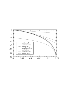
$\displaystyle{\mbox{\hskip 355.65944pt}\bf\frac{m_{1}^{2}}{s}}$

Figure 3: ${\cal O}(\alpha^{2}_{s}(s))$ correction to the inclusive production rate $R_{f_{1}\bar{f}_{1}}$ based on the exact result (solid line) and approximations described in the text.

5. Summary
The rate for the production of a pair of massive fermions in $e^{+}e^{-}$ annihilation plus real and virtual radiation of a pair of light fermions has been calculated analytically. This result, together with [9] can be considered as a first step towards the evaluation of the production cross section for heavy fermions in ${\cal O}(\alpha^{2})$. The expansion of the result for energies close to threshold and for high energies and subsequent comparisons with earlier asymptotic formulas provide important cross checks. The transition to the $\overline{\mbox{MS}}$ scheme leads to interesting insights into the proper scale of the coupling constant.

Acknowledgement: We would like to thank K. Chetyrkin and M. Jeżabek for helpful discussions.

References

References

• [1] V.N. Baĭer, V.S. Fadin and V.A. Khoze, Soviet Physics JETP Lett. 23 (1966) 104.
• [2] J.S. Schwinger, Particles, sources and fields, Addison-Wesley Publishing Company, Inc.(1970/73) and refs. therein.
• [3] K.G. Chetyrkin, A.L. Kataev and F.V. Tkachov, Phys. Lett. B 85 (1979) 277;
M. Dine and J. Sapirstein, Phys. Rev. Lett. 43 (1979) 668;
W. Celmaster and R.J. Gonsalves, Phys. Rev. Lett. 44 (1980) 560.
• [4] S.G. Gorishny, A.L. Kataev and S.A. Larin, Phys. Lett. B 259 (1991) 144;
L.R. Surguladze and M.A. Samuel, Phys. Rev. Lett. 66 (1991) 560 and 2416 (Erratum).
• [5] K.G. Chetyrkin and J.H. Kühn, Phys. Lett. B 248 (1990) 359.
• [6] K.G. Chetyrkin and J.H. Kühn, Nucl. Phys. B 432 (1994) 337.
• [7] L. Lewin, Polylogarithms and associated functions, Elsevier North Holland, Inc., 1981.
• [8] A.H. Hoang, J.H. Kühn and T. Teubner, in preparation.
• [9] A.H. Hoang, M. Jeżabek, J.H. Kühn and T. Teubner, Phys. Lett. B 338 (1994) 330.
• [10] B.A. Kniehl, M. Krawczyk, J.H. Kühn and R.G. Stuart, Phys. Lett. B 209 (1988) 337.
• [11] A.H. Hoang, M. Jeżabek, J.H. Kühn and T. Teubner, Phys. Lett. B 325 (1994) 495 and Phys. Lett. B 327 (1994) 439 (Erratum).
• [12] G.J.H. Burgers, Phys. Lett. B 164 (1985) 167.