The Measurement of Tri-Linear Gauge
Boson Couplings at $e^{+}e^{-}$ Colliders

Abstract

We describe a detailed study of the process $e^{+}e^{-}\to\ell\nu_{\ell}q\bar{q}$ and the measurement of tri-linear gauge boson couplings (TGV’s) at LEP200 and at a 500 GeV and 1 TeV NLC. We included all tree level Feynman diagrams contributing to the four-fermion final states including gauge boson widths and non-resonance contributions. We employed a maximum likelihood analysis of a five dimensional differential cross section of angular distributions. This approach appears to offer an optimal strategy for measurement of TGV’s. LEP200 will improve existing measurements of TGV’s but not enough to see loop contributions of new physics. Measurements at the NLC will be roughly 2 orders of magnitude more precise which would probe the effects of new physics at the loop level.

Introduction

A driving force behind high energy physics is the search for physics beyond the Standard Model (SM). An approach receiving considerable attention generalizes the effects of new physics using effective Lagrangians (${\cal L}_{eff}$) and tests for deviations from SM expectations. While the fermion gauge boson couplings have been measured to high precision by the LEP and SLC experiments the vector boson self-interactions have only just been experimentally verified by direct measurement[1]. Because the standard model makes precise predictions for the TGV’s, precision measurements constitute a stringent test of the gauge structure of the standard model [2]. In this contribution we describe some recent work on precision measurements of tri-linear gauge boson couplings (TGV’s) at $e^{+}e^{-}$ colliders; LEP200 and 500 GeV and 1 TeV versions of the NLC. A more detailed account of this work is given in Ref. [3].

The processes $e^{+}e^{-}\to 4f$, including all tree level Feynman diagrams that contribute to the same final state, have been studied for a number of specific final states; $\ell\nu\ell^{\prime}\bar{\nu}$, $\nu\bar{\nu}\mu^{+}\mu^{-}$, $q\bar{q}q^{\prime}\bar{q}^{\prime}$, and $\ell\nu q\bar{q}$. Our present work consists of a detailed study of the last process, $e^{+}e^{-}\to\ell\nu q\bar{q}$, and its sensitivity to TGV’s. This process can be fully reconstructed and has the advantage of a higher branching ratio than the purely leptonic processes while avoiding the ambiguities and backgrounds associated with the purely hadronic modes.

There are three effective Lagrangians commonly used to describe TGV’s which differ on the degree of generality assumed [2].

1. Most General Parametrization. The only assumptions here are Lorentz and $U(1)_{em}$ invariance. The parameters associated with the CP invariant operators are $g_{1}^{Z}$, $\kappa_{Z}$, $\kappa_{\gamma}$, $\lambda_{Z}$, and $\lambda_{\gamma}$. $g_{\gamma}$ is always equal to 1 and in the SM at tree level $g_{1}^{Z}=\kappa_{V}=1$ and $\lambda_{V}=0$. Typically, radiative corrections from heavy particles will change $\kappa_{V}$ by about 0.015 and $\lambda_{V}$ by about 0.0025. The most robust limits come from associated $W\gamma$ and $WZ$ production at the Tevatron [1]; $-1.6<\delta\kappa_{\gamma}<1.8$, $|\lambda_{\gamma}|<0.6$, $-8.6<\delta\kappa_{Z}<9.0$ and $|\lambda_{Z}|<1.7$.

2. Non-Linearly Realized Goldstone Bosons or The Chiral Lagrangian includes custodial $SU(2)$ symmetry which is experimentally verified to a high degree of accuracy. The parameters of this Lagrangian are $L_{9L}$, $L_{9R}$, and $L_{10}$. $L_{10}$ contributes to the gauge boson self energies where it is tightly constrained to $-1.1\leq L_{10}\leq 1.5$ so we will not consider it further. $L_{9L,9R}$ are expected to be of order 1.

3. Linearly Realized Goldstone Bosons explicitly includes the Goldstone bosons.

Due to space limitations we only present results for the Chiral Lagrangian but note that the different Lagrangians can be mapped onto one another.

Calculations and Results

We studied the final states $\mu^{\pm}\nu_{\mu}q\bar{q}$ and $e^{\pm}\nu_{e}q\bar{q}$. In the first case ten diagrams contribute and in the second, 20 diagrams. We used the CALKUL helicity technique to calculate the amplitudes and integrated the resulting matrix elements using Monte Carlo methods to obtain the cross sections and distributions.

For our numerical results we used the following set of parameters: $\alpha=1/128$, $\sin^{2}\theta_{w}=0.23$, $M_{Z}=91.187$, $\Gamma_{Z}=2.49$, $M_{W}=80.22$ and $\Gamma_{W}=2.08$. We included the kinematic cut $170^{o}>\theta>10^{o}$ where $\theta$ is the angle of the charged lepton, quark, or antiquark relative to the beam axis. We also took $E_{\ell,q,\bar{q}}>10$ GeV. In some of our results we imposed that $|M_{(\ell\nu),(q\bar{q})}-M_{W}|\leq 10$ GeV where $M_{(\ell\nu),(q\bar{q})}$ is the invariant mass of the $\ell\nu\;(q\bar{q})$ pair.

The object of the analysis is to maximize the sensitivity to anomalous gauge boson couplings. The longitudinal components of the $W$ are most sensitive to anomalous couplings. $W^{-}$’s ($W^{+}$’s) produced parallel to the incoming $e^{-}$ ($e^{+}$) are dominated by transverse $W$’s while those in the backward direction have a large $W_{L}$ content. To extract the $W_{L}$’s from the $W_{T}$ “background” we can use the $W$ decay products as a polarimeter; $W_{T}$ decay products peak at forward or backward angles while those of the $W_{L}$’s peak about $\cos\theta=0$ where $\theta$ is the angle of the decay product with respect to the $W$ direction in the $W$ rest frame. The changing mix of $W_{L}$ and $W_{T}$ is illustrated in Fig. 1 by the quark angular distributions for forward and backward $W$ scattering angles $(\Theta)$. Additional information can be obtained by studying the decay product azimuthal distributions which are subject to more complicated interference.

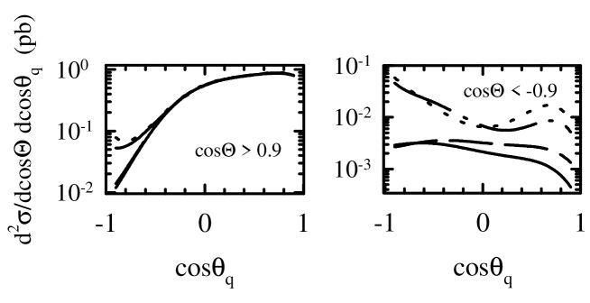
FIG. 1.: Angular distributions of the outgoing quark in the rest frame of the $W^{-}$ in the process $e^{+}e^{-}\to\mu^{+}\nu_{\mu}q\bar{q}$. The solid line is for the SM, the dashed line for $\kappa_{Z}=1.1$, the dotted line for $\lambda_{Z}=0.1$, and the dot-dashed line for $\lambda_{\gamma}=-0.1$.

To determine if anomalous couplings are measurable we use the maximum likelihood method applied to the differential cross section:

$${{d^{5}\sigma}\over{d\cos\Theta d\cos\theta_{q}d\phi_{q}d\cos\theta_{\ell}d\phi_{\ell}}}$$

where $\Theta$ is the scattering angle of the outgoing $W$’s and $\theta_{q(\ell)}$ and $\phi_{q(\ell)}$ are the polar and azimuthal decay angles of the outgoing $q$ ($\ell$) in the $W$ rest frame. We divided each of the angles into 4 bins. Summing over all 1024 bins and comparing the SM predictions to those for anomalous couplings we obtain the log likelihood function:

$${{\ln\cal L}=\sum_{i}[-r_{i}+r_{i}\ln(r_{i})+\mu_{i}-r_{i}\ln(\mu_{i})]}$$

where $r_{i}$ and $\mu_{i}$ are the measured and expected number of events respectively.

We show the 95% C.L. contours for the $L_{9L}-L_{9R}$ plane for LEP200 and 500 GeV and 1 TeV NLC options in Fig. 2.

One can obtain additional information from the processes studied here. Possibilities we have studied but have not included here for lack of space are:

1. Initial state polarization. The distributions are different for left and right handed initial state electrons mainly due to the contributions of the neutrino exchange diagram to the $e^{-}_{L}$ mode but not the $e^{-}_{R}$ mode. This results in different dependences on anomalous couplings adding to the measurement sensitivity.

2. Single $W$ production. In the $e^{+}\nu q\bar{q}$ (or $e^{-}\bar{\nu}q\bar{q}$) final state, instead of imposing the kinematic cut that the final state $e^{+}$ ($e^{-}$) be observed we can impose the cut that it not be observed. In this case the cross section is dominated by the t-channel photon pole providing a mechanism for measuring the $WW\gamma$ vertex independent of the $WWZ$ vertex.

3. Off resonance production. The deviations from the SM value cross sections can be dramatic off the $W$ resonances. Although the off-shell contributions by themselves don’t offer improvements to the on-shell $W$ results, including the off resonance contributions can improve the overall sensitivities in certain cases.

FIG. 2.: 95% confidence level sensitivity contours for $L_{9L}$ and $L_{9R}$ at LEP200 and the 500 GeV and 1 TeV options of the NLC. In all cases the solid lines are the sensitivities obtained by combining the $e^{\pm}$ and $\mu^{\pm}$ modes, the dashed lines are for the $\mu^{+}$ mode only, and the dotted line is for reduced luminosity and combining the 4 modes. (a) $\sqrt{s}=175$ GeV: There are no cuts on $M_{\ell\nu}$ or $M_{q\bar{q}}$. The solid and dashed lines use L=500 pb^-1 and the dotted line uses L=300 pb^-1. (b) 500 GeV: Include the cuts $|M_{\ell\nu(q\bar{q})}-M_{W}|<10$ GeV. The solid and dashed lines use L=50 fb^-1 and the dotted line uses L=10 fb^-1. (c) 1 TeV: Include the cuts $|M_{\ell\nu(q\bar{q})}-M_{W}|<10$ GeV. The solid and dashed lines use L=200 fb^-1. Here the reduced luminosity contour of L=50 fb^-1 lies on top of the $\mu^{+}$ curve.

Summary

We have presented some results from a study of TGV’s in the process $e^{+}e^{-}\to\ell\nu q\bar{q}$. We employed a maximum likelihood analysis of a five dimensional differential cross section of angular distributions. LEP200 will improve on existing measurements, but not sufficiently to observe deviations originating from loop contributions from heavy particles. On the other hand the NLC will be able to measure these couplings to better that a half of a percent which would be sensitive to radiative corrections to the TGV’s.

- [1] H. Aihara, these proceedings; F. Abe et al., Phys. Rev. Lett. 74, 1936 (1995); S. Errede, Proceedings of the 27th International Conference on High Energy Physics, Glasgow, Scotland, July 1994.
- [2] For a recent review see H. Aihara et al., to appear in Electroweak Symmetry Breaking and Beyond the Standard Model, eds. T. Barklow, S. Dawson, H. Haber and J. Siegrist (World Scientific).
- [3] M. Gintner, S. Godfrey, and G. Couture, Carleton report OCIP/C 95-3.