CERN–TH/95–94

hep-ph/9505211

April, 1995

The Higgs Boson Lineshape
 and Perturbative Unitarity

Michael H. Seymour,
Division TH, CERN,
CH-1211 Geneva 23, Switzerland.

Abstract

We discuss the lineshape of a heavy Higgs boson, and the behaviour well above resonance. Previous studies concluded that the energy-dependent Higgs width should be used in the resonance region, but must not be used well away from it. We derive the full result and show that it smoothly extrapolates these limits. It is extremely simple, and would be straightforward to implement in existing calculations.

CERN–TH/95–94
April, 1995

Gauge theories are carefully constructed so as to be well-behaved in the high energy limit. This means not only that they are finite, but that they obey unitarity constraints. This usually comes about by delicate cancelations between different types of contribution, which means that any small changes in the theory, for example anomalous couplings, show up as very large changes in the high energy scattering amplitude.

In the particular case of the electroweak theory, it has long been recognized that high energy scattering of $W$ and $Z$ bosons (which are radiated from incoming quark lines in a hadron-hadron collision) constitutes a crucial test of the theory[1]. Furthermore, if the Higgs boson is heavy, $m_{H}\gg m_{W},$ it will be directly seen as a resonance in the $I\!=\!0$ scattering amplitude. In this case, effective theories have been derived that greatly simplify the calculation of high energy scattering amplitudes[2], since the vector bosons are replaced by the corresponding scalar Goldstone bosons. We use the non-linear $\sigma$-model formulation[3], which has advantages over the usual formulation for our purposes, because the separation into resonant and non-resonant diagrams is the same as in the electroweak theory, allowing a simpler interpretation of the final result. It should be stressed however that we use it purely as a calculational device to reach this result, which is equally valid in the full electroweak theory.

We begin by calculating the amplitude for $W^{+}W^{-}\to ZZ,$ from which all others $VV\to VV$ can be derived by symmetry relations[4], which we give later. The lowest order Feynman diagrams are shown in Fig. 1a, and again in the effective theory in Fig. 1b.

Figure 1: Lowest order Feynman diagrams for $W^{+}W^{-}\to ZZ$ in the electroweak theory (a), and the high-energy effective theory (b), in which the vector bosons are represented by the corresponding Goldstone bosons.

The effective theory correctly reproduces enhanced terms of order $g^{2}m_{H}^{2}/m_{W}^{2}$ and $g^{2}s/m_{W}^{2},$ but not the remainder of the order $g^{2}$ amplitude (we assume $s,m_{H}^{2}\gg m_{W}^{2},$ but make no assumption about their relative size). One gauge cancelation has already taken place, since the last three diagrams of Fig. 1a are separately $\sim s^{2}m_{W}^{4}$ but their sum, the second diagram of Fig. 1b, is $\sim s/m_{W}^{2}$. The result for the amplitude is

$$i{\cal{A}}=\frac{-ig^{2}}{4m_{W}^{2}}\left\{\frac{s^{2}}{s-m_{H}^{2}}-s\right\},$$ (1)

where the two terms correspond to the two diagrams of Fig. 1b. It is clear that at large $s\gg m_{H}^{2},$ another cancelation occurs so that the amplitude remains finite, and satisfies unitarity (except if $m_{H}$ is very large),

$$i{\cal{A}}\;\;{\stackrel{{\scriptstyle s\gg m_{H}^{2}}}{{\longrightarrow}}}\;\;\frac{-ig^{2}m_{H}^{2}}{4m_{W}^{2}},$$ (2)

although the two contributions separately do not.

In the resonance region, $s\sim m_{H}^{2},$ it is clear that the amplitude (1) diverges. As is well known, this is regulated by resumming to all orders the diagrams of Fig. 2. Since each diagram

Figure 2: All orders resummation leading to the Higgs boson self-energy.

contains an additional factor of $1/(s-m_{H}^{2}),$ it is always the leading diagram at that order, and the resummation is justified. The result is[5]

$$i{\cal{A}}\;\;{\stackrel{{\scriptstyle s\sim m_{H}^{2}}}{{\longrightarrow}}}\;\;\frac{-ig^{2}}{4m_{W}^{2}}\frac{s^{2}}{s-m_{H}^{2}+i\mbox{Im}\Pi_{H}(s)},$$ (3)

where $\mbox{Im}\Pi_{H}(s)=m_{H}\Gamma_{H}s^{2}/m_{H}^{4}$ is the imaginary part of the Higgs boson self-energy. Since $\Gamma_{H}/m_{H}\sim g^{2}m_{H}^{2}/m_{W}^{2},$ including the self-energy in the propagator promotes the resonant diagram by one order at the resonance, so one is formally justified in neglecting the non-resonant diagram.

However, inserting (3) into (1), one immediately sees that the high energy behaviour is spoiled, since the resonant diagram is suppressed and the cancelation no longer occurs. The conventional resolution is as follows: Outside the resonance region, the diagrams of Fig. 2 are not enhanced, so there is no justification for resumming them. Therefore the correct result is (3) in the resonance region and (1) outside it.

While this statement is correct theoretically it is not very useful for phenomenology, since one needs an amplitude that smoothly extrapolates the different regions. It is the main aim of this paper to calculate such an amplitude.

Since we have stressed the importance of the cancelation between the resonant and non-resonant diagrams well above resonance, it is natural to wonder whether this cancelation also occurs at each higher order. As we shall show, this is indeed the case, and one can resum a set of diagrams analogous to Fig. 2 but containing both resonant and non-resonant contributions. The result is a smoothly-varying amplitude that agrees, to leading order in $g^{2}\min(m_{H}^{2},s)/m_{W}^{2},$ with (3) in the resonant region, and (1) both above and below it.

We begin by deriving this amplitude for $VV\to VV,$ then show how to generalize it to full electroweak calculations of the process $qq\to qqVV$[6]. As a by-product, we also show how an $s$-channel calculation can be modified to obey unitarity and more closely reproduce the full result. We also discuss the $gg\to VV$ channel and show that the same result applies there. Finally we show numerical results and make some concluding remarks.

For $s\sim m_{H}^{2},$ the amplitudes to scatter $W^{+}W^{-}$ or $ZZ$ to $W^{+}W^{-}$ or $ZZ$ are all equal to the $W^{+}W^{-}\to ZZ$ amplitude,

$$i{\cal{A}}=\frac{-ig^{2}m_{H}^{2}}{4m_{W}^{2}}\frac{s}{s-m_{H}^{2}},$$

where we have included the resonant and non-resonant contributions without keeping track of which is which. The full amplitude for $W^{+}W^{-}\to ZZ$ is then given by a resummation analogous to Fig. 2, but with both resonant and non-resonant graphs appearing in each cell, as shown in Fig. 3. The result is then

Figure 3: All orders resummation leading to the vector boson pair self-energy. Note that both resonant and non-resonant diagrams are included.

$$i\bar{{\cal{A}}}=\sum_{n=0}^{\infty}\left(\frac{3}{2}\frac{1}{16\pi}\int_{-s}^{0}\frac{dt}{s}i{\cal{A}}\right)^{n}i{\cal{A}},$$

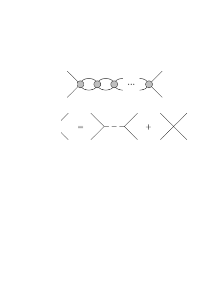
where the integral is the momentum flowing around each loop, and the factor $\frac{3}{2}$ comes from the sum of $WW$ and $ZZ$ in each loop with a factor of $\frac{1}{2}$ for $ZZ$ because they are identical. Using the expression for the Higgs boson width,

$$\Gamma_{H}=\frac{3}{2}\frac{1}{16\pi}\frac{g^{2}m_{H}^{3}}{4m_{W}^{2}},$$

we obtain

$$i\bar{{\cal{A}}} = \sum_{n=0}^{\infty}\left(-i\frac{\Gamma_{H}}{m_{H}}\frac{s}{s-m_{H}^{2}}\right)^{n}\left(\frac{-ig^{2}m_{H}^{2}}{4m_{W}^{2}}\frac{s}{s-m_{H}^{2}}\right)$$

$$= \frac{-ig^{2}m_{H}^{2}}{4m_{W}^{2}}\frac{s}{s-m_{H}^{2}+i\Gamma_{H}s/m_{H}}$$

$$\equiv \frac{-ig^{2}m_{H}^{2}}{4m_{W}^{2}}\frac{s}{s-m_{H}^{2}+i\mbox{Im}\Pi_{VV}(s)},$$

where we dub the function $\Pi_{VV}(s)$ the vector boson pair self-energy. Since we have

$$\mbox{Im}\Pi_{VV}(s)=\frac{m_{H}^{2}}{s}\mbox{Im}\Pi_{H}(s)$$

it is clear that $\mbox{Im}\Pi_{VV}(m_{H}^{2})=\mbox{Im}\Pi_{H}(m_{H}^{2}),$ and (Abstract) is identical to (3) on the resonance.

Equation (Abstract) is the central result of this paper. For $s\gg m_{H}^{2},$ it becomes

$$i\bar{{\cal{A}}}\;\;{\stackrel{{\scriptstyle s\gg m_{H}^{2}}}{{\longrightarrow}}}\;\;\frac{-ig^{2}m_{H}^{2}}{4m_{W}^{2}}\frac{1}{1+i\frac{3}{2}\frac{1}{16\pi}\frac{g^{2}m_{H}^{2}}{4m_{W}^{2}}}=\frac{-ig^{2}m_{H}^{2}}{4m_{W}^{2}}\left(1+{\cal{O}}\left(\frac{g^{2}m_{H}^{2}}{m_{W}^{2}}\right)\right),$$

and for $s\ll m_{H}^{2},$ it becomes

$$i\bar{{\cal{A}}}\;\;{\stackrel{{\scriptstyle s\ll m_{H}^{2}}}{{\longrightarrow}}}\;\;\frac{-ig^{2}s}{4m_{W}^{2}}\frac{1}{-1+i\frac{3}{2}\frac{1}{16\pi}\frac{g^{2}s}{4m_{W}^{2}}}=\frac{ig^{2}s}{4m_{W}^{2}}\left(1+{\cal{O}}\left(\frac{g^{2}s}{m_{W}^{2}}\right)\right).$$

Thus (Abstract) agrees with (1) to leading order in $g^{2}\min(m_{H}^{2},s)/m_{W}^{2}$ above and below the resonance, and (3) on it, smoothly extrapolating the three regions. We therefore describe it as the full leading order amplitude for $W^{+}W^{-}\to ZZ$.

The amplitudes for other scattering processes $VV\to VV$ can be read off from the SO(3) symmetry of the effective theory[Abstract],

$${\cal{A}}(W^{+}W^{-}\to ZZ) \equiv {\cal{A}}(s,t,u),$$

$${\cal{A}}(ZZ\to W^{+}W^{-}) = {\cal{A}}(s,t,u),$$

$${\cal{A}}(W^{+}W^{-}\to W^{+}W^{-}) = {\cal{A}}(s,t,u)+{\cal{A}}(t,s,u),$$

$${\cal{A}}(ZZ\to ZZ) = {\cal{A}}(s,t,u)+{\cal{A}}(t,s,u)+{\cal{A}}(u,t,s),$$

$${\cal{A}}(W^{\pm}W^{\pm}\to W^{\pm}W^{\pm}) = {\cal{A}}(t,s,u)+{\cal{A}}(u,t,s),$$

$${\cal{A}}(W^{\pm}Z\to W^{\pm}Z) = {\cal{A}}(t,s,u).$$

It is important to realize however, that

$$\mbox{Im}\Pi_{VV}(s)=0,\quad s<0,$$

since a space-like pair cannot appear as on-shell lines in a bubble.

To translate (Abstract) to the full electroweak theory, we rewrite it

$$\frac{s}{s-m_{H}^{2}+i\Gamma_{H}s/m_{H}}=\frac{s^{2}/m_{H}(1+i\Gamma_{H}/m_{H})}{s-m_{H}^{2}+i\Gamma_{H}s/m_{H}}-\frac{s}{m_{H}^{2}}.$$ (5)

The apparently higher order term in the numerator is essential for the high energy limit, and cannot be neglected. Equation (5) provides a calculational implementation of (Abstract) that is equally valid in the full electroweak theory. Namely that one makes the replacement

$$\frac{i}{s-m_{H}^{2}}\to\frac{i(1+i\Gamma_{H}/m_{H})}{s-m_{H}^{2}+i\Gamma_{H}s/m_{H}}$$

for the $s$-channel Higgs boson propagator, leaving all other amplitudes unchanged. It would be extremely simple to make this substitution in computer programs that calculate the amplitude for $qq\to qqVV$ such as [6] and, with slightly more effort, in those that directly calculate the differential cross-section.

Unitarity requires that each partial wave of definite angular momentum and isospin, $a^{I}_{J},$ obeys

$$|a^{I}_{J}|\leq 1.$$

Since the condition applies to the exact amplitude, one expects small violations at any given order in perturbation theory, owing to the truncation of the series. However, gross violations should be taken as an indication of the failure of the perturbation series. The $I\!=\!0$ case is obtained by scattering the state $(2W^{+}W^{-}+ZZ)/\surd 6$ to itself, and $J\!=\!0$ from the integral

$$a^{I}_{0}=\frac{1}{16\pi}\int_{-s}^{0}\frac{dt}{s}{\cal{A}}_{I}.$$

For $a^{0}_{0},$ the only partial wave to which the Higgs resonance contributes, we obtain

$$a^{0}_{0}=-\frac{\Gamma_{H}}{m_{H}}\frac{s}{s-m_{H}^{2}+i\Gamma_{H}s/m_{H}}-\frac{2}{3}\frac{\Gamma_{H}}{m_{H}}\left(1-\frac{m_{H}^{2}}{s}\log\left(1+\frac{s}{m_{H}^{2}}\right)\right).$$

This is shown in Fig. 4, in comparison with various amplitudes

Figure 4: The $I\!=\!0,\;J\!=\!0$ partial wave for elastic vector boson scattering with various treatments of the Higgs boson width: zero width (dotted), fixed width (dashed), using the Higgs boson self-energy (dot-dashed), and the full result using the vector boson pair self-energy (solid).

that have been used in the past. Note that only the full amplitude satisfies unitarity both in the resonance region and well above it. Note also that it peaks very close to $m_{H},$ unlike the other cases.

In the resonance region all the possibilities (except the divergent one) are equally valid at leading order, but show marked differences in the lineshape, indicating the need for a full next-to-leading order calculation. However, since the full amplitude is correct above, below and on the resonance, we expect it to give the most accurate lineshape.

Comparing equations (Abstract) and (5), we see the opportunity to make an improvement to the $s$-channel approximation. The $s$-channel approximation consists of using only the diagrams in which the $s$-channel Higgs boson propagator appears, i.e. it gives us the first term of (5). If we multiply this by $m_{H}^{2}/s$ instead of $(1+i\Gamma_{H}/m_{H}),$ we obtain exactly (Abstract). Thus in the $W^{+}W^{-}\to ZZ$ case, this improved $s$-channel approximation is exact. We show numerical results for the $I\!=\!0$ case in Fig. 5.

Figure 5: As in Fig. 4, using the full result (solid), the naïve $s$-channel approximation (dotted) and the improved $s$-channel approximation (dashed).

We turn now to the gluon fusion process. Although the coupling of gluons to electroweak bosons, which is mediated by quark loops, is rather weak, the high density of gluons within a hadron means that this is a competitive source of vector boson pairs. The lowest order diagrams are shown in Fig. 6. The amplitude is[7]

Figure 6: Lowest order Feynman diagrams for $gg\to ZZ$.

$$i{\cal{B}} = \frac{-ig^{2}g_{s}^{2}}{m_{W}^{2}}\left\{\frac{s^{2}}{s-m_{H}^{2}}-s\right\}I(s),$$

$$I(s) = \frac{1}{2}\frac{m_{q}^{2}}{s}\left[\left(\log\frac{s}{m_{q}^{2}}-i\pi\right)^{2}-4\right].$$

Since this has the identical form to (1), it is clear that exactly the same conclusions will apply: the resonant and non-resonant diagrams can be canceled at high energy in each order; they can be resummed to all orders; the result can be implemented by the replacement

$$\frac{i}{s-m_{H}^{2}}\to\frac{i(1+i\Gamma_{H}/m_{H})}{s-m_{H}^{2}+i\mbox{Im}\Pi_{VV}(s)}.$$

Since gluons and vector bosons couple together so weakly, we neglect the effect of internal gluon lines, so

$$\mbox{Im}\Pi_{VV}(s)=\Gamma_{H}s/m_{H}$$

exactly as before.

We have modified the programs of [6] for $qq\to qqVV$ and [8] for $gg\to VV$ according to this prescription, and the results are shown for the LHC in Fig. 7. It can clearly be seen

Figure 7: The $ZZ$ invariant mass spectrum at the LHC from (a) $qq\to qqZZ$ and (b) $gg\to ZZ$. We set $m_{t}=175$ GeV, $m_{Z}=91.2$ GeV, $\alpha=1/128,$ $\sin^{2}\theta_{w}=0.23,$ $m_{W}=m_{Z}\cos\theta_{w}$ and $\alpha_{s}(m_{Z})=0.120,$ and use the MRS D–^′ parton distribution functions. Curves are as in Fig. 4.

that the differences in lineshape and behaviour well above the resonance persist even in the full electroweak calculations convoluted with parton densities. Owing to the fall of parton densities with increasing energy, the full result no longer peaks at the Higgs mass.

We would also like to compare the full result with our improved $s$-channel approximation. However, since the $s$-channel approximation is only intended to model the Higgs boson ‘signal’, and not the ${\cal{O}}(g^{2})$ ‘background’ we compare it with the full result after subtraction of this background. As usual[9], we define the background to be the full result in the limit $m_{H}\to 0,$ as this gives the lowest rate one could expect. It is clear from (1) that this background is zero in the effective theory. The comparison is shown in Fig. 8, where it can be seen that the improved $s$-channel

Figure 8: The excess of the $ZZ$ invariant mass spectrum over the $m_{H}\to 0$ expectation at the LHC from (a) $qq\to qqZZ$ and (b) $gg\to ZZ$. Curves are as in Fig. 5 and parameters as in Fig. 7.

approximation performs much better than the naïve one.

To conclude, the principal result of this paper is shown in Fig. 3 and Eq. (Abstract). It is that it is possible to resum the sum of resonant and non-resonant diagrams to all orders, and the result smoothly extrapolates the well-known correct behaviour below, above and on the resonance. As a calculational prescription, it is possible to represent the result as a modification of the Higgs boson propagator,

$$\frac{i}{s-m_{H}^{2}}\to\frac{i(1+i\Gamma_{H}/m_{H})}{s-m_{H}^{2}+i\Gamma_{H}s/m_{H}},$$

although it should be stressed that it includes effects that are not strictly associated with the propagation of a Higgs boson, namely the interference with non-resonant diagrams. In calculations that use the $s$-channel approximation, a better modification is

$$\frac{i}{s-m_{H}^{2}}\to\frac{im_{H}^{2}/s}{s-m_{H}^{2}+i\Gamma_{H}s/m_{H}}.$$

We have shown that the impact on the Higgs boson lineshape, and hence on the whole phenomenology of high energy vector boson pair production, is significant.

References

1. See for example, J.F. Gunion et al., The Higgs Hunters’ Guide (Addison Wesley, 1990), and references therein

2. M.S. Chanowitz and M.K. Gaillard, Nucl. Phys. B261 (1985) 379

3. G. Valencia and S.S.D. Willenbrock, Phys. Rev. D42 (1990) 853

4. S. Dawson and S.S.D. Willenbrock, Phys. Rev. D40 (1989) 2880

5. G. Valencia and S.S.D. Willenbrock, Phys. Rev. D46 (1992) 2247

6. U. Baur and E.W.N. Glover, Nucl. Phys. B347 (1990) 12

7. E.W.N. Glover and J.J. van der Bij, Phys. Lett. B219 (1989) 488

8. E.W.N. Glover and J.J. van der Bij, Nucl. Phys. B321 (1989) 561

9. E.W.N. Glover, in Proc. 26^th Rencontre de Moriond, High Energy Hadronic Interactions, ed. J. Tran Thanh Van (Editions Frontières, 1991), p. 161