CTEQ/408

MSUHEP-50319

April, 1995

Effects of QCD Resummation on Distributions of
Leptons from the Decay of Electroweak Vector Bosons

Csaba Balázs ^(a),   Jianwei Qiu ^(b)     and   C.-P. Yuan ^(a)

(a) Department of Physics and Astronomy, Michigan State University

East Lansing, MI 48824, U.S.A.

(b) Department of Physics and Astronomy, Iowa State University

Ames, IA 50011, U.S.A.

We study the distributions of leptons from the decay of electroweak vector bosons produced in hadron collisions. The effects of the initial state multiple soft-gluon emission, using the Collins–Soper resummation formalism, are included. The resummed results are compared with the next-to-leading-order results for the distributions of the transverse momentum, rapidity asymmetry, and azimuthal angle of the decay leptons.

1 Introduction

With the discovery of the top quark [1], the electroweak symmetry breaking mechanism remains one of the major mysteries of particle physics today. Unfortunately, the precision low energy data have told us very little about the scalar sector, i.e. the electroweak symmetry breaking sector, of the Standard Model (SM). From CERN LEP data we learned that the mass $m_{H}$ of the Higgs boson has to be larger than about 60 GeV [2]. However, the precision low energy data do not exclude the possibility for $m_{H}$ to be in the order of 1 TeV. At the moment, one of the largest theoretical errors in analyzing radiative corrections to low energy data comes from the prediction of the fine structure constant $\alpha$ evaluated at the $Z$-boson mass scale, due to the less precise low energy $e^{-}e^{+}\rightarrow{\rm hadrons}$ data [3]. Without further improvement in the determination of $\alpha(M_{Z})$, a more precise way to test the SM is to have a better measurement of $M_{W}$. If $M_{W}$ is measured within 40 MeV and the mass of the top quark within 4 GeV, then $m_{H}$ can be constrained within a couple of hundred GeV [4]. To reach such an accuracy in the measurement of $M_{W}$ at hadron colliders, we have to know the kinematics of the $W^{\pm}$-boson well. Since $W^{+}$ decays into a charged lepton $\ell^{+}$ and a neutrino $\nu_{\ell}$, the kinematics of the $W^{+}$ cannot be accurately known because of the missing momentum carried by $\nu_{\ell}$. It is therefore desirable to have a good prediction on the kinematics of $\ell^{\pm}$ from the decay of $W^{\pm}$.

The well established fact that the transverse momentum $Q_{T}$ distribution of the $W^{\pm}$-boson cannot be described by the next-to-leading-order (NLO) perturbative calculation in low $Q_{T}$ region [5] implies that the transverse momentum $p_{T}^{\ell}$ of the lepton $\ell^{\pm}$ cannot be accurately predicted by the NLO calculation, especially for $p_{T}^{\ell}\sim M_{W}/2$ (mostly with low $Q_{T}$) where the data dominate. We must resum the effects of the initial state multiple soft-gluon emission to predict the distributions of the leptons from the decay of the vector boson $V$ ($=\gamma,\,\,W^{\pm}$ or $Z$) produced in hadron collisions. In this paper, we adopt the Collins–Soper formalism [6], and closely follow the notation used in Ref. [7] to resum the multiple soft-gluon effects to the transverse momentum, rapidity asymmetry, and azimuthal angle distributions of the decay product leptons.

2 The Resummation Formalism

To obtain the resummed results, we use dimensional regularization to regulate the infrared (IR) divergencies, and adopt the canonical-$\gamma_{5}$ prescription to calculate the anti-symmetric part of the matrix element in $n$-dimensional space-time. The infrared-anomalous contribution arising from using the canonical-$\gamma_{5}$ prescription was carefully handled by applying the procedures outlined in Ref. [10] for calculating both the virtual and the real diagrams.

The kinematics of the vector boson $V$ (real or virtual) can be expressed in the terms of its mass $Q$, rapidity $y$, transverse momentum $Q_{T}$, and azimuthal angle $\phi_{V}$, measured in the laboratory frame. The kinematics of the leptons from the decay of the vector boson can be described by the polar angle $\theta$ and the azimuthal angle $\phi$, defined in the Collins-Soper frame [11], which is a special rest frame of the $V$-boson [12]. The four-momentum of the decay product fermion in the lab frame is

$$L^{\mu}={Q\over 2}\left({q^{\mu}\over Q}+\sin{\theta}\cos{\phi}~{}X^{\mu}+\sin{\theta}\sin{\phi}~{}Y^{\mu}+\cos{\theta}~{}Z^{\mu}\right),$$ (1)

where

$$q^{\mu}=(M_{T}\cosh{y},\,Q_{T}\cos{\phi},\,Q_{T}\sin{\phi},\,M_{T}\sinh{y}),$$

$$X^{\mu}=-{Q\over Q_{T}M_{T}}\left(q_{+}n^{\mu}+q_{-}{\bar{n}}^{\mu}-{M_{T}^{2}\over Q^{2}}q^{\mu}\right),$$

$$Z^{\mu}={1\over M_{T}}\left(q_{+}n^{\mu}-q_{-}{\bar{n}}^{\mu}\right),$$

$$Y^{\mu}=\varepsilon^{\mu\nu\alpha\beta}{q_{\nu}\over Q}Z_{\alpha}X_{\beta}.$$ (2)

Here, $q_{\pm}={1\over\sqrt{2}}(q^{0}\pm q^{3})$, $M_{T}=\sqrt{Q^{2}+Q^{2}_{T}}$, $n^{\nu}={1\over\sqrt{2}}(1,0,0,1)$ and ${\bar{n}}^{\nu}={1\over\sqrt{2}}(1,0,0,-1)$.

To obtain the fully differential cross section of the vector boson production and decay for all values of $Q_{T}$, we need the resummation formula [7]:

$$\left({d\sigma(AB\rightarrow V(\rightarrow{l{\bar{l}^{\prime}}})X)\over dQ^{2}\,dy\,dQ^{2}_{T}\,d\phi_{V}\,d\cos{\theta}\,d\phi}\right)_{res}={1\over 96\pi^{2}S}\,{Q^{2}\over(Q^{2}-M_{V}^{2})^{2}+M_{V}^{2}\Gamma_{V}^{2}}$$

$$~{}~{}\times\bigg{\{}{1\over(2\pi)^{2}}\int d^{2}b\,e^{i{\vec{q}_{T}}\cdot{\vec{b}}}\,\sum_{j,k}{\widetilde{W}_{jk}(b_{*},Q,x_{A},x_{B},\theta,\phi)}\,F^{NP}_{jk}(b,Q,x_{A},x_{B})$$

$$~{}~{}~{}~{}+~{}Y(Q_{T},Q,x_{A},x_{B},\theta,\phi)\bigg{\}}.$$ (3)

Here $\widetilde{W}_{jk}$ is

$$\widetilde{W}_{jk}(b,Q,x_{A},x_{B},\theta,\phi)=\exp\left\{-S(b,Q)\right\}\mid V_{jk}\mid^{2}$$

$$~{}\times\left\{\left[\left(C_{ja}\otimes f_{a/A}\right)(x_{A})~{}\left(C_{{\bar{k}}b}\otimes f_{b/B}\right)(x_{B})+\left(C_{{\bar{k}}a}\otimes f_{a/A}\right)(x_{A})~{}\left(C_{jb}\otimes f_{b/B}\right)(x_{B})\right]\right.$$

$$~{}~{}~{}~{}~{}\times(g_{L}^{2}+g_{R}^{2})(f_{L}^{2}+f_{R}^{2})(1+\cos^{2}\theta)$$

$$~{}~{}~{}+\left[\left(C_{ja}\otimes f_{a/A}\right)(x_{A})~{}\left(C_{{\bar{k}}b}\otimes f_{b/B}\right)(x_{B})-\left(C_{{\bar{k}}a}\otimes f_{a/A}\right)(x_{A})~{}\left(C_{jb}\otimes f_{b/B}\right)(x_{B})\right]$$

$$~{}~{}~{}~{}~{}\left.\times(g_{L}^{2}-g_{R}^{2})(f_{L}^{2}-f_{R}^{2})(2\cos\theta)\right\},$$ (4)

where $\otimes$ denotes the convolution and is defined by

$$\left(C_{ja}\otimes f_{a/A}\right)(x_{A})=\int_{x_{A}}^{1}{d\xi_{A}\over\xi_{A}}\,f_{a/A}\left(\xi_{A},\mu\right)~{}C_{ja}\left({x_{A}\over\xi_{A}},b,\mu\right),$$ (5)

and the $V_{jk}$ coefficients are given by

$$V_{jk}=\cases{{\rm Cabibbo-Kobayashi-Maskawa~{}matrix~{}elements}&for $V=W^{\pm}$\cr$$\delta_{jk}$$&for $V=Z^{0},\gamma$}.$$ (6)

In the above expressions $j$ represents quark flavors and $\bar{k}$ stands for anti-quark flavors. The dummy indices $a$ and $b$ are meant to sum over quarks and anti-quarks or gluons. Summation on these double indices is implied.

The Sudakov form factor $S(b,Q)$ is defined as

$$S(b,Q)=\int_{b_{0}^{2}/b^{2}}^{Q^{2}}{d{\bar{\mu}}^{2}\over{\bar{\mu}}^{2}}\left[\ln\left({Q^{2}\over{\bar{\mu}}^{2}}\right)A\big{(}\alpha_{s}({\bar{\mu}})\big{)}+B\big{(}\alpha_{s}({\bar{\mu}})\big{)}\right].$$ (7)

The $A$, $B$ functions and the Wilson coefficients $C_{ja}$, etc., were given in Ref. [7]. After fixing the renormalization constants $C_{1}\equiv b_{0}=2e^{-\gamma_{E}}$ and $C_{2}=1$, one can obtain $A^{(1)}$, $B^{(1)}$, $A^{(2)}$ and $B^{(2)}$ from the Eqs. (3.19) to (3.22) of Ref. [7]. ($\gamma_{E}$ is the Euler constant.) After choosing $\mu$ such that $\mu b\equiv C_{3}=2e^{-\gamma_{E}}$, the Wilson coefficients $C^{(i)}_{ja}$ for the parity-conserving part of the resummed result are greatly simplified from the Eqs. (3.23) to (3.26) of Ref. [7] as

$$C^{(1)}_{jk}=\delta_{jk}\left\{{2\over 3}(1-z)+{1\over 3}(\pi^{2}-8)\,\delta(1-z)\right\}~{}~{}~{}{\rm and}~{}~{}~{}C^{(1)}_{jg}={1\over 2}z(1-z).$$ (8)

Following the procedures given in Ref. [10] for handling the $\gamma_{5}$’s in $n$-dimensional space-time, we find that the same Wilson coefficients $C^{(i)}_{ja}$ also apply to the parity-violating part of the resummed result.

In Eq. (3), the impact parameter $b$ is to be integrated from 0 to $\infty$. However, for $b\geq b_{max}$, which corresponds to an energy scale less than $1/b_{max}$, the QCD coupling $\alpha_{s}$ becomes so large that a perturbative calculation is no longer reliable. Hence, the non-perturbative function $F^{NP}$ is needed in the formalism, and generally has the structure

$$F^{NP}_{jk}(b,Q,Q_{0},x_{A},x_{B})=\exp\left[-\ln\left(Q^{2}\over Q^{2}_{0}\right)h_{1}(b)-h_{j/A}(x_{A},b)-h_{{\bar{k}}/B}(x_{B},b)\right],$$ (9)

where $h_{1}$, $h_{j/A}$ and $h_{{\bar{k}}/B}$ cannot be calculated using perturbation theory, so they must be measured experimentally. Furthermore, $\widetilde{W}$ is evaluated at $b_{*}$, with

$$b_{*}={b\over\sqrt{1+(b/b_{max})^{2}}}$$ (10)

such that $b_{*}$ never exceeds $b_{max}$.

The $Y$-term in Eq. (3) is defined as

$$Y(Q_{T},Q,x_{A},x_{B},\theta,\phi)=\int_{x_{A}}^{1}{d\xi_{A}\over\xi_{A}}\int_{x_{B}}^{1}{d\xi_{B}\over\xi_{B}}\sum_{N=1}^{\infty}\left[{\alpha_{s}(Q)\over\pi}\right]^{N}$$

$$\times f_{a/A}(\xi_{A};Q)\,R_{ab}^{(N)}(Q_{T},Q,z_{A},z_{B},\theta,\phi,Q)\,f_{b/B}(\xi_{B};Q),$$ (11)

in which the functions $R_{ab}^{(N)}$ only contain contributions which are less singular than $Q_{T}^{-2}\times$ (logs or 1) as $Q_{T}\rightarrow 0$. Their explicit expressions for ${\bar{\rm p}{\rm p}}\rightarrow V(\rightarrow l{\bar{l}^{\prime}})X$ are given in the Appendix.

3 Numerical Results

In this paper, we only give our numerical results for ${\bar{\rm p}{\rm p}}\rightarrow W^{+}(\rightarrow\ell^{+}\nu_{\ell})X$ at the Fermilab Tevatron with $\sqrt{S}=1.8\,$TeV. The CTEQ3M parton distribution functions (PDF’s) are used along with the non-perturbative function [13]

$$F^{NP}(b,Q,Q_{0},x_{A},x_{B})={\rm exp}\left\{-g_{1}b^{2}-g_{2}b^{2}\ln\left({Q\over 2Q_{0}}\right)-g_{1}g_{3}b\ln{(100x_{A}x_{B})}\right\},$$ (12)

where $g_{1}=0.11\,{\rm GeV}^{2}$, $g_{2}=0.58\,{\rm GeV}^{2}$, $g_{3}=-1.5\,{\rm GeV}^{-1}$ and $Q_{0}=1.6\,{\rm GeV}$. To consistently compare the distributions of the leptons in NLO and resummed calculations, we have used exactly the same PDF’s, QCD and electroweak parameters, etc., for calculating the NLO results. Furthermore, we have applied the kinematic cuts $p_{T}^{\ell}>25\,$GeV, ${\not{\hbox{\kern-4.0pt$E_{T}$}}}>25\,$GeV, and $Q_{T}<20\,$GeV. These cuts are similar to those applied by the CDF group in the measurement of the asymmetry in the lepton rapidity distribution from $W$-boson decays.

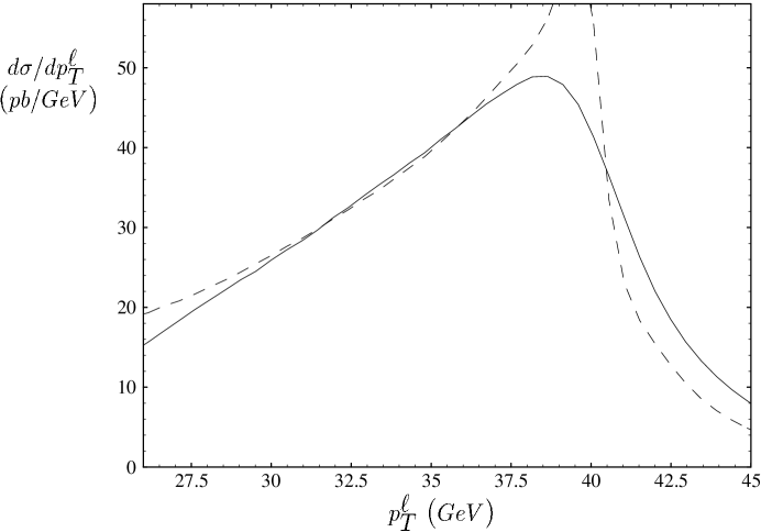
The transverse momentum distributions of the charged lepton $p_{T}^{\ell}$ are shown in Fig. 1 for NLO and resummed calculations. We note that in these results a Breit-Wigner resonant width has been included, cf. Eq. (3). In the vicinity of $p_{T}^{\ell}=M_{W}/2$ (“Jacobian peak”) the NLO calculation is ill-defined because its amplitude blows up as $Q_{T}\rightarrow 0$. The effect of the initial state multiple soft-gluon emission on the distribution of $p_{T}^{\ell}$ is to widen and smoothen the “Jacobian peak” and therefore make it more challenging to accurately extract $M_{W}$ from the $p_{T}^{\ell}$ distribution.

Recently, the Fermilab CDF group measured the asymmetry ${\cal A}_{y^{\ell}}$ in the rapidity $y^{\ell}$ distribution of the charged lepton ($\ell$) from the decay of $W^{+}\rightarrow\ell^{+}\nu_{\ell}$ (or $W^{-}\rightarrow\ell^{-}\bar{\nu}_{\ell}$) [15] and proved this measurement to be particularly sensitive to the slope of the ratio of $u$- to $d$-quark parton densities inside the proton [16, 17].

Figure 1: Transverse momentum distribution of the charged lepton $p_{T}^{\ell}$ for NLO (dashed) and resummed (solid) calculations. Resumming the initial state multiple soft-gluon emission has the typical effect of smoothening and widening the Jacobian peak (at $p_{T}^{\ell}=M_{W}/2$). The NLO distribution is singular and ill-defined near $M_{W}/2$.

FigLCA.eps

Figure 2: The asymmetry ${\cal A}_{y^{\ell}}$ in the lepton rapidity distribution as a function of ${y^{\ell}}$ for NLO (dashed) and resummed (solid) calculations. They differ the most in the large rapidity region ($|y_{\ell^{+}}|>1$). The experimental data were obtained from Ref. [15]

FigDelPhi.eps

Figure 3: The distribution of the difference in the lepton azimuthal angles near the region $\Delta\phi\sim\pi$. The NLO (dashed) distribution is ill-defined at $\Delta\phi=\pi$ and is arbitrary around it. The resummed (solid) distribution gives the correct angular correlation of the lepton pair. The distribution has a similar peak for $\Delta\phi\sim-\pi$.

Define the asymmetry in the lepton rapidity distribution as

$${\cal A}_{y^{\ell}}={{d\sigma/dy^{\ell}}(y^{\ell}>0)-{d\sigma/dy^{\ell}}(y^{\ell}<0)\over{d\sigma/dy^{\ell}}(y^{\ell}>0)+{d\sigma/dy^{\ell}}(y^{\ell}<0)},$$ (13)

which is commonly known as the lepton charge asymmetry. In Fig. 2, we show ${\cal A}_{y^{\ell}}$ as a function of ${y^{\ell}}$ for NLO and resummed calculations. As indicated in the figure, they differ the most in the large rapidity region ($|y_{\ell^{+}}|>1$). Recall that as $Q_{T}\rightarrow 0$ the NLO $Q_{T}$ distribution becomes singular, but the resummed result remains finite. The rapidity $y$ distribution of the $W$-boson in the NLO calculation is not singular, and we expect that after integrating out the complete phase space for $Q_{T}$ (that is, without imposing any kinematic cuts) the NLO and the resummed calculations should predict the same $y$ distributions. We have explicitly checked that this indeed is the case. However, in Fig. 2 some kinematic cuts (as described at the beginning of this section) have been applied to our calculations. In the rest (Collins-Soper) frame of the $W$-boson, the decay kinematics of the lepton $\ell$ is identical for both the NLO and the resummed calculations because the decay leptons do not involve strong interactions. Since the $W$-bosons have different kinematic distributions (e.g., $Q_{T}$ distributions) in these two calculations, the resulting lepton kinematic distributions (e.g., $y^{\ell}$ distributions) in the laboratory frame are different. The two $y^{\ell}$ distributions differ the most in the large $y^{\ell}$ region, where the typical $y$ is large, since the effects of soft-gluon emission become more important, close to the boundary of the phase space.

Another interesting observable to test the QCD theory beyond the fixed-order perturbative calculation is the measurement of the difference in the azimuthal angles of $l$ and ${\bar{l}^{\prime}}$ from the decay of $V$. In practice, this is better measured for $Z\rightarrow\ell^{+}\ell^{-}$. For the sake of argument, we show in Fig. 3 the difference ($\Delta\phi$) in the azimuthal angles of $\ell^{+}$ and $\nu_{\ell}$ measured in the laboratory frame for $W^{+}\rightarrow\ell^{+}\nu_{\ell}$ and calculated in NLO and resummed approaches. As clearly indicated, the NLO result is ill-defined in the vicinity of $\Delta\phi\sim\pm\pi$, where the multiple soft-gluon radiations have to be resummed to obtain physical predictions. Therefore, the transverse mass distributions of $\ell^{+}$-$\nu_{\ell}$ pair for NLO and resummed calculations are also different, and in principle only the resummed results can sensibly predict the distributions of the leptons for a precise measurement of $M_{W}$.

In conclusion, we found that the distributions ($p_{T}^{\ell}$, $y^{\ell}$ and $\Delta\phi$) of leptons are different in NLO and resummed calculations. For a better measurement of $M_{W}$ and $A_{y^{\ell}}$, the effects of the initial state multiple soft-gluon emission have to be considered in hadron collisions. The more detailed phenomenological studies will be presented elsewhere.

Appendix

Let us define the $q\bar{q^{\prime}}V$ and the $l\bar{l^{\prime}}V$ vertices, respectively, as

$$i\gamma_{\mu}\left[g_{L}(1-\gamma_{5})+g_{R}(1+\gamma_{5})\right]~{}~{}~{}{\rm and}~{}~{}~{}i\gamma_{\mu}\left[f_{L}(1-\gamma_{5})+f_{R}(1+\gamma_{5})\right].$$ (14)

For example, for $V=W^{+},q=u$, ${\bar{q}^{\prime}}={\bar{d}}$, $l=\nu_{e}$, and ${\bar{l}^{\prime}}=e^{+}$, the couplings $g_{L}^{2}=f_{L}^{2}=G_{F}M_{W}^{2}/\sqrt{2}$ and $g_{R}^{2}=f_{R}^{2}=0$. ($G_{F}$ is the Fermi constant.) In Eq. (11), for $N=1$,

$$R_{ab}^{(1)}={16\mid V_{jk}\mid^{2}\over\pi Q^{2}}\left[(g_{L}^{2}+g_{R}^{2})(f_{L}^{2}+f_{R}^{2})R_{1}^{ab}+(g_{L}^{2}-g_{R}^{2})(f_{L}^{2}-f_{R}^{2})R_{2}^{ab}\right],$$ (15)

where the coefficient functions $R^{ab}_{i}$ are given as follows:

$$R_{1}^{j{\bar{k}}}=r^{j{\bar{k}}}{\cal L}_{0}+{{\cal R_{+}}(t,u)\over s}\,\delta(s+t+u-Q^{2})\left[{\cal A}_{0}+{\cal A}_{2}+{Q\over Q_{T}}{\cal A}_{1}\right]{Q^{2}\over M_{T}^{2}},$$

$$R_{2}^{j{\bar{k}}}=r^{j{\bar{k}}}{\cal A}_{3}+{{\cal R_{+}}(t,u)\over s}\,\delta(s+t+u-Q^{2})$$

$$~{}~{}~{}~{}~{}~{}~{}~{}~{}~{}~{}~{}\times\left\{{Q^{2}\over Q_{T}^{2}}\left({Q\over M_{T}}-1\right){\cal A}_{3}-{2Q^{2}\over Q_{T}M_{T}}{{\cal R_{-}}(t,u)\over{\cal R_{+}}(t,u)}{\cal A}_{4}\right\},$$ (16)

$$R_{1}^{gj}=r^{gj}{\cal L}_{0}-{Q^{2}Q_{T}^{2}\over uM_{T}^{2}}\,{{\cal R_{+}}(u,s)\over s}\,\delta(s+t+u-Q^{2})$$

$$~{}~{}~{}~{}~{}~{}~{}~{}~{}~{}~{}~{}\times\left\{{{\cal R_{+}}(u,-s)\over{\cal R_{+}}(u,s)}\left[{\cal A}_{0}+{\cal A}_{2}\right]+{Q\over Q_{T}}{(Q^{2}-u)^{2}+{\cal R_{-}}(u,t)\over{\cal R_{+}}(u,s)}{\cal A}_{1}\right\},$$

$$R_{2}^{gj}=r^{gj}{\cal A}_{3}-{Q_{T}^{2}\over u}~{}{{\cal R_{+}}(u,s)\over s}\,\delta(s+t+u-Q^{2})$$

$$~{}~{}~{}~{}~{}~{}~{}~{}~{}~{}~{}~{}\times\left\{{Q^{2}\over Q_{T}^{2}}\left[{Q\over M_{T}}\left({2u(Q^{2}-s)\over{\cal R_{+}}(u,s)}-1\right)-1\right]{\cal A}_{3}\right.$$

$$~{}~{}~{}~{}~{}~{}~{}~{}~{}~{}~{}~{}~{}~{}~{}~{}~{}~{}~{}~{}\left.-{2Q^{2}\over Q_{T}M_{T}}\left[{2s(Q^{2}-s)\over{\cal R_{+}}(u,s)}+1\right]{\cal A}_{4}\right\},$$

with

$$r^{j{\bar{k}}}={Q^{2}\over Q_{T}^{2}}\Bigg{\{}{{\cal R}_{+}(t,u)\over s}~{}\delta(s+t+u-Q^{2})-2~{}\delta(1-z_{A})~{}\delta(1-z_{B})\left[\ln{\left({Q^{2}\over Q_{T}^{2}}\right)}-{3\over 2}\right]$$

$$~{}~{}~{}~{}~{}~{}~{}~{}~{}~{}~{}~{}~{}~{}~{}-\delta(1-z_{A})\left({1+z_{B}^{2}\over 1-z_{B}}\right)_{+}-\delta(1-z_{B})\left({1+z_{A}^{2}\over 1-z_{A}}\right)_{+}\Bigg{\}},$$ (17)

and

$$r^{gj}={Q^{2}\over Q_{T}^{2}}\left\{-{Q_{T}^{2}\over u}~{}{{\cal R_{+}}(u,s)\over s}\,\delta(s+t+u-Q^{2})-\left[z_{A}^{2}+(1-z_{A})^{2}\right]\,\delta(1-z_{B})\right\},$$ (18)

where ${\cal R_{\pm}}(t,u)=(Q^{2}-t)^{2}\pm(Q^{2}-u)^{2}$. The angular dependence is described by the functions

$${\cal L}_{0}=1+\cos^{2}{\theta},~{}{\cal A}_{0}={1\over 2}(1-3\cos^{2}{\theta}),~{}{\cal A}_{1}=\sin{2\theta}\cos{\phi},~{}{\cal A}_{2}={1\over 2}\sin^{2}{\theta}\cos{2\phi},~{}$$

$${\cal A}_{3}=2\cos{\theta},~{}{\cal A}_{4}=\sin{\theta}\cos{\phi},$$ (19)

of which ${\cal A}_{3}$ and ${\cal A}_{4}$ are odd under parity operation.

References

• [1] CDF Collaboration (F. Abe, et al.), Phys. Rev. Lett. 74 (1995) 2626
DØ  Collaboration (S. Abachi, et al.), Phys. Rev. Lett. 74 (1995) 2632.
• [2] Review of Particle Properties, Phys. Rev. D 50 (1994) 1173.
• [3] Morris L. Swartz, SLAC preprint SLAC-PUB-6710, November 1994.
• [4] J. Rosner, report EFI 94-38, August 1994,
• [5] G. Altarelli, R.K. Ellis, M. Greco, G. Martinelli, Nucl. Phys. B 246 (1984) 12.
• [6] J. Collins and D. Soper, Nucl. Phys. B 193 (1981) 381; Erratum B 213 (1983) 545; B 197 (1982) 446.
• [7] J. Collins, D. Soper and G. Sterman, Nucl. Phys. B 250 (1985) 199.
• [8] G. t’Hooft and M. Veltman, Nucl. Phys. B 44 (1972) 189;
P. Breitenlohner and D. Maison, Comm. Math. Phys. 52 (1977) 11.
• [9] J.G. KΓΆrner, G. Schuler, G. Kramer, B. Lampe, Z. Phys. C 32 (1986) 181.
• [10] J.G. KΓΆrner, E. Mirkes, G. Schuler, Internat. J. of Mod. Phys. A Vol. 4, No.7 (1989) 1781.
• [11] J. Collins and D. Soper, Phys. Rev. D 16 (1977) 2219.
• [12] C.S. Lam, Wu-Ki Tung, Phys. Rev. D 18 (1978) 2447.
• [13] G.A. Ladinsky and C.-P. Yuan, Phys. Rev. D 50 (1994) 4239 .
• [14] W. Giele, E.Glover, D.A. Kosover, Nucl. Phys. B 403 (1993) 633.
• [15] M. Dickson, Tests of Structure Functions using Leptons with CDF, in: High-Energy Physics. Proceedings, International Europhysics Conference (Marseille, France, July 22-28, 1993), ed. J. Carr, M. Perrottet (Gif-sur-Yvette, France, 1994)
• [16] E.L. Berger, F. Halzen, C.S. Kim, S. Willenbrock, Phys. Rev. D 40 (1989) 83; erratum, ibid. D 40 (1989) 3789.
• [17] H.L. Lai, J. Botts, J. Huston, J.G. Morfin, J.F. Owens, J.W. Qiu, W.K. Tung, H. Weerts, MSU preprint MSU-HEP-41024, Oct 1994.