The Vector Current Correlator $<0|T(V^{3}_{\mu}V^{8}_{\nu})|0>$
To Two Loops in Chiral Perturbation Theory
ADP-95-27/T181 hep-ph/9504404

Abstract

The isospin-breaking correlator of the product of flavor octet vector currents, $\Pi^{38}_{\mu\nu}(q^{2})$ $=i\int d^{4}x\ \exp(iq.x)\ <0|T(V^{3}_{\mu}(x)V^{8}_{\nu}(0))|0>$, is computed to next-to-next-to-leading (two-loop) order in Chiral Perturbation Theory. Large corrections to both the magnitude and $q^{2}$-dependence of the one-loop result are found, and the reasons for the slow convergence of the chiral series for the correlator given. The two-loop expression involves a single ${\cal O}(q^{6})$ counterterm, present also in the two-loop expressions for $\Pi^{33}_{\mu\nu}(q^{2})$ and $\Pi^{88}_{\mu\nu}(q^{2})$, which counterterm contributes a constant to the scalar correlator $\Pi^{38}(q^{2})$, defined by $\Pi^{38}_{\mu\nu}(q^{2})\equiv(q_{\mu}q_{\nu}-q^{2}g_{\mu\nu})\Pi^{38}(q^{2})$. The feasibility of extracting the value of this counterterm from other sources is discussed. Analysis of the slope of the correlator with respect to $q^{2}$ using QCD sum rules is shown to suggest that, even to two-loop order, the chiral series for the correlator may not yet be well-converged.

I Introduction

In the last decade, following the appearance of the classic papers of Gasser and Leutwyler[2, 3, 4] , numerous treatments of low-energy hadronic properties employing the methods of Chiral Perturbation Theory (ChPT) have appeared (for an excellent recent review, see Ref.[5]). In the bulk of these treatments, the chiral expansion has been carried out to next-to-leading (one-loop) order (i.e. ${\cal O}(q^{4})$ in the usual chiral counting). Expressions for hadronic observables, to this order, incorporate the constraints of current algebra and, in addition, provide the leading corrections to these constraints in a transparent and unambiguous manner. For many processes (see again Ref.[5]) corrections to leading order results are $\simeq 20-30\%$, and truncating the full chiral series to this order, in consequence, appears well-justified. This is, however, not universally the case. For example, the one-loop amplitude for $\gamma\gamma\rightarrow\pi^{0}\pi^{0}$ [6, 7], which vanishes at leading order, differs significantly from experiment even near threshold. The same is true of the spectral function of the vector current correlator $\Pi^{33}_{\mu\nu}(q^{2})$, where

$$\Pi^{ab}_{\mu\nu}(q^{2})=i\int d^{4}x\ \exp(iq.x)\ <0|T(V^{a}_{\mu}(x)V^{b}_{\nu}(0))|0>\equiv(q_{\mu}q_{\nu}-q^{2}g_{\mu\nu})\Pi^{ab}(q^{2})$$ (1)

with $V^{a}_{\mu}$ the standard flavor octet vector current, $V^{a}_{\mu}=\bar{q}{\lambda^{a}\over 2}\gamma_{\mu}q$, again even rather near $\pi\pi$ threshold[8] . Even more dramatic is the case of the process $\eta\rightarrow\pi^{0}\gamma\gamma$, for which the predicted one-loop branching ratio[9, 10] is a factor of $\simeq 170$ smaller than the Particle Data Group [11] value. In the first two cases, the discrepancies between the one-loop results and experiment are a result of the fact that the leading order contributions vanish. Corrections at ${\cal O}(q^{6})$ are not unexpectedly large, and recent calculations to two-loop order, by Bellucci et al.[12] for $\gamma\gamma\rightarrow\pi^{0}\pi^{0}$, and by Golowich and Kambor[8] for the spectral functions of $\Pi^{33}_{\mu\nu}$ and $\Pi^{88}_{\mu\nu}$, demonstrate that inclusion of the ${\cal O}(q^{6})$ corrections to the ${\cal O}(q^{4})$ one-loop results brings the theoretical predictions nicely into accord with experiment for $q^{2}$ less than $\sim(8-9)\,m_{\pi}^{2}$. The importance of two-loop contributions, even rather near threshold, has also been demonstrated for the photon vacuum polarization function in Ref. [13]. The situation for $\eta\rightarrow\pi^{0}\gamma\gamma$ (which most closely resembles the case at hand) will be discussed in more detail below. Other examples of the necessity of including ${\cal O}(q^{6})$ contributions, in the odd intrinsic parity sector of ${\cal L}_{eff}$, are also known, specifically $\pi^{0}\rightarrow\gamma\gamma^{*}$, $\eta\rightarrow\gamma\gamma^{*}$ [14, 15] and $\gamma\pi^{+}\rightarrow\pi^{+}\pi^{0}$, $\eta\rightarrow\gamma\pi^{+}\pi^{-}$[14, 15, 16].

In the present paper we will study the convergence of the isospin-breaking vector current correlator, $\Pi^{38}_{\mu\nu}$, to two-loop order. We will show that, as for the chiral series of the amplitude for $\eta\rightarrow\pi^{0}\gamma\gamma$, that of the correlator, $\Pi^{38}_{\mu\nu}$, is quite poorly converged to one-loop order, and discuss the physical reasons for this similarity. We will also discuss evidence that, even to two-loop order, the latter series is not yet well-converged. It should be stressed that the correlator in question is of interest not only as an example of a quantity for which the chiral series is slowly converging, but is also of relevance to ongoing debates concerning the role of isospin-mixed vector meson exchange in isospin-breaking and, more particularly, charge-symmetry-breaking, observables in few-body systems (see Ref.[17] for a discussion of a number of the contentious issues and list of other relevant references). Here the point is that one may choose the vector currents, rescaled by $g_{V}/m_{V}^{2}$ (where $m_{V}$, $g_{V}$ are the corresponding vector meson masses and decay constants, the latter defined via $<0|V^{a}_{\mu}|V^{a}(\lambda)>\equiv{m_{V}^{2}\over g_{V}}\epsilon^{\lambda}_{\mu}$ with $a$ the flavor and $\lambda$ the polarization label of the vector meson) as interpolating fields for the vector mesons. The isospin-breaking correlators $\Pi^{38}_{\mu\nu}$ and $\Pi^{30}_{\mu\nu}$ then provide information on the $q^{2}$-dependence of the off-diagonal elements of the vector meson propagator matrix, for this choice of interpolating fields. While the off-shell behavior of such propagator matrix elements is, in general, interpolating-field-dependent, one could couple the results for the propagator to those for the corresponding nucleon-vector meson vertices, obtained using the same choice of vector meson interpolating fields, to produce the relevant isospin-breaking contributions to $NN$ scattering S-matrix elements, such S-matrix elements being independent of the choice of interpolating fields[18]. Finally, it should also be pointed out that the spectral function of $\Pi^{38}_{\mu\nu}$ is, at least in principle, measurable experimentally, though the accuracy required to extract it makes this a rather moot point, at present. The possibility of this extraction rests on the observation that the isovector vector current matrix elements $<\pi\pi|V^{k}_{\mu}|0>$ ($k=1,2,3$) receive isospin-breaking contributions only at second order in $(m_{d}-m_{u})$ [19, 20], whereas $<\pi\pi|V^{8}_{\mu}|0>$ is non-zero already at ${\cal O}(m_{d}-m_{u})$. This means that the deviation of the ratio of vector spectral functions measured in $\tau^{-}\rightarrow\nu_{\tau}\pi^{-}\pi^{0}$ and $e^{+}e^{-}\rightarrow\pi^{+}\pi^{-}$ from that predicted by isospin symmetry is (up to corrections for the heavy quark pieces of the electromagnetic (EM) current) a direct measure of the spectral function of $\Pi^{38}_{\mu\nu}$. Since these effects will be seen to be of order a few times $10^{-4}$ they are, however, well outside the reach of current experiments, for which cross-sections below the resonace region in $e^{+}e^{-}\rightarrow\pi^{+}\pi^{-}$ are known typically to an accuracy of only $\simeq 10\%$.

The remainder of the paper is organized as follows. In Section II we record the relevant terms of the effective Lagrangian at orders 2, 4 and 6 in the chiral expansion, and discuss the general, diagrammatic structure of the one-loop and two-loop results. In Section III we describe briefly some details of the calculations and quote the full one- and two-loop results for the contributions identified in Section II. Detailed formulae for the loop integrals entering these expressions are relegated to the Appendix. Since these integrals have been discussed in considerable detail elsewhere (see, for example Refs.[8, 21]), the Appendix will be rather brief, and the reader is referred to the references just cited for further details. Section IV provides a discussion of the results, in particular the physical origin of the slow convergence of the chiral series for the correlator to one-loop. In Section V, a rough estimate of the single ${\cal O}(q^{6})$ counterterm appearing in the ${\cal O}(q^{6})$ corrections to the one-loop result is given, based on a QCD sum rule analysis of the correlator, and the possibility of independent estimates of this low-energy constant from other sources discussed. The issue of the convergence of the chiral series to two-loop order is also treated. Finally, in Section VI, we summarize our conclusions.

II The Chiral Lagrangian to ${\cal O}(q^{6})$ and the Structure of the Contributions to the Correlator

The leading terms in the low-energy, chiral expansion of the correlator, $\Pi^{38}_{\mu\nu}$, may be obtained from the effective chiral Lagrangian, ${\cal L}_{eff}$, which may be written in the form

$${\cal L}_{eff}={\cal L}^{(2)}+{\cal L}^{(4)}+{\cal L}^{(6)}+\cdots$$ (2)

where the superscripts denote the chiral order. The general form of ${\cal L}^{(2)}$ and ${\cal L}^{(4)}$, in the presence of external scalar, pseudoscalar, vector and axial vector sources, is given in Ref.[2] . Since we are interested only in the correlator of vector currents we may set the external pseudoscalar and axial sources to zero and the external scalar source to $2B_{0}\,M$, where $M$ is the current quark mass matrix and $B_{0}$ the usual parameter, appearing in ${\cal L}^{(2)}$ and related to the value of the quark condensate. One then has, explicitly, for ${\cal L}^{(2)}$ and ${\cal L}^{(4)}$[2]

$${\cal L}^{(2)}={1\over 4}f^{2}\text{Tr}(D_{\mu}UD^{\mu}U^{\dagger})+{1\over 2}f^{2}\text{Tr}[B_{0}M(U+U^{\dagger})]$$ (3)

and

$${\cal L}^{(4)} = L_{1}\bigl{[}\text{Tr}(D_{\mu}UD^{\mu}U^{\dagger})\bigr{]}^{2}$$ ()

$$\mbox{}+L_{2}\text{Tr}(D_{\mu}UD_{\nu}U^{\dagger})\text{Tr}(D^{\mu}UD^{\nu}U^{\dagger})+L_{3}\text{Tr}(D_{\mu}U^{\dagger}D^{\mu}UD_{\nu}U^{\dagger}D^{\nu}U)$$

$$\mbox{}+L_{4}\text{Tr}(D_{\mu}UD^{\mu}U^{\dagger})\text{Tr}[2B_{0}M(U+U^{\dagger})]+L_{5}\text{Tr}\bigl{[}2B_{0}(MU+U^{\dagger}M)D_{\mu}U^{\dagger}D^{\mu}U\bigr{]}$$

$$\mbox{}+L_{6}\bigl{[}\text{Tr}[2B_{0}M(U+U^{\dagger})]\bigr{]}^{2}+L_{7}\bigl{[}\text{Tr}[2B_{0}M(U-U^{\dagger})]\bigr{]}^{2}$$

$$\mbox{}+L_{8}\text{Tr}[4B_{0}^{2}(MUMU+MU^{\dagger}MU^{\dagger})]-iL_{9}\text{Tr}[F_{\mu\nu}D^{\mu}UD^{\nu}U^{\dagger}+F_{\mu\nu}D^{\mu}U^{\dagger}D^{\nu}U]$$

$$\mbox{}+L_{10}\text{Tr}[U^{\dagger}F_{\mu\nu}UF^{\mu\nu}]+H_{1}\text{Tr}[F_{\mu\nu}F^{\mu\nu}+F_{\mu\nu}F^{\mu\nu}]+H_{2}\text{Tr}[4B_{0}^{2}M^{2}]~{}.$$

In Eqns. (2.2) and (2.3), $B_{0}$ is a mass scale related to the value of the quark condensate in the chiral limit, $U=\text{exp}(i\vec{\lambda}\cdot\vec{\pi}/f)$ (with $\vec{\lambda}$ the usual $SU(3)$ Gell-Mann matrices and $\vec{\pi}$ the octet of pseudoscalar (pseudo-) Goldstone boson fields), $f$ is a dimensionful constant, equal to $f_{\pi}$ in leading order, $M$ is the current quark mass matrix, and $D_{\mu}$ is the covariant derivative which, in the absence of external axial vector sources, takes the form

$$D_{\mu}U=\partial_{\mu}U-i[v_{\mu},U].$$ (9)

The vector field strength tensor, $F_{\mu\nu}$, occuring in Eqn. (2.3) is defined by $F_{\mu\nu}=\partial_{\mu}v_{\nu}-\partial_{\nu}v_{\mu}-i[v_{\mu},v_{\nu}]$, where $v_{\mu}={\lambda^{a}\over 2}v^{a}_{\mu}$, with $v_{\mu}^{a}$ the octet of external $SU(3)$ vector fields. For the case at hand we require only the external sources $v^{3}_{\mu}$ and $v^{8}_{\nu}$ and hence the last term in $F_{\mu\nu}$ vanishes. Note that one would have to supplement Eqn. (2.3) with additional terms involving $\text{Tr}(F_{\mu\nu})$ if one wished to treat the correlator $\Pi^{30}_{\mu\nu}$ but, as these terms do not enter the calculation of $\Pi^{38}_{\mu\nu}$, we have not explicitly displayed them in (2.4). Note also that, in writing the form (2.3) for ${\cal L}^{(4)}$, additional terms which vanish as a consequence of the lowest order equation of motion have been omitted. In performing calculations to ${\cal O}(q^{6})$ one would, in general, also have to include these terms. However, since the effect of their presence can always be absorbed into a redefinition of the coefficients occuring in ${\cal L}^{(6)}$ [5, 22], we may drop these terms from the outset.

The general form of ${\cal L}^{(6)}$, in the presence of external sources, has been determined recently by Fearing and Scherer[23]. The full expression, however, contains 111 terms of even intrinsic parity and 32 of odd intrinsic parity, and so will not be recorded here. In fact, only one combination of the terms from ${\cal L}^{(6)}$ actually enters the present calculation. It is easy to see why this is the case. As pointed out in Ref.[8], since to ${\cal O}(q^{6})$ only terms from ${\cal L}^{(6)}$ zeroth order in the meson fields contribute to vacuum expectations, and since only four terms of the 143 mentioned above contain terms zeroth order in the meson fields and second order in the external vector sources $v^{3}_{\mu}$ and $v^{8}_{\nu}$, only these four terms can contribute to the correlators $\Pi^{ab}_{\mu\nu}$, with $a,b=3,8$. ${\cal L}^{(6)}$ thus reduces, for the purpose of computing such vacuum correlators to ${\cal O}(q^{6})$, to[8]

$${\cal L}^{(6)} = {1\over f^{2}}\Biggl{[}K_{1}\text{Tr}(D_{\lambda}f_{+}^{\mu\nu}D^{\lambda}f_{+\mu\nu})+K_{2}\text{Tr}(D^{\mu}f_{+}^{\mu\nu}D^{\lambda}f_{+\lambda\nu})$$ ()

$$\mbox{}+K_{3}\text{Tr}(f_{+\mu\nu}f_{+}^{\mu\nu}\chi_{+})+K_{4}\text{Tr}(f_{+\mu\nu}f_{+}^{\mu\nu})\text{Tr}(\chi_{+})$$

where

$$f_{+}^{\mu\nu}=uv^{\mu\nu}u^{\dagger}+u^{\dagger}v^{\mu\nu}u$$ (11)

$$\chi_{+}=2B_{0}u(U^{\dagger}M+MU)u^{\dagger}\ .$$ ()

In Eqns. (2.5), (2.6), $u=\exp(i\vec{\lambda}\cdot\vec{\pi}/2f)$ is the usual square root of the matrix $U$ defined above, the covariant derivative of $f_{+}^{\mu\nu}$ reduces to

$$D_{\lambda}f_{+}^{\mu\nu}=\partial_{\lambda}f_{+}^{\mu\nu}-i[v_{\lambda},f_{+}^{\mu\nu}]$$ (12)

in the absence of external axial vector sources, and all other notation is as defined before. To zeroth order in the meson fields, $f_{+}^{\mu\nu}$ and $\chi_{+}$ are equal to $2v^{\mu\nu}$ and $4B_{0}M$, respectively. The terms involving $K_{1}$, $K_{2}$ and $K_{4}$ obviously contain no pieces involving both $v^{3}_{\mu}$ and $v^{8}_{\nu}$ and hence do not contribute to the correlator $\Pi^{38}_{\mu\nu}$. Only the $K_{3}$ term survives. To facilitate comparison with Ref.[8] we introduce the rescaled version of the low-energy constant (LEC) $K_{3}$, $Q\equiv 4K_{3}$.

One may now easily characterize the full set of contributions to the correlator $\Pi^{38}_{\mu\nu}$, to ${\cal O}(q^{6})$. Generically these are of two types, corresponding to the two ways in which terms involving the product $v^{3}_{\mu}v^{8}_{\nu}$ can arise in the expansion of $\exp(i\int d^{4}x{\cal L}_{eff}[v^{a}_{\mu}])$: (1) those terms arising from the second order term in the expansion of the exponential and hence generated by pieces of ${\cal L}_{eff}$ first order in the external vector sources, and (2) contact terms, arising from the first order term in the expansion of the exponential, and hence generated by those pieces of ${\cal L}_{eff}$ second order in the sources. The resulting contributions to $\Pi^{38}_{\mu\nu}$ are depicted graphically in Figures 1-6. In these figures the left-hand current line carries momentum, flavor and Lorentz indices $q$, $3$ and $\mu$, and the right-hand current line, similarly, the indices $q$, $8$ and $\nu$. Open circles enclosing a cross appearing in Figs. 1-5 denote those vertices generated by ${\cal L}^{(4)}$, and the open box enclosing a cross in Fig. 6 the vertex (proportional to $Q$) generated by ${\cal L}^{(6)}$. All other vertices are understood to be from ${\cal L}^{(2)}$. Fig. 1 contains the full set of contributions of ${\cal O}(q^{4})$, Figs. 2-6 those of ${\cal O}(q^{6})$. Figs. 2 and 3 can be interpreted as dressing the internal propagators of Figs. 1(a) and 1(b). Additional graphs of the form 4(a) and 4(b), in which the structures at the left- and right-hand current vertices have been interchanged have not been shown explicitly, but are understood to be present. Since the various vertices appearing in the figures can be read off from the expressions for ${\cal L}^{(2)}$, ${\cal L}^{(4)}$ and ${\cal L}^{(6)}$, it is a straightforward exercise in Feynmann diagrammatics to evaluate the correlator. Results for the various contributions depicted in the figures are presented in the next section.

III The Correlator $\Pi^{38}_{\mu\nu}$ to One- and Two-Loop Order

In this section we record the results for the various contributions to the correlator $\Pi^{38}_{\mu\nu}$, together with a few salient features of the calculations. All loop integrals required have been performed using dimensional regularization and can be expressed in terms of the basic integrals

$$A(m^{2})=\int{d^{d}k\over(2\pi)^{d}}{1\over k^{2}-m^{2}}$$ (13)

and

$${\bar{B}}(m^{2},q^{2})=-{i\over 16\pi^{2}}\int^{1}_{0}\log(1-q^{2}x(1-x)/m^{2})\ ,$$ (14)

which are given explicitly in the Appendix. The auxillary tensors $T_{\mu\nu}(m^{2},q^{2})$ and $D_{\mu\nu}(m^{2},q^{2})$, which occur frequently in the calculations are also described there. In what follows, the tensor decomposition

$$T_{\mu\nu}(m^{2},q^{2})=T_{1}(m^{2},q^{2})(q_{\mu}q_{\nu}-q^{2}g_{\mu\nu})+2A(m^{2})g_{\mu\nu}\\$$ (15)

and the relation

$$D_{\mu\nu}(m^{2},q^{2})={1\over 2}T_{\mu\nu}(m^{2},q^{2})\ ,$$ (16)

which follows from the expressions given in the Appendix, have been used to reduce the results to compact forms involving the integrals $A$, $\bar{B}$ and $T_{1}$. The expression for $T_{1}$ in terms of $A$ and $\bar{B}$ may also be found in the Appendix. In order to streamline notation we will write $T_{1}(P)$ for $T_{1}(m_{P}^{2},q^{2})$, ${\bar{B}}(P)$ for ${\bar{B}}(m_{P}^{2},q^{2})$ and $A(P)$ for $A(m_{P}^{2})$ in what follows, where $P=K^{+}$, $K^{-}$, $\pi$ and $\eta$ and the masses are understood to be those given by the leading order chiral relations $m_{\pi}^{2}=2B_{0}\hat{m}$, $m_{K^{+}}^{2}=B_{0}(m_{s}+m_{u})$, $m_{K^{0}}^{2}=B_{0}(m_{s}+m_{d})$ and $m_{\eta}^{2}=2B_{0}(2m_{s}+\hat{m})/3$, where $\hat{m}=(m_{u}+m_{d})/2$.

Let us begin with the one-loop, ${\cal O}(q^{4})$, result generated by the diagrams of Fig. 1. One may easily verify that there are no contributions to $\Pi^{38}_{\mu\nu}$ of the type 1(c), and that the ${\cal O}(q^{4})$ contribution is generated solely by differences between $K^{+}$ and $K^{0}$ loops of types 1(a) and 1(b). The contributions of type 1(a) are

$${-i\sqrt{3}\over 4}\left[T_{\mu\nu}(K^{+})-T_{\mu\nu}(K^{0})\right]$$ (17)

and those of type 1(b)

$${-i\sqrt{3}\over 2}\left[A(K^{0})-A(K^{+})\right]g_{\mu\nu}\ .$$ (18)

The sum of these contributions yields the full ${\cal O}(q^{4})$ result for the correlator,

$$\left[\Pi^{38}_{\mu\nu}(q^{2})\right]^{(4)}={i\sqrt{3}\over 4}(q_{\mu}q_{\nu}-q^{2}g_{\mu\nu})\left[T_{1}(K^{0})-T_{1}(K^{+})\right]$$ (19)

which has, of course, the transverse structure required of the vacuum value of the covariant time ordered product of the conserved vector currents $V^{3}_{\mu}$ and $V^{8}_{\nu}$, and can also be seen to be finite and manifestly independent of the renormalization scale, $\mu$, from the form of $T_{1}$ given in the Appendix.

Turning to the contributions of ${\cal O}(q^{6})$, we begin with the insertion graphs of Figs. 2,3. These are known in terms of the one-loop contributions to the wavefunction renormalization constants and mass shifts of the internal ($K^{+}$ and $K^{0}$) lines. The resulting expressions are considerably simplified if we include also the contributions of type 4(a) and 5(b) involving the LEC’s $L_{4}$ and $L_{5}$, since those contributions exactly cancel the terms involving explicit factors of $L_{4}$ and $L_{5}$ arising from Figs. 2(a) and 3(a). The resulting contributions to $\Pi^{38}_{\mu\nu}$ are then

$$(q_{\mu}q_{\nu} -q^{2}g_{\mu\nu})\Biggl{(}-{\sqrt{3}\over 24f^{2}}\Biggl{[}3\left(T_{1}(K^{0})-T_{1}(K^{+})\right)\left(A(K^{0})+A(K^{+})+A(\pi)+A(\eta)\right)$$ ()

$$\qquad+\left(T_{1}(K^{0})+T_{1}(K^{+})\right)\left(A(K^{0})-A(K^{+})+2\sqrt{3}\theta_{0}\left(A(\eta)-A(\pi)\right)\right)\Biggr{]}$$

$$\qquad+{i\sqrt{3}\over 2}\left[(\delta m_{K^{+}}^{2})_{1-loop}{\bar{B}(K^{+})\over q^{2}}-(\delta m_{K^{0}}^{2})_{1-loop}{\bar{B}(K^{0})\over q^{2}}\right]\Biggr{)}$$

$$+g_{\mu\nu}\Biggl{[}-{\sqrt{3}\over 24f^{2}}\Biggr{]}\Biggl{[}\left(A(K^{0})-A(K^{+})\right)\left(4A(K^{+})+4A(K^{0})+3A(\pi)+3A(\eta)\right)$$

$$\qquad+2\sqrt{3}\theta_{0}\left(A(K^{0})+A(K^{+})\right)\left(A(\eta)-A(\pi)\right)\Biggr{]}$$

where $\theta_{0}=\sqrt{3}(m_{d}-m_{u})/4(m_{s}-\hat{m})$ is the leading order $\pi$-$\eta$ mixing angle and $(\delta m_{K^{+}}^{2})_{1-loop}$, $(\delta m_{K^{0}}^{2})_{1-loop}$ are the one-loop corrections to the leading order $K^{+}$ and $K^{0}$ squared masses, the expressions for which may be found in Ref. [2]. The remaining terms of types 4(a) and 5(b), which involve the LEC’s $L_{9,10}$, then yield the contribution

$$(q_{\mu}q_{\nu}-q^{2}g_{\mu\nu})\left[{-\sqrt{3}\over 24f^{2}}\right]\left[24i\,L_{9}\,q^{2}\left(T_{1}(K^{0})-T_{1}(K^{+})\right)-48i\,\left(L_{9}+L_{10}\right)\left(A(K^{0})-A(K^{+})\right)\right]\ .$$ (24)

The remaining contributions to $\Pi^{38}_{\mu\nu}$ are: (1), from 4(b),

$$(q_{\mu}q_{\nu}-q^{2}g_{\mu\nu}) \left[{\sqrt{3}\over 24f^{2}}\right]\Biggl{[}\left(T_{1}(K^{0})-T_{1}(K^{+})\right)\left(9A(K^{0})+9A(K^{+})+9A(\pi)+3A(\eta)\right)$$ (27)

$$+\left(T_{1}(K^{0})+T_{1}(K^{+})\right)\left(7A(K^{0})-7A(K^{+})+2\sqrt{3}\theta_{0}(A(\eta)-A(\pi))\right)$$

$$+6T_{1}(\pi)\left(A(K^{0})-A(K^{+})\right)\Biggr{]}$$

$$+g_{\mu\nu} \left[{\sqrt{3}\over 24f^{2}}\right]\Biggl{[}\left(A(K^{0})-A(K^{+})\right)\left(32A(K^{0})+32A(K^{+})+30A(\pi)+6A(\eta)\right)$$ ()

$$+4\sqrt{3}\theta_{0}\left(A(K^{0})+A(K^{+})\right)\left(A(\eta)-A(\pi)\right)\Biggr{]}\ ,$$

(2), from 4(c), (where, owing to the structure of the loop integrals, only contributions with the central vertex from the kinetic portion of ${\cal L}^{(2)}$ survive)

$$(q_{\mu}q_{\nu}-q^{2}g_{\mu\nu}) \left[{\sqrt{3}\over 24f^{2}}\right]\Biggl{[}3q^{2}\left(T_{1}(K^{0})-T_{1}(K^{+})\right)\left(T_{1}(\pi)+T_{1}(K^{0})+T_{1}(K^{+})\right)$$ (31)

$$-6\left(T_{1}(K^{0})-T_{1}(K^{+})\right)\left(A(K^{0})+A(K^{+})+A(\pi)\right)$$

$$-6\left(A(K^{0})-A(K^{+})\right)\left(T_{1}(\pi)+T_{1}(K^{0})+T_{1}(K^{+})\right)\Biggr{]}$$

$$+g_{\mu\nu} \left[-{\sqrt{3}\over 24f^{2}}\right]\Biggl{[}12\left(A(K^{0})-A(K^{+})\right)\left(A(\pi)+A(K^{0})+A(K^{+})\right)\Biggr{]}\ ,$$ ()

(3), from 5(b),

$$g_{\mu\nu}\left[-{\sqrt{3}\over 24f^{2}}\right]\Biggl{[} \left(A(K^{0})-A(K^{+})\right)\left(16A(K^{0})+16A(K^{+})+15A(\pi)+3A(\eta)\right)$$ ()

$$+2\sqrt{3}\theta_{0}\left(A(K^{0})+A(K^{+})\right)\left(A(\eta)-A(\pi)\right)\Biggr{]}\ ,$$

and (4), from Fig. 6,

$$(q_{\mu}q_{\nu}-q^{2}g_{\mu\nu}){4Q\over\sqrt{3}f^{2}}\left(m_{K^{0}}^{2}-m_{K^{+}}^{2}\right)\ .$$ (33)

Adding the results of Eqns. (3.8) through (3.13), we obtain, for the full ${\cal O}(q^{6})$ contribution to $\Pi^{38}_{\mu\nu}$,

$$\left[\Pi^{38}_{\mu\nu}(q^{2})\right]^{(6)} = (q_{\mu}q_{\nu}-q^{2}g_{\mu\nu})\Biggl{[}{i\sqrt{3}\over 2}\{(\delta m_{K^{+}}^{2})_{1-loop}{\bar{B}(K^{+})\over q^{2}}-(\delta m_{K^{0}}^{2})_{1-loop}{\bar{B}(K^{0})\over q^{2}}\}$$ ()

$$+{4Q\over\sqrt{3}f^{2}}(m_{K^{0}}^{2}-m_{K^{+}}^{2})-48i(L_{9}+L_{10})\left({\sqrt{3}\over 24f^{2}}\right)\left(A(K^{0})-A(K^{+})\right)$$

$$+q^{2}\left({\sqrt{3}\over 24f^{2}}\right)\{T_{1}(K^{0})-T_{1}(K^{+})\}$$

$$\times\{3\left(T_{1}(\pi)+T_{1}(K^{0})+T_{1}(K^{+})\right)+24iL_{9}\}\Biggr{]}\ .$$

As expected, the non-transverse contributions appearing in (3.8), (3.10), (3.11) and (3.12) have all cancelled. In Eqn. (3.14), we may replace the lowest order expressions for the meson masses appearing in $T_{1}$, $\bar{B}$ and $A$ with the physical masses, to the order we are working. This is not, however, true of Eqn. (3.7). If we wish to combine the results of (3.7) with those of (3.13), we must re-express the leading-order squared masses occuring on the RHS of (3.7) as the differences of the corresponding one-loop expressions (which can then be set to the physical masses when working to ${\cal O}(q^{6})$ overall) and the ${\cal O}(q^{4})$ corrections, $(\delta m_{K^{+}}^{2})_{1-loop}$, $(\delta m_{K^{0}}^{2})_{1-loop}$. To ${\cal O}(q^{6})$ overall it is then sufficient to expand $T_{1}(m_{K^{+,0}}^{2},q^{2})$ about the physical values of the squared masses, $M_{K^{+,0}}^{2}$, to first order in $(\delta m_{K^{+}}^{2})_{1-loop}$, $(\delta m_{K^{0}}^{2})_{1-loop}$. The derivative of $T_{1}(m^{2},q^{2})$ with respect to $m^{2}$ which is required here can be obtained from the expressions in the Appendix. The terms first order in $(\delta m_{K^{+}}^{2})_{1-loop}$, $(\delta m_{K^{0}}^{2})_{1-loop}$ which result turn out to cancel those in (3.13).

Before recording the final ${\cal O}(q^{4})$$+$${\cal O}(q^{6})$ result for $\Pi^{38}_{\mu\nu}$, we must discuss the renormalization prescription implicit in Eqn. (3.14) (as pointed out above, (3.7) is already finite and scale-independent). The loop integrals $T_{1}(P)$, $A(P)$ and the LEC’s $L_{9,10}$ and $Q$ all contain divergences as $d\rightarrow 4$. Those of $L_{9,10}$ are already known from the renormalization of ${\cal L}_{eff}$ to ${\cal O}(q^{4})$[2], and those of $T_{1}(P)$, $A(P)$ are given in the Appendix. Note that, since the vertices arising from ${\cal L}^{(4)}$ and involving $L_{9,10}$ appear in divergent loop graphs, one must go beyond the expressions for $L_{9,10}$ used in ${\cal O}(q^{4})$ calculations and include the next terms in the Laurent expansions of these LEC’s in terms of the variable $\bar{\lambda}\equiv{1\over 16\pi^{2}}\left[{1\over d-4}-{1\over 2}\left(\log(4\pi)-\gamma_{E}+1\right)\right]$,

$$L_{k}=\mu^{d-4}\left[L_{k}^{(1)}(\mu)\bar{\lambda}+L_{k}^{(0)}(\mu)+L_{k}^{(-1)}\bar{\lambda}^{-1}\right]\ ,$$ (37)

where $\mu$ is the dimensional regularization renormalization scale and $\gamma_{E}$ is Euler’s constant, and, in the more familiar notation of Ref.[2],

$$L_{k}^{(1)}=\Gamma_{k}\ \ \ \text{and}\ \ \ L_{k}^{(0)}=L_{k}^{r}\ .$$ (38)

One would similarly require, in general, an expression for the ${\cal O}(q^{6})$ LEC, $Q$, of the form

$$Q=\left(\mu^{2}\right)^{d-4}\left[Q^{(2)}(\mu)\bar{\lambda}^{2}+Q^{(1)}(\mu)\bar{\lambda}+Q^{(0)}(\mu)\right]\ ,$$ (39)

in order to absorb all divergences in two loop calculations. From (3.14) it follows that

$$Q^{(2)}(\mu)=0\ \ \ \text{and}\ \ \ Q^{(1)}(\mu)=3\left(L_{9}^{(0)}(\mu)+L_{10}^{(0)}(\mu)\right)\ ,$$ (40)

in agreement with the results of Ref.[8], whose notation we have followed in the expressions above. Note that the LEC’s $L^{(-1)}_{9,10}$ occur, as claimed earlier, only at ${\cal O}(q^{6})$, and in the fixed combination, $\hat{Q}^{(0)}(\mu)=Q^{(0)}(\mu)-3\left(L_{9}^{(0)}(\mu)+L_{10}^{(0)}(\mu)\right)$, with the ${\cal O}(q^{6})$ LEC $Q^{(0)}(\mu)$. The scale dependence of the various LEC’s is discussed in detail in Ref. [8] and will not be repeated here.

Given the expressions for the divergent pieces of the loop integrals $T_{1}(P)$ and $A(P)$ and the LEC’s $L_{9,10}$, one may now easily verify that the quantities enclosed in braces in Eqn. (3.14) contain no divergences as $d\rightarrow 4$. As such the ${\cal O}(d-4)$ terms in the expansions of the $T_{1}(P)$, $\bar{B}(P)$ and $A(P)$ are not required, and hence have not been recorded explicitly in the Appendix. The result is finite after the renormalization of $Q$ given in (3.17), (3.18) above. The results of Ref. [8] for the scale-dependence of the LEC’s also allows one to check that the ${\cal O}(q^{6})$ result, (3.14), is scale-independent.

Using the expressions (3.16), (3.17) and (3.18) (with $\Gamma_{9}=-\Gamma_{10}=1/4$ from Ref. [2]), the explicit form for $T_{1}(P)$ given in the Appendix, and rewriting (3.7) in terms of the physical $K^{+}$ and $K^{0}$ masses as described above, one obtains the following compact form for the scalar correlator, $\Pi^{38}(q^{2})$, valid to $6^{\text{th}}$ order in the chiral expansion:

$$\Pi^{38}(q^{2}) = {\sqrt{3}\over 4}(M_{K^{0}}^{2}-M_{K^{+}}^{2})_{QCD}\Biggl{[}{-2i\bar{B}(\bar{M}_{K}^{2},q^{2})\over q^{2}}\Biggl{(}1+$$ ()

$${2q^{2}\over f^{2}}\left[2L_{9}^{(0)}-i\left(\bar{B}_{21}(M_{\pi}^{2},q^{2})+2\bar{B}_{21}(\bar{M}_{K}^{2},q^{2})\right)-{1\over 192\pi^{2}}\log(M_{\pi}^{2}\bar{M}_{K}^{4}/\mu^{6})\right]\Biggr{)}$$

$$-{(L_{9}^{(0)}+L_{10}^{(0)})\over 2\pi^{2}f^{2}}\left(1+\log(\bar{M}_{K}^{2}/\mu^{2})\right)+{16\over 3f^{2}}\hat{Q}^{(0)}\Biggr{]}\ ,$$

where $\bar{M}_{K}^{2}$ is the average of the non-EM portion of the physical $K^{+}$ and $K^{0}$ squared masses, $(M_{K^{0}}^{2}-M_{K^{+}}^{2})_{QCD}$ is the non-EM contribution to the kaon mass-squared splitting, and the auxillary quantity $\bar{B}_{21}(M^{2},q^{2})$ is defined, in terms of $\bar{B}(M^{2},q^{2})$, by

$$\bar{B}_{21}(M^{2},q^{2})={1\over 12}\left(1-{4M^{2}\over q^{2}}\right)\bar{B}(M^{2},q^{2})-{i\over 576\pi^{2}}\ .$$ (43)

For later reference we record here the expression for the imaginary part of $\Pi^{38}_{\mu\nu}(q^{2})$, valid for $q^{2}<4\bar{M}_{K}^{2}$, and to sixth order in the chiral expansion:

$$\text{Im}\,\Pi^{38}(q^{2})= {\sqrt{3}(M_{K^{0}}^{2}-M_{K^{+}}^{2})_{QCD}\over 192\pi^{2}f^{2}}\,\text{Re}\left(i\bar{B}(\bar{M}_{K}^{2},q^{2})\right)$$ ()

$$\times\left(1-{4M_{\pi}^{2}\over q^{2}}\right)^{3/2}\,\theta(q^{2}-4M_{\pi}^{2})\ .$$

This expression follows straightforwardly from (3.19) and the results quoted in the Appendix.

IV Discussion of the Results

The expression (3.19) gives the full result for $\Pi^{38}_{\mu\nu}(q^{2})$, valid to sixth order in the chiral expansion. The functions $i\bar{B}(M^{2},q^{2})$, and hence also $i\bar{B}_{21}(M^{2},q^{2})$, have cuts beginning at $q^{2}=4M^{2}$. Since $q^{2}=4\bar{M}_{K}^{2}$ is, presumably, outside the range of validity of the chiral expansion, the imaginary part of $\Pi^{38}$ is generated solely by the $\bar{B}_{21}(M^{2}_{\pi},q^{2})$ term in Eqn. (3.19), in the region of $q^{2}$ values of interest to us here. This contribution arises from graphs of the form 4(c) having $\pi^{+}\pi^{-}$ fields at the $V^{3}_{\mu}$ vertex and $K^{+}K^{-}$ or $K^{0}\bar{K}^{0}$ fields at the $V^{8}_{\nu}$ vertex. Because of the absence of a lowest order (${\cal L}^{(2)}$) coupling of $V^{8}_{\nu}$ to $\pi^{+}\pi^{-}$, the one-loop result for $\text{Im}\Pi^{38}(q^{2})$ is zero for $q^{2}<4\bar{M}_{K}^{2}$; the $\pi\pi$ cut first enters only at two-loop order.

As explained below, all quantities appearing in (3.19) are previously known, with the exception of the tree-level ${\cal O}(q^{6})$ LEC $\hat{Q}^{(0)}$. Because of significant cancellation between the $q^{2}$-independent part of the one-loop contribution and the term involving $(L_{9}^{(0)}+L_{10}^{(0)})$, the $\hat{Q}^{(0)}$ term will undoubtedly play a significant role, particularly near $q^{2}=0$, and may even be large compared to these other constant terms individually. We will comment further on this question below, but for now will leave $\hat{Q}^{(0)}$ as unknown and investigate the size of the genuine ${\cal O}(q^{6})$ loop corrections to the one-loop result. In Figure 7 the real and imaginary parts of $\Pi^{38}(q^{2})$ are displayed (less the constant $\hat{Q}^{(0)}$ contribution to $\text{Re}\,\Pi^{38}(q^{2})$) for $-12\,M_{\pi}^{2}\leq q^{2}\leq 12\,M_{\pi}^{2}$, together with the one-loop result (which is purely real in this range). One should note that, although the results are displayed out to $q^{2}=12\,M_{\pi}^{2}$, the corresponding two-loop expression for $\Pi^{33}(q^{2})$ begins to deviate from experiment above $q^{2}\sim(8-9)M_{\pi}^{2}$[8]. Moreover, as will be discussed below, one should bear in mind that the range of validity of the two-loop expression for $\text{Im}\,\Pi^{38}(q^{2})$ may not extend as far above threshold as does the that of the corresponding expression for $\text{Im}\,\Pi^{33}(q^{2})$.

In arriving at the numerical results shown in Fig. 7, we have used the following input information. First, we follow standard practice in taking $f\simeq f_{\pi}=92.4$ MeV. Second, having demonstrated the scale-independence of (3.19), we set $\mu=\bar{M}_{K}$, which simplifies the logarithmic terms, and use the values $L_{9}^{(0)}(\mu=\bar{M}_{K})=0.0073\pm 0.0003$ and $L_{10}^{(0)}(\mu=\bar{M}_{K})=-0.0058\pm 0.0003$ (see Refs.[8] and [24]) (compatible with the resonance saturation result $L_{10}^{(0)}(\mu=m_{\rho})=-{3\over 4}L_{9}^{(0)}(\mu=m_{\rho})$[25, 26]). The errors on $L_{9,10}^{(0)}$ are more significant in the combination $L_{9}^{(0)}+L_{10}^{(0)}$, both due to the large cancellation between the central values and to the cancellation between the one-loop and genuine two-loop contributions, resulting in a considerable variation in the precise value of $\Pi^{38}(0)$. Indeed, including the uncertainties in $L_{9}^{(0)}+L_{10}^{(0)}$ by allowing either LEC to vary within the quoted error bars, one finds the full one-plus-two-loop curve for the real part of the correlator in Fig. 7 is shifted up or down by $\sim 0.5\times 10^{-5}$, with little change in shape (the imaginary part is not affected). Since, however, the $\hat{Q}^{(0)}$ contribution is expected to be dominant (see also the discussion below), this uncertainty is unlikely to be significant for the correlator as a whole and, as a result, we have used the central values to obtain the results shown in the figure. Finally, we have obtained the non-EM contribution to the kaon splitting, associated with $(m_{d}-m_{u})\not=0$, by subtracting the EM contribution, where the latter is evaluated as follows. In the past the EM subtraction has been made using Dashen’s theorem[27]

$$\left(M_{K^{+}}^{2}-M_{K^{0}}^{2}\right)_{EM}=\left(M_{\pi^{+}}^{2}-M_{\pi^{0}}^{2}\right)_{EM}\simeq\left(M_{\pi^{+}}^{2}-M_{\pi^{0}}^{2}\right)_{expt}\ ,$$ (45)

a result valid strictly only in the chiral limit. Recently, arguments have been advanced[28, 29, 30] suggesting that the theorem receives significant corrections beyond leading order and we have, therefore, used the value

$$\left(M_{K^{+}}^{2}-M_{K^{0}}^{2}\right)_{EM}\simeq 1.9\,\left(M_{\pi^{+}}^{2}-M_{\pi^{0}}^{2}\right)_{expt}\$$ (46)

suggested by the analyses of Refs. [29, 30] in arriving at $\left(M_{K^{+}}^{2}-M_{K^{0}}^{2}\right)_{QCD}$.

One significant feature of the results is immediately obvious from Fig. 7: despite being higher order in the chiral expansion, the genuine loop contributions of ${\cal O}(q^{6})$ are actually, for most of the $q^{2}$ range displayed, even larger in magnitude than the one-loop, ${\cal O}(q^{4})$, result. Moreover, unlike the ${\cal O}(q^{4})$ result, which has a rather small variation with $q^{2}$, the ${\cal O}(q^{6})$ corrections are strongly $q^{2}$-dependent. We thus see that, independent of the value of $\hat{Q}^{(0)}$, the chiral series for $\Pi^{38}(q^{2})$ is poorly converged to ${\cal O}(q^{4})$.

The failure of the chiral series for $\Pi^{38}(q^{2})$ to be well-converged at one-loop order is actually not a surprise, given the similarity of the qualitative features of the ${\cal O}(q^{4})$ result, Eqn. (3.7), to those of the amplitude for $\eta\rightarrow\pi^{0}\gamma\gamma$ [9, 10]. In the latter case, as for $\Pi^{38}(q^{2})$, the leading, ${\cal O}(q^{2})$, contributions are zero, and the ${\cal O}(q^{4})$ LEC’s, $\{L_{k}^{(0)}\}$, do not contribute. Moreover, loop contributions with internal $\pi$ legs are suppressed by a factor of $(m_{d}-m_{u})$, while loop contributions with internal $K$ legs, which are not so suppressed, are instead suppressed by the natural smallness of the $K$ loop integrals. The latter effect can be easily seen in the behavior of the loop integral function $\bar{B}(M^{2},q^{2})$ near $q^{2}=0$:

$$\bar{B}(M_{P}^{2},q^{2})={i\over 96\pi^{2}}{q^{2}\over M_{P}^{2}}+{i\over 960\pi^{2}}{q^{4}\over M_{P}^{4}}+\cdots\ .$$ (47)

Thus, near $q^{2}=0$, the $K$ loop integral is, e.g., suppressed by a factor of $M_{\pi}^{2}/\bar{M}_{K}^{2}\simeq 0.08$ relative to the corresponding $\pi$ loop integral. The result is that the one-loop prediction for the branching ratio of $\eta\rightarrow\pi^{0}\gamma\gamma$ is a factor of $\sim 170$ smaller than that determined experimentally[11]. The reason for this discrepancy is well-understood, and is relevant to the case at hand. As is well-known[31, 25, 26], by making standard field choices, one may incorporate heavy resonances and the pseudoscalar octet into a single effective chiral Lagrangian. Integrating out the heavy resonance fields then produces an effective Lagrangian for the pseudoscalars of the form given in Section II. The effect of the heavy resonances is to produce contributions to the LEC’s. These contributions are fixed in terms of the parameters describing the couplings of the pseudoscalars and the heavy resonances in the original, extended, effective Lagrangian, these parameters, in turn, being fixed by comparison with experiment. One then finds that, where vector and axial vector resonances can contribute to a given $L_{k}^{(0)}$, their contributions practically saturate the observed values[25, 26]. Thus, for $\eta\rightarrow\pi^{0}\gamma\gamma$, where the dominant contribution to the amplitude is known to be due to vector meson exchange[10, 32], the absence of the $L_{k}^{(0)}$ in the one-loop result indicates the complete absence of the dominant contributions to the amplitude at this order (at least for the interpolating field choice for the vector mesons implicit in the standard construction). The effect of the vector mesons, in this case, first appears in the tree-level constants generated by terms from ${\cal L}^{(6)}$, and these terms must, therefore, actually dominate the amplitude[10]. The situation for $\Pi^{38}(q^{2})$ is very similar. Here we again expect significant, probably dominant, vector meson exchange contributions, and the absence of the ${\cal O}(q^{4})$ LEC’s from Eqn. (3.7) indicates that these contributions are not present in the ${\cal O}(q^{4})$ result. It is, therefore, likely that the $\hat{Q}^{(0)}$ term in (3.19) will be the dominant one, at least at low $q^{2}$, especially given the cancellation between the ${\cal O}(q^{4})$ result and the genuine loop corrections of ${\cal O}(q^{6})$ . (The $\hat{Q}^{(0)}$ term, of course, does not contribute to the slope of $\Pi^{38}(q^{2})$ with respect to $q^{2}$, and this slope will, therefore, continue to be dominated by the the genuine two-loop ${\cal O}(q^{6})$ contributions.) We will discuss the possibilites for constraining $\hat{Q}^{(0)}$ in the next section.

We close this section with a brief elaboration of our earlier comments on the experimental accessibility of the spectral function, $\rho^{38}(q^{2})$, defined by

$$\text{Im}\,\Pi^{38}(q^{2})=\pi\,\theta(q^{2}-4M_{\pi}^{2})\,\rho^{38}(q^{2})\ ,$$ (48)

from a comparison of $e^{+}e^{-}\rightarrow\pi^{+}\pi^{-}$ and $\tau^{-}\rightarrow\nu_{\tau}\pi^{-}\pi^{0}$ data. The possibility rests on the presence of ${\cal O}(m_{d}-m_{u})$ isospin-breaking contributions in the former process, but their absence in the latter. As is well-known, the spectral function of the photon vacuum polarization, $\rho^{\gamma\gamma}(q^{2})$, which is a linear combination of $\Pi^{33}$, $\Pi^{38}$, and $\Pi^{88}$, is directly proportional to the measured cross-section for $e^{+}e^{-}\rightarrow hadrons$. Below $q^{2}=9M_{\pi}^{2}$, only $\pi^{+}\pi^{-}$ intermediate states contribute. Since the coupling of $V^{8}_{\mu}$ to $\pi^{+}\pi^{-}$ is already ${\cal O}(m_{d}-m_{u})$, one has, to ${\cal O}(m_{d}-m_{u})$,

$$\rho^{\gamma\gamma}(q^{2})=\rho^{33}(q^{2})+{2\over\sqrt{3}}\rho^{38}(q^{2})\ ,$$ (49)

and the deviation of $\rho^{\gamma\gamma}(q^{2})$ from the value expected based on $\tau^{-}\rightarrow\nu_{\tau}\pi^{-}\pi^{0}$ and isospin symmetry is, therefore, attributable completely to $\rho^{38}(q^{2})$. The ratio $r\equiv 2\rho^{38}(q^{2})/\sqrt{3}\rho^{33}(q^{2})$ thus represents the accuracy required in order to be able to extract $\rho^{38}(q^{2})$ experimentally. The expression for $\rho^{38}(q^{2})$ which follows from Eqns. (3.21) and (4.4) produces values of $r$ of order $2\times 10^{-4}$. It should be noted that the two-loop result for $\rho^{38}(q^{2})$ is likely to be accurate only relatively close to threshold. This is because the graphs 4(c) which contribute to $\rho^{38}$ in this range of $q^{2}$ contain no $\pi\pi$ rescattering. As is evident from the deviation of the one-loop result for $\rho^{33}$ from experiment (and hence from the full two-loop result) even at rather small $q^{2}$ ($q^{2}\geq 5M_{\pi}^{2}$) – see Fig. 5 of Ref. [8] ) – such effects can be quite significant. If we use the $\rho^{33}$ results as a guide, such (yet higher order) effects might enhance $\rho^{38}(q^{2})$ by a factor of 2 or so in the vicinity of $q^{2}\simeq 8\,M_{\pi}^{2}$. This still leaves the isospin-breaking correction factor, $r$, at $\sim 4\times 10^{-4}$, as mentioned in the Introduction, far outside the reach of current experiments.

V The LEC $\hat{Q}^{(0)}$ and the Convergence of the Chiral Series to Two-Loop Order

The asymptotic behavior of the scalar correlator, $\Pi^{38}(q^{2})$ is known from the operator product expansion (OPE) to be, up to logarithmic corrections [33]

$$\Pi^{38}(q^{2})\simeq{\sqrt{3}\over 8\pi^{2}}{(m_{d}^{2}-m_{u}^{2})\over(-q^{2})}\ .$$ (50)

From (5.1), it follows that $\Pi^{38}(q^{2})$ satisfies the unsubtracted dispersion relation

$$\Pi^{38}(q^{2})=\int_{4M_{\pi}^{2}}^{\infty}ds{\rho^{38}(s)\over s-q^{2}-i\epsilon}\ .$$ (51)

As usual, this means that $\Pi^{38}(q^{2})$ and its derivatives with respect to $q^{2}$ at $q^{2}=0$ can be written as negative moments of the spectral function $\rho^{38}(q^{2})$, e.g.,

$$\Pi^{38}(0) = \int_{4M_{\pi}^{2}}^{\infty}ds\ {\rho^{38}(s)\over s}$$ ()

$${d\over dq^{2}}\Pi^{38}(0) = \int_{4M_{\pi}^{2}}^{\infty}ds\ {\rho^{38}(s)\over s^{2}}\ .$$ ()

The LHS’s of these relations have chiral expansions which involve the quark masses and the LEC’s appearing in ${\cal L}_{eff}$. If one had experimental access to the spectral function, these relations (often called chiral sum rules) would serve to provide information on the LEC’s. We have not written down the explicit form for these sum rules since, as pointed out above, $\rho^{38}(q^{2})$ is unlikely to become experimentally available in the near future, but they are easily constructed from Eqn. (3.19). Eqn. (5.3), in particular, involves the new, unknown ${\cal O}(q^{6})$ LEC $\hat{Q}^{(0)}$ .

Since we cannot realistically hope to constrain $\hat{Q}^{(0)}$ using (5.3), we must look for other ways to estimate its value. Perhaps the most favorable source of such an estimate would be the chiral sum rule, analogous to (5.3) above, for the difference of the $\Pi^{33}$ and $\Pi^{88}$ spectral functions, as derived in Ref. [8]:

$$\int_{4M_{\pi}^{2}}^{\infty} \left({\rho^{33}(s)-\rho^{88}(s)\over s}\right)\ \ -\ \ {1\over 48\pi^{2}}{\bar{M}_{K}^{2}\over M_{\pi}^{2}}\ \ =$$ ()

$$-{4M_{\pi}^{2}\over 8\pi^{2}f^{2}}\log\left({\bar{M}_{K}^{2}\over M_{\pi}^{2}}\right)\left(L_{9}^{(0)}(\bar{M}_{K})+L_{10}^{(0)}(\bar{M}_{K})\right)+{16\left(\bar{M}_{K}^{2}-M_{\pi}^{2}\right)\over 3f^{2}}\hat{Q}^{(0)}(\bar{M}_{K})\ .$$

This involves the ${\cal O}(q^{4})$ LEC’s, $L_{9}^{(0)}$ and $L_{10}^{(0)}$, which are already rather well-known, and the at-present-unknown ${\cal O}(q^{6})$ LEC $\hat{Q}^{(0)}$. An analsyis of the sum rule (5.5) (in addition to other sum rules involving $\rho^{33}$ and $\rho^{88}$) is being performed by Golowich and Kambor, and should provide a useful estimate of $\hat{Q}^{(0)}$, but at present this analysis has not been completed. One might be tempted to follow the path of estimating $\hat{Q}^{(0)}$ using the resonance saturation hypothesis, which has proven very successful for the ${\cal O}(q^{4})$ LEC’s, and has also been employed in treating the ${\cal O}(q^{6})$ LEC’s appearing in $\gamma\gamma\rightarrow\pi^{0}\pi^{0}$[11] and $\eta\rightarrow\pi^{0}\gamma\gamma$[10]. In the present case, however, the application of this method is more complicated than in previous situations since the term of interest in ${\cal L}^{(6)}$ (involving the LEC $Q$) is generated only by graphs involving one ${\cal O}(q^{2})$ and one ${\cal O}(q^{4})$ vector meson vertex from the original, extended vector-plus-pseudoscalar effective Lagrangian. In order to fit the constants which determine the ${\cal O}(q^{4})$ vertices, one would have to do a detailed analysis of the vector meson EM decays which included the pseudoscalar loop corrections. While such an analysis would be of interest, given that the observed vector meson decay constant ratios show definite deviation from $SU(3)_{F}$ predictions, it is not available at present. We will, therefore, content ourselves with an alternate estimate based on a QCD sum rule analysis of the correlator in question.

A sum rule analysis of the related correlator, $\Pi^{3\omega}_{\mu\nu}$,

$$\Pi^{3\omega}_{\mu\nu}(q^{2})\equiv i\int d^{4}x\exp(iq\cdot x)<0|T(V^{3}_{\mu}(x)V^{\omega}_{\nu}(0))|0>\ ,$$ (53)

where $V^{\omega}_{\nu}\equiv\left(\bar{u}\gamma_{\nu}u+\bar{d}\gamma_{\nu}d\right)/6$, has recently been performed[17], updating the earlier analyses of Refs. [33] and [34]. Defining

$$\Pi^{\phi}_{\mu\nu}(q^{2})\equiv i\int d^{4}x\exp(iq\cdot x)<0|T(V^{3}_{\mu}(x)V^{\phi}_{\nu}(0))|0>\ ,$$ (54)

with $V^{\phi}_{\nu}\equiv\bar{s}\gamma_{\nu}s$, and the scalar correlators $\Pi^{3\omega}(q^{2})$, $\Pi^{3\phi}(q^{2})$ in analogy with $\Pi^{38}(q^{2})$, one then has

$$\Pi^{38}(q^{2})=\sqrt{3}\Pi^{3\omega}(q^{2})-{1\over\sqrt{3}}\Pi^{3\phi}(q^{2})\ .$$ (55)

$\Pi^{3\omega}(q^{2})$ was analyzed in Ref. [17] by keeping terms of dimension six or less and working to first order in $\alpha_{EM}$, $\alpha_{s}$ and $m_{q}$ in the vacuum value of the OPE of the product of currents, $V^{3}_{\mu}(x)V^{\omega}_{\nu}(0)$. Including contributions to $\text{Im}\,\Pi^{3\omega}$ associated with the $\rho$, $\omega$, $\phi$, $\rho^{\prime}$ and $\omega^{\prime}$ mesons, one finds a very stable analysis for the correlator and one that, via the unsubtracted dispersion relation satisfied by $\Pi^{3\omega}$, can be turned into a representation of the behavior of the correlator in the vicinity of $q^{2}=0$. Uncertainties in the values of the input four-quark condensates limit the numerical accuracy of this representation, but the values of $\Pi^{3\omega}(0)$ and ${d\over dq^{2}}\Pi^{3\omega}(0)$ appear fixed, certainly to within a factor of 2[17]. If a similar analysis can be performed for $\Pi^{3\phi}(q^{2})$, then we may use (5.8) to provide constraints on our two-loop representation of $\Pi^{38}(q^{2})$.

The analysis of $\Pi^{3\phi}(q^{2})$ closely follows that of $\Pi^{3\omega}$, so we will be rather brief here (the reader is referred Refs. [33, 34, 35] for technical details). It is immediately obvious that, owing to the flavor mismatch between the two currents, the dimension 2 and 4 contributions to the correlator are absent, at least up to and including terms of ${\cal O}(\alpha_{s}^{2})$. The leading contributions are then of dimension 6 and, to ${\cal O}(\alpha_{EM},\alpha_{s})$, have the following form[33, 34]

$$-{\pi\alpha_{s}\over Q^{6}}<0|\left(\bar{u}\gamma_{\alpha}\gamma_{5}\lambda^{a}u-\bar{d}\gamma_{\alpha}\gamma_{5}\lambda^{a}d\right)\left(\bar{s}\gamma^{\alpha}\gamma_{5}\lambda^{a}s\right)|0>$$ (56)

$$-{4\pi\alpha_{EM}\over Q^{6}}<0|\left(-{2\over 9}\bar{u}\gamma_{\alpha}\gamma_{5}u-{1\over 9}\bar{d}\gamma_{\alpha}\gamma_{5}d\right)\left(\bar{s}\gamma^{\alpha}\gamma_{5}s\right)|0>\ ,$$ ()

where $Q^{2}\equiv-q^{2}$. The mixed flavor condensates appearing in (5.9) vanish in the standard vacuum saturation approximation and, being Zweig rule suppressed, are expected to be significantly smaller than analagous flavor diagonal four-quark condensates in any case. Estimates for such mixed flavor condensates were made in Ref. [35] where, for example, it was found that, for $q=d,s$,

$${<0|\left(\bar{u}\gamma_{\alpha}\gamma_{5}\lambda^{a}u\right)\left(\bar{q}\gamma^{\alpha}\gamma_{5}\lambda^{a}q\right)|0>\over<0|\left(\bar{u}\gamma_{\alpha}\gamma_{5}\lambda^{a}u\right)\left(\bar{u}\gamma^{\alpha}\gamma_{5}\lambda^{a}u\right)|0>}\simeq 0.06\ .$$ (57)

As such, we should be able to safely neglect (5.9), which approximation then leads to

$$\Pi^{38}(q^{2})\simeq\sqrt{3}\Pi^{3\omega}(q^{2})\ .$$ (58)

The results of Ref. [17] then imply

$$\Pi^{38}(0)=(1.5\pm 0.4)\times 10^{-4}$$ ()

$${d\over dq^{2}}\Pi^{38}(0)=(6.2\pm 2.2)\times 10^{-4}\ \text{GeV}^{-2}$$ ()

where the quoted errors reflect uncertainties in the input values of the four-quark condensates. The overall scale of the results in (5.12) and (5.13) is set by the quark mass difference contribution to the kaon splitting, which has been determined from the experimental splitting using the modified version of Dashen’s theorem (Eqn. (4.2) above). Using the value determined, instead, by the unmodified form of Dashen’s theorem would lower both numbers by $\sim 20\%$. It should be stressed, for the sake of the discussion below, that attempting to raise the magnitude of the four-quark condensates sufficiently to lower the values in (5.12) and (5.13) beyond the lower bounds quoted there leads to instabilities in the analysis, i.e., the absence of a “stability window” for the extracted resonance parameters as a function of the Borel mass[17]; such values are, therefore, inconsistent, at least in the context of the analysis as presently performed.

If we accept the approximations above, then (5.12) implies

$$\hat{Q}^{(0)}\simeq(8.6\pm 2.7)\times 10^{-5}\ ,$$ (59)

where the errors relect both the uncertainties in (5.12) and those in the LEC’s $L_{9}^{(0)}$ and $L_{10}^{(0)}$, though they are dominated by the former. As argued on physical grounds above, the $\hat{Q}^{(0)}$ term indeed almost completely dominates $\Pi^{38}(0)$, being a factor of $\sim 6$ larger than both the ${\cal O}(q^{4})$ and ${\cal O}(q^{6})$ genuine loop contributions (which are comparable in magnitude, but opposite in sign). This, of course, raises questions about whether yet higher order contributions are necessarily negligible. (Recall, e.g., that for $\eta\rightarrow\pi^{0}\gamma\gamma$, the full vector meson dominance contribution to the partial width was a factor of $1.7$ larger than that associated with only the ${\cal O}(q^{6})$ portions thereof[10].) If we use also the information contained in (5.13), then it, in fact, appears that there is good evidence for believing that higher order contributions must, indeed, be important. This statement follows from the observation that the slope of $\Pi^{38}(q^{2})$ with respect to $q^{2}$ is rather well-determined in (3.19), and is $\sim 9\times 10^{-5}\ \text{GeV}^{-2}$, a factor of at least $\sim 4$ smaller than that given in (5.13). Small corrections to the dimension 6 contributions on the OPE side of the sum rule are incapable of altering this conclusion. The statement, to this order, is of course also independent of the value of $\hat{Q}^{(0)}$, which makes only a constant contribution to the scalar correlator. Thus, if (5.13) is even reasonably accurate, it clearly demonstrates that even to two-loop order the chiral series for the correlator is not yet well-converged. This is somewhat surprising, given the behavior of the flavor-diagonal correlators to two-loop order[8], but perhaps not as much so as one might, at first, think. Indeed, the slope of the correlator receives its largest contribution from the $L_{9}^{(0)}$ term in (3.19), which contribution is associated with graphs of the type 4(a) in which the ${\cal L}^{(4)}$ vertex involves $L_{9}$. Since the $L_{9}$ current vertices do not themselves break isospin, these graphs, like those which contribute to ${\cal O}(q^{4})$, involve only internal $K$ lines and, as a result, the slope is suppressed by the smallness of the loop integral factor $\bar{B}(\bar{M}_{K}^{2},q^{2})$. As we saw for the correlator itself, in going from one- to two-loop order, when one creates the possibility of internal $\pi$ lines by going to higher chiral order, such “suppressed” contributions can be significantly enhanced. At present it is not clear whether or not this is actually the case here, but it is clearly worth further investigation. It will, in particular, be very interesting to compare the outcome of the analysis of the sum rule (5.5) with the estimate (5.14) for $\hat{Q}^{(0)}$. If the two agree, then one will be justified in having increased confidence in (5.13), as well as (5.12), and the case for the slow convergence of the chiral series for the correlator $\Pi^{38}$ to two-loop order will be considerably strengthened. If not, it would point to some problem with the truncations usually made in applying the sum rule method, in the case of the correlator $\Pi^{38}$.

VI Summary

In summary we have evaluated the mixed-isospin vector current correlator $\Pi^{38}_{\mu\nu}(q^{2})$ to sixth order in the chiral expansion. The result is given in compact form in Eqn. (3.19), and involves the previously known ${\cal O}(q^{4})$ LEC’s $L_{9}^{(0)}$ and $L_{10}^{(0)}$, and a single combination of ${\cal O}(q^{6})$ LEC’s, $\hat{Q}^{(0)}$. The results shows that (1) the genuine two-loop contributions to the correlator are, over much of the $q^{2}$ range considered, larger than the leading, ${\cal O}(q^{4})$ result and that (2) in contrast to the one-loop result, the two-loop expression has a very strong $q^{2}$-dependence. An analysis of the correlator using QCD sum rules yields an estimate for the ${\cal O}(q^{6})$ LEC, $\hat{Q}^{(0)}$, but at the same time indicates the likelihood that the two-loop expression for the correlator is not yet fully converged. Further work on the value of the LEC $\hat{Q}^{(0)}$ is required in order to clarify this issue.

Explicit Expressions for the Various Loop Integrals

We list here the explicit forms of the various loop integrals which enter the results of Section III. A detailed discussion of most of the quantities listed below is given in Ref. [21] and in Appendix A of Ref. [8], to which the reader is referred for details.

The scalar integral, $A(m^{2})$, already defined in the text, is given by

$$A(m^{2})=-i\mu^{d-4}\left[2m^{2}\bar{\lambda}+{m^{2}\log(m^{2}/\mu^{2})\over 16\pi^{2}}+{\cal O}(d-4)\right]$$ (60)

with $\mu$ the regularization scale and $\bar{\lambda}$ as defined in the text.

Defining the integrals $B(m^{2},q^{2})$, $B_{\mu}(m^{2},q^{2})$ and $B_{\mu\nu}(m^{2},q^{2})$ associated with the graphs of Figs. 1(a) and 4(a-c) by

$$\{B,\ B_{\mu},\ B_{\mu\nu}\}\equiv\int{d^{d}k\over(2\pi)^{d}}{\{1,\ k_{\mu},\ k_{\mu}k_{\nu}\}\over[k^{2}-m^{2}][(k-q)^{2}-m^{2}]}\ ,$$ (61)

one finds that the integrals $B_{\mu}$ and $B_{\mu\nu}$ occur only in the combinations

$$T_{\mu\nu}(m^{2},q^{2})\equiv 4B_{\mu\nu}(m^{2},q^{2})-2q_{\mu}B_{\nu}(m^{2},q^{2})-2q_{\nu}B_{\mu}(m^{2},q^{2})+q_{\mu}q_{\nu}B(m^{2},q^{2})$$ ()

$$D_{\mu\nu}(m^{2},q^{2})\equiv 2B_{\mu\nu}(m^{2},q^{2})-q_{\mu}B_{\nu}(m^{2},q^{2})\ .$$ ()

Explicit calculation shows that $D_{\mu\nu}={1\over 2}T_{\mu\nu}$ (to all orders in $(d-4)$). Defining $\bar{B}(m^{2},q^{2})$ by

$$B(m^{2},q^{2})=B(m^{2},0)+\bar{B}(m^{2},q^{2})$$ (62)

one finds for the relevant independent integrals

$$B(m^{2},0)={A(m^{2})\over m^{2}}-{i\over 16\pi^{2}}$$ (63)

$$\bar{B}(m^{2},q^{2})=\left\{\begin{array}[]{ll}{i\over 8\pi^{2}}\left[1-{1\over 2}\sqrt{1-{4m^{2}\over q^{2}}}\ \log\left(1+\sqrt{1-4m^{2}/q^{2}}\over 1-\sqrt{1-4m^{2}/q^{2}}\right)\right]&\\ \qquad\qquad-{1\over 16\pi}\sqrt{1-4m^{2}/q^{2}}\ \theta(q^{2}-4m^{2})&(q^{2}>4m^{2})\\ {i\over 8\pi^{2}}\left[1-\sqrt{{4m^{2}\over q^{2}}-1}\ \text{tan}^{-1}\left({1\over\sqrt{{4m^{2}\over q^{2}}-1}}\right)\right]&(0<q^{2}<4m^{2})\\ {i\over 8\pi^{2}}\left[1-\sqrt{1-4m^{2}/q^{2}}\ \text{tanh}^{-1}\left({1\over\sqrt{1-4m^{2}/q^{2}}}\right)\right]&(q^{2}<0)\end{array}\right.$$ (64)

and, with $T_{\mu\nu}(m^{2},q^{2})\equiv T_{1}(m^{2},q^{2})(q_{\mu}q_{\nu}-q^{2}g_{\mu\nu})+T_{2}(m^{2},q^{2})g_{\mu\nu}$,

$$T_{1}(m^{2},q^{2})=\left[4\bar{B}_{21}(m^{2},q^{2})+{A(m^{2})\over m^{2}}+{\cal O}(d-4)\right]$$ ()

$$T_{2}(m^{2},q^{2})=2A(m^{2})$$ ()

with $\bar{B}_{21}(m^{2},q^{2})$ as defined in the text.

The insertion graphs of Fig. 2 involve the integrals $C(m^{2},q^{2})$, $C_{\mu}(m^{2},q^{2})$ and $C_{\mu\nu}(m^{2},q^{2})$ defined by

$$\{C,\ C_{\mu},\ C_{\mu\nu}\}\equiv\int{d^{d}k\over(2\pi)^{d}}{\{1,\ k_{\mu},\ k_{\mu}k_{\nu}\}\over[(k^{2}-m^{2})^{2}][(k-q)^{2}-m^{2}]}\ .$$ (65)

These integrals occur in the calculation only in the combination

$$U_{\mu\nu} \equiv 4C_{\mu\nu}-2q_{\mu}C_{\nu}-2q_{\nu}C_{\mu}+q_{\mu}q_{\nu}C$$ ()

$$\equiv U_{1}(m^{2},q^{2})(q_{\mu}q_{\nu}-q^{2}g_{\mu\nu})+U_{2}(m^{2},q^{2})g_{\mu\nu}\ ,$$

where one may show that

$$U_{1}(m^{2},q^{2})=-{\bar{B}(m^{2},q^{2})\over q^{2}}+{\cal O}(d-4)$$ ()

$$U_{2}(m^{2},q^{2})={A(m^{2})\over m^{2}}-{i\over 16\pi^{2}}+{\cal O}(d-4)\ .$$ ()

As explained in the text, the ${\cal O}(d-4)$ terms in the expressions for the various integrals do not enter the final result and hence are not displayed explicitly.

Finally, in order to recast the one-loop result in terms of the physical kaon masses, one requires the value of the derivative of $T_{1}(m^{2},q^{2})$ with respect to $m^{2}$, which is readily obtained from (A.8), (A.1) and the relation

$${d\over dm^{2}}\bar{B}_{21}(m^{2},q^{2})=-{\bar{B}(m^{2},q^{2})\over 2q^{2}}+{i\over 192\pi^{2}m^{2}}\ .$$ (67)

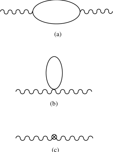
FIG. 1.: One-loop contributions to the correlator $\Pi^{38}_{\mu\nu}$

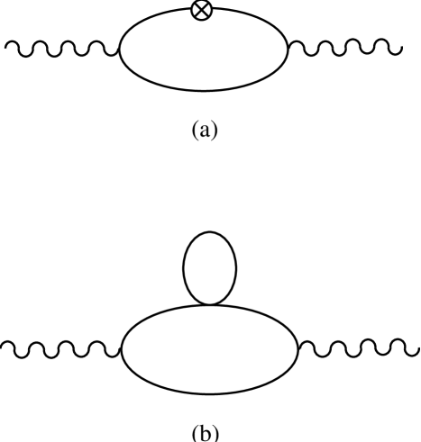
FIG. 2.: Non-contact “insertion” graphs of ${\cal O}(q^{6})$

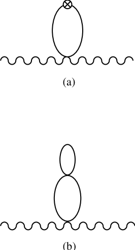
FIG. 3.: Contact “insertion” graphs of ${\cal O}(q^{6})$

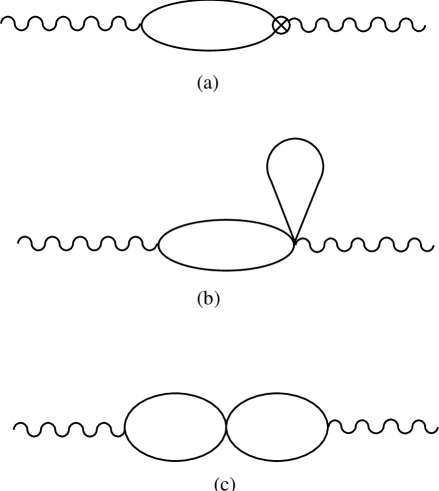
FIG. 4.: Non-contact, non-“insertion” graphs of ${\cal O}(q^{6})$

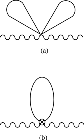
FIG. 5.: Contact, non-“insertion” graphs of ${\cal O}(q^{6})$

FIG. 6.: Tree-level graphs of ${\cal O}(q^{6})$

FIG. 7.: Loop contributions to the correlator $\Pi^{38}(q^{2})$ in units of $10^{-5}$. The solid line is the one-loop result, the dotted and dashed-dotted lines the imaginary and real parts of the full one-loop-plus-two-loop result, respectively.

REFERENCES

[1]Current address: Department of Physics and Mathematical
Physics, University of Adelaide, Adelaide, South Australia 5005, Australia
[2]J. Gasser and H. Leutwyler, Nucl. Phys. B250, 465 (1985).
[3]J. Gasser and H. Leutwyler, Nucl. Phys. B250, 517 (1985).
[4]J. Gasser and H. Leutwyler, Nucl. Phys. B250, 539 (1985).
[5]G. Ecker, “Chiral Perturbation Theory”, Universitat
Wien preprint UWThPh-1994-49, hep-ph/9501357, to appear in
Progress in Particle
and Nuclear Physics 35.
[6]J. Bijnens and F. Cornet, Nucl. Phys. B296, 557 (1988).
[7]J. F. Donoghue, B. R. Holstein and Y. C. Lin, Phys. Rev. D37, 2423 (1988).
[8]E. Golowich and J. Kambour, “Two-Loop Analysis of Vector
Current Propagators in Chiral Perturbation Theory”, Univ. of Mass.
preprint UMHEP-414, hep-ph/9501318, 1995.
[9]G. Ecker, Nucl. Phys. B (Proc. Suppl.) 7A, 78 (1989).
[10]L. J. Ametller, J. Bijnens, A. Bramon and F. Cornet,
Phys. Lett. B276, 185 (1992).
[11]Particle Data Group, “Review of Particle Properties”,
Phys. Rev. D45, 1 (1992).
[12]S. Bellucci, J. Gasser and M. E. Sainio,
Nucl. Phys. B423, 80 (1994).
[13]B. Holdom, R. Lewis and R. R. Mendel, Z. Phys. C63,
71 (1994).
[14]J. Bijnens, A. Bramon and F. Cornet, Phys. Lett. B237, 488 (1990).
[15]J. Bijnens, A. Bramon and F. Cornet, Z. Phys. C46, 599 (1990).
[16]J. Bijnens, Int. J. Mod. Phys. A8, 3045 (1993).
[17]K. Maltman, “The Mixed-Isospin Vector Current Correlator
in Chiral Perturbation Theory and QCD Sum Rules”, University of
Adelaide preprint ADP-95-20/T179, hep-ph/9504237, 1995.
[18]R. Haag, Phys. Rev. 112, 669 (1958).
[19]M. Ademollo and R. Gatto, Phys. Rev. Lett. 13,
264 (1964).
[20]J. Gasser and H. Leutwyler, Ann. Phys. 158, 142 (1984).
[21]G. Passarino and M. Veltmann, Nucl. Phys. B160, 151 (1979); M. Consoli, Nucl. Phys. B160, 208 (1979).
[22]S. Scherer and H. W. Fearing, “Field Transformations and
the Classical Equation of Motion in Chiral Perturbation Theory”,
TRIUMF preprint
TRI-PP-94-64, hep-ph/9408298, 1994.
[23]H. W. Fearing and S. Scherer, “Extension of the Chiral
Perturbation Theory Meson Lagrangian to Order ”, TRIUMF preprint
TRI-PP-94-68, hep-ph/9408346, 1994.
[24]J. F. Donoghue, E. Golowich and B. Holstein, “Dynamics of the
Standard Model”, Cambridge University Press, New York, N.Y., 1992.
[25]G. Ecker, J. Gasser, A. Pich and E. de Rafael, Nucl. Phys. B321, 311 (1989).
[26]J. F. Donoghue, C. Ramirez and G. Valencia, Phys. Rev. D39, 1947 (1989).
[27]R. Dashen, Phys. Rev. 183, 1245 (1969).
[28]K. Maltman and D. Kotchan, Mod. Phys. Lett. A5,
2457 (1990).
[29]J.F. Donoghue, B.R. Holstein and D. Wyler,
Phys. Rev. Lett. 69, 3444 (1992); Phys. Rev. D47,
2089 (1993).
[30]J. Bijnens, Phys. Lett. B306, 343 (1993).
[31]S. Coleman, J. Wess and B. Zumino, Phys. Rev. 177,
2239 (1969); C. G. Callen, S. Coleman, J. Wess and B. Zumino,
Phys. Rev. 177, 2247 (1969).
[32]S. Oneda and G. Oppo, Phys. Rev. 160, 1397 (1967);
T. P. Cheng, Phys. Rev. 162, 1734 (1967);
A. Baracca and A. Bramon, Nuov. Cim. (ser. 10) A69, 613 (1970).
[33]M. A. Shifman, A. I. Vainshtein and V. I. Zakharov,
Nucl. Phys. B147, 519 (1979).
[34]T. Hatsuda, E. M. Henley, T. Meissner and G. Krein,
Phys. Rev. C49, 452 (1994).
[35]M. A. Shifman, A. I. Vainshtein and V. I. Zakharov,
Nucl. Phys. B147, 385, 448 (1979).