April 3, 1995                                                                                       TPR-95-04
Rapidity Dependence of Strange
Particle Ratios
in Nuclear Collisions

Abstract

ABSTRACT

It was recently found [1,2] that in sulphur-induced nuclear collisions at 200 A GeV the observed strange hadron abundances can be explained within a thermodynamic model where baryons and mesons separately are in a state of relative chemical equilibrium, with overall strangeness being slightly undersaturated, but distributed among the strange hadron channels according to relative chemical equilibrium with a vanishing strange quark chemical potential. These studies were made either in a narrow central rapidity window [1] or (in the case of S-S collisions [2]) also using the rapidity-integrated total multiplicities.

We develop a consistent thermodynamic formulation of the concept of relative chemical equilibrium and show how to introduce into the partition function deviations from absolute chemical equilibrium, e. g. an undersaturation of overall strangeness or the breaking of chemical equilibrium between mesons and baryons. We then proceed to test on the available data the hypothesis that the strange quark chemical potential vanishes everywhere, and that the rapidity distributions of all the observed hadrons can be explained in terms of one common, rapidity-dependent function $\mu_{\rm q}(\eta)$ for the baryon chemical potential only. The aim of this study is to shed light on the observed strong rapidity dependence of the strange baryon ratios in the NA36 experiment [3].

Introduction

In the meantime it is almost commonly agreed that fireballs resulting from collisions between heavy ions probably live long enough to establish a state of local thermal and at least relative [1,2] chemical equilibrium. But according to our knowledge no thermodynamic description has been developed yet which gives a quantitative explanation for the different shapes of the rapidity distributions.

We introduce a simple hydrodynamical model of fireballs resulting from S+S collisions at 200 A GeV and allow as a new feature a dependence of the chemical potential on the space-time rapidity. We show that this simple extension increases dramatically the agreement with experimental spectra.

We use the complete set of rapidity distributions for $\pi^{-}$, K^±, K${}^{0}_{s}$, $\Lambda$, $\bar{\Lambda}$ and p-$\bar{\rm p}$ from 200 A GeV/c S+S collisions obtained by the NA35 collaboration [4]. Where applicable we back-extrapolate the published data to the experimental acceptance windows (by inverting the algorithm given by NA35 [4]) since our model is able to take them into account explicitly. In the figures below the index “e” is short for “within experimental acceptance”.

Relative Chemical Equilibrium

J. Rafelski et al. [1] suggested a simple method to test experimental data for possible signals of a QGP in the early stages of heavy ion collisions based on a chemical analysis of the final hadronic composition. The underlying concept rests on the assumption of local thermal and absolute chemical equilibrium with respect to up- and down-quarks, at least in a region near central rapidity. Absolute chemical equilibrium of strange particles is not expected due to the rather high mass of $s\bar{s}$-pairs. Instead one assumes the weaker condition of relative chemical equilibrium: The strange phase space is not fully saturated, but strangeness has been distributed among the available strange hadron channels according to equilibrium fugacities, maximizing the entropy. A convenient way of parametrizing this is by introducing a common saturation factor $0<\gamma_{\rm s}\leq 1$ for both strange quarks and anti-quarks. The abundance of hadrons is then regulated by fugacities $\lambda_{k}$ given by a product of valence quark fugacities multiplied by the factor $\gamma_{\rm s}^{|s_{k}|}$, where $|s_{k}|$ counts the number of strange quarks plus anti-quarks in the respective hadron species.

In [1] the factor $\gamma_{\rm s}$ was introduced heuristically; here we present a rigorous thermodynamic formulation of the concept of relative chemical equilibrium.

In a statistical description of an ideal gas mixture containing $M$ different components, the one particle distribution functions $f_{k}\equiv f_{k}(x,p),\,k=1\ldots M$ contain all of the system’s information. Given sufficient time, this distribution function will evolve to the local equilibrium solution, whose form can be very efficiently derived by maximizing the entropy subject to constraints from conservation laws. For thermal and absolute chemical equilibrium the only constraints are due to the absolutely conserved quantities energy, baryon number and (on the time scale of nuclear reactions) strangeness. (Charge conservation in practice doesn’t play a role in nuclear collisions.) However, if different chemical processes occur at different, well separated time scales, a state of relative chemical equilibrium may arise at intermediate time scales where the fast processes have already equilibrated but the slow ones are still far off equilibrium. This intermediate state can be characterized by additional constraints on the chemical composition which, when implemented into the procedure of entropy maximization, yield the local equilibrium distribution for relative chemical equilibrium.

Let us consider a small fluid cell at freeze-out in its own rest system. Its entropy content can be written as

$${\cal S}=-\sum_{k}\int d\omega\Big{\{}f_{k}\,\ln f_{k}+\theta_{k}\big{(}1-\theta_{k}f_{k}\big{)}\,\ln\big{(}1-\theta_{k}f_{k}\big{)}\Big{\}}$$ (1)

where the integral is over conventional phase space $\int d\omega=\int_{\Delta V}d^{3}x\int\frac{d^{3}p}{(2\pi)^{3}}$, and $\theta_{k}=+1(-1)$ applies to baryons (mesons). The conservation of energy, light ($q$) and strange ($s$) quark flavours in strong interactions leads to the constraints

$$\langle E\rangle=\int d\omega\sum_{k}E_{k}f_{k}\,,\;\;\;\langle Q\rangle=\int d\omega\sum_{k}q_{k}f_{k}\,,\;\;\;-\langle S\rangle=\int d\omega\sum_{k}s_{k}f_{k}\,.$$ (2)

Here $\langle E\rangle$ denotes the cell’s average thermal energy, $\langle Q\rangle$ stands for its average net light quark number (we neglect the small $u$-$d$ mass difference), and $\langle S\rangle$ for its average amount of net strangeness. On the right sides $q_{k}$ and $s_{k}$ count the number of light resp. strange valence quarks in a hadron of species $k$; note that anti-quarks contribute with negative signs.

The concept of a partially saturated strange phase space can be implemented by the additional condition

$$\langle|S|\rangle=\int d\omega\sum_{k}|s_{k}|f_{k}\;.$$ (3)

Since the amounts $\langle S\rangle$ and $\langle|S|\rangle$ of overall strangeness can be specified independently, this allows for a description of both over- and under-saturated strange phase space. We can further parametrize

$$\langle|S|\rangle=\sum_{k}\xi_{k}\,\langle|S|\rangle_{k}^{\rm Eq}\;,$$ (4)

where $\langle|S|\rangle_{k}^{\rm Eq}$ denotes the contribution of the hadron species $k$ to overall strangeness in absolute chemical equilibrium. The factors $\xi_{k}$ represent the degree of population of the strange phase space in each hadronic sector, which may differ from their equilibrium values $\xi_{k}=1$; the range $0<\xi_{k}\leq 1$ corresponds to strangeness suppression. The parametrization (4) explicitly takes into account that quarks are bound into hadrons at freeze-out and allows for a suppression in dependence on their valence quark content.

The most probable distribution function $f_{k}$ can be found by extremizing the functional ${\cal S}[f_{k}]$, subject to the constraints (2, 3). This can be done by means of Lagrangean multipliers $\beta$, $\nu_{q}$, $\nu_{s}$, $\sigma$ and leads to

$$f_{k}=\frac{1}{e^{\beta E_{k}+\nu_{q}q_{k}+\nu_{s}s_{k}+\sigma|s_{k}|}+\theta_{k}}\;.$$ (5)

Inserting (5) into the entropy formula (1) we obtain

$${\cal S}=\beta\langle E\rangle+\sum_{k}(\nu_{\rm q}q_{k}+\nu_{\rm s}s_{k})\langle N_{k}\rangle+\ln\Xi+\sum_{k}\sigma|s_{k}|\langle N_{k}\rangle\;,$$ (6)

where we define the average particle number of species $k$ in the considered volume element $\langle N_{k}\rangle=\int d\omega f_{k}$ and

$$\ln\Xi=\sum_{k}\theta_{k}\int d\omega\ln\left(1+\theta_{k}e^{-(\beta E_{k}+(\nu_{\rm q}q_{k}+\nu_{\rm s}s_{k})+\sigma|s_{k}|)}\right)\;.$$ (7)

The limit $\sigma\to 0$ corresponds to neglecting the additional condition (3) in the extremization procedure. In this case we recover from (7) the expression for the grand canonical partition function in absolute chemical equilibrium.

It can be easily shown that $\ln\Xi$ generates all thermodynamic quantities ($\alpha_{k}\equiv(\nu_{\rm q}q_{k}+\nu_{\rm s}s_{k})+\sigma|s_{k}|$):

$$-\frac{\partial}{\partial\beta}\ln\Xi\Big{|}_{\alpha_{k},V}=\langle E\rangle\,,\;\;\;-\frac{\partial}{\partial\alpha_{k}}\ln\Xi\Big{|}_{\beta,V}=\langle N_{k}\rangle\,,\;\;\;T\frac{\partial}{\partial V}\ln\Xi\Big{|}_{\alpha_{k},T}=p\,.$$ (8)

Hence it is a thermodynamic potential. As usual we identify $\beta=\frac{1}{T}$ and $\alpha_{k}=-\frac{\mu_{k}}{T}$. The chemical potentials in absolute chemical equilibrium

$$\mu_{k}^{\rm Eq}=-T(\nu_{\rm q}q_{k}+\nu_{\rm s}s_{k})$$ (9)

are connected with $\mu_{k}$ via

$$\mu_{k}=\mu_{k}^{Eq}-T\sigma|s_{k}|\equiv\mu_{k}^{Eq}+\tilde{\sigma}|s_{k}|\;,$$ (10)

where we defined $\tilde{\sigma}=-T\sigma$.

In Boltzmann approximation we can determine the suppression factors $\xi_{k}$ by comparing (3) and (4) as $\xi_{k}=e^{(\beta\tilde{\sigma}|s_{k}|)}$. They are directly related to the saturation factor $\gamma_{\rm s}$ via $\xi_{k}=\gamma_{\rm s}^{|s_{k}|}$:

$$0<\gamma_{\rm s}^{|s_{k}|}=\xi_{k}=(e^{\beta\tilde{\sigma}})^{|s_{k}|}\leq 1\;.$$ (11)

An overall suppression of the strange quark phase space has no influence on the thermodynamic relations (8); it only enters into the relation (1) for the entropy. If decomposed into particle specific contributions ${\cal S}=\sum_{k}{\cal S}_{k}$ we immediately see that each component receives an additional contribution $-|s_{k}|\ln\gamma_{\rm s}\langle N_{k}\rangle$.

The starting point of our formalism were the suppression factors $\xi_{k}$ weighting each hadron species separately. As a consequence of the entropy maximization, however, we automatically arrived at the concept of relative chemical equilibrium with one common factor $\gamma_{\rm s}$. This justifies a posteriori the parametrization of Rafelski et al. [1].

The procedure is easily generalized to allow for a meson-baryon non-equilibrium as suggested in the last of Refs. [1]. This might be necessary if processes of the type $M$+$M$ $\leftrightarrow$ $\bar{B}$+$B$ are slow. Let us assume that baryons are in absolute chemical equilibrium and mesons are not. This requires the inclusion of the additional constraint

$$\langle M\rangle=\sum_{k}\,\mbox{$\frac{1}{2}$}(1-\theta_{k})\,\int\,d\omega\,f_{k}\;,$$ (12)

where again we can parametrize in the same spirit as (4)

$$\langle M\rangle=\sum_{k}\,\mbox{$\frac{1}{2}$}(1-\theta_{k})\,\xi^{\rm m}_{k}\,\langle N_{k}\rangle^{\rm Eq}\;.$$ (13)

Combining (3) and (12) we find the relative equilibrium distribution

$$f_{k}=\gamma_{\rm s}^{|s_{k}|}\,\gamma_{\rm m}^{\frac{1}{2}(1-\theta_{k})}\,f_{k}^{\rm Eq}\;,$$ (14)

where in Boltzmann approximation $\xi_{k}^{\rm m}$ and $\gamma_{\rm m}$ are related by $\xi_{k}^{\rm m}=\gamma_{\rm m}^{\frac{1}{2}(1-\theta_{k})}$. The case where also the baryons are suppressed or enhanced relative to their equilibrium abundance can be treated in an analogous way.

Calculating the Spectra

For the momentum spectra of hadrons emitted from the fireball at freeze-out we use the simple hydrodynamical model developed by E. Schnedermann et al. [5]. It is based on the idea of a thermal distribution with one freeze-out temperature $T_{\rm f}$ characterizing the instant at which fluid cells loose their thermal contact to the fireball. Experiments find similar exponential slopes in all $m_{\bot}$-spectra, independent of the rapidity window [4]. This supports the interpretation of freeze-out at one common and constant temperature.

The general expression for the invariant momentum distribution is [6]

$$E\frac{d^{3}N}{dp^{3}}=\frac{g}{(2\pi)^{3}}\int_{\sigma_{\rm f}}f(x,p)\,p^{\nu}d^{3}\sigma_{\nu}\;,$$ (15)

where $g$ is the spin degeneracy of the hadrons under consideration and $\sigma_{\rm f}$ is the 3-dimensional freeze-out hypersurface in space-time, along which the condition $T=T_{\rm f}$ is fulfilled. We choose a cylindrical coordinate system $(r,\phi,z)$ which best reflects the global symmetries of the expanding fireball and obtain for the normal vector of the freeze-out surface

$$d^{3}\sigma_{\nu}=\left(1,-\frac{\partial t_{\rm f}}{\partial r}\cos\phi,-\frac{\partial t_{\rm f}}{\partial r}\sin\phi,-\frac{\partial t_{\rm f}}{\partial z}\right)\,rdr\,d\phi\,dz\;.$$ (16)

In an azimuthally symmetric geometry of this kind it is practical to decompose the velocity field in the following way [7]:

$$u^{\nu}=\left(\cosh\rho\,\cosh\eta,\hat{e}_{\bot}\sinh\rho,\cosh\rho\,\sinh\eta\right)\;.$$ (17)

Here $\eta=\eta(t,r,z)$ is the longitudinal flow rapidity by which each volume element on the z-axis moves relative to the center of mass, and $\rho=\rho(t,r,z)$ is the rapidity corresponding to the transverse flow of the volume element at position $(r,z)$ as seen from a reference point at $z$ on the beam axis moving with the local flow velocity there. The 4-momentum can be parametrized in terms of rapidity $y$ and transverse mass $m_{\bot}=\sqrt{p_{\bot}^{2}+m_{0}^{2}}$ as

$$p^{\nu}=(m_{\bot}\cosh y,p_{\bot}\cos\phi_{\rm p},p_{\bot}\sin\phi_{\rm p},m_{\bot}\sinh y)\;.$$ (18)

After suitably orienting the coordinate system we obtain in Boltzmann-approximation:

$$\frac{d^{2}N}{\,dy\,dm_{\bot}^{2}} = \frac{g}{4\pi}\,m_{\bot}\int_{t_{\rm f}}dz\,r\,dr\,e^{\mu/T}\,e^{-\tilde{\alpha}\cosh(\eta-y)}$$ (20)

$$\times\left\{\left(\cosh y-\sinh y\frac{\partial t_{\rm f}}{\partial z}\right){\rm I}_{0}(\alpha)-\frac{p_{\bot}}{m_{\bot}}\frac{\partial t_{\rm f}}{\partial r}\,{\rm I}_{1}(\alpha)\right\}\;,$$

where $\tilde{\alpha}=(m_{\bot}/T)\cosh\rho$ and $\alpha=(p_{\bot}/T)\sinh\rho$. The 2-dimensional integration extends along the curve determined by all points $(r,z)$ which at time $t_{\rm f}(r,z)$ satisfy $T(t_{\rm f}(r,z),r,z)=T_{\rm f}$.

For further evaluation we introduce new variables and transform $(t,r,z)$ into $(\tau,r,Y)$ with the longitudinal proper time $\tau=\sqrt{t^{2}-z^{2}}$ and the space-time rapidity $Y=0.5\ln\left[(t+z)/(t-z)\right]$. Numerical simulations of the space-time evolution of the hot zone in ultrarelativistic nuclear collisions show an almost linear velocity profile in beam direction [8]. Hence a boost invariant scenario, if restricted to the fireball’s finite extension, is a good approximation for the longitudinal fluid dynamics and leads to $Y\equiv\eta$, i.e. the identity of space-time rapidity $Y$ and fluid rapidity $\eta$. The partial derivatives $\frac{\partial t_{\rm f}}{\partial r}$ and $\frac{\partial t_{\rm f}}{\partial z}$ are easily evaluated if we parametrize the freeze-out hypersurface by a proper time surface $\tau_{\rm f}(r)$: $t_{\rm f}(r,z)=\sqrt{\tau_{\rm f}^{2}(r)+z^{2}}$. In doing so we simultaneously express the invariance of the decoupling process against longitudinal boosts and obtain for the rapidity distribution using $z=\tau_{\rm f}(r)\sinh\eta$:

$$\frac{dN}{dy} = \frac{g}{4\pi}\,\int_{m_{\bot}^{\rm lo}}^{m_{\bot}^{\rm hi}}\,dm_{\bot}^{2}\,\int_{-\tilde{\eta}}^{\tilde{\eta}}\,d\eta\int_{0}^{R_{\rm f}}\,dr\,\tau_{\rm f}(r)\,r\,e^{\mu/T}e^{-\tilde{\alpha}\cosh(y-\eta)}$$ (21)

$$\times \left(m_{\bot}\cosh(y-\eta)\,{\rm I}_{0}(\alpha)-p_{\bot}\frac{\partial\tau_{\rm f}(r)}{\partial r}\,{\rm I}_{1}(\alpha)\right)\;.$$ (22)

In this expression $m_{\bot}^{\rm lo},\;m_{\bot}^{\rm hi}$ denote the experimental limits in which the spectrum was measured, the freeze-out radius is called $R_{\rm f}$ and the longitudinal extent of the fireball is fixed via the finite interval $-\tilde{\eta}\ldots\tilde{\eta}$. We will later use the approximation where we assume transversally instantaneous freeze-out ($\frac{\partial\tau_{\rm f}(r)}{\partial r}=0$) and replace the transverse flow velocity profile by its radial average. In this case eq. (21) reduces to the simpler form

$$\frac{dN}{dy}=\frac{g\,\tau_{\rm f}R_{\rm f}^{2}}{8\,\pi}\,\int_{m_{\bot}^{\rm lo}}^{m_{\bot}^{\rm hi}}\,dm_{\bot}^{2}\,m_{\bot}\,{\rm I}_{0}(\alpha)\int_{-\tilde{\eta}}^{\tilde{\eta}}d\eta\,\cosh(y-\eta)\,e^{\mu/T}\,e^{-\tilde{\alpha}\cosh(y-\eta)}\;.$$ (23)

The Parametrization of the Chemical Potential

Spectra of hadrons $k$ containing $q_{k}$ up or down valence quarks and $s_{k}$ strange quarks are fully characterized, besides the two flow components, by the temperature $T=1/\beta$ and the fugacity $\lambda_{k}=\gamma_{\rm s}^{|s_{k}|}\>e^{\beta\mu_{\rm s}s_{k}}\>e^{\beta\mu_{\rm q}q_{k}}$ (see the section on relative chemical equilibrium).

J. Sollfrank et al. [2] found in a chemical analysis of S+S collisions, using rapidity integrated total multiplicities, a vanishing chemical potential $\mu_{\rm s}\approx 0$ of the strange quarks and an almost complete saturation $\gamma_{\rm s}\approx 1$ of the phase space of strange particles. It is doubtful that these parameters can be established in a purely hadronic environment, therefore we adopt as a working hypothesis the formation of a QGP in the early stages of the collision. This leads to $\mu_{\rm s}=0$ independent of $T$, $\mu_{\rm q}$ and also of $r$ and $z$ (resp. $\eta$). We further assume that these values are maintained during the process of hadronisation. (For a detailed discussion of this assumption see the last reference [1].) Our objective is to completely fix the baryon chemical potential by using only the hyperon spectra, and then test whether other measured hadron distributions can be reproduced in shape as well as normalization.

The width of the rapidity distributions is mainly determined by the longitudinal flow component. It can be extracted with very little sensitivity to $T$ and transverse flow from the shape of the pion rapidity spectrum [5]. In this way we obtain a maximum fluid rapidity (see (23)) of $\tilde{\eta}=1.75$. In a first attempt we neglect the transverse flow ($\rho=0$) and choose $T=200\pm 20\,{\rm MeV}$, consistent with the slope of transverse mass distributions. We are aware of the fact that this value is too high to be interpreted as the real freeze-out temperature directly, but in a hadron gas a temperature of this order seems to be necessary to ensure strangeness neutrality [1,2,9].

Both protons and $\Lambda$-hyperons possess a quite broad rapidity distribution and peak in the fragmentation regions. This suggests a concave parametrization for $\mu_{\rm q}(\eta)$. We checked several possibilities and found that a quartic ansatz of the form

$$\mu_{k}(\eta)=(\mu_{\rm q}^{0}+A\,\eta^{4})\,q_{k}\;,\quad\mu_{\rm q}^{0}=59\pm 11\,{\rm MeV}\;,\quad A=11.5\pm 0.5\,{\rm MeV}$$ (24)

together with $\tilde{\eta}=1.75$ is able to describe both $\Lambda$- and $\bar{\Lambda}$-distributions simultaneously (Fig. 1 a-b).

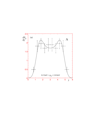
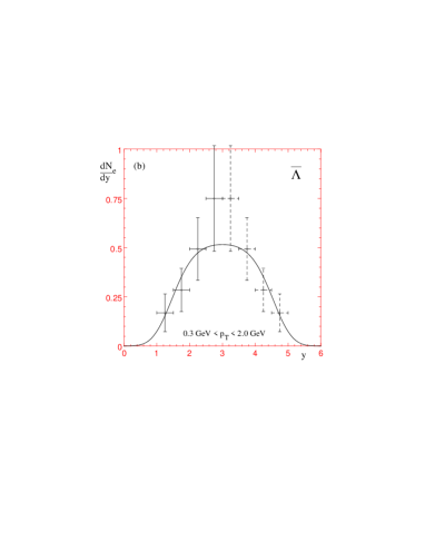
FIG. 1.: Rapidity distribution of $\Lambda$- and $\bar{\Lambda}$-hyperons. The theoretical curve with our quartic parametrized chemical potential is fitted to data of NA35 S+S 200 A GeV [4].

The central data points of the $\bar{\Lambda}$’s are barely reached only, but they have the largest error bars. We used the fact that both spectra are measured in the same $p_{\bot}$-window, whereby the integrals over the boostangle $\eta$ cancel in the ratio of the distributions at midrapidity. From the central normalization of the $\Lambda$-distribution we also determine $\tau_{\rm f}R_{\rm f}^{2}=20\pm 4\>{\rm fm}^{3}$. The contribution from $\Sigma^{0}$ decays to the $\Lambda$ spectrum is taken into account in the theory by an additional degeneracy factor of 2.

The Results

Integrating $\mu(\eta)$ over the fluid (or space-time) rapidity $\eta$, we determine an average baryochemical potential of $\bar{\mu}_{\rm B}=3\bar{\mu}_{\rm q}=(240\pm 40)\>{\rm MeV}$. This is in good agreement with the findings of J. Sollfrank et al. [2], $\mu_{\rm B}=(264\pm 72)\>{\rm MeV}$ who used a chemical analysis of the $4\pi$-integrated multiplicities. But the most important result is that we are able to also reproduce all other available hadron spectra (Fig. 2 a-d). Not only the shape of the distributions coincides with the experiment, but also (except for the pions which will be discussed separately below) the normalization is reproduced correctly without adjustments. (Due to error propagation some of our kaon curves may, however, have up to 35% uncertainty in normalization.) This is a dramatic improvement over the results obtained in Ref. [5] with rapidity independent chemical potentials.

FIG. 2.: Rapidity distribution of kaons and protons in comparison with data of NA35 for S+S at 200 A MeV [4]. The absolute normalizations are not fitted, but calculated using $T=200\,{\rm MeV}$, $\tilde{\eta}=1.75$ and the quartic parametrization for the chemical potential. Figure e) represents the proton distribution assuming an undersaturation of overall strangeness $\gamma_{\rm s}=0.75$.

The calculated proton distribution (Fig. 2 d) is clearly narrower than the experimental result, moreover the normalization is a little too low. The first feature is expected because protons are unlikely to be completely thermalized, especially in the extreme kinematic domains, due to nuclear transparency in particular in the transverse nuclear surface. On the other hand a slight undersaturation of the overall strangeness by a factor $\gamma_{\rm s}=0.75$ fully corrects the normalization problem (Fig. 2 e). Since all the other hadrons carry only one $s$- or $\bar{s}$-quark, this leaves the spectra unchanged, if the factor $\tau_{\rm f}\,{\rm R}_{\rm f}^{2}$ is increased correspondingly by a factor $4/3$.

We conclude from this agreement with experiment that a thermodynamic description will work well in a rather wide rapidity interval if dependencies of the thermodynamic parameters on rapidity are taken into consideration. The interesting observation here is that it is apparently sufficient to consider a rapidity dependence of the baryon chemical potential, keeping $T$, $\mu_{\rm s}=0$ and $\gamma_{\rm s}$ fixed. On the other hand this means that one has to be careful when applying thermodynamic models to data which are not restricted to a narrow and central kinematic domain, because then this rapidity dependence is integrated over with different weights for different particle species. As a further result the strong dependence of strange particle ratios on the rapidity window which was observed by NA36 in S+Pb collisions [3] can be qualitatively explained by our model in a very natural way.

FIG. 3.: Deviation from local strangeness neutrality. The quantity $\epsilon$ (23) is plotted as a function of space-time rapidity $\eta$ for $T=200\,{\rm MeV}$, $\gamma_{\rm s}=1$ and the parametrization (22) for the chemical potential. The dashed curve is calculated using a mass cut in the hadronic resonance spectrum at $m_{\rm cut}=1.8\;{\rm GeV}$, the solid one represents $m_{\rm cut}=2.0\;{\rm GeV}$.

To test the important condition of strangeness neutrality we define

$$\epsilon(\eta)=\frac{\langle\bar{s}\rangle(\eta)-\langle s\rangle(\eta)}{\langle s\rangle(\eta)}$$ (25)

as a measure for the local deviation. Fig. 3 shows the result plotted in the relevant range of $\eta$ for two different cuts in the hadron mass spectrum. We recognize that strangeness neutrality can not be guaranteed locally, though $\epsilon(\eta)$ is flat and almost zero in $-1.2\leq\eta\leq 1.2$. On the other hand the clear experimental differences between the rapidity densities of different hadrons can be seen as an indication that a violation might indeed be realized locally. In a global sense, i.e. integrated over rapidity $\eta$, we obtain

$\gamma_{\rm s}$ 1.0 0.75 $m_{\rm cut}$ [GeV] 1.8 2.0 1.8 2.0 $\epsilon_{\rm global}$ 0.03 -0.16 0.09 -0.09   .

If we take into consideration the uncertainties in temperature, chemical potential and a possible asymmetry in the data tables between meson and baryon resonances of high rest masses (due to different efficiencies for their identification), we conclude that we have no problem in ensuring at least global strangeness neutrality.

Transverse flow

Despite this very good and consistent agreement of our model with experiment this comparison has one substantial shortcoming: the assumed temperature is really too high for consistency of the model. The spatial overlap of hadrons at $T=200\,{\rm MeV}$ is quite large already, and indeed lattice QCD simulations now firmly predict a QGP phase transition already at $T=150\,{\rm MeV}$ [10]. The assumption of a system of non-interacting particles freezing out at $T=200\,{\rm MeV}$ is thus more than dubious. These were the decisive reasons for the authors of [2,5] to conclude that the flat slope of the observed $m_{\bot}$-spectra is partially caused by a blueshift due to collective transverse flow. Already $\rho\simeq 0.3$ reduces the true temperature from $T\simeq 200\,{\rm MeV}$ to $T\simeq 150\,{\rm MeV}$, and we will use this average value in the following considerations.

FIG. 4.: Rapidity distributions of kaons and protons in comparison with data of NA35 S+S at 200 A MeV [4]. The absolute normalizations in the cases c)-e) are not fitted, but calculated using $T=150\,{\rm MeV}$, $\tilde{\eta}=1.75$ and the quartic parametrization for the chemical potential. Please note that $\gamma_{\rm s}=\gamma_{\rm m}=1$ was assumed.

We again determine $\mu_{\rm q}^{0}$ and $A$ as described above from the hyperon spectra, now leading to $A=8.0\pm 0.5\,{\rm MeV}$ and $\mu_{\rm q}^{0}\simeq 43\,{\rm MeV}$. The lower temperature reduces the thermal smearing whereby all the theoretical rapidity spectra become somewhat narrower. The calculated proton distribution now fits the experimental data (except for the disagreement near the projectile and target rapidities discussed already above), even with $\gamma_{\rm s}=1$ (Fig. 4 c).

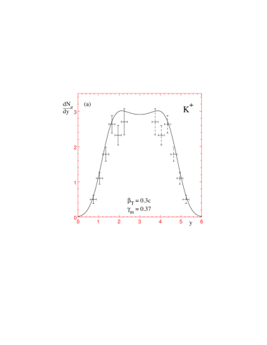
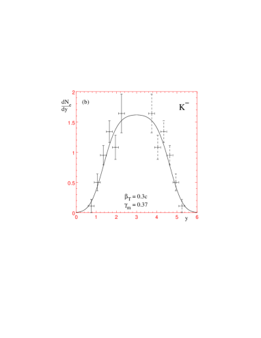
FIG. 5.: Rapidity distribution of kaons in comparison with data of NA35 S+S 200 A GeV [4]. The theoretical curve is calculated using $T=150\,{\rm MeV}$, $\tilde{\eta}=1.75$ and $\gamma_{\rm m}=0.37$.

With kaons, however, we now have a serious problem: Although the shape is correct for all three charge states, the theoretical normalization exceeds the data by a common factor of approximately 2.7 (Fig. 4 d-e). As a consequence the theoretical spectra also strongly violate overall strangeness neutrality. However, there is a very simple remedy for this. Following the ideas first laid out in Ref. [1d] and worked out in Ref. [1c], one can assume a breaking of the relative chemical equilibrium between the mesons and baryons by introducing a meson/baryon suppression factor $\gamma_{\rm m}<1$. It is quite a surprise that by choosing $\gamma_{\rm m}=0.37$ we can simultaneously correct the normalization of all kaon spectra (Fig. 5) and recover global strangeness neutrality:

$m_{\rm cut}$ [GeV] 1.8 2.0 $\epsilon_{\rm global}$ -0.05 -0.13 $\;.$

Excess Entropy

In both analyses (with and without transverse flow) we used the pion rapidity spectra to extract the maximum flow rapidity, but did not check their normalization. It turns out that in both cases we seriously underpredict the pion multiplicity (typically by a factor 2-3). While in the case with transverse flow and $\gamma_{\rm s}=\gamma_{\rm m}=1$ we are not too much off (see fig. 6 a), after introducing the meson suppression factor $\gamma_{\rm m}=0.37$ (thereby recovering the correct kaon normalization and strangeness neutrality) we again obtain by a factor 2-3 too few pions. This feature in the data (too many pions compared to a hadron gas in relative chemical equilibrium) was observed before [1,2,11] and is confirmed by the completely different experimental analysis reported by M. Gaździcki at “Strangeness ’95” [12]. It is interpreted as an indication for excess entropy in the data which might originate from the gluonic entropy in the QGP [1]. Why this extra entropy shows up mainly in the form of pions is not yet clear. Their nature as nearly massless chiral goldstone bosons may play a role here, but no dynamical explanation has been given so far.

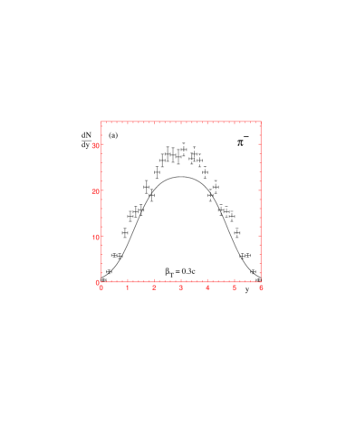
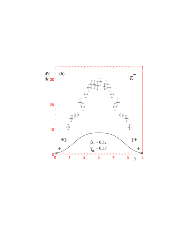
FIG. 6.: Rapidity distribution of pions. The theoretical curve with our quartic parametrized chemical potential and a transverse flow of $\beta_{\rm T}=\tanh\rho=0.3$ is compared to data of NA35 S+S 200 A GeV [4]. Figure b) is based on a meson baryon suppression factor $\gamma_{\rm m}=0.37$.

Summary

We showed that a rather simple thermodynamic model with a suitably parametrized rapidity dependent baryochemical potential can reproduce the measured distributions of strange particles resulting from S+S collisions at 200 A GeV. Consistency was achieved with the shape as well as with the normalization of the rapidity spectra. Our phenomenologically motivated ansatz was not able to guarantee strangeness neutrality locally, but globally strangeness was conserved. One further result of our model was a qualitative explanation of the strong dependence of strange particle ratios on the chosen kinematic window.

Resonance decays have not been taken into consideration so far, but will be considered in the future. They are expected to mostly affect the pion spectra, but also kaons could be influenced in a non-negligible way. We have conscisously kept $\mu_{\rm s}=0$ and $\gamma_{\rm s}$, $\gamma_{\rm m}$ as rapidity-independent, because otherwise a unique determination of such a large set of free parameter functions would be impossible to fix from the available data.

REFERENCES

-
-
[1]
J. Rafelski, Phys. Lett. 262 (1991) 333;
J. Rafelski, Nucl. Phys. A544 (1992) 279;
J. Letessier, A. Tounsi, and J. Rafelski, Phys. Lett. 292 (1992) 417;
J. Letessier et al., Phys. Rev. D51 (1995), in press. - [2] J. Sollfrank, M. Gaździcki, U. Heinz and J. Rafelski Z. Phys. C61 (1994) 659.
-
[3]
NA36 collaboration:
E. Anderson et al., Nucl. Phys. A566 (1994) 217c;
E. Anderson et al., Phys. Lett. B327 (1994) 433. -
[4]
NA35 collaboration:
T. Alber et al., Z. Phys. C64 (1994) 195;
J. Bächler et al., Phys. Rev. Lett. 72 (1994) 1419;
J. Bächler et al., Z. Phys. C58 (1993) 367. -
[5]
E. Schnedermann and U. Heinz, Phys. Rev. Lett.
69 (1992) 2908;
E. Schnedermann and U. Heinz, Phys. Rev. C47 (1993) 1738;
E. Schnedermann, J. Sollfrank and U. Heinz, Phys. Rev. C48 (1993) 2462;
E. Schnedermann and U. Heinz, Phys. Rev. C50 (1994) 1675;
E. Schnedermann et al., in: ‘Particle Production in Highly Excited Matter’,
(Plenum, New York, 1992, H. H. Gutbrod and J. Rafelski, Eds.), p. 175ff. - [6] F. Cooper and G. Frye, Phys. Rev. D10 186.
- [7] P. V. Ruuskanen, Acta Phys. Pol. B18 (1987) 551.
- [8] T. Csörgö et al., Phys. Lett. B222 (1989) 115.
- [9] J. Cleymans and H. Satz, Z. Phys. C57 (1993) 135.
- [10] F. Karsch, in “Quark Matter ’95”, (A. Poskanzer et al., Eds.), Nucl. Phys. A (1995), in press.
- [11] J. Letessier et al., Phys. Rev. Lett. 70 (1993) 353.
- [12] M. Gaździcki, Z. Phys. C, in press, and talk given at “Strangeness ’95”.