BNL-61590

ISU-HET-95-1

March 1995

LOOKING FOR ${\cal CP}$ VIOLATION IN $W$ PRODUCTION AND DECAY

S. Dawson^(a) and G. Valencia^(b)
(a) Physics Department, Brookhaven National Laboratory, Upton, NY 11973
^(b) Department of Physics and Astronomy, Iowa State University, Ames IA 50011

We describe ${\cal CP}$ violating observables in resonant $W^{\pm}$ and $W^{\pm}$ plus one jet production at the Tevatron. We present simple examples of ${\cal CP}$ violating effective operators, consistent with the symmetries of the Standard Model, which would give rise to these observables. We find that ${\cal CP}$ violating effects coming from new physics at the $TeV$ scale could in principle be observable at the Tevatron with $10^{6}$ $W^{\pm}$ decays.

1 Introduction

The origin of ${\cal CP}$ violation remains one of the unsolved questions in particle physics. It is therefore very important to search for signals of ${\cal CP}$ violation in all the experimentally accessible systems. The Tevatron has now accumulated a sample of about $50000$ $W^{\pm}$ events and samples of $10^{7}$ events should be possible eventually. This makes it timely to think of testing ${\cal CP}$ violation in $W^{\pm}$ production and decay.

In this paper we study the processes $p\overline{p}\rightarrow W^{\pm}$ and $p\overline{p}\rightarrow W^{\pm}\ +1{\rm~{}jet}$. Some ${\cal CP}$ odd observables in these processes involve the polarization of the $W^{\pm}$ boson. It is, therefore, convenient to allow the $W^{\pm}$ to decay leptonically into $\ell^{\pm}\nu$ pairs and study the complete processes $p\overline{p}\rightarrow\ell^{\pm}\nu\ +\ {\rm~{}0~{}or~{}1~{}jet}$. In this way we recover some information on the direction of the vector boson polarization by measuring the charged lepton momentum. Although it is also possible to construct observables for hadronic $W^{\pm}$ decays, we will not consider that case in this paper to avoid the complications of hadronization.

In this paper we adopt the strategy of searching for small ${\cal CP}$ violating contributions to a dominant process instead of looking for potentially larger effects in rare processes. We therefore limit our discussion to ${\cal CP}$ odd observables in the decay chains

$$p\overline{p}\rightarrow W^{\pm}\ +\ {\rm~{}0~{}or~{}1~{}jet}\rightarrow\ell^{\pm}\nu\ +\ {\rm~{}0~{}or~{}1~{}jet}$$ (1)

and consequently we study these processes in the narrow width approximation. We concentrate on the dominant parton subprocesses, ignoring for example, top-quark distribution functions in the proton, ${\cal CP}$ violation in the parton distribution functions, and ${\cal CP}$ violation that occurs only at higher twist.

It is, of course, possible that there are ${\cal CP}$ violating effects that vanish within our approximation. An example in $\ell\nu$ production arises from the interference of the one-loop electroweak corrections to the resonant $W^{\pm}$ Standard Model amplitude with a non-resonant ${\cal CP}$ violating four-fermion new physics interaction. This example has been studied by Barbieri et. al [3].

It should be clear that the ${\cal CP}$ odd observables that we discuss are predominantly sensitive to ${\cal CP}$ violation in the $udW$ vertex and in the $W\ell\nu$ vertex and these are the same vertices which are probed in pion decay $\pi\rightarrow\ell\nu$.However, there are several scenarios under which the direct $W$ production and decay processes are more sensitive to ${\cal CP}$ violation than the corresponding pion decay. This is true in the examples we discuss for at least one of the following reasons:

• The new physics (at a high energy scale $\Lambda$) that violates ${\cal CP}$ contributes to the effective $W(q)f\overline{f^{\prime}}$ vertex in a way proportional to $(q^{2}/\Lambda^{2})^{n}$, $n\geq 1$. Since $q^{2}\ll\Lambda^{2}$, the leading contribution will be for $n=1$. The effects from the new physics on direct $W$ production and decay are therefore enhanced over effects in pion decay by at least a factor $M_{W}^{2}/m_{\pi}^{2}\sim 3.5\times 10^{5}$.

• The absorptive phases needed to construct $T$-even observables are larger in $W$ production and decay. An example is the case where the absorptive phase is due to a rescattering of the final state with electroweak strength. This would be the case if the new physics generates an effective four-fermion interaction that contributes to the $Wf\overline{f^{\prime}}$ vertex at the one-loop level. In this case, the absorptive phase introduces an additional suppression factor of order $\Gamma_{W}/M_{W}\sim 3\%$ for direct $W$ production and decay, whereas it introduces a suppression factor of order $G_{f}m_{\pi}^{2}\sim 10^{-8}$ for pion decays.

• Processes with a sufficient number of independent four-vectors to construct $T$-odd triple products are suppressed at low energy. In direct $W$ production and decay we can look for events with one jet, suppressed by a factor of $\alpha_{s}$ with respect to the lowest order QCD process. In pion decays we need a three body decay mode with the measurement of a polarization or a four body decay mode. Three body decay modes are four orders of magnitude smaller than $\pi\rightarrow\ell\nu$ and polarization measurements are extremely difficult. Four body decay modes are nine orders of magnitude smaller than $\pi\rightarrow\ell\nu$.

Kaon decay experiments tell us that the ${\cal CP}$ violating phases in the Standard Model are extremely small. In addition, ${\cal CP}$ odd observables in the standard model vanish in the limit of massless light fermions, and are thus even smaller at higher energies [4]. The Standard Model does not produce a sufficiently large ${\cal CP}$ violating signal to be observed in the processes we study [5]. Popular extensions of the standard model in the context of ${\cal CP}$ violation include multi-Higgs models. In these models ${\cal CP}$ violation is also proportional to fermion masses and thus negligible in processes like $d\overline{u}\rightarrow W^{-}\rightarrow e^{-}\overline{\nu}$ at high energy. We will, therefore, work from the assumption that studies of ${\cal CP}$ violation at colliders will only be sensitive to non-Standard Model sources. Furthermore, we will not consider a specific model for ${\cal CP}$ violation, but instead we will use an effective Lagrangian approach to parameterize possible ${\cal CP}$ violating operators. We will further assume that the origin of these operators lies in the physics that breaks the electroweak symmetry. With a linear realization of the symmetry breaking and a light Higgs, all the operators of dimension $6$ have been given in Refs. [6, 7]. With a non-linear realization of the symmetry breaking sector, anomalous fermion-gauge-boson couplings have been described in Ref. [8]. Here we consider just a few of these operators to illustrate the physics, but it should be obvious that a similar analysis can be applied to other operators.

There have been a number of studies of ${\cal CP}$ violation at colliders that concentrate on effects due to the top-quark or multiple $W$ production Ref. [9]. We concentrate on single $W$ production and complement the work of Refs.[3, 10]. We will not discuss detector issues at all, except to make the obvious statement that the detector must be “${\cal CP}$-blind” in order to carry out these studies. We limit ourselves to offer a “proof in principle” that ${\cal CP}$ violation could be observed in $W^{\pm}$ decays at the Tevatron.

2 $p\overline{p}\rightarrow W^{\pm}X\rightarrow\ell^{\pm}\nu X$

We assume that the proton and anti-proton beams are unpolarized, and that the polarization of the lepton is not measured. In this case, it is only possible to construct $T$-even observables for this reaction. Some ${\cal CP}$ odd observables have been listed in Ref. [5]. Here we discuss a few simple observables of this type in the context of a ${\cal CP}$ violating four-fermion interaction due to physics beyond the minimal standard model.

Under a ${\cal CP}$ transformation, the reaction $p(\vec{p})\overline{p}(-\vec{p})\rightarrow\ell^{+}(\vec{q})\nu X$ transforms into $p(\vec{p})\overline{p}(-\vec{p})\rightarrow\ell^{-}(-\vec{q})\overline{\nu}\overline{X}$. Here we work in the $p\overline{p}$ center of mass frame and denote by $\overline{X}$ the ${\cal CP}$ conjugate of $X$. Also, we have only considered those kinematic variables that can be observed, in this case the momenta of the beam and the lepton. It is conventional to take the $z$-axis as being the direction of the proton beam, and to use rapidity and transverse momentum as the kinematical variables. Recalling that the lepton rapidity is given by (all variables in the $p\overline{p}$ center of mass):

$$y_{\ell}={1\over 2}\log\biggl{(}{E_{\ell}+q_{z\ell}\over E_{\ell}-q_{z\ell}}\biggr{)}$$ (2)

and the lepton transverse momentum by:

$$p_{T\ell}=|\vec{q}\sin\theta|$$ (3)

where $\theta$ is the angle between the proton and lepton momenta in the lab frame, one can see that under a ${\cal CP}$ transformation

$$y_{\ell^{-}}\stackrel{{\scriptstyle{\cal CP}}}{{\longleftrightarrow}}-y_{\ell^{+}},\ \ \ p_{T\ell^{-}}\stackrel{{\scriptstyle{\cal CP}}}{{\longleftrightarrow}}p_{T\ell^{+}}$$ (4)

In terms of these variables we can, therefore, construct ${\cal CP}$-odd observables such as:

$$\tilde{R}_{1} \equiv {{\sigma}^{+}-{\sigma}^{-}\over{\sigma}^{+}+{\sigma}^{-}}$$

$$\tilde{R}_{2}(y_{0}) \equiv {{d{\sigma}^{+}\over dy_{\ell}}\mid_{y_{\ell}=y_{0}}-{d{\sigma}^{-}\over dy_{\ell}}\mid_{y_{\ell}=-y_{0}}\over{d{\sigma}^{+}\over dy_{\ell}}\mid_{y_{\ell}=y_{0}}+{d{\sigma}^{-}\over dy_{\ell}}\mid_{y_{\ell}=-y_{0}}}$$

$$\tilde{R}_{3}(p_{T}) \equiv {{d{\sigma}^{+}\over dp_{T}}-{d{\sigma}^{-}\over dp_{T}}\over{d{\sigma}^{+}\over dp_{T}}+{d{\sigma}^{-}\over dp_{T}}},$$ (5)

where ${\sigma}^{\pm}$ refers to $\sigma(p\overline{p}\rightarrow\ell^{\pm}\nu X)$. Of course, it is also possible to construct ${\cal CP}$ odd observables based on more complicated correlations, but we will not pursue that route in this paper.

To generate the ${\cal CP}$ odd observables in Eq. 5 it is necessary to have an absorptive phase. We consider ${\cal CP}$ violating four-fermion operators, and their one-loop contribution to the $Wf\overline{f^{\prime}}$ amplitudes. The effective four-fermion operators consistent with the symmetries of the Standard Model are listed, for example, in Ref. [6, 7]. Since we want to interfere the ${\cal CP}$ violating amplitude with the lowest order standard model amplitude, we choose a four fermion operator of the form ${\cal O}^{(3)}_{\ell q}$ in the notation of Ref. [6]:

$${\cal L}_{{\cal CP}}={4\pi\over\Lambda^{2}}e^{i\phi}\overline{c}_{L}\gamma_{\mu}s_{L}\overline{\ell}_{L}\gamma^{\mu}\nu_{L}+{\rm~{}h.~{}c.~{}}$$ (6)

This operator is similar to the one studied in Ref. [3], chosen so that its interference with the Standard Model is not suppressed by powers of light fermion masses. We keep the same normalization as Ref. [3] which considered $\ell^{\pm}\nu$ production away from the $W^{\pm}$ resonance. We consider the operator Eq. 6, instead of a similar one with $\overline{u}d$ quarks (used in Ref. [3]) for two reasons. First, for the operator with $\overline{u}d$ there is a cancellation between two contributions to $p\overline{p}\rightarrow\ell^{\pm}\nu$ as discussed in Ref. [3]. This cancellation is exact for the resonant process that we study here, but it does not occur for the operator with $\overline{c}s$ of Eq. 6. Also, whereas there are several indirect constraints from low energy experiments on the operator with $\overline{u}d$ [3], analogous constraints on the operator in Eq. 6 depend on naturalness assumptions.

We compute the one-loop effects of Eq. 6 in the $Wf\overline{f^{\prime}}$ vertex as sketched in Figure 1.

Figure 1: $Wf\overline{f^{\prime}}$ vertex with ${\cal CP}$ violation and an absorptive phase.

The first diagram in Fig. 1 is just the Standard Model vertex and the second diagram represents the absorptive part of the one-loop contribution from the operator in Eq. 6. This absorptive part contains the ${\cal CP}$ violating coupling $\sin\phi$, and can be easily computed using the Cutkosky rule. We obtain an amplitude for $\overline{u}d\rightarrow e^{-}\nu$:

$${\cal M}(\overline{u}d\rightarrow e^{-}\nu) = \biggl{(}{g\over 2\sqrt{2}}\biggr{)}^{2}V^{\star}_{ud}{1\over\hat{s}-M_{W}^{2}+iM_{W}\Gamma_{W}}\biggl{[}1+{V_{cs}\over 6}\sin\phi{\hat{s}\over\Lambda^{2}}\biggr{]}$$ (7)

$$\overline{v}_{u}\gamma_{\mu}(1-\gamma_{5})u_{d}\overline{u}_{e}\gamma^{\mu}(1-\gamma_{5})v_{\nu}$$

We see that the ${\cal CP}$ violating contribution to the amplitude is proportional to $\hat{s}=(p_{e}+p_{\nu})^{2}$ and is thus suppressed in pion decay. The corresponding amplitude for $u\overline{d}\rightarrow e^{+}\nu$ is:

$${\cal M}(u\overline{d}\rightarrow e^{+}\nu) = \biggl{(}{g\over 2\sqrt{2}}\biggr{)}^{2}V_{ud}{1\over\hat{s}-M_{W}^{2}+iM_{W}\Gamma_{W}}\biggl{[}1-{V^{\star}_{cs}\over 6}\sin\phi{\hat{s}\over\Lambda^{2}}\biggr{]}$$ (8)

$$\overline{v}_{d}\gamma_{\mu}(1-\gamma_{5})u_{u}\overline{u}_{\nu}\gamma^{\mu}(1-\gamma_{5})v_{e}$$

From these results it is clear that all the differential cross sections can be obtained by multiplying the minimal Standard Model results by an overall factor that depends only on $\hat{s}$. For example:

$${d\hat{\sigma}^{\pm}\over d\ \cos\theta}=\biggl{(}{d\hat{\sigma}^{\pm}\over d\ \cos\theta}\biggr{)}_{SM}\biggl{[}1\mp{1\over 3}{\hat{s}\over\Lambda^{2}}\sin\phi\biggr{]}$$ (9)

The total hadronic cross-section is obtained as usual: integrating with the parton distribution functions. Within our assumptions, all ${\cal CP}$ violation occurs in the parton subprocess and the parton distribution functions satisfy $f_{\overline{d}/\overline{p}}(x)=f_{d/p}(x)\equiv d(x)$ and $f_{u/\overline{p}}(x)=f_{\overline{u}/p}(x)\equiv{\overline{u}}(x)$, etc. In this context, the asymmetries in Eq. 5 can be trivially computed using the narrow width approximation to replace $\hat{s}$ with $M^{2}_{W}$ in the overall factor. They are:

$$\tilde{R}_{1}=\tilde{R}_{2}(y_{0})=\tilde{R}_{3}(p_{T})\approx-{1\over 3}{M_{W}^{2}\over\Lambda^{2}}\sin\phi.$$ (10)

In order to observe a signal at the one-standard deviation level, we require that the number of events, $N$, be greater than

$$N>{1\over\tilde{R}_{1}^{2}}\approx 200,000\biggl{(}{\Lambda\over 1~{}TeV}\biggr{)}^{4}{1\over\sin^{2}\phi}\quad.$$ (11)

The Tevatron is therefore, in principle, capable of observing ${\cal CP}$ violation coming from new physics at the $TeV$ scale with a sample of about $10^{6}$ $W^{\pm}$ events.

We have argued that it is unlikely that ${\cal CP}$ violation in pion decays can place a significant constraint on the strength of this operator. Nevertheless, there are indirect constraints on the strength of the ${\cal CP}$ conserving part of operators like Eq. 6. This can be seen by looking at the gauge invariant version of the operator ${\cal O}^{(3)}_{\ell q}$ in the notation of Ref.[6]:

$${\cal L}={4\pi\over\Lambda^{2}}{\overline{Q}}_{L}\tau^{I}\gamma_{\mu}Q_{L}{\overline{L}}_{L}\gamma^{\mu}\tau^{I}L$$ (12)

where ${\overline{Q}}=({\overline{u}},{\overline{d}})$ and ${\overline{L}}=({\overline{e}},{\overline{\nu}}$). This contains the term:

$${4\pi\over\Lambda^{2}}{\overline{s}}\gamma^{\mu}(1-\gamma_{5})d{\overline{\nu}}\gamma_{\mu}(1-\gamma_{5})\nu$$ (13)

which contributes to the decay $K^{+}\rightarrow\pi^{+}\nu{\overline{\nu}}$. Using the present experimental bound [12], $BR(K^{+}\rightarrow\pi^{+}\nu{\overline{\nu}})<10^{-9}$, we obtain a limit,

$$\Lambda>70-100~{}TeV.$$ (14)

Assuming that the couplings of operators involving first and second generation fermions are of the same order, this becomes an indirect constraint on the scale appearing in Eq. 6.

3 $p\overline{p}\rightarrow W^{\pm}\ +\ {\rm~{}1~{}jet}\rightarrow\ell^{\pm}\nu\ +\ {\rm{}~{}1~{}jet}$

In this process there are several parton subprocesses that contribute at leading order in $\alpha_{S}$ and there are enough independent four-vectors to give rise to $T$-odd correlations. Ref. [5] has listed several ${\cal CP}$ odd observables for this system. We consider a few simple observables generated by a ${\cal CP}$ violating effective $udW$ operator that respects the symmetries of the Standard Model.

Working again in the $p\overline{p}$ center of mass frame, a ${\cal CP}$ transformation takes the reaction $p(\vec{p})\overline{p}(-\vec{p})\rightarrow\ell^{+}(\vec{q})\nu{\rm~{}jet}(\vec{p}_{j})X$ into $p(\vec{p})\overline{p}(-\vec{p})\rightarrow\ell^{-}(-\vec{q})\overline{\nu}{\rm~{}jet}(-\vec{p}_{j})\overline{X}$. In this case, the ${\cal CP}$ transformation takes all the particles that form the jet into their respective anti-particles and reverses their momenta. To use jet variables we assume that the algorithm that defines the jet is CP blind in the sense that the probability of finding that a collection of particles with certain momenta forms a jet is the same as the probability of finding that a collection of the respective anti-particles with the momenta reversed forms a jet [13]. With these definitions, we see that the observable kinematic variables are the rapidity and transverse momentum of the lepton and the jet. By the same arguments of the previous section, we can construct ${\cal CP}$ odd observables identical to those in Eq. 5. In this case there are additional distribution asymmetries obtained by replacing $y_{\ell}$ by $y_{jet}$ and $p_{T\ell}$ by $p_{Tjet}$ in Eq. 5. For example, the same ${\cal CP}$ odd interaction of Eq. 6 would generate the same asymmetries as in Eq. 10.

It is also possible to have $T$-odd correlations in this process. The interest of these correlations lies in the fact that they can generate ${\cal CP}$ odd observables without requiring additional absorptive phases and thus may test different types of ${\cal CP}$ violating physics than the $T$-even asymmetries. To construct a ${\cal CP}$ violating observable we have to compare the correlations induced in $W^{-}$ plus jet production with those induced in $W^{+}$ plus jet production, in the same way that we constructed ${\cal CP}$-odd asymmetries from $T$-even observables.

For the $W$ + 1 jet process there is one $T$-odd correlation that can be observed; in the lab frame it is given by the triple product ${\vec{p}}_{\ell}\cdot({\vec{p}}_{\rm beam}\times{\vec{p}}_{\rm jet})$. There are several equivalent ways to use this correlation to construct a $T$-odd observable. The basic idea is to define the plane formed by the beam and jet momenta and count the number of events with the lepton above the plane minus the number of events with the lepton below the plane:

$$A^{\pm}=\sigma^{\pm}[({\vec{p}}_{\rm beam}\times{\vec{p}}_{\rm jet})\cdot{\vec{p}}_{\ell}>0]-\sigma^{\pm}[({\vec{p}}_{\rm beam}\times{\vec{p}}_{\rm jet})\cdot{\vec{p}}_{\ell}<0]$$ (15)

where $A^{\pm}$ refers to the observable for $W^{\pm}$ events (or $\ell^{\pm}\nu$ events). A practical way to implement this observable in the calculation (or in the experiment) is to weigh the matrix element squared for a parton subprocess (or to weigh the observed event) by the sign of ${\vec{p}}_{\ell}\cdot({\vec{p}}_{\rm beam}\times{\vec{p}}_{\rm jet})$. From the ${\cal CP}$ transformation for this reaction, we see that ${\cal CP}$ symmetry predicts that $A^{+}=A^{-}$. In a manner analogous to the $T$-even observables of Eq. 5, it is useful to construct not only the fully integrated asymmetry, but asymmetries for distributions as well. One obvious reason is that the simultaneous study of the different distribution asymmetries provides a handle on the possible ${\cal CP}$ odd biases of a detector. Another reason is that it is possible for the integrated asymmetry to vanish while having non-vanishing asymmetries for distributions. Some $T$-odd ${\cal CP}$ odd observables are then:

$${R}_{1} \equiv {A^{+}-A^{-}\over{\sigma}^{+}+{\sigma}^{-}}$$

$${R}_{2}(y_{0}) \equiv {{dA^{+}\over dy}\mid_{y=y_{0}}-{dA^{-}\over dy}\mid_{y=-y_{0}}\over{d{\sigma}^{+}\over dy}\mid_{y=y_{0}}+{d{\sigma}^{-}\over dy}\mid_{y=-y_{0}}}$$

$${R}_{3}(p_{T}) \equiv {{dA^{+}\over dp_{T}}-{dA^{-}\over dp_{T}}\over{d{\sigma}^{+}\over dp_{T}}+{d{\sigma}^{-}\over dp_{T}}},$$ (16)

where $y$ and $p_{T}$ can be the rapidity and transverse momentum of the lepton or the jet (or the $W$). We have chosen to normalize the asymmetries with respect to the respective differential cross-sections. This is because non-zero but ${\cal CP}$ conserving $T$-odd correlations arise only through final state interactions and are thus generally small. With our normalization we obtain dimensionless asymmetries that are not misleadingly large.

We now turn our attention to a simple effective interaction that can generate some of these asymmetries. For $W$ plus jet production the only parton subprocesses that can give rise to the $T$-odd correlation are $gd\rightarrow uW^{-}$, $g\overline{u}\rightarrow\overline{d}W^{-}$ and $\overline{u}d\rightarrow gW^{-}$. These subprocesses receive

Figure 2: Diagrams contributing to $gd\rightarrow uW^{-}$.

contributions from the diagrams shown in Figure 2 and the crossed diagrams. The first two diagrams in this figure correspond to the ones occurring in the standard model with the $W$ vertex replaced by an effective vertex that includes new physics and is represented by the full circle. In general, this vertex will contain derivative couplings and $SU(3)_{c}$ gauge invariance will require a contact interaction as depicted in the third diagram. Similarly, electromagnetic gauge invariance will require a contact interaction involving a photon. The interaction with the photon does not contribute to the process we study, but is important for $p\overline{p}\rightarrow W\gamma$.

In order to generate a ${\cal CP}$-odd triple product correlation, we need interference between the different diagrams that give rise to each parton subprocess. This will only occur if the diagrams have different phases.

An effective ${\cal CP}$ violating $Wud$ coupling, can be written down in the non-linear realization of electro-weak symmetry breaking as done in Ref. [8]. In unitary gauge it contains the couplings:

$${\cal L}={g\over 2\sqrt{2}}\biggl{[}\kappa\overline{u}\gamma_{\mu}(1-\gamma_{5})dW^{+\mu}+\kappa^{\star}\overline{d}\gamma_{\mu}(1-\gamma_{5})uW^{-\mu}\biggr{]}$$ (17)

where there is ${\cal CP}$ violation if $\kappa$ has an imaginary part. It is easy to see that this operator will not generate a triple product correlation of the type we want because both diagrams in Figure 2 have the same phase. A study of the diagrams in Figure 2 reveals that it is possible to give them different ${\cal CP}$ phases, if the ${\cal CP}$ violation is generated by an operator that depends on the momentum carried by the fermions in the $Wf\overline{f^{\prime}}$ coupling. This leads us to consider a higher dimension operator, similar to Eq. 17, of the form:

$${\cal L}=-{\sqrt{2}\over\Lambda^{2}}\biggl{[}\tilde{\kappa}\overline{\Psi}_{L}\overleftarrow{D}_{\alpha}\gamma_{\mu}\Sigma\tau_{-}\Sigma^{\dagger}\overrightarrow{D}^{\alpha}\Psi_{L}\Sigma^{\mu}_{+}+\tilde{\kappa}^{\star}\overline{\Psi}_{L}\overleftarrow{D}_{\alpha}\gamma_{\mu}\Sigma\tau_{+}\Sigma^{\dagger}\overrightarrow{D}^{\alpha}\Psi_{L}\Sigma^{\mu}_{-}\biggr{]}.$$ (18)

The notation is the same as that in Ref. [8]: in unitary gauge $\Sigma=1$ and $\Sigma^{\mu}_{\pm}=-{g\over 2}W^{\mu\pm}$. For the processes of interest there will only be one $W$ boson and no $Z$ bosons, so the covariant derivatives refer only to QED and QCD:

$$D_{\alpha}\Psi_{L}\rightarrow(\partial_{\alpha}+{i\over 2}g_{S}\lambda^{a}G^{a}_{\alpha}+ieQA_{\alpha})\biggl{(}\begin{array}[]{c}u\\ d_{\theta}\end{array}\biggl{)}_{L}.$$ (19)

We present some of the Feynman rules from Eq. 18 in Figure 3.

Figure 3: Some Feynman rules for Eq. 18, the factors in the figure multiply $ig\tilde{\kappa}\gamma_{\nu}(1-\gamma_{5})/(2\sqrt{2})$.

From these Feynman rules it is clear that this operator will give different ${\cal CP}$ phases to the diagrams in Fig. 2 and will induce a ${\cal CP}$ violating triple product correlation.

For the gluon initiated process $gd\rightarrow ue^{-}\nu$ we find that the interference of the new interaction with the lowest order standard model amplitude generates the contribution to the spin and color averaged matrix element squared, (within the narrow width approximation):

$$\sum\biggl{|}{\cal M}\biggl{(}g(p_{g})d(p_{d})\rightarrow u(p_{u})e^{-}(p_{e}){\overline{\nu}}(p_{\nu})\biggr{)}\biggr{|}^{2}={C\over 24}M(p_{g},p_{d},p_{u},p_{e},p_{\nu})$$ (20)

where

$$C=-{(4\pi)^{4}\over M_{W}\Gamma_{W}}{\alpha^{2}\alpha_{s}\over s_{\theta}^{4}}{Im~{}{\tilde{\kappa}}\over 2\Lambda^{2}}\delta(p_{W}^{2}-M_{W}^{2}),$$ (21)

$p_{W}^{2}=2p_{e}\cdot p_{\nu}$, $\Gamma_{W}$ is the total $W$ decay width and

$$M(p_{1},p_{2},p_{3},p_{e},p_{\nu})\equiv\epsilon(p_{1},p_{2},p_{3},p_{e})\biggl{[}{p_{2}\cdot(p_{\nu}-p_{e})\over p_{2}\cdot p_{1}}+{p_{3}\cdot(p_{\nu}-p_{e})\over p_{3}\cdot p_{1}}\biggr{]}\quad.$$ (22)

We ignore interference terms which do not contribute to the ${\cal CP}$ violating observables in Eq. 16. For our estimates we use for the matrix element squared for this process the sum of the standard model contribution and Eq. 20. We take the convention that $p_{1},p_{2}$ are incoming and $p_{3},p_{e},p_{\nu}$ are outgoing. The other parton level sub-process amplitudes can be found using crossing symmetry:

$$A^{g{\overline{d}}}(p_{g},p_{d},p_{u},p_{e},p_{\nu}) = {C\over 24}M(p_{g},p_{d},p_{u},p_{e},p_{\nu})$$

$$A^{g{\overline{u}}}(p_{g},p_{u},p_{d},p_{e},p_{\nu}) = {C\over 24}M(p_{g},-p_{d},-p_{u},p_{e},p_{\nu})$$

$$A^{gu}(p_{g},p_{u},p_{d},p_{e},p_{\nu}) = {C\over 24}M(p_{g},-p_{d},-p_{u},p_{e},p_{\nu})$$

$$A^{{\overline{u}}d}(p_{u},p_{d},p_{g},p_{e},p_{\nu}) = -{C\over 9}M(-p_{g},p_{d},-p_{u},p_{e},p_{\nu})$$

$$A^{u{\overline{d}}}(p_{d},p_{u},p_{g},p_{e},p_{\nu}) = -{C\over 9}M(-p_{g},p_{d},-p_{u},p_{e},p_{\nu})\quad.$$ (23)

We have done a numerical simulation to estimate the size of the asymmetries of Eq. 16 induced by the interaction Eq. 18. We impose a cut on the jet rapidity that simulates the typical acceptance at the Tevatron $|y_{jet}|<3.$ For illustration purposes we choose the cut $p_{Tjet}>30$ GeV to define the jet. Increasing the value of this cut reduces the total number of events but increases the signal to background ratio because the ${\cal CP}$ odd contribution is not peaked at low $p_{T}$.

We present our results for Im $\kappa=1$ and $\Lambda=1$ TeV in Eq. 18, and remind the reader that they scale as Im $\kappa/\Lambda^{2}$.

We find that the fully integrated asymmetry ${R}_{1}$ vanishes for the interaction Eq. 18. To our knowledge, there is no reason for this asymmetry to vanish in general, so this result is specific to the example we chose.

In Figure 4 we present the distributions of the observable Eq. 15 with respect to the lepton rapidity generated by the ${\cal CP}$ violating interference Eq. 20. The corresponding (${\cal CP}$ conserving) distributions for the Standard Model vanish to the order we work (they are non-zero at higher order in QCD[14]). From that figure we can see that although the distributions do not vanish as a function of the lepton rapidity, the integrated observable does vanish. As explained before, a non-zero value of these distributions is not a signal of ${\cal CP}$ violation. Rather, the signal of ${\cal CP}$ violation is the fact that the distribution for $W^{+}$ at a given value of $y_{e}$ is not equal to the distribution for $W^{-}$ at the value $-y_{e}$.

Figure 4: Asymmetries $dA^{-}/dy_{e}$ (solid line) and $dA^{+}/dy_{e}$ (dotted line) normalized to the lowest order Standard Model cross section $\sigma(p\overline{p}\rightarrow e^{\pm}\nu{\rm jet})$.

In Fig. 5 we present the asymmetry in the lepton rapidity distribution ${R}_{2}(y_{\ell})$. At the one standard deviation level some $10^{6}$ $W^{\pm}$ plus one jet events would be needed to observe this asymmetry. Measurement of this asymmetry for arbitrary values of $y_{e}$ is complicated by the fact that the acceptance of the detector must be the same for $y_{e}$ and $-y_{e}$. Figure 5 shows that the asymmetry doesn’t necessarily vanish at $y_{e}=0$, making this a particularly interesting point to search for ${\cal CP}$ violation.

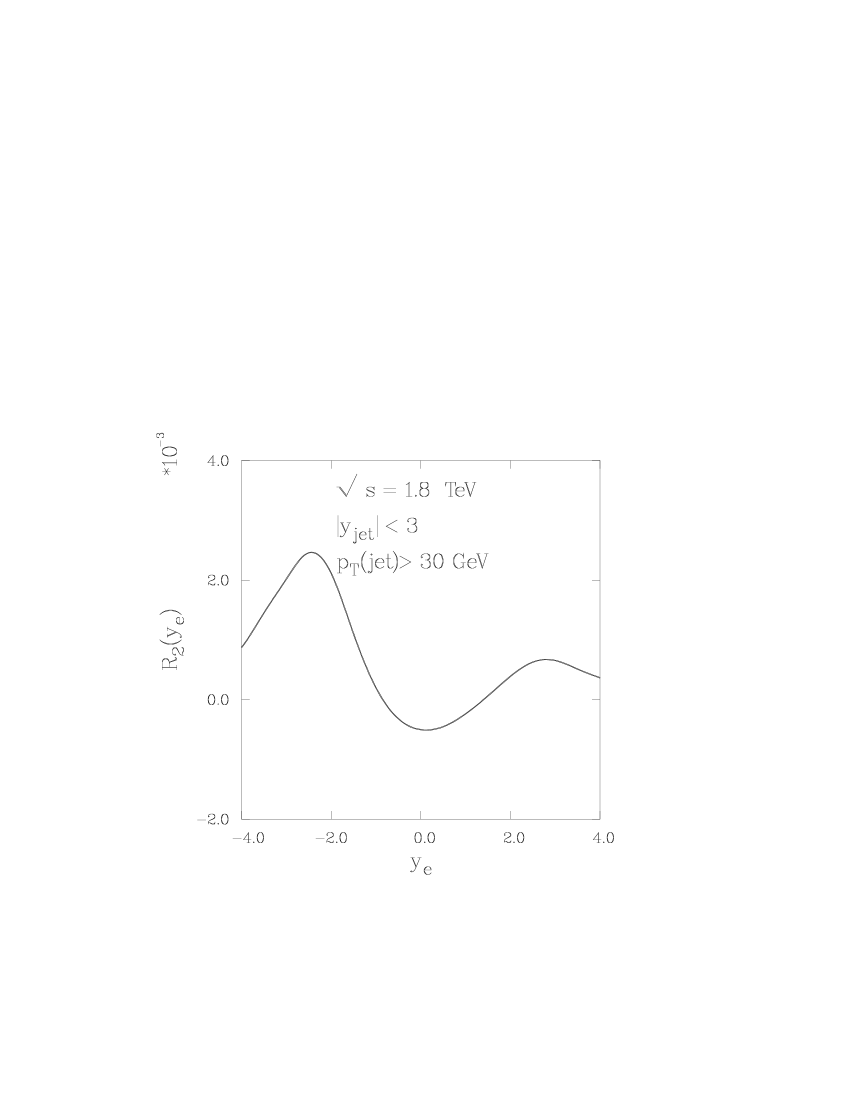
Figure 5: ${\cal CP}$ violating asymmetry in the lepton rapidity distributions as defined in Eq. 16. We used $\Lambda=1$ TeV and Im $\kappa=1$ in Eq. 18

We show in Figure 6 the distributions of the $A^{\pm}$ correlations with respect to the lepton transverse momentum. The ${\cal CP}$ violating nature of the interaction is reflected in the fact that the two distributions have opposite signs. Normalizing as in Eq.16 we present $R_{3}(p_{Te})$ in Figure 7.

Figure 6: Asymmetries $dA^{-}/dp_{Te}$ (solid line) and $dA^{+}/dp_{Te}$ (dotted line) normalized to the lowest order Standard Model cross section $\sigma(p\overline{p}\rightarrow e^{\pm}\nu{\rm jet})$

The rise in the asymmetry for large values of $p_{Te}$ is due to the decrease in the standard model distribution $d\sigma/dp_{Te}$ which is peaked around $M_{W}/2$. This increase in the asymmetry is thus accompanied by a decrease in the total number of events.

Figure 7: ${\cal CP}$ violating asymmetry in the lepton transverse momentum distributions as defined in Eq. 16. We used $\Lambda=1$ TeV and Im $\kappa=1$ in Eq. 18.

4 Conclusions

We have constructed several ${\cal CP}$-odd asymmetries that can be used to search for ${\cal CP}$ violation in $W^{\pm}+(0,1)~{}{\rm jet}$ events in $p\overline{p}$ colliders. We have estimated the contributions to these asymmetries from some simple ${\cal CP}$ violating effective operators that respect the symmetries of the Standard Model. Assuming that the scale of the new physics responsible for these operators is 1 TeV, we find that it is possible to search for ${\cal CP}$ violation at the Tevatron with as few as $10^{6}$ events. Similar observables can be constructed for other processes such as $p\overline{p}\rightarrow W^{\pm}\gamma$.

Acknowledgements The work of G.V. was supported in part by a DOE OJI award under contract number DEFG0292ER40730. G. V. thanks the theory group at BNL for their hospitality while part of this work was performed. We are grateful to S. Errede, T. Han, J. Hauptman and S. Willenbrock for helpful discussions.

References

- [1] R.K. Ellis, G. Martinelli, and R. Petronzio, Nucl. Phys. B211 106 (1983); P. Arnold and M. Reno, Nucl. Phys. B319 37 (1989), Erratum, Nucl. Phys. B330 284 (1990); P. Arnold, R.K. Ellis, and M.H. Reno, Phys. Rev. D40 912 (1989); R. Gonsalves, J. Pawlowski, and C.-F. Wai, Phys. Rev. D40 2245 (1989); W. Giele et. al., In Research Directions for the Decade, Snowmass 1990, World Scientific, 137 (1990)
- [2] P. Arnold and R. Kauffman, Nucl. Phys. B349 381 (1991) .
- [3] R. Barbieri, A. Georges and P. Le Doussal, Z. Phys. C32 (1986) 437.
- [4] J. Bernabeu, A. Santamaria and M. B. Gavela, Phys. Rev. Lett. 57 1514 (1986); W. S. Hou at. al., Phys. Rev. Lett. 57 1406 (1986).
- [5] A. Brandenburg, J. Ma, and O. Nachtmann, Z. Phys. C55 (1992) 115.
- [6] W. Buchmüller and D. Wyler, Nucl. Phys. B268 621 (1986).
- [7] C. Burgess and J. Robinson, in BNL Summer Study on CP Violation, (World Scientific, Singapore,1991), ed. S. Dawson and A. Soni.
- [8] R. D. Peccei and X. Zhang, Nucl. Phys. B337 269 (1990).
- [9] For a list of references see S. Rindani, in Workshop on High Energy Particle Physics III, (Madras, India, Jan 10-22, 1994), hep-ph/9411398; D. Chang, W. Y. Keung and I. Phillips, Phys. Rev. D48 4045 (1993)
- [10] A. Brandenburg, J. Ma, R. Munch, and O. Nachtmann, Z. Phys. C51 (1991) 225
- [11] F. Abe et al, CDF Collaboration, Phys. Rev. Lett. 74 850 (1995).
- [12] M. Atiya et. al., Phys. Rev. Lett. 70 2521 (1993).
- [13] J. F. Donoghue and G. Valencia, Phys. Rev. Lett. 58 451 (1987).
- [14] K. Hagiwara, K. Hikasa and N. Kai, Phys. Rev. Lett. 52 1076 (1984).