LBL-37014

Summary talk: Gauge Boson Self Interactions

Ian Hinchliffe

Theoretical Physics Group
Lawrence Berkeley Laboratory
University of California
Berkeley, California 94720

A review is given of the theoretical expectations of the self couplings of gauge bosons and of the present experimental information on the couplings. The possibilities for future measurements are also discussed.

Disclaimer

This document was prepared as an account of work sponsored by the United States Government. While this document is believed to contain correct information, neither the United States Government nor any agency thereof, nor The Regents of the University of California, nor any of their employees, makes any warranty, express or implied, or assumes any legal liability or responsibility for the accuracy, completeness, or usefulness of any information, apparatus, product, or process disclosed, or represents that its use would not infringe privately owned rights. Reference herein to any specific commercial products process, or service by its trade name, trademark, manufacturer, or otherwise, does not necessarily constitute or imply its endorsement, recommendation, or favoring by the United States Government or any agency thereof, or The Regents of the University of California. The views and opinions of authors expressed herein do not necessarily state or reflect those of the United States Government or any agency thereof, or The Regents of the University of California.

The electro-weak gauge bosons in the standard model of electroweak interactions interact with each other in a way that is fully described by the model. Deviations from the prescribed form cause the model to be non-renormalizable or, equivalently, to violate unitarity in high energy scattering [1]. In this review talk, I shall present a personal perspective on the determination of, and expectations for, these couplings. I shall discuss the form of the deviations from the standard model and how they are parameterized and then discuss the expectations for the deviations in extensions to the standard model. I will review the current experimental information and the possible impact of future experiments.

Deviations from the standard model must be parameterized in some way that will still allow predictions for experimental quantities to be made. It is convenient to begin with the general form of the $WWV$ coupling where $V$ is either a $Z$ boson or a photon [2].

$$L/(ig_{v}) = (W_{\mu\nu}^{a\dagger}W^{a\mu}-W_{\mu}^{a\dagger}W^{a\mu}_{\nu})V^{\nu}g_{1}^{V}+\kappa_{V}W_{\mu}^{a\dagger}W^{a}_{\nu}V^{\mu\nu}$$ (1)

$$+ \widetilde{\kappa_{V}}W_{\mu}^{a\dagger}W^{a}_{\nu}V_{\alpha\beta}\epsilon^{\mu\nu\alpha\beta}+\frac{\lambda_{V}}{M_{W}^{2}}W_{\rho\mu}^{a\dagger}W^{a\mu_{\nu}}V^{\rho\nu}-ig_{5}^{V}\epsilon^{\mu\nu\rho\sigma}(W_{\mu}^{a\dagger}\stackrel{{\scriptstyle\leftrightarrow}}{{\partial_{\rho}}}W_{\nu}^{a\dagger})V_{\sigma}$$

$$+ \frac{\widetilde{\lambda_{V}}}{M_{W}^{2}}W_{\rho\mu}^{a\dagger}W^{a\mu}_{\nu}V_{\alpha\beta}\epsilon^{\rho\nu\alpha\beta}+ig_{4}^{V}W_{\mu}^{a\dagger}W^{a}_{\nu}(\partial^{\mu}V^{\nu}+\partial^{\nu}V^{\mu})$$

$W^{a}_{\mu}$ ($W^{a}_{\mu\nu}$) represents the $W$ boson field (field strength) and $V_{\mu}$ (or $V_{\mu\nu}$) is that of the photon ($\gamma$) or $Z$ boson. The $SU(2)$ index $a$ will be dropped in what follows. Electromagnetic gauge invariance implies that $g_{5}^{\gamma}=g_{4}^{\gamma}=0$. In the standard model, $\lambda_{Z}=\lambda_{\gamma}=g_{5}^{\gamma}=g_{5}^{Z}=g_{4}^{A}=g_{4}^{Z}=\widetilde{\kappa_{V}}=\widetilde{\lambda_{V}}=0$, $\kappa_{Z}=\kappa_{\gamma}=g_{1}^{Z}=g_{1}^{\gamma}=1$, $g_{Z}=e\cot\theta_{W}$ and $g_{\gamma}=e$. Radiative corrections can induce small changes in these values at higher order in perturbation theory. The terms $\widetilde{\kappa},\widetilde{\lambda}$ and $g_{4}$ violate CP and are also zero at one loop in the standard model. Experimental constraints are often quoted in terms of $\lambda$ and $\Delta\kappa=\kappa-1$ which parameterize deviations from the standard model. The other possible self couplings are $ZZZ$, $ZZ\gamma$ and $Z\gamma\gamma$. In the standard model these are zero. They are severely constrained by electromagnetic gauge invariance and Bose symmetry and must vanish if all of the particles are on mass shell [2, 3]. I will phrase most of the following discussion in terms of $\kappa_{\gamma}$ and $\lambda_{\gamma}$ assuming that all the other couplings have the form given by the standard model. The arguments provided below can be extended to the other cases straightforwardly.

The standard, $SU(2)\times U(1)$ model, of electro-weak corrections has now been tested at the quantum (1-loop) level in experiments at LEP, SLC and elsewhere[4, 5]. In these radiative corrections, the gauge boson self interactions can appear in loop corrections to the $W$, $Z$ and photon propagators. If all loops involving gauge boson self interactions are ignored, the agreement between theory and experiment is less good [6, 7]. Direct determination of these self interactions comes from direct observation of gauge boson pairs at the Tevatron or, eventually, at LEPII.

Extensions to the standard model can produce values of the parameters in Equation 1 that deviate from the standard model form. I will assume that whatever extensions exist, they must satisfy $SU(2)\times U(1)$ gauge invariance. A model that does not do this will be difficult to reconcile with current data. It is convenient to distinguish two types of extensions to the standard model. First, there are models that, like the standard model, are renormalizable. In this case a finite number of new parameters is sufficient to fully describe the theory. Supersymmetric extensions of the standard model usually fall into this class. In models of this type the parameters in Equation 1 are modified by radiative (loop) corrections from the standard model values.

Second there are non-renormalizable theories. Such models have a mass scale $\Lambda$ that appears in the coefficient of the higher dimension operators. For experiments that probe energy scales ($E$) less than $\Lambda$, the effects of these operators are suppressed by powers of $(E/\Lambda)$. Although, such models contain, in principle, an infinite number of parameters, only a few of these will be relevant for experiment since the suppression will render the effects of most of them unobservable. The theory can then be regarded as an effective theory valid for $E<\Lambda$. At energies above $\Lambda$, the theory is replaced by a more fundamental one and the terms in the effective theory are computable in terms of the parameters of the more fundamental theory. This notion of an effective theory is a very useful one since it may be possible to severely constrain its form without knowing the full dynamics of the fundamental theory [9]. The best example of this type is the theory that describes the interaction of pions with each other at low energy. Introducing $U=exp(i\overline{\sigma}\hskip-2.84544pt\cdot\hskip-2.84544pt\overline{\pi}/f_{\pi})$, where the vector $\overline{\pi}$ represents the $\pi^{\pm},\pi^{0}$, the interactions are given by

$$tr(\partial_{\mu}U^{\dagger}\partial_{\mu}U)+O(\frac{1}{4\pi f_{\pi}})^{2}$$ (2)

This Lagrangian well describes QCD, i.e. the dynamics of $\pi-\pi$ scattering, on energy scales less than a few hundred MeV. At higher energies the full dynamics of (non-perturbative) QCD, including the details or resonances is needed to fully describe the scattering. The low energy Lagrangian is determined by the symmetries of low energy QCD, i.e. the fact that the pions are the Goldstone bosons of spontaneously broken chiral symmetry.

If there is new dynamics on a mass scale of a few TeV, such as is the case in technicolor[10] models or models where there are strong interactions between longitudinally polarized $W$ and $Z$ bosons at high energy[11], the effects of this dynamics can be parameterized by adding terms to the standard model Lagrangian[12]. These form of these terms is dictated by the requirement that they must not produce any effects that would invalidate the various standard model tests and they must be invariant under $SU(2)\times U(1)$. The form of the operators depends upon the particle content of the low energy effective theory. The theory must contain the quarks, leptons and gauge bosons; it may or may not contain Higgs scalars. If we assume that there are no light Higgs scalars then one can write 12 CP invariant operators of dimension 4 [13] or less. This lagrangian can be written as a gauged chiral model. In addition to the quark and lepton fields and the gauge boson fields, there is a field $\Sigma=exp(i\pi^{a}\tau^{a}/v)$ with $v=246$ GeV. The field $\pi^{a}$ provides the longitudinal degrees of freedom for the massive $W$ and $Z$ bosons. The kinetic energy for the gauge bosons is given by

$$\frac{v^{2}}{4}tr(D_{\mu}\Sigma^{\dagger}D^{\mu}\Sigma)-\frac{1}{2}W_{\mu\nu}W^{\mu\nu}-\frac{1}{2}B_{\mu\nu}B^{\mu\nu}$$ (3)

Here field $B_{\nu\mu}$ ($W_{\mu\nu}$) is the field strength of the $U(1)$ ($SU(2)$) part of the standard model. These terms also give the mass for the $W$ and $Z$ bosons and the photon. I will consider the effects of two of the additional operators

$$L_{1} =- \frac{v^{2}}{\Lambda^{2}}2ig\beta_{1}tr(W_{\mu\nu}D^{\mu}\Sigma^{\dagger}D^{\nu}\Sigma)$$

$$L_{2} = \frac{v^{2}}{\Lambda^{2}}g^{2}\tan\theta_{W}\beta_{2}(\Sigma B_{\mu\nu}\Sigma^{\dagger}W^{\mu\nu})$$ (4)

These give a contribution to $\kappa_{\gamma}$

$$\Delta\kappa_{\gamma} = \frac{v^{2}}{\Lambda^{2}}g^{2}(\beta_{1}-\beta_{2})$$

$$\lambda_{\gamma} = 0$$ (5)

However the term $L_{2}$ also contributes to the two point function of the gauge bosons and is therefore constrained by measurements at LEP and elsewhere as I will now discuss.

Recall how tests of the standard model are carried out. The model is fully described in terms of a set of parameters which can be taken, to be the Fermi constant $G_{F}$, the fine structure constant $\alpha_{em}$, the mass of the $Z$, the Higgs mass and the masses of the quarks and leptons. Taking these values as input, one computes the expected value of some experimentally observable quantity such as the cross section of $\nu-e$ scattering. This expected quantity has some error $\delta_{theory}$, that arises from the uncertainties in the parameters and residual uncertainty arising from the the calculation having been carried out to some order in perturbation theory. This is then compared with an experimental measurement which has an error $\delta_{expt}$. If the theory and experiment agree, the model is the tested with an accuracy that is the larger of $\delta_{theory}$ and $\delta_{expt}$. A failure of the model is revealed when there are experimental results that disagree with theory by more than the larger of $\delta_{theory}$ and $\delta_{expt}$. In a variant of the standard model, extra parameters appear and the values of these parameters can be adjusted to accommodate experimental values that the standard model fails to predict correctly.

The parameters appearing in equation 1 need to be related to physical quantities so that their values can be extracted from data. The general form of the $WWV$ vertex for bosons of momenta $p_{1}$, $p_{2}$ and $p_{3}$ and polarization tensors $\epsilon_{1}^{\mu}$, $\epsilon_{2}^{\nu}$ and $\epsilon_{3}^{\alpha}$ depends upon the invariant mass of the three bosons viz. $\Gamma^{\mu\nu\alpha}(p_{1}^{2},p_{2}^{2},p_{3}^{2})$. In the case of the $WW\gamma$ vertex, there is a physical point where all of the particles are on mass shell (static limit) i.e. $\Gamma^{\mu\nu\alpha}(M_{W}^{2},M_{W}^{2},0)$. At this point the quantities appearing in equation 1 are related to physical properties of the $W$ boson; $\kappa_{\gamma}$ and $\lambda_{\gamma}$ to the electric quadrapole moment ($Q$) and magnetic dipole moment ($\mu$) of the $W$.

$$\mu = \frac{e}{2M_{W}}(1+\kappa_{\gamma}+\lambda_{\gamma})$$ (6)

$$Q = -\frac{e}{M_{W}^{2}}(\kappa_{\gamma}-\lambda_{\gamma})$$ (7)

However these static quantities are not sufficient to describe the general properties of $\Gamma^{\mu\nu\alpha}(p_{1}^{2},p_{2}^{2},p_{3}^{2})$.

Consider the process $q\overline{q}\to W\gamma$; I will assume for simplicity that all of the parameters in the $WW\gamma$ vertex have the standard form except for $\kappa_{\gamma}$ and $\lambda_{\gamma}$.

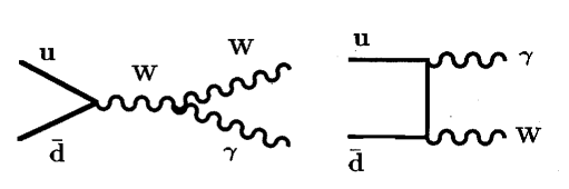
Figure 1: Feynman diagrams showing the process $q\overline{q}\to W\gamma$

There is a contribution for the Feynman diagram shown in figure 1 which depends on $\Gamma^{\mu\nu\alpha}(s,M_{W}^{2},0)$ where $\sqrt{s}$ is the center of mass energy of the quark antiquark system. If $\kappa_{\gamma}$ and $\lambda_{\gamma}$ are taken to be constants, then this will result in a scattering amplitude of the form

$$A\sim a+b\sqrt{s}(\kappa_{\gamma}-1+\lambda_{\gamma})+cs\lambda_{\gamma}$$ (9)

where $a$, $b$ and $c$ are independent of the center of mass energy ($\sqrt{s}$). This amplitude grows with $s$ unless $\kappa_{\gamma}$ and $\lambda_{\gamma}$ have the standard model values of $1$ and $0$ respectively. This growth is a general feature of anomalous couplings. It is immediately clear that the sensitivity of an experiment to the anomalous couplings increases with the energy of the experiment and that a high energy experiment is more sensitive to $\lambda_{\gamma}$ than to $\kappa_{\gamma}-1$. Hence an $e^{+}e^{-}\to W^{+}W^{-}$ measurement at $\sqrt{s}\sim 500$ GeV can constrain $\lambda_{\gamma}$ and $\kappa_{\gamma}-1$ much more precisely than a measurement with comparable statistical power at $\sqrt{s}\sim 190$ GeV. Similarly in a hadron collider, the greatest sensitivity arises from the (few) events of largest energy.

This problem of unitarity violations can be avoided phenomenologically by the introduction of form factors [14] to damp the growth at large $s$ i.e.  $\lambda_{\gamma}\to\lambda_{\gamma}/(1+s/\Lambda^{2})^{n_{1}}$ and $(\kappa_{\gamma}-1)\to(\kappa_{\gamma}-1)/(1+s/\Lambda^{2})^{n_{2}}$ with $n_{1},n_{2}\geq 1$. It is conventional to use a dipole form factor, i.e. $n_{2}=n_{1}=2$. An experiment measuring the $W\gamma$ production cross section can set a limit on $\Delta\kappa_{\gamma}$ and $\lambda_{\gamma}$ given a value of $n_{1}$, $n_{2}$, and $\Lambda$. Note that for a given choice of $n_{1}$, $n_{2}$, and $\Lambda$, unitarity alone bounds $\lambda_{\gamma}$ and $\kappa_{\gamma}-1$. For $n_{1}=n_{2}=2$, this bound is [15]

$$\left|\kappa_{\gamma}-1\right| < 7.4\hbox{ TeV}^{2}/\Lambda^{2}$$

$$\left|\lambda_{\gamma}\right| < 4.0\hbox{ TeV}^{2}/\Lambda^{2}$$ (10)

An experiment that is not sensitive to values below these is not relevant.

Generally $\Gamma^{\mu\nu\alpha}(p_{1}^{2},p_{2}^{2},p_{3}^{2})$ is not gauge invariant when computed beyond leading order in perturbation theory. This is directly related to the fact that it is not a physical quantity. As discussed in reference [16], it is possible to define a gauge invariant form by including some pieces of other corrections that would contribute at the same order in perturbation theory to a physical process. In the example of $q\overline{q}\to W\gamma$, a contribution of this type is shown in figure 2.

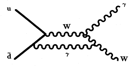
Figure 2: An example of contribution to $q\overline{q}\to W\gamma$ which must be included along with the 1 loop corrections to the $WW\gamma$ vertex appearing in Figure 1

It is convenient to quote the values of the physical quantities $\lambda_{\gamma}$ and $\Delta\kappa_{\gamma}$ at the static limit as a measure of the expected size of the higher order corrections.

What values of anomalous couplings are to be expected in the standard model and its possible extensions? In the standard model the natural size of $\kappa_{\gamma}-1$ and $\lambda_{\gamma}$ is $\alpha_{em}/\pi$ [17]. For a top quark mass of 150 GeV and a Higgs mass of 100 GeV, $\lambda_{\gamma}=0.006$ and $\kappa_{\gamma}+\lambda_{\gamma}-1=-0.0003$[18]. In the supersymmetric model the size of the corrections depends upon the masses of the supersymmetric particles. Note that the masses assumed must be consistent with other experimental constraints. For most of the values of the parameters, $\lambda_{\gamma}$ is about 60% of its value in the standard model and $\kappa_{\gamma}+\lambda_{\gamma}-1$ is about 5 times larger than its standard model value.

In extensions to the standard model where operators of the type in equation 4 are present, we need to estimate the size of $\beta_{1},\beta_{2}$, and $\Lambda$. Using the scale of new physics $\Lambda$ to be 1 TeV we might expect $\delta\kappa_{\gamma}$ to be as large as 0.05 if $\beta_{1}\sim\beta_{2}\sim 1$ as would be expected if the new physics at scale $\Lambda$ is strongly coupled. Other estimates yield values smaller than these [12]. The term $L_{2}$ in equation 4 contributes to the gauge boson two point functions and in particular to the Peskin-Takeuchi [19] $S$ parameter. Using the data from LEP, the constraint $\left|\beta_{2}\right|\raisebox{-1.72218pt}{\hbox to0.0pt{$\sim$\hss}}\raisebox{1.72218pt}{$<$}0.5$[20] is obtained (again I have taken $\Lambda=1$ TeV). Hence the contribution of $L_{2}$, to $\Delta\kappa_{\gamma}$ is restricted to be less than 0.013. The term $L_{1}$ is not directly constrained by LEP data. However since both $\beta_{1}$ and $\beta_{2}$ arise from the same (unknown) physics, it is to be expected that they will be of the same order of magnitude.

There have been observations of $W\gamma$, $Z\gamma$, $WW$ and $WZ$ final states at the Tevatron collider by both CDF[21] and D0[22] that are reviewed at this meeting [23, 24] The former constrains the $WW\gamma$ vertex while the latter constrains the $ZZ\gamma$ and $Z\gamma\gamma$ vertices and the last constrain $WWZ$ and $WW\gamma$ vertices. The limits on $\kappa_{\gamma}$ and $\lambda_{\gamma}$ arising from observation of $W\gamma$ final states are shown in Figure 3. These limits use dipole form factors ($n_{1}=n_{2}=2$) with $\Lambda=1.5$ TeV. The limits are essentially unchanged if $\Lambda=1$ TeV. The unitarity limits for $\Lambda=1.5$ TeV are larger than the experimental constraints (see figure 3).

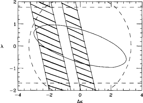
Figure 3: The limits on $\Delta\kappa_{\gamma}$ and $\lambda_{\gamma}$ from the D0 experiment (the area inside the oval region is allowed region) [22]. The limits from CDF are similar [21]. Also shown is the allowed region from the observation of $b\to s\gamma$ (the hatched area) from CLEO[28]. The limits are shown at 95% confidence. The area outside the dashed circle is excluded by unitarity for the process $q\overline{q}\to W^{+}W^{-}$ with $n_{1}=n_{2}=2$ and $\Lambda=1.5$ TeV. The regions at the top and bottom of the figure bounded by the dashed horizontal lines are excluded by unitarity in $q\overline{q}\to W_{\gamma}$

The limits on $\kappa_{Z}$ and $\lambda_{Z}$ arising from the observation of $WW$ and $WZ$ final states is similar to those on $\kappa_{\gamma}$ and $\lambda_{\gamma}$ [21]. In the case of the $ZZ\gamma$ and $Z\gamma\gamma$ vertices, the limits are more sensitive to the assumed form factor behaviour of the vertices [3]. This is due to the form of the vertex function, $\Gamma^{\mu\nu\alpha}(p_{1}^{2},p_{2}^{2},p_{3}^{2})$, which must vanish when the particles are all on mass shell and therefore has powers of energy in the numerator. The form factors then introduced to prevent a unitarity violation must have $n\geq 3$. Constraints have also been placed on the $ZZ\gamma$ couplings by searching for events at LEP of the form $Z\to\gamma Z^{*}(\to\nu\overline{\nu})$ [27]. These limits are comparable to those from CDF.

Note that the limits depend upon the ability to predict the event rates given the gauge boson self couplings requires an understanding of the QCD production process. This process is computed at next to leading order in $\alpha_{strong}$ and the resulting uncertainty should quite small [25]. The angular distribution of the process $q\overline{q}\to W\gamma$ has a zero at a particular value of the scattering angle [26]. This zero is not preserved by the higher order QCD corrections.

The decay of a B meson to a photon and a strange meson, proceeds via loop effects. One relevant graph is given in Figure 4, where the $WW\gamma$ vertex is present.

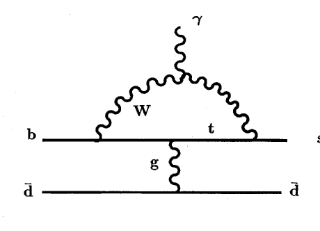
Figure 4: A contribution to the process $B\to K\gamma$

The experimental observation of this process [28] enables one to constrain $\kappa_{\gamma}$ and $\lambda_{\gamma}$ [29]. The constraint is shown on Figure 3. Note that the constraint is less direct than that of CDF and D0. The interference between the graph shown in figure 4 and other graphs such as the one where the photon is radiated off the top quark, results in the odd shape for the allowed region. If there were other diagrams that could contribute to $b\to s\gamma$, such as would occur in a supersymmetric model, the constraint becomes a coupled limit involving the couplings of other particles [30].

I will end with a discussion of the prospects for future measurements. LEP II will be able to measure the $Z\gamma$ and $WW$ and possibly the $ZZ$ final state. Consequently it will probe the $WW\gamma$, $ZZ\gamma$, $Z\gamma\gamma$ and $WWZ$ vertices. In the case of $WW\gamma$, the sensitivity of order 0.3 (0.5) to both $\lambda$ and $\Delta\kappa$ at $\sqrt{s}=192(176)$ GeV [32]. This is approximately three times better than the current limits from the Tevatron. However these limits are based on $\sim 15$ pb^-1 of data. They will improve by the end of the current when $\sim 100$ pb^-1 will be available. If it is then possible to combine the CDF and D0 limits, they should fall by a factor of three or so. It seems reasonable to conclude therefore that any improvement that LEP II can provide over the Tevatron will be small.

There has been much discussion in the literature [20, 31] and at this meeting of the extent to which the precision measurements of LEP imply that LEPII cannot see any effects of anomalous couplings. In order to address this question, possible models that differ from the standard model must be constructed so that they are consistent with LEP data and predictions for anomalous couplings or measurements at LEPII made. As discussed above, the LEP data constrain $\beta_{2}$ of Equation 4 sufficiently that the contribution of $L_{2}$ to anomalous couplings is too small to be seen at LEPII. The “natural” values of $\beta_{2}$ and $\beta_{1}$ should be roughly equal. In this case it is unlikely that LEPII (or the Tevatron) will see a positive effect. However, it might happen that $\beta_{1}>>\beta_{2}$. In QED, one can estimate the natural size of a process by assuming that the coefficient of the appropriate power of $\alpha_{em}/\pi$ is order one. Large coefficients such as $\pi^{2}$ that appears in the radiative corrections to Coulomb scattering [33] as well as ones that are less than one, such as the order $\alpha\pi$ correction to $g-2$ of the electron do occur.

The sensitivities of experiments discussed above are very far from the deviations from the standard model that can reasonably be expected. Experiments at LHC [34, 35] have greater sensitivity because of their greater energy. ATLAS expects a sensitivity of order $\Delta\kappa_{\gamma}\sim 0.04$ $\lambda_{\gamma}\sim 0.0025$ which is approaching values that are theoretically interesting[35]. An $e^{+}e^{-}$ collider with more energy than LEP will be more sensitive; at $\sqrt{s}=500$ GeV (1.5 TeV) the sensitivities are $\lambda_{\gamma}$ and $\Delta\kappa_{\gamma}$ are $\sim 0.01$ ($\sim 0.002$) [36].

I am grateful to the members of the organizing committee, U. Baur, S. Errede and T. Müller for their work in making this conference such a success. The work was supported by the Director, Office of Energy Research, Office of High Energy Physics, Division of High Energy Physics of the U.S. Department of Energy under Contract DE–AC03–76SF00098. Accordingly, the U.S. Government retains a nonexclusive, royalty-free license to publish or reproduce the published form of this contribution, or allow others to do so, for U.S. Government purposes.

References

- [1] H.H. Llewellyn Smith, Phys. Lett. 46B, 233 (1973); S.D. Joglekar, Ann. Phys. (NY) 83, 427 (1974); J.M. Cornwall, D.N. Levin and G. Tiktopolous, Phys. Rev. Lett. 30, 1268 (1973).
- [2] K. Hagiwara, et al. Nucl. Phys. B282, 253 (1987).
- [3] U. Baur and E. Berger, Phys. Rev. D47, 4889 (1993).
- [4] D. Schaile these proceedings and CERN-PPE-94-162.
- [5] T. Takeuchi, these proceedings.
- [6] P. Gambini and A. Sirlin Phys. Rev. Lett. 73, 621 (1994).
- [7] K. Hagiwara and S. Matsumoto, KEK-TH-375 (1994) and these proceedings.
- [8] S. Willenbrock, these proceeedings.
- [9] For a review, see e.g.H. Georgi, Ann. Rev. Nucl. and Part. Sci. 43, 209 (1993).
- [10] For a review see, for example, K.D. Lane, BUHEP-94-26 (1994) and references therein.
- [11] M. Chanowitz, in Perspectives on High Energy Physics, Ed. G. Kane, World Scientific Publishing (1992).
- [12] C. Arst, M.N. Einhorn and J. Wudka, Nucl. Phys. B433, 41 (1995).
- [13] A Longhitano Nucl. Phys. B188, 118 (1981); T. Appelquist and C. Bernard, Phys. Rev. D22, 200 (1980).
- [14] U. Baur and D. Zeppenfeld, Nucl. Phys. B308, 127 (1988).
- [15] U. Baur and D. Zeppenfeld, Phys. Lett. 201B, 383 (1988).
- [16] J.M. Cornwall, in Deeper Pathways in High Energy Physics, ed. B. Kursunoglu, A. Perlmutter and L. Scott, Plenum Press (1977), G. Degrassi and A. Sirlin Phys. Rev. D46, 3104 (1992).
- [17] W.A. Bardeen, R. Gastmans and B. Lautrup Nucl. Phys. B46, 319 (1982); K.J. Kim and Y.S. Tsai, Phys. Rev. D12, 3972 (1975).
- [18] E.N. Argyres et al., Nucl. Phys. B391, 23 (1993); J. Papavassiliou and K. Philoppides, Phys. Rev. D48, 4255 (1993).
- [19] M. Peskin and T. Takeuchi, Phys. Rev. Lett. 65, 964 (1990).
- [20] S. Dawson and G. Valencia, BNL-60949 (1994).
- [21] F. Abe, et al. FNAL-PUB-95/036-E, Phys. Rev. Letters (submitted), FNAL-PUB-94/236-E Phys. Rev. Letters (submitted).
- [22] S. Abachi et al., Phys. Rev. Letters (submitted), J. Ellison in Proc. of 1994 DPF Meeting, Albuquerque, NM.
- [23] H. Aihara, these proceedings.
- [24] T. Fuess, these proceedings.
- [25] J. Ohnemus, these proceedings; U. Baur, T. Han, J. Ohnemus FSU-HEP-941010 (1994).
- [26] R.W. Brown, D. Sadhev and K.O. Mikaelian, Phys. Rev. D20, 1164 (1999); R.W. Brown, these proceedings.
- [27] P. Mattig, these proceedings; O. Adrianni et al., Phys. Lett. B297, 469 (1992); M. Acciarri, et al. Phys. Lett. B345, 609 (1995).
- [28] M.S. Alam et al., CLNS-94-1314 (1994); S. Playfer, these proceedings.
- [29] S. Chia Phys. Lett. B240, 467 (1990); K. Peterson Phys. Lett. B282, 207 (1992); T. Rizzo Phys. Lett. B315, 471 (1993) and X. He and B. McKellar Phys. Lett. B320, 165 (1994).
- [30] J. Hewett, SLAC-PUB 6521, Presented at SLAC Summer Inst. on Particle Physics, SLAC, Jul 6 - Aug 6, 1993.
- [31] P. Hernandez and F.J. Vegas, Phys. Lett. B307, 116 (1993); A. De Rujula, M.B. Gavela, P. Hernandez, and E. Masso Nucl. Phys. B384, 3 (1992); P.Hernandez, these proceedings.
- [32] Talks by G,. Gounaris and J.L. Knuer, LEPII workshop Jan 1995; R.L. Sekulin Phys. Lett. B338, 369 (1994); J. Hansen ALEPH-95-004.
- [33] J. Schwinger, Phys. Rev. 75, 1912 (1949).
- [34] J. Womersley, these proceedings; ; CMS technical proposal CERN/LHCC/94-38.
- [35] ATLAS technical proposal CERN/LHCC/94-43.
- [36] T. Barklow, these proceedings, SLAC-PUB-6618 (1994).