CERN–TH/95–65/R UM–TH–95–07/R hep-ph/9503492 March 1995

Resummation of Running Coupling Effects in
Semileptonic B Meson Decays and Extraction of $|V_{cb}|$

Patricia Ball¹, M. Beneke² and V.M. Braun³

¹CERN, Theory Division, CH–1211 Genève 23, Switzerland
²Randall Laboratory of Physics, University of Michigan, Ann Arbor, Michigan 48109, USA
³DESY, Notkestraße 85, D–22603 Hamburg, Germany

Abstract
We present a determination of $|V_{cb}|$ from semileptonic B decays that includes resummation of supposedly large perturbative corrections, originating from the running of the strong coupling. We argue that the low value of the BLM scale found previously for inclusive decays is a manifestation of the renormalon divergence of the perturbative series starting already in third order. A reliable determination of $|V_{cb}|$ from inclusive decays is possible if one either uses a short-distance b quark mass or eliminates all unphysical mass parameters in terms of measured observables, such that all infra-red contributions of order $1/m_{b}$ cancel explicitly. We find that using the $\overline{\rm MS}$ running mass significantly reduces the perturbative coefficients already in low orders. For a semileptonic branching ratio of $10.9\%$ we obtain $|V_{cb}|(\tau_{B}/1.50\,{\rm ps})^{1/2}=0.041\pm 0.002$ from inclusive decays, in good agreement with the value extracted from exclusive decays.

submitted to Phys. Rev. D

1 Introduction

The physics of heavy flavours has experienced a rapid development within the past few years, driven by new data that aim to test the Standard Model and to determine its fundamental parameters. In particular, semileptonic B decays for the moment provide the best possibility to determine the CKM matrix element $|V_{cb}|$. Two competing strategies, which both have received considerable attention, are the determination of $|V_{cb}|$ from the total inclusive semileptonic decay rate [1] and from the exclusive $B\to D^{*}l\bar{\nu}$ decays at the point of zero recoil [2]. In both cases the absence of $1/m_{b}$ corrections allows an accurate theoretical description. The decay rates can be calculated within perturbation theory up to terms of order $1/m_{b}^{2}$. Moreover, the $1/m^{2}_{b}$ corrections are estimated to be rather small ($\sim 5\%$). Thus, at present, the theoretical accuracy of the determination of $|V_{cb}|$ is to a large extent limited by a poor control over perturbative radiative corrections, which are only known to one-loop accuracy. An explicit calculation of the second order correction is a very hard enterprise already for $b\rightarrow u$ transitions and even more so for $b\rightarrow c$ transitions because of the c quark mass, whose numerical effect is very important, see [3, 4].

A process of major phenomenological interest is the total inclusive B meson decay rate with a c quark in the final state, which is calculable in perturbation theory as

$$\Gamma(B\to X_{c}e\bar{\nu})=\Gamma_{0}(a)\left[1-C_{F}\frac{\alpha_{s}}{\pi}g_{0}(a)+O(\alpha_{s}^{2})\right],$$ (1.1)

where $C_{F}=4/3$ and $a=(m_{c}/m_{b})^{2}$.

The tree-level decay rate, including the phase space factor $f_{1}(a)$, reads

$$\Gamma_{0}(a) = \frac{G_{F}^{2}m_{b}^{5}}{192\pi^{3}}f_{1}(a)\,,$$

$$f_{1}(a) = 1-8a+8a^{3}-a^{4}-12a^{2}\ln a,$$ (1.2)

and the function $g_{0}(a)$ is known in analytic form [5]. Here and below $m_{b}$ and $m_{c}$ denote pole masses. The perturbative expression in (1.1) should be complemented by non-perturbative corrections suppressed by powers of the heavy quark masses [6], and we will take these corrections into account in the final analysis. In the major part of the paper, however, we restrict ourselves to perturbation theory and estimate higher-order perturbative corrections to (1.1).

For the realistic value $m_{c}/m_{b}=0.3$, Luke, Savage and Wise [7] have given an estimate for the $\alpha_{s}^{2}$ correction in (1.1) as

$$1-1.67\frac{\alpha_{s}(m_{b})}{\pi}-15.1\left(\frac{\alpha_{s}}{\pi}\right)^{2}$$ (1.3)

where $\alpha_{s}$ is the $\overline{\rm MS}$ coupling. For $m_{c}/m_{b}\to 0$, i.e. for $b\to u$ decays, the estimated size of the second order correction is even more striking [7]:

$$1-2.41\frac{\alpha_{s}(m_{b})}{\pi}-28.7\left(\frac{\alpha_{s}}{\pi}\right)^{2}.$$ (1.4)

The coefficients in front of $\alpha_{s}^{2}$ were in both cases obtained by an explicit calculation of the diagrams corresponding to the insertion of a fermion loop into the gluon line in the leading-order virtual correction, as in Fig. 1(b), or the splitting of an emitted gluon into a light quark-antiquark pair, for the real emission. These contributions are proportional to the number of light fermion flavours and the above numerical estimates are obtained by restoring the full one-loop QCD $\beta$-function by the substitution $N_{f}\to N_{f}-33/2$.

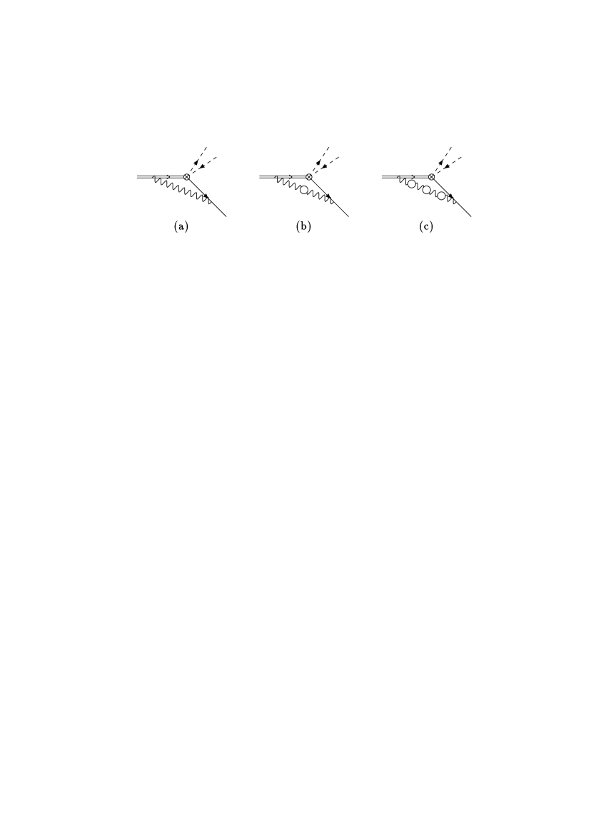
Figure 1: Generic radiative corrections for heavy-particle decays: (a) leading order, (b) with a fermion bubble insertion, and (c) with a chain of fermion bubbles. The broken lines represent the lepton pair produced in the decay.

This replacement assumes the hypothesis of BLM [8] that the dominating radiative corrections originate from the running of the strong coupling. The result of this procedure is usually expressed as a redefinition of the scale of the coupling in the leading-order correction that completely absorbs the second order correction. The magnitude of these corrections leads to very low BLM scales for semileptonic decays [7]:

$$\mu_{1}^{b\to u}=0.07m_{b},\quad\mu_{1}^{b\to c}=0.13m_{b},$$ (1.5)

with numerical values of order (350–650) MeV that are hardly acceptable. The authors of Ref. [7] interpreted their result as an indication that an accurate determination of $|V_{cb}|$ from inclusive decays requires knowledge of the exact second order correction and even those of higher order. In Ref. [9] the large two-loop correction was interpreted as a breakdown of perturbation theory which disfavours the inclusive approach to $|V_{cb}|$ in comparison to the exclusive one, for which large radiative corrections do not appear in the same approximation [9]. On the other hand, as noted in [10], the difference in the size of the $\alpha_{s}^{2}$ correction for inclusive and exclusive decays largely disappears, when the scale of the leading-order correction is chosen equally as $\sqrt{m_{c}m_{b}}$ in both cases. Still, the very fact of low BLM scales suggests the investigation of yet higher order radiative corrections.

It is this question we address in this paper. Our analysis extends the results of Ref. [7] for inclusive decays and repeats that of [11] for exclusive ones in that we resum the effects due to one-loop running of the strong coupling, but to all orders in perturbation theory. Thus, our investigation of higher order corrections assumes the dominance of vacuum polarization effects also in higher orders and we do not address the question whether knowledge of the exact two- (and higher) loop corrections as compared to the BLM approximation is important. The idea is that if higher order corrections are large at a certain scale, they are presumably dominated by running coupling effects and can thus be taken into account exactly, at least within the restriction to one-loop running. The remaining corrections are then small and therefore can only be accounted for by an exact calculation. Formally, we resum terms of the type $\alpha_{s}(\beta_{0}\alpha_{s})^{n}$, of which the correction found in [7, 9] is the first term with $n=1$. These can be traced by a calculation of contributions proportional to $N_{f}^{n}$ given by a chain of fermion loops as in Fig. 1(c). The leading-order BLM scales calculated in [7, 9] correspond to using the QCD coupling at some characteristic virtuality obtained by averaging $\ln k^{2}$, where $k$ is the gluon momentum, over the leading-order diagram. The resummation that we perform in this paper amounts to averaging with the one-loop running coupling $\alpha_{s}(k^{2})$ itself, rather than $\ln k^{2}$. We have developed a technique to implement this resummation in Refs. [12, 13] and refer the reader to these articles for all conceptual and technical issues that we do not repeat in the present application to semileptonic B decays.

We find that the large second order radiative correction to $b\to ue\bar{\nu}$ transitions calculated in [7] is in fact already close to the regime, where the series starts to diverge because of factorially growing coefficients. In our approximation (called ‘Naive Non-Abelianization’ in [12, 13]) the series in (1.4) is continued as

$$1-2.41\frac{\alpha_{s}}{\pi}\Bigg{\{}1+11.12\left(\frac{\alpha_{s}}{\pi}\right)+149.3\left(\frac{\alpha_{s}}{\pi}\right)^{2}+2319\left(\frac{\alpha_{s}}{\pi}\right)^{3}+42751\left(\frac{\alpha_{s}}{\pi}\right)^{4}+\ldots\Bigg{\}},$$ (1.6)

and with $\alpha_{s}(m_{b})=0.21$ one gets a non-convergent series of corrections to the decay rate already in low orders:

$$\Gamma(B\to X_{u}e\bar{\nu}) = \Gamma_{0}(0)\left\{1-2.41\frac{\alpha_{s}(m_{b})}{\pi}\Big{[}1+0.75+0.67+0.70+0.87+1.27+\ldots\Big{]}\right\}$$ (1.7)

$$= \Gamma_{0}(0)\left\{1-2.41\frac{\alpha_{s}(m_{b})}{\pi}\Big{[}2.31\pm 0.62\Big{]}\right\}$$

$$= (0.63\pm 0.10)\,\Gamma_{0}(0).$$

In attributing a numerical value to this divergent series we assume that it is asymptotic. Then one must truncate it at the minimal term and its value gives an estimate of the intrinsic limitation of the perturbative calculation, which cannot be reduced by computing higher orders.

For $b\to ue\bar{\nu}$ transitions the minimal term occurs at third order in $\alpha_{s}$ and its size is comparable to the second order correction. Numerically, it gives a 15% uncertainty for the total decay rate, not taking into account the uncertainty in the input parameters $\alpha_{s}$ and the quark masses. For $b\to ce\bar{\nu}$ transitions, in the same approximation of vacuum polarization dominance, we obtain

$$\Gamma(B\to X_{c}e\bar{\nu})=(0.77\pm 0.05)\,\Gamma_{0}(0.3)$$ (1.8)

with a 7% uncertainty. We also note that the uncertainties associated with the fixed-sign factorial divergence of perturbative expansions cannot be reduced by the use of a different renormalization scheme, or a change of scale in the coupling [14]. Thus, the change of scale suggested in Ref. [10], which decreases the second order coefficient, is ineffective already at the next order, because the reduction of coefficients is compensated by an increase of $\alpha_{s}$.

However, it would be premature to draw a pessimistic conclusion from the apparently bad behaviour of perturbative corrections. The large corrections displayed above originate from infra-red regions in the integration over loop momenta and produce an uncertainty parametrically of order $\Lambda_{\rm QCD}/m_{b}$. As it turns out, the importance of infra-red regions is solely due to the choice of an input parameter – the pole mass as renormalized mass parameter –, which is incompatible with the short-distance properties of the decay process. The series that relates the pole to the bare mass contains large finite renormalizations of infra-red origin. If these are made explicit – for example using the $\overline{\rm MS}$ renormalized mass – they cancel with the large corrections of infra-red origin present in the perturbative series for the decay width [15, 16].

The preference of the $\overline{\rm MS}$ (or another ‘short-distance’) mass might seem surprising and even counter-intuitive. After all, it is the pole mass that governs the (partonic) decay kinematics and it is the visualization of an almost on-shell (up to effects of order $\Lambda_{\rm QCD}$) b quark inside the meson that motivated the approximation of the meson decay by a free quark decay in the first place. But this picture also implies the existence of a static field (in the rest frame of the quark) around the heavy quark, which behaves as $1/r$ at short distances. Thus a contribution of order $\Lambda_{\rm QCD}$ to the self-energy of the quark is stored at large distances, $r\sim 1/\Lambda_{\rm QCD}$, of the order of the radius of the heavy-light meson. However, due to the Kinoshita-Lee-Nauenberg cancellations, in an inclusive decay of a heavy quark the decay vertex is localized to within a distance $1/m_{b}$ and the energy stored in the field at large distances $r\geq 1/\mu$ (where $m_{b}>\mu\geq\Lambda_{\rm QCD}$ is a factorization scale) cannot participate in the hard process, but is absorbed into a rearrangement of the colour field of the hadronizing spectator quark. This explains, loosely spoken, why a short-distance mass is more appropriate in the description of inclusive decays as a hard process. This reasoning assumes that the quark produced by the weak current is fast and does not apply to a massive quark produced with zero recoil (cf. Sec. 3.2).

Since ultimately any quark mass parameter is unphysical, the most transparent way to exhibit the infra-red cancellations would be to eliminate any mass parameter in terms of a suitable physical quantity, provided it is determined by short distances and does not import $1/m_{b}$ corrections (which rules out meson masses). However, as with the strong coupling constant, it is convenient to use a mass parameter for book-keeping purposes and as a numerical input parameter. It is only at this point that the $\overline{\rm MS}$ mass (or any other mass defined at short distances) is favoured over the pole mass, because it does not import infra-red effects.

In fact, the divergence of the series of radiative corrections to the decay rates is only one aspect of the problem with using the pole mass. Another aspect is that it cannot be accurately extracted from measurable quantities through perturbative expansions [15, 17].

To reinforce this point we imagine that we used pole masses as numerical input parameters, determined from another measurement. Then one would always find that the size of perturbative corrections does not allow a determination of the masses to an accuracy better than $\pm 100\,$MeV (we quote the estimate from [13]). Treating the uncertainty in the input parameters as uncorrelated with the uncertainty in the theoretical prediction for the radiative corrections to the B decay width, we obtain a $\pm$21% and $\pm$10% uncertainty for $B\to X_{u}e\bar{\nu}$ and $B\to X_{c}e\bar{\nu}$ decays, respectively. This translates into an irreducible theoretical uncertainty of $\pm$10% in $|V_{ub}|$ and $\pm$5% in $|V_{cb}|$. The $10\%$ uncertainty in $\Gamma(B\to X_{c}e\bar{\nu})$ is to be compared with the present experimental uncertainty of 12% of the branching ratio.

The calculation of decay rates with running masses has already been considered in [18] at the level of one-loop perturbative corrections. After resummation, we find that apart from the cancellation of infra-red contributions the perturbative coefficients are strongly reduced already in low orders. In particular, if the $\overline{\rm MS}$ running mass is used in the tree-level decay rate, the series of radiative corrections for $b\to ue\bar{\nu}$ decays becomes

$$1+4.25\frac{\alpha_{s}}{\pi}\Bigg{\{}1+8.99\left(\frac{\alpha_{s}}{\pi}\right)+35.15\left(\frac{\alpha_{s}}{\pi}\right)^{2}+241.1\left(\frac{\alpha_{s}}{\pi}\right)^{3}+1547\left(\frac{\alpha_{s}}{\pi}\right)^{4}+\ldots\Bigg{\}}.$$ (1.9)

Although the leading-order correction has increased (and changed sign), the higher-order coefficients are significantly reduced, so that with the same value of $\alpha_{s}$ as above we get the well convergent series

$$\Gamma(B\!\to\!X_{u}e\bar{\nu}) = \overline{\Gamma}_{0}(0)\left\{\!1+4.25\frac{\alpha_{s}(m_{b})}{\pi}\Big{[}1+0.604+0.159+0.073+0.032+0.022+\ldots\Big{]}\!\right\}$$ (1.10)

$$= \Gamma_{0}(0)\left\{1+4.25\frac{\alpha_{s}(m_{b})}{\pi}\Big{[}1.92\pm 0.01\Big{]}\right\}$$

with an uncertainty that is negligible compared to the uncertainty inherent in the restriction to vacuum polarization corrections.

It should be noted that anticipating the eventual cancellation of infra-red regions we can define the numerical value of the sum of radiative corrections even when it diverges, with some (ad hoc) prescription. Provided we use the same prescription to define the pole mass, and provided we know that the cancellation occurs, we can then simply delete nearly all large uncertainties. Thus, the calculation in the on-shell scheme (using pole masses) can be saved at the cost of introducing consistent non-perturbative prescriptions to define the pole mass and to sum the series of radiative corrections. We shall consider this (conceptually less appealing) possibility as well, and shall see that after resummation of $\beta_{0}^{n}\alpha_{s}^{n+1}$ corrections the decay rates calculated in the on-shell and $\overline{\rm MS}$ schemes are close to each other, provided the same short-distance mass is used as an input parameter. This supports a posteriori the assumption that the dominant higher order corrections are taken into account by vacuum polarization effects.

We conclude that the large corrections found in [7] do not endanger the accuracy of the theoretical treatment of inclusive decays. We do find, however, large corrections beyond second order in $\alpha_{s}$, in particular in the on-shell scheme, defined in the sense of the previous paragraph. We suggest that these corrections are more important than the $\alpha_{s}^{2}$ corrections left out by the restriction to the effects of running coupling. Although the accuracy of this restriction is not known and is certainly the main deficiency of our analysis, we believe that resummation of one-loop running effects provides a fair estimate of higher order perturbative corrections and the corresponding ‘M-factors’ (defined below) should be incorporated into any phenomenological analysis.

As already emphasized above, an appropriate treatment of quark masses as input parameters is of equal importance as the size of radiative corrections to the width itself. Most previous determinations of $|V_{cb}|$ from inclusive decays have used the OS scheme and pole masses as numerical input. Instead, we choose the $\overline{\rm MS}$ masses as numerical input parameters. Thus, when we use the OS scheme in the above sense, the pole masses are calculated from the $\overline{\rm MS}$ masses. This procedure is not without its own difficulties, since we must rely on direct determinations of $\overline{\rm MS}$ masses, as from QCD sum rules, which have been obtained without the resummation which we implement for the decay width.

We use our results for a new determination of $|V_{cb}|$ from both inclusive and exclusive decays. We find a good agreement between the determination in the $\overline{\rm MS}$ and OS scheme, and obtain as our final value

$$|V_{cb}|(\tau_{B}/1.50\,{\rm ps})^{1/2}=0.041\pm 0.002,$$ (1.11)

where the combined error comes from several sources that will be detailed below.

The presentation is organized as follows. In Sec. 2 we review the necessary formulas for resummation. Section 3 contains our main results for the BLM-improved perturbative series in B meson semileptonic decays. These two sections are more technical and those readers interested only in results may continue with Sec. 4 directly. The updated analysis of $|V_{cb}|$ obtained with the resummed formula along with its major uncertainties is given in Sec. 4, while Sec. 5 is reserved for a summary and conclusions. Some technical discussion and especially long formulas are given in the appendices. As a new analytic result, we derive an expression for the total $b\to u$ semileptonic decay width with a non-zero gluon mass, which provides the input necessary for resummation of running coupling effects [12, 13].

2 General formulas

We now formulate the resummation in precise terms. We are interested in the effect of radiative corrections to the total semileptonic width, which we define as

$$\Gamma(B\to X_{c}e\bar{\nu})=\Gamma_{0}\Bigg{\{}1-C_{F}\frac{\alpha_{s}(m_{b})}{\pi}g_{0}(a)\Big{[}1+\sum_{n=1}^{\infty}\tilde{d}_{n}(a)\alpha_{s}^{n}(m_{b})\Big{]}\Bigg{\}}\,.$$ (2.1)

The functions $\tilde{d}_{n}(a)$ depend on the ratio of the charm and bottom quark masses, and are polynomials in the number of light flavours $N_{f}$:

$$\tilde{d}_{n}(a)=\tilde{d}_{n0}+\tilde{d}_{n1}N_{f}+\ldots+\tilde{d}_{nn}N_{f}^{n}\,.$$ (2.2)

The coefficient $\tilde{d}_{nn}(a)$ comes from the insertion of $n$ fermion loops in the gluon lines in the leading-order correction; this is the quantity we calculate explicitly. Substituting $N_{f}\to N_{f}-33/2$ in the highest power of $N_{f}$, we rewrite (2.2) as

$$\tilde{d}_{n}(a)=\delta_{n}(a)+(-\beta_{0})^{n}d_{n}(a)\,,$$ (2.3)

where the (uncalculated) $\delta_{n}$ is by construction at most of order $N_{f}^{n-1}$. We use the definition of the first coefficient $\beta_{0}$ of the QCD $\beta$-function including the factor $-1/(4\pi)$,

$$\beta_{0}=-\frac{1}{4\pi}\Big{(}11-\frac{2}{3}N_{f}\Big{)}$$ (2.4)

with $N_{f}=4$ for the case of interest. The standard BLM prescription [8] uses $d_{1}$ to fix the scale in the coupling in the leading-order correction. In the generalization developed in [12, 11, 13] all terms $\delta_{n}$ in (2.3) are neglected, but all $d_{n}$ are kept as an estimate of radiative corrections for arbitrary $n$. Then we get

$$\Gamma(B\to X_{c}e\bar{\nu})=\Gamma_{0}\Bigg{\{}1-C_{F}\frac{\alpha_{s}(m_{b})}{\pi}g_{0}(a)\Big{[}1+\sum_{n=1}^{\infty}(-\beta_{0})^{n}d_{n}(a)\alpha_{s}^{n}(m_{b})\Big{]}\Bigg{\}}\,.$$ (2.5)

Note that because of the factor $1/(4\pi)$ in $\beta_{0}$ the expansion parameter is effectively $\alpha_{s}/(4\pi)$. To quantify the effect of partial summation of $N$ orders, we introduce the ‘M-factors’

$$M_{N}^{b\to c}[a,-\beta_{0}\alpha_{s}(m_{b})] \equiv 1+\sum_{n=1}^{N}(-\beta_{0})^{n}d_{n}(a)\alpha_{s}^{n}(m_{b})\,,$$

$$M_{\infty}^{b\to c}[a,-\beta_{0}\alpha_{s}(m_{b})] \equiv M_{N\to\infty}^{b\to c}[a,-\beta_{0}\alpha_{s}(m_{b})]\,,$$ (2.6)

that measure the modification of the leading-order radiative correction by integrating with the running coupling at the vertex. The limit $N\to\infty$ in Eq. (2) does not exist in a rigorous sense, reflecting the factorial divergence of the coefficients $d_{n}$ in high orders. Assuming that the perturbative series is asymptotic, one is led to the conclusion that the uncertainty in the summation is in fact power-suppressed in $m_{b}$, and can be estimated numerically. Thus, in the following, numerical values of $M_{\infty}$ will always be given with an uncertainty, reflecting this problem. This uncertainty cannot be eliminated without a rigorous factorization of the corresponding infra-red contributions into the matrix elements of higher dimensional operators.

An equivalent way to present the results is to absorb the M-factors into a redefinition of the scale in the lowest-order correction

$$\alpha_{s}(\mu_{N}^{b\to c}) \equiv \alpha_{s}(m_{b})M_{N}^{b\to c}[a,-\beta_{0}\alpha_{s}(m_{b})]\,,$$

$$\mu_{\infty}^{b\to c} = \mu_{N\to\infty}^{b\to c}.$$ (2.7)

The scale $\mu_{1}^{b\to c}$ is just the leading-order BLM scale studied in [7] and the $\mu_{n}$ with $n>1$ correspond to a more accurate treatment of the distribution in the gluon virtuality, reflected by the size of higher-order corrections with up to $n$ fermion loops. The uncertainty in the summation of the series is translated to the uncertainty in the ultimate BLM scale $\mu_{\infty}$ [12].

The calculation of the coefficents $d_{n}(a)$ requires the evaluation of diagrams such as those in Fig. 1, with the insertion of $n$ fermion loops in the gluon lines. This problem is solved in a most economical way by applying a dispersion technique, and reduces to the calculation of the leading-order diagrams with finite gluon mass $\lambda$. Denote by

$$-\Gamma_{0}(a)C_{F}\alpha_{s}/\pi\,g_{0}(a)d_{0}(a,\lambda^{2})$$

the sum of the diagrams in Fig. 2 calculated with a finite gluon mass $\lambda$, so that $d_{0}(a,\lambda^{2}=0)=1$.

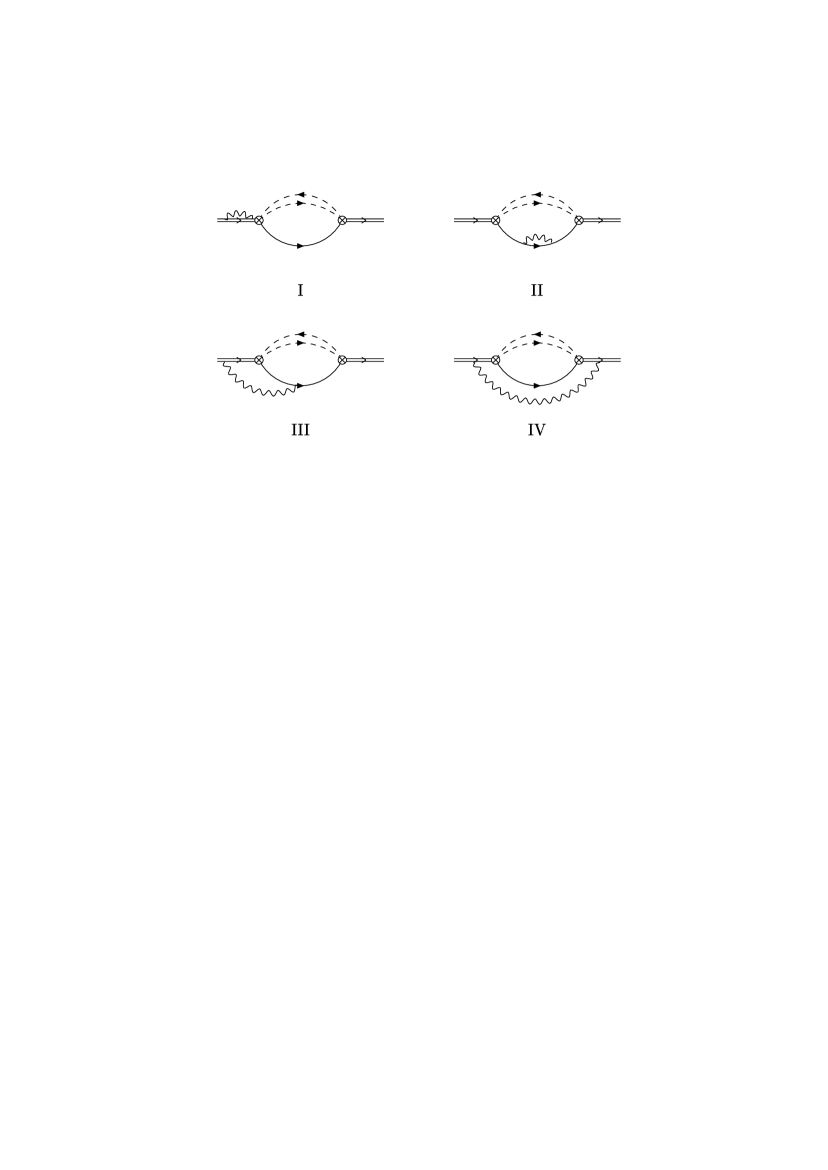
Figure 2: Leading-order radiative corrections to the transition operator, whose imaginary part gives the inclusive semileptonic decay width. Double line: b quark, solid line: c quark, dashed lines: leptons.

For the contribution from the one fermion loop insertion, Smith and Voloshin [19] have derived a useful representation (in the V scheme of [8])

$$d^{V}_{1}(a)=-\int_{0}^{\infty}\frac{d\lambda^{2}}{\lambda^{2}}\left(d_{0}(a,\lambda^{2})-\frac{m_{b}^{2}}{\lambda^{2}+m_{b}^{2}}\right)\,,$$ (2.8)

which has been used in the analysis of Ref. [7]. The calculation of diagrams with multiple fermion loop insertions involves precisely the same function $d_{0}(a,\lambda^{2})$, and can thus be done at little additional calculational expense. In particular, the fixed-order coefficients $d_{n}(a)$ are obtained as [12, 13]

$$d_{n}(a) = \frac{d^{n}}{du^{n}}B[D](a,u)_{|_{u=0}}\,,$$

$$B[D](a,u) = -\frac{\sin(\pi u)}{\pi}\int_{0}^{\infty}\frac{d\lambda^{2}}{\lambda^{2}}\,\left(\frac{\lambda^{2}}{\mu^{2}}e^{C}\right)^{-u}\left[d_{0}(a,\lambda^{2})-1\right]$$ (2.9)

$$= -\frac{\sin(\pi u)}{\pi u}\int_{0}^{\infty}d\lambda^{2}\,\left(\frac{\lambda^{2}}{\mu^{2}}e^{C}\right)^{-u}d^{\prime}_{0}(a,\lambda^{2}),$$

where $d^{\prime}_{0}(a,\lambda^{2})=(d/d\lambda^{2})d_{0}(a,\lambda^{2})$ and $C$ is a scheme-dependent finite renormalization constant. In the $\overline{\rm MS}$ scheme one has $C=-5/3$, in the V scheme $C=0$. It is easy to check that for $n=1$ the above expression reproduces Eq. (2.8).

A closed expression can be derived for the sum of all diagrams with an arbitrary number of fermion bubble insertions [12, 13]:

$$(-\beta_{0}\alpha_{s})M_{\infty}[a,-\beta_{0}\alpha_{s}]=\int_{0}^{\infty}d\lambda^{2}\,\Phi(\lambda^{2})\,d^{\prime}_{0}(a,\lambda^{2})+[d_{0}(a,\lambda_{L}^{2})-1],$$ (2.10)

where $\alpha_{s}=\alpha_{s}(\mu)$,

$$\Phi(\lambda^{2})={}-\frac{1}{\pi}\arctan\left[\frac{-\beta_{0}\alpha_{s}\pi}{1-\beta_{0}\alpha_{s}\ln(\lambda^{2}/\mu^{2}e^{C})}\right]-\,\theta(-\lambda_{L}^{2}-\lambda^{2})\,,$$ (2.11)

and

$$\lambda_{L}^{2}=-\mu^{2}\exp[1/(\beta_{0}\alpha_{s})-C]$$ (2.12)

is the position of the Landau pole in the strong coupling. Note that the term with the $\theta$ function exactly cancels the jump of the $\arctan$ at $\lambda^{2}=-\lambda_{L}^{2}$, so that $\Phi(\lambda^{2})$ is a continuous function of $\lambda^{2}$.

In this paper we cannot give a detailed discussion of the assumptions underlying the derivation of Eqs. (2) and (2.10), and refer the reader to the corresponding sections in [12, 13]. Still, two short comments are appropriate.

First, note that the product $\alpha_{s}(\mu)M_{\infty}[a,-\beta_{0}\alpha_{s}(\mu)]$ is explicitly scale-invariant, provided the running of the coupling is implemented to leading logarithmic accuracy: $\alpha_{s}(\mu_{1})=\alpha_{s}(\mu_{2})/(1-\beta_{0}\alpha_{s}(\mu_{2})\ln(\mu_{1}^{2}/\mu_{2}^{2}))$. This result is also scheme-invariant, and in particular independent of the renormalization constant $C$, provided the couplings are consistently related in the same BLM approximation, that is by keeping only the terms with highest power in $N_{f}$. This is in contrast to the finite order summation coefficients $M_{N}$, which are scheme- and scale-dependent. In the following we assume the $\overline{\rm MS}$ scheme for the coupling $\alpha_{s}$, and the normalization point $\mu=m_{b}$.

Secondly, notice that the second term in (2.10) involves the radiative correction to the decay rate with a finite gluon mass, analytically continued to the Landau pole $\lambda^{2}_{L}<0$. The renormalon divergence of the perturbation theory is reflected [16] by non-analytic terms in the expansion of $d_{0}(a,\lambda^{2})$ at small $\lambda^{2}$ and leads to an imaginary part in this continuation. The size of the imaginary part (divided by $\pi$), $\delta M_{\infty}\equiv 1/(\pi|\beta_{0}|\alpha_{s})\,\mbox{Im}\,d_{0}(a,\lambda^{2}_{L})$, yields an estimate of the ultimate accuracy of perturbation theory, beyond which it has to be complemented by non-perturbative corrections. The real part of (2.10) coincides with the sum of the perturbative series defined by the principal value of the Borel integral [13], and the imaginary part of $d_{0}(a,\lambda^{2}_{L})$ coincides with the imaginary part of the Borel integral.

The calculation of the diagrams in Fig. 2 with a finite gluon mass is straightforward, albeit tedious, and has been undertaken in [7]. Since no formulas were given there, we had to redo this calculation. For $b\to ue\bar{\nu}$ decays, that is for a massless quark in the final state, we have succeeded in obtaining an analytic expression for the decay rate. For $b\to ce\bar{\nu}$ decays, we leave the answer in form of at most two-dimensional integrals and evaluate them numerically. The corresponding formulas are collected in Appendix A.

3 Resummation of BLM-type radiative corrections

Our results are summarized in Table 1.

$$\begin{array}[]{l|rrrrrrrrr}\sqrt{a}&0\phantom{.00}&0.1\phantom{0}&0.2\phantom{0}&0.3\phantom{0}&0.4\phantom{0}&0.5\phantom{0}&0.6\phantom{0}&0.7\phantom{0}&0.99\\ \hline\cr\hline\cr g_{0}&1.81&1.63&1.42&1.25&1.12&1.01&0.92&0.85&0.75\\ \hline\cr d_{0}&1\phantom{.00}&1\phantom{.00}&1\phantom{.00}&1\phantom{.00}&1\phantom{.00}&1\phantom{.00}&1\phantom{.00}&1\phantom{.00}&1\phantom{.00}\\ d_{1}&5.34&5.00&4.55&4.09&3.59&3.10&2.62&2.16&1.18\\ d_{2}&34.4&30.9&27.3&23.9&20.5&17.4&14.3&11.4&5.24\\ \hline\cr M_{0}&1\phantom{.00}&1\phantom{.00}&1\phantom{.00}&1\phantom{.00}&1\phantom{.00}&1\phantom{.00}&1\phantom{.00}&1\phantom{.00}&1\phantom{.00}\\ M_{1}&1.75&1.70&1.64&1.57&1.50&1.43&1.37&1.30&1.17\\ M_{2}&2.42&2.31&2.17&2.04&1.90&1.77&1.65&1.53&1.27\\ M_{\infty}&2.31&2.35&2.24&2.10&1.96&1.82&1.69&1.57&1.38\\ &\ \pm 0.62&\ \pm 0.52&\ \pm 0.44&\ \pm 0.37&\ \pm 0.32&\ \pm 0.26&\ \pm 0.21&\ \pm 0.15&\ \pm 0.03\\ \hline\cr\mu_{1}/m_{b}&0.07&0.08&0.10&0.13&0.17&0.21&0.27&0.34&0.55\\ \mu_{\infty}/m_{b}&0.13&0.13&0.14&0.15&0.17&0.20&0.23&0.27&0.37\\ \hline\cr\hline\cr\end{array}$$

Table 1: Resummation of $\beta_{0}^{n}\alpha_{s}^{n+1}$ corrections for semileptonic B decay widths, see text. The values of $M_{n}$ and $\mu_{n}$ are given for $-\beta_{0}^{(4)}\alpha_{s}(m_{b})=0.14$.

For several representative values of $\sqrt{a}\equiv m_{c}/m_{b}$ we give calculated values of the fixed-order coefficients $d_{n}$, the partial sums $M_{n}$ and the BLM scales $\mu_{n}$. For $n=1$, the $\beta_{0}\alpha_{s}^{2}$ correction, our results coincide with the ones obtained in [7]. We now discuss the numbers in Table 1 in detail.

3.1 Hierarchy of BLM scales

The BLM scale $\mu_{\infty}$ can be larger than the leading-order scale $\mu_{1}$. This may come unexpectedly.

The (leading-order) BLM prescription uses the average of $\ln k^{2}$, the average virtuality of the gluon, as the scale in the coupling. In high orders, this substitution generates a series of radiative corrections with a geometric growth of coefficients $d_{n}\sim(d_{1})^{n}$ to be compared with the factorial growth of the exact coefficients. Resummation to all orders corrects for this discrepancy by adjusting $\mu_{\infty}$ so that the expansion of $\alpha_{s}(\mu_{\infty})$ gives the correct $d_{n}$ for all $n$. Since for this reason for large $n$ the true $d_{n}$ will always outgrow $(d_{1})^{n}$ and since the series is with fixed sign, one might suspect that the usual BLM scale-setting rather underestimates higher-order corrections.

For small c quark masses the effect is opposite, and the very small leading BLM scale $\mu_{1}$ is simply an artefact of truncating the perturbative expansion at low order. The scales $\mu_{1}$ and $\mu_{\infty}$ are given by

$$\mu_{1} = m_{b}\,\exp[-d_{1}/2]=m_{b}\,\exp\left[\frac{1}{2\beta_{0}\alpha_{s}}(M_{1}-1)\right]\,,$$

$$\mu_{\infty} = m_{b}\,\exp\left[\frac{1}{2\beta_{0}\alpha_{s}}\left(1-\frac{1}{M_{\infty}}\right)\right]\,.$$ (3.1)

Although $\delta M\equiv M_{\infty}-M_{1}$ is positive in all cases we consider, the expression in parentheses in the first equation in (3.1) is numerically larger than the similar expression in the second equation, provided $\delta M<(M_{1}-1)^{2}/(2-M_{1})$. This is satisfied for small mass ratios, see Table 1, and results in $\mu_{\infty}>\mu_{1}$ (recall that $\beta_{0}$ is negative with our definition).

Note that the scale $\mu_{\infty}$ is bounded from below: as long as $M_{\infty}$ is positive, $\mu_{\infty}$ is larger than $m_{b}\exp[1/(\beta_{0}\alpha_{s}(m_{b}))]$, the position of the infra-red Landau pole in the running coupling. There is no such restriction for $\mu_{1}$, which can take values below the pole. Again, this is an artefact of the truncation at fixed order.

3.2 Suppression of infra-red contributions for finite c quark mass

With a massive quark in the final state the radiative corrections apparently are reduced: The M-factors $M_{n}$ are smaller, and the BLM scales $\mu_{n}$ are larger. This has been observed in [7] for the BLM scale in leading order, and it continues to all orders, although the difference between $m_{c}/m_{b}=0$ (relevant to $b\to ue\bar{\nu}$ transitions) and $m_{c}/m_{b}=0.3$ is less pronounced after resummation. The ambiguities related to the summation of a divergent series are also reduced and almost vanish in the limit of zero recoil $m_{c}\to m_{b}$. One can understand this by continuing the argument given in the introduction. As explained, these ambiguities arise, because the use of the pole mass parameter implies a static picture, while the energy stored in the field at large distances cannot be converted into hard radiation in the weak decay process. This assumed that the produced quark is fast in the rest frame of the initial b quark. When $m_{c}\to m_{b}$, the c quark is slow. Then, since the long-range part of the field of the b quark is universal, it can be smoothly transferred to the c quark and is simply irrelevant for the description of the decay. Therefore these long-distance contributions cannot be seen in the form of ambiguities in the zero-velocity limit.

To see this more explicitly, we recall that contributions of small momenta to decay rates can be traced by non-analytic terms in the expansion at small values of the gluon mass [16]. For the leading-order radiative correction to the B decay width this expansion takes the form

$$d_{0}(a,\lambda^{2})=1+h_{1}(a)\sqrt{\frac{\lambda^{2}}{m_{b}^{2}}}+h_{2}(a)\frac{\lambda^{2}}{m_{b}^{2}}+\Big{[}h_{31}(a)\ln(\lambda^{2}/m_{b}^{2})+h_{32}(a)\Big{]}\left(\frac{\lambda^{2}}{m_{b}^{2}}\right)^{3/2}+O(\lambda^{4}\ln\lambda^{2})$$ (3.2)

with

$$h_{1}(a) = {}-\frac{\pi}{2f_{1}(a)g_{0}(a)}\Big{[}5-16a^{1/2}-24a-24a^{3/2}+24a^{2}+48a^{5/2}-8a^{3}-8a^{7/2}+3a^{4}$$ (3.3)

$${}-48a^{3/2}\ln a-12a^{2}\ln a\Big{]}\,.$$

Note that the tree-level phase space factor $f_{1}(a)$ and the leading-order radiative correction $g_{0}(a)$ are extracted. The function $h_{1}(a)$ is plotted as a function of the mass ratio $\sqrt{a}=m_{c}/m_{b}$ in Fig. 3.

Figure 3: Coulombic contributions to the B decay rate, Eq. (3.3), expressed in terms of pole masses, as a function of the mass ratio $m_{c}/m_{b}$.

For the realistic value $m_{c}/m_{b}=0.3$ it is reduced by approximately a factor 2 compared to the massless case.

These long-range contributions to the static field are responsible for the major part of the ambiguity in the sum of the perturbative series. Within our approach, this ambiguity is related to the imaginary part of $d_{0}(a,\lambda^{2})$, continued analytically to the position of the Landau pole (2.10), (2.12), and equals

$$(-\beta_{0}\alpha_{s})\delta M_{\infty}=h_{1}(a)\frac{\lambda_{L}}{m_{b}}+O(\lambda_{L}^{3}/m_{b}^{3}).$$ (3.4)

The decrease of the value for $M_{\infty}$ at $\sqrt{a}=0.3$ ($b\to ce\bar{\nu}$ decays) compared to $a=0$ ($b\to ue\bar{\nu}$ decays) roughly equals the decrease of the uncertainty.

In fact, these infra-red contributions are spurious, and can be removed by re-expressing the decay widths in terms of the short-distance (say, $\overline{\rm MS}$) b and c quark masses instead of the pole masses [15, 16]. To trace this cancellation we write e.g. the b quark pole mass $m_{b}$ as related to the running $\overline{\rm MS}$ mass $\overline{m}_{b}$ by the perturbative expansion

$$m_{b}=\overline{m}_{b}(\overline{m}_{b})\Bigg{\{}1+C_{F}\frac{\alpha_{s}(\overline{m}_{b})}{\pi}r_{0}(\lambda^{2})+\ldots\Bigg{\}}\,,$$ (3.5)

where we keep a finite gluon mass $\lambda$ as for the decay width. The expansion of $r_{0}(\lambda^{2})$ at small gluon masses reads [15, 16]:

$$r_{0}(\lambda^{2})=1-\frac{\pi\lambda}{2m_{b}}+\ldots$$ (3.6)

Using Eqs. (3.5), (3.6) and similar expressions for the c quark, we find that, when calculated with a small gluon mass, the tree level decay rate is modified to

$$\Gamma_{0}(a,\lambda)=\Gamma_{0}(a)\left\{1-C_{F}\frac{\alpha_{s}}{\pi}\frac{\pi\lambda}{m_{b}}\left[5/2+(\sqrt{a}-a)\frac{d}{da}\ln f_{1}(a)\right]+\ldots\right\}.$$ (3.7)

It is easy to see that the correction linear in $\lambda$ exactly cancels with a similar term in the radiative correction to the decay width,

$$\Gamma = \Gamma_{0}(a,\lambda)\left[1-C_{F}\frac{\alpha_{s}}{\pi}g_{0}(a)d_{0}(a,\lambda^{2})+\ldots\right]$$ (3.8)

$$= \Gamma_{0}(a)\left[1-C_{F}\frac{\alpha_{s}}{\pi}\frac{\pi\lambda}{m_{b}}\left\{5/2+(\sqrt{a}-a)\frac{d}{da}\ln f_{1}(a)+\frac{1}{\pi}g_{0}(a)h_{1}(a)\right\}+\ldots\right],$$

with the function $h_{1}(a)$ defined as above. The terms in curly brackets add to zero, so that the total decay rate is free from infra-red contributions to this accuracy [15, 16]. It is only the use of a pole mass as an input parameter which introduces infra-red $1/m_{b}$ effects in the tree-level decay rate and in the radiative corrections, which cancel in the product. For a massless quark in the final state several terms in the small-$\lambda$ expansion can easily be obtained analytically, with the result

$$\Gamma=\Gamma_{0}(0)\Bigg{\{}1+C_{F}\frac{\alpha_{s}}{\pi}\Bigg{[}\frac{65}{8}-\frac{\pi^{2}}{2}-\left(\frac{27}{4}+\frac{4\pi^{2}}{3}\right)\frac{\lambda^{2}}{m_{b}^{2}}-\left(\frac{13\pi}{8}+4\pi\ln(\lambda^{2}/m_{b}^{2})\right)\frac{\lambda^{3}}{m_{b}^{3}}+\ldots\Bigg{]}\Bigg{\}}\,.$$ (3.9)

The infra-red contributions now start at order $O(\lambda^{3}/m_{b}^{3}\ln\lambda^{2})$ and are numerically negligible. If so, it is natural to formulate the perturbative calculation in terms of a mass parameter defined at short distances, so that large infra-red contributions do not appear. We address this task now.

$$\begin{array}[]{l|cc|cc|cc}n&r_{n}&M_{n}^{b}&d_{n}(0)&M_{n}^{b\to u}&\overline{d}_{n}(0)&\overline{M}_{n}^{b\to u}\\ \hline\cr\hline\cr 0&1&1&1&1&1&1\\ 1&4.6861511&1.656&5.3381702&1.747&4.3163&1.604\\ 2&17.622650&2.001&34.409913&2.422&8.0992&1.763\\ 3&109.85885&2.303&256.48081&3.126&26.680&1.836\\ 4&873.92393&2.638&2269.4131&3.997&82.262&1.868\\ 5&8839.6860&3.114&23679.005&5.271&421.33&1.890\\ 6&105814.28&3.911&289417.40&7.450&1656.1&1.903\\ 7&1484968.4&5.476&4081180.2&11.75&12135&1.916\\ 8&23740736.&8.978&65496131.&21.42&52862&1.924\\ \hline\cr\infty&-&2.066\pm 0.231&-&2.314\pm 0.615&-&1.925\pm 0.012\\ \hline\cr\hline\cr\end{array}$$

Table 2: Effect of the elimination of the b quark pole mass on the radiative corrections to $b\to ue\bar{\nu}$ decays, see text. The given values of $M_{n}$ correspond to $-\beta_{0}^{(4)}\alpha_{s}(m_{b})=0.14$.

3.3 Elimination of the pole mass: $b\to ue\bar{\nu}$ decays.

The b quark pole mass is related to the $\overline{\rm MS}$ mass by the perturbative series

$$m_{b}=\overline{m}_{b}(\overline{m}_{b})\Bigg{\{}1+C_{F}\frac{\alpha_{s}(\overline{m}_{b})}{\pi}\Big{[}1+\sum_{n=1}^{\infty}\tilde{r}_{n}\alpha_{s}^{n}(\overline{m})\Big{]}\Bigg{\}}\,.$$ (3.10)

As above, we approximate

$$\tilde{r}_{n}=(-\beta_{0})^{n}r_{n}\,,$$ (3.11)

where $r_{n}$ corresponds to contributions of $n$ fermion loops to the leading-order diagram for the fermion self-energy and can be calculated using a representation similar to (2), (2.10) in terms of the leading-order diagram with a finite gluon mass $r_{0}(\lambda^{2})$, see [12, 13] for details. The partial sums for the perturbative series truncated at order $N$ are defined as

$$M_{N}^{b}[-\beta_{0}\alpha_{s}(m_{b})] \equiv 1+\sum_{n=1}^{N}(-\beta_{0})^{n}r_{n}\alpha_{s}^{n}(m_{b})\,,$$

$$M_{\infty}^{b}[-\beta_{0}\alpha_{s}(m_{b})] = M_{N\to\infty}^{b}[-\beta_{0}\alpha_{s}(m_{b})]\,.$$ (3.12)

The coefficients $r_{n}$ were calculated in Ref. [12] and are given together with the partial sums $M_{N}^{b}$ in the second and third columns in Table 2. The perturbative series defining the pole mass is divergent [15, 17], which is reflected by the uncertainty in the factors $M_{\infty}^{b}$. The crucial point is that these uncertainties in defining resummed pole masses are correlated with uncertainties in the resummed radiative correction to the decay rate, and cancel against each other, when the pole mass is defined by its relation to the short-distance mass as in (3.10) or eliminated in favour of the $\overline{\rm MS}$ mass [15, 16].

In what follows we shall consider both possibilities. The first one, which we refer to as calculation in the on-shell scheme (OS), is to define the resummed inclusive decay rate as

$$\Gamma^{OS}(B\to X_{u}e\bar{\nu})=\Gamma_{0}^{OS}\left[1-C_{F}\frac{\alpha_{s}}{\pi}g_{0}(0)M_{\infty}^{b\to u}\right]\,,$$ (3.13)

where it is understood that the b quark pole mass appearing in the tree-level decay rate is substituted by

$$m_{b}=\overline{m}_{b}(\overline{m}_{b})\left[1+C_{F}\frac{\alpha_{s}}{\pi}M_{\infty}^{b}\right]$$ (3.14)

with the factors $M_{\infty}^{b\to u}$ and $M_{\infty}^{b}$ given in Table 2 and the uncertainties deleted.

The second possibility is to use the $\overline{\rm MS}$ scheme from the very beginning. Using (3.10) we can write the decay rate as

$$\Gamma(B\to X_{u}e\bar{\nu})=\overline{\Gamma}_{0}(0)\left\{1+C_{F}\frac{\alpha_{s}(m_{b})}{\pi}\overline{g}_{0}(0)\left[1+\sum_{n=1}^{N}(-\beta_{0})^{n}\overline{d}_{n}(0)\alpha_{s}^{n}(m_{b})\right]\right\}\,,$$ (3.15)

where

$$\overline{g}_{0}(0)=5-g_{0}(0)\,,\qquad\overline{d}_{n}(0)=-\frac{g_{0}(0)d_{n}(0)-5r_{n}}{\overline{g}_{0}(0)}\,,$$ (3.16)

and the tree-level decay rate $\overline{\Gamma}_{0}$ is expressed in terms of $\overline{m}_{b}(\overline{m}_{b})$. Note that the leading-order radiative correction changes sign and becomes somewhat larger.

The coefficients $\overline{d}_{n}$ and partial sums $\overline{M}_{N}^{b\to u}$ defined in an obvious way in analogy to (2) are given in Table 2 in comparison to $d_{n}$ and $M_{N}^{b\to u}$, respectively. It is seen that the coefficients are drastically reduced, and the series has become well convergent. The remaining infra-red effects, relevant to the divergence of the perturbative series, are suppressed by three powers of the b quark mass [16] and have become tiny. Most importantly, this improvement is effective already at $n=2$. We conclude that perturbative coefficients in the $\overline{\rm MS}$ scheme are likely to be much smaller than in the OS scheme without restriction to vacuum polarization corrections, too.

In the framework of a purely perturbative calculation the use of the OS scheme can only be justified up to the order where perturbative series diverge. In all-order resummations such as the one considered in this paper, one must make sure that the prescription defining the pole mass in terms of a short-distance mass or any physical quantity is consistent with the prescription to sum the perturbative series of radiative corrections to the decay width. Even in this case, the OS scheme is somewhat unnatural since it involves large cancellations between radiative corrections to decay rates and to the pole masses already in low orders.

The resummed decay rate in the $\overline{\rm MS}$ scheme is readily obtained by inserting (3.14) into (3.13) and expanding up to $O(\alpha_{s})$:

$$\overline{\Gamma}=\overline{\Gamma}_{0}\left\{1+C_{F}\frac{\alpha_{s}}{\pi}\Big{[}5M_{\infty}^{b}-g_{0}(0)M_{\infty}^{b\to u}\Big{]}\right\}\,.$$ (3.17)

The difference between (3.13) and (3.17) is an effect of order $(C_{F}\alpha_{s}/\pi)^{2}$, which is beyond our accuracy. It is a pure scheme dependence, resulting from our incomplete perturbative calculation. Numerically, the difference amounts to about 6%, which is significantly smaller than the $\pm 15\%$ uncertainty for the radiative corrections noted in the introduction.

3.4 Elimination of the pole mass: $b\to ce\bar{\nu}$ decays.

Expressing the $b\to ce\bar{\nu}$ decay rate in terms of the running masses is slightly more cumbersome. As above, we start with the resummed decay rate in the OS scheme

$$\Gamma^{OS}(B\to X_{c}e\bar{\nu})=\Gamma_{0}^{OS}\left[1-C_{F}\frac{\alpha_{s}}{\pi}g_{0}(a)M_{\infty}^{b\to c}\right]\,,$$ (3.18)

where now both the c and b quark masses have to be expressed in terms of the running masses. Here we want to be somewhat more general, and introduce running masses at arbitrary scale $\mu$ as

$$m_{c,b}=\overline{m}_{c,b}(\mu)\Big{[}1+C_{F}\frac{\alpha_{s}(\mu)}{\pi}\overline{M}_{\infty}^{c,b}(\mu)\Big{]}\,.$$ (3.19)

The factors $\overline{M}_{\infty}^{c}(\mu)$ and $\overline{M}_{\infty}^{b}(\mu)$ can most easily be calculated by observing that the pole mass on the left-hand side of (3.19) is scheme-invariant, and using the renormalization-group expression for the running mass

$$\bar{m}(\mu)=\bar{m}(\bar{m})\,\exp\left(\,\,-\frac{1}{\beta_{0}}\int_{\alpha_{s}(m)}^{\alpha_{s}(\mu)}\frac{d\alpha}{\alpha^{2}}\,\gamma_{m}(\alpha)\right)\,,$$ (3.20)

where to our accuracy we have to expand the exponential to first order, but keep the mass anomalous dimension to all orders in $\beta_{0}^{n}\alpha_{s}^{n+1}$, which is known from [22, 13] (see Eq. (4.19) in [13]):

$$\gamma_{m}(\alpha_{s})=\frac{\alpha_{s}}{\pi}\Bigg{[}1-\frac{5}{6}(\beta_{0}\alpha_{s})-\frac{35}{36}(\beta_{0}\alpha_{s})^{2}+\ldots\Bigg{]}.$$ (3.21)

Thus, we obtain, e.g. for the c quark

$$C_{F}\frac{\alpha_{s}(\mu)}{\pi}\overline{M}_{\infty}^{c}(\mu)=C_{F}\frac{\alpha_{s}(m_{c})}{\pi}M_{\infty}^{c}+\frac{1}{\beta_{0}}\int_{\alpha_{s}(m_{c})}^{\alpha_{s}(\mu)}\frac{d\alpha}{\alpha^{2}}\,\gamma_{m}(\alpha),$$ (3.22)

where $M_{\infty}^{c}$ is a factor relating the c quark pole mass to the running mass $\overline{m}_{c}(\overline{m}_{c})$, defined as in (3.14).

Collecting everything, we find

$$\overline{\Gamma}(B\to X_{c}e\bar{\nu}) = \overline{\Gamma}_{0}(\bar{a},\mu)\left\{1+C_{F}\frac{\alpha_{s}(\mu)}{\pi}\Big{[}5\overline{M}_{\infty}^{b}(\mu)-g_{0}(\bar{a})M_{\infty}^{b\to c}\right.$$ (3.23)

$$\left.{}\hskip 28.45274pt+2\Big{(}\overline{M}_{\infty}^{c}(\mu)-\overline{M}_{\infty}^{b}(\mu)\Big{)}\bar{a}\frac{d}{d\bar{a}}\ln f_{1}(\bar{a})\Big{]}\right\},$$

where $\bar{a}=(\bar{m}_{c}(\mu)/\bar{m}_{b}(\mu))^{2}$. It is worth while to note that the factor that appears in front of the logarithmic derivative of the phase space function $f_{1}$ is scale-independent:

$$\alpha_{s}(\mu)\Big{(}\overline{M}_{\infty}^{c}(\mu)-\overline{M}_{\infty}^{b}(\mu)\Big{)}=\alpha_{s}(m_{c})M_{\infty}^{c}-\alpha_{s}(m_{b})M_{\infty}^{b}+\frac{\pi}{\beta_{0}C_{F}}\int_{\alpha_{s}(m_{c})}^{\alpha_{s}(m_{b})}\frac{d\alpha}{\alpha^{2}}\,\gamma_{m}(\alpha)\,.$$ (3.24)

The expression in (3.23) is to be compared with the leading-order decay rate [18]:

$$\overline{\Gamma}^{LO}(B\to X_{c}e\bar{\nu}) = \overline{\Gamma}_{0}(\bar{a},\mu)\left\{1+C_{F}\frac{\alpha_{s}(\mu)}{\pi}\bar{g}_{0}(\bar{a},\mu)\right\}\,,$$

$$\bar{g}_{0}(\bar{a},\mu) = 5-g_{0}(\bar{a})-\frac{15}{4}\ln\frac{m_{b}^{2}}{\mu^{2}}-\frac{3}{2}\bar{a}\ln\bar{a}\frac{d}{d\bar{a}}\ln f_{1}(\bar{a})\,.$$ (3.25)

To quantify the effect of resummation, we introduce the corresponding M-factor by rewriting the resummed result in (3.23) as

$$\overline{\Gamma}(B\to X_{c}e\bar{\nu}) = \overline{\Gamma}_{0}(\bar{a},\mu)\left\{1+C_{F}\frac{\alpha_{s}(\mu)}{\pi}\bar{g}_{0}(\bar{a},\mu)\overline{M}^{b\to c}_{\infty}(\mu)\right\}\,.$$ (3.26)

We give the corresponding values in Table 7 for $\mu=\overline{m}_{b}$. Tracing the scale dependence of $\overline{M}_{\infty}(\mu)$ is misleading in this case because $\bar{g}_{0}(\bar{a},\mu)$ is strongly scale-dependent.

3.5 The SV limit and exclusive B decays

The inclusive decay rate in the Shifman-Voloshin (SV) limit $m_{b},\,m_{c}\gg m_{b}-m_{c}\gg\Lambda_{\rm\scriptsize QCD}$ [23] is dominated by two exclusive decay channels, $B\to De\bar{\nu}$ and $B\to D^{*}e\bar{\nu}$. Since the final state meson is produced almost at rest (in leading order in the heavy quark expansion), the techniques of the Heavy Quark Effective Theory are applicable, yielding the decay rate

$$\Gamma(B\to De\bar{\nu},D^{*}e\bar{\nu})=\frac{G_{F}^{2}|V_{cb}|^{2}(m_{b}-m_{c})^{5}}{60\pi^{3}}\left(\eta_{V}^{2}+3\eta_{A}^{2}\right),$$ (3.27)

where $\eta_{V}$ and $\eta_{A}$ are the short-distance matching coefficients of the QCD heavy-heavy currents to the corresponding currents in the effective theory (at zero recoil):

$$\bar{c}\gamma_{\mu}b=\eta_{V}\bar{h}_{c}\gamma_{\mu}h_{b}+O(1/m^{2}),\quad\bar{c}\gamma_{\mu}\gamma_{5}b=\eta_{A}\bar{h}_{c}\gamma_{\mu}\gamma_{5}h_{b}+O(1/m^{2}).$$ (3.28)

They are given by a perturbative series, in which, as above, we only keep the BLM-type $\beta_{0}^{n}\alpha_{s}^{n+1}$ terms ($z=m_{c}/m_{b}$):

$$\eta_{V,A}=1+C_{F}\,\frac{\alpha_{s}(m_{b})}{\pi}\,r_{0}^{V,A}(z)\left[1+\sum_{n=1}^{\infty}(-\beta_{0})^{n}d_{n}^{V,A}\alpha_{s}^{n}(m_{b})\right]$$ (3.29)

with [24, 23]

$$r_{0}^{V}(z)=-\frac{3}{2}-\frac{3}{4}\,\frac{1+z}{1-z}\,\ln\,z,\quad r_{0}^{A}(z)=-2-\frac{3}{4}\,\frac{1+z}{1-z}\,\ln\,z\,.$$ (3.30)

The resummation of $\beta_{0}^{n}\alpha_{s}^{n+1}$ terms for the $\eta$’s was discussed in some detail in [9, 11] and can equally easily be implemented within our dispersion technique. For completeness, we collect the necessary formulas in Appendix B. The results are summarized in Table 3, where we give the leading-order coefficients $d_{1}^{V,A}$ and the resummed enhancement factors

$$M^{V,A}_{\infty}[a,-\beta_{0}\alpha_{s}(m_{b})]\equiv 1+\sum_{n=1}^{\infty}(-\beta_{0})^{n}d_{n}\alpha_{s}^{n}(m_{b})\,.$$ (3.31)

$$\begin{array}[]{c|cc|cc}m_{c}/m_{b}&d_{1}^{V}&d_{1}^{A}&M_{\infty}^{V}&M_{\infty}^{A}\\ \hline\cr\hline\cr 0.1&2.47&1.63&2.07\pm 0.05&2.69\pm 1.09\\ 0.2&1.78&3.32&1.50\pm 0.07&2.37\pm 0.42\\ 0.3&1.36&2.56&1.30\pm 0.06&1.96\pm 0.16\\ 0.4&1.08&2.17&1.20\pm 0.05&1.76\pm 0.09\\ 0.5&0.86&1.90&1.14\pm 0.04&1.64\pm 0.06\\ 0.6&0.68&1.70&1.09\pm 0.03&1.56\pm 0.05\\ 0.7&0.52&1.53&1.06\pm 0.03&1.50\pm 0.04\\ 0.8&0.39&1.39&1.04\pm 0.03&1.45\pm 0.03\\ 0.9&0.27&1.27&1.02\pm 0.02&1.41\pm 0.03\\ 1&0.17&1.17&1.00&1.37\pm 0.03\\ \hline\cr\hline\cr\end{array}$$

Table 3: The lowest-order coefficients $d_{1}^{V,A}$ and the resummed series $M_{\infty}^{V,A}$ for $\eta_{V,A}$ in the $\overline{\rm MS}$ scheme as functions of the ratio of pole masses $m_{c}/m_{b}$. Note that the expressions diverge for $m_{c}\to 0$. For $m_{c}=m_{b}$, $\eta_{V}\equiv 1$ due to charge conservation. Input parameter: $-\beta_{0}\alpha_{s}(m_{b})=0.14$.

To make an explicit comparison to inclusive decays possible, we have presented the results in the form of an expansion in $\alpha_{s}(m_{b})$ rather than in $\alpha_{s}(\sqrt{m_{b}m_{c}})$ which is more natural in exclusive decays. Because of this, our coefficients are related to the ones given in Ref. [9] by $d_{1}^{V,A}(\mu=\sqrt{m_{b}m_{c}})=d_{1}^{V,A}(\mu=m_{b})+\ln m_{c}/m_{b}$. Since the product of $\alpha_{s}$ and $M_{\infty}$ is scale-independent, when a one-loop running coupling is used, we have

$$M^{V,A}_{\infty}[z,-\beta_{0}\alpha_{s}(\sqrt{m_{b}m_{c}})]\,=\,\frac{\alpha_{s}(m_{b})}{\alpha_{s}(\sqrt{m_{b}m_{c}})}\,M^{V,A}_{\infty}[z,-\beta_{0}\alpha_{s}(m_{b})]\,.$$ (3.32)

Thus, for example, with $\alpha_{s}(m_{b})/\alpha_{s}(\sqrt{m_{b}m_{c}})=0.82$ and $M^{A}_{\infty}[0.3,-\beta_{0}\alpha_{s}(m_{b})]=1.96$ from Table 3, we get $M^{A}_{\infty}[0.3,-\beta_{0}\alpha_{s}(\sqrt{m_{b}m_{c}})]=1.59$. Note that this number is rather large and indicates that the higher-order corrections are important in the axial channel.

Where a comparison is possible, our results agree with the values obtained in [11]. We obtain

$$\eta_{A}=0.943\pm 0.005\pm 0.010\pm 0.001,$$ (3.33)

where the first error gives the estimated renormalon uncertainty, the second one the uncertainty coming from $\alpha_{s}(m_{Z})$, and the third one the uncertainty in the input quark masses.

In the limit $m_{c}\to m_{b}$ the inclusive decay rate thus equals (in perturbation theory)

$$\Gamma(B\to X_{c}e\bar{\nu})=\frac{G_{F}^{2}|V_{cb}|^{2}(m_{b}-m_{c})^{5}}{15\pi^{3}}\,\left\{1-C_{F}\,\frac{\alpha_{s}(m_{b})}{\pi}\,\frac{3}{4}\,M_{\infty}^{A}(a=1)\right\},$$ (3.34)

which implies the relation

$$M_{\infty}^{b\to c}(a=1)\equiv M_{\infty}^{A}(a=1)$$ (3.35)

and provides a non-trivial check of our calculation. Comparing the corresponding entries in Table 1 and Table 3 we indeed find agreement.

4 Determination of $|V_{cb}|$

4.1 Theoretical input parameters

The main parameters we need in order to determine $|V_{cb}|$ are the b and the c quark masses. At present there seems to be no general consensus on their values, and the existing estimates are often controversial. The masses extracted from the spectroscopy of $\bar{b}b$ and $\bar{c}c$ mesons are usually given with very small errors, see e.g. Ref. [25]. However, the actual uncertainty is in this case hidden in their relation to the running masses at a certain hard scale, which we need in this paper. Thus, we prefer to rely on a less accurate (as far as numbers are concerned) direct determination of the $\overline{\rm MS}$ b quark mass from QCD sum rules for lowest moments of $e^{+}e^{-}$ annihilation to heavy quarks [26, 27]. Due to the smaller scales involved, such estimates are less reliable for the c quark mass, so that we prefer to fix $m_{c}$ by a different method, see below. In this paper we use the following value for the $\overline{\rm MS}$ b quark mass [28, 29]:

$$\overline{m}_{b}(\overline{m}_{b}) = (4.23\pm 0.05)\,\mbox{\rm GeV.}$$ (4.1)

We point out that $\overline{m}_{b}$ was chosen as renormalization point mainly in order to conform to the standard choice in the literature, in the same way as $\alpha_{s}$ is usually normalized by its value at the Z boson mass. Actually in our approach the question of the “natural” scale does not appear, at least to the extent that the approximation of summing higher order corrections due to vacuum polarization is good: all results are explicitly scale-invariant for a one-loop running coupling. In finite order perturbative calculations it may be more appropriate to choose a lower renormalization scale in order to minimize the size of uncalculated higher order terms. From (4.1) we get the pole mass

$$m_{b} = (5.05\pm 0.06)\,\mbox{\rm GeV,}$$ (4.2)

where all radiative corrections of type $\beta_{0}^{n}\alpha_{s}^{n+1}$ are resummed. Very similar values for the b quark pole mass were proposed in Refs. [30, 20] and are also indicated by lattice calculations [31].

In order to fix the c quark mass, we make use of the fact that the difference between the pole masses of two heavy quarks is free from many ambiguities intrinsic in the mass parameters themselves and can be determined to a good accuracy from the expansion

$$m_{b}-m_{c}=m_{B}-m_{D}+\frac{1}{2}\left(\frac{1}{m_{b}}-\frac{1}{m_{c}}\right)\Big{[}\lambda_{1}+3\lambda_{2}\Big{]}+O(\alpha_{s}/m,1/m^{2}),$$ (4.3)

where $m_{B}$ and $m_{D}$ are the B and D meson masses, respectively; $\lambda_{2}$ is given by

$$\lambda_{2}\simeq\frac{1}{4}(m^{2}_{B^{*}}-m^{2}_{B})\simeq 0.12\,\mbox{\rm GeV}^{2},$$ (4.4)

and $-\lambda_{1}/(2m_{b})$ is the kinetic energy of a heavy quark inside a B meson. For $\lambda_{1}$ an estimate is available from QCD sum rules [32], $\lambda_{1}=-(0.6\pm 0.1)\,$GeV², which is however strongly correlated with the value of $\bar{\Lambda}=m_{B}-m_{b}$ and thus with the value of the b quark pole mass. The estimate quoted in [32] is the average of $\lambda_{1}=-0.5\,$GeV² and $-0.7\,$GeV² obtained for $\bar{\Lambda}=400\,$MeV and $500\,$MeV, respectively. The resummation of $\beta_{0}^{n}\alpha_{s}^{n+1}$ radiative corrections leads to a significant increase of the value of the b quark pole mass, and thus to a much lower value of $\bar{\Lambda}$ of order (200–300) MeV. Thus in principle the value for $\lambda_{1}$ to be used in our analysis should be obtained from a QCD sum rule using a small value of $\bar{\Lambda}$ and including the resummation of running coupling effects, which is not available. We have calculated the BLM-type $\alpha_{s}^{2}$ correction to the simpler sum rule for the leptonic decay constant $f_{B}$ in the static limit [33], which also enters the sum rule for $\lambda_{1}$ as normalization factor, and found that this correction is very small (in other words: the BLM scale coincides with the “naive” hard scale). This may be accidental, however, and rather indicate that other corrections are important. We have also checked that the sum rule for $\lambda_{1}$ derived in [32] becomes much less sensitive to the value of $\bar{\Lambda}$ if it is small, and even with arbitrary $\bar{\Lambda}$ it is not possible to push $-\lambda_{1}$ below (0.25–0.30) GeV². Lacking a BLM-improved sum rule for $\lambda_{1}$, we consider $-(0.5\pm 0.2)\,$GeV² as a fair estimate. With this value, one obtains from (4.3)

$$m_{b}-m_{c}=(3.43\pm 0.04)\,\mbox{\rm GeV}\,,$$ (4.5)

assuming that $\alpha_{s}/m$ and $1/m^{2}$ corrections in (4.3) are negligible. Combining this result with the b quark pole mass in (4.2) we get the c quark pole mass

$$m_{c}=(1.62\pm 0.07)\,\mbox{\rm GeV}$$ (4.6)

and the running mass

$$\overline{m}_{c}(\overline{m}_{c})=(1.29\pm 0.06)\,\mbox{\rm GeV}\,.$$ (4.7)

This value is consistent with determinations from QCD sum rules [26, 27].

For completeness, we also give the corresponding values of the “one-loop pole masses” defined as

$$m^{(1)}_{b,c} = \overline{m}_{b,c}(\overline{m}_{b,c})\Bigg{\{}1+C_{F}\frac{\alpha_{s}(\overline{m}_{b,c})}{\pi}\Bigg{\}}:$$ (4.8)

$$m^{(1)}_{c} = (1.50\pm 0.06)\,\mbox{\rm GeV}\,,$$

$$m^{(1)}_{b} = (4.63\pm 0.05)\,\mbox{\rm GeV}\,.$$ (4.9)

Our values are in agreement with those quoted in Ref. [30].

4.2 Extraction of $|V_{cb}|$

Our discussion was so far restricted to the perturbative corrections to the b quark decay rate. In order to extract $|V_{cb}|$ from the experimental data, we now have to specify the non-perturbative corrections, which are suppressed by two powers of the heavy quark masses. Summarizing the results of Refs. [6, 32, 34] we write

$$\Gamma(B\to X_{c}e\bar{\nu})=\Gamma(B\to X_{c}e\bar{\nu})_{pert}\left(1+\frac{\delta^{NP}}{m_{b}^{2}}\right)$$ (4.10)

with $\delta^{NP}=-(1.05\pm 0.10)\,{\rm GeV}^{2}$, where the error comes from the uncertainty in $\lambda_{1}$, cf. Sec. 4.1.

As for the exclusive decays, the experimentally interesting quantity is the differential decay rate at zero recoil of the final state meson, which depends on the form factor

$${\cal F}(1)=\eta_{A}(1+\delta_{1/m^{2}}).$$ (4.11)

The short-distance correction $\eta_{A}$ was already discussed in Sec. 3.5; numerical values are given there and in Table 7 below. The non-perturbative correction $\delta_{1/m^{2}}$ was estimated in Refs. [2] as $-(5.5\pm 2.5)\%$ using $\lambda_{1}=-0.4$ GeV².

As experimental input we use the world average $B^{0}$ lifetime $\tau_{B^{0}}=1.5\,$ps [36], the most recent measurement of the $B^{0}$ semileptonic branching ratio $B_{SL}=(10.9\pm 1.3)\%$ [37], and $|V_{cb}{\cal F}(1)|=0.0354\pm 0.0027$ [38], where we have rescaled the latter value to be compatible with $\tau_{B^{0}}=1.5\,$ps.

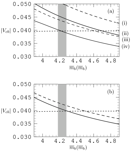
Figure 4: The value of $|V_{cb}|$ extracted from the inclusive B meson semileptonic decay rate to one-loop accuracy (a) [the curves (i) to (iv) are explained in the text] and after resumming $\beta_{0}^{n}\alpha_{s}^{n+1}$ radiative corrections (b) as a function of the $\overline{\rm MS}$ b quark mass for fixed $\lambda_{1}=-0.5\,$GeV². The solid and long-dashed curves show the predictions obtained by using the $\overline{\rm MS}$ and OS scheme, respectively. The central value coming from exclusive decays is shown by short dashes and the shaded area gives the interval of b quark mass values suggested by QCD sum rules, Eq. (4.1). Experimental input: $\tau_{B^{0}}=1.5\,$ps, $B_{SL}=10.9\%$, $\alpha_{s}(m_{Z})=0.117$.

$$\begin{array}[]{cl|lllll}&\overline{m}_{b}(\overline{m}_{b})&4.0&4.1&4.2&4.3&4.4\\ &\lx@intercol\hfil m_{b}\lx@intercol\vrule\lx@intercol&4.80^{+(9)}_{-(9)}&4.91^{+(9)}_{-(9)}&5.02^{+(9)}_{-(9)}&5.13^{+(9)}_{-(9)}&5.24^{+(9)}_{-(9)}\\ \overline{m}_{c}(\overline{m}_{c})&m_{c}\\ \hline\cr\hline\cr&\\[-14.0pt] 1.18&1.47^{-(6)}_{+(1)}&0.045^{-(3)}_{+(3)}&0.042^{-(3)}_{+(2)}&0.039^{-(2)}_{+(2)}&0.037^{-(2)}_{+(2)}&0.034^{-(2)}_{+(2)}\\[4.0pt] 1.22&1.52^{-(5)}_{+(0)}&0.046^{-(3)}_{+(3)}&0.043^{-(3)}_{+(2)}&0.040^{-(2)}_{+(2)}&0.037^{-(2)}_{+(2)}&0.035^{-(2)}_{+(2)}\\[4.0pt] 1.26&1.58^{-(4)}_{+(0)}&0.047^{-(3)}_{+(3)}&0.044^{-(3)}_{+(2)}&0.041^{-(2)}_{+(2)}&0.038^{-(2)}_{+(2)}&0.035^{-(2)}_{+(2)}\\[4.0pt] 1.30&1.63^{-(4)}_{+(0)}&0.048^{-(3)}_{+(3)}&0.045^{-(3)}_{+(2)}&0.041^{-(3)}_{+(2)}&0.039^{-(2)}_{+(2)}&0.036^{-(2)}_{+(2)}\\[4.0pt] 1.34&1.68^{-(3)}_{-(1)}&0.049^{-(3)}_{+(3)}&0.046^{-(3)}_{+(3)}&0.042^{-(3)}_{+(2)}&0.039^{-(2)}_{+(2)}&0.037^{-(2)}_{+(2)}\\[4.0pt] \hline\cr\hline\cr\end{array}$$

Table 4: $|V_{cb}|$ calculated in the $\overline{\rm MS}$ scheme for a wide range of quark masses. The central value is obtained for $\alpha_{s}(m_{Z})=0.117$, the upper (lower) number in brackets gives the shift of the last digit if $\alpha_{s}$ is put to $0.123$ ($0.111$). The masses are given in GeV. Experimental input: $B_{SL}=10.9$%, $\tau_{B^{0}}=1.5\,$ps.

$$\begin{array}[]{cc|lllll}&\lx@intercol\hfil\overline{m}_{b}(\overline{m}_{b})\lx@intercol\vrule\lx@intercol&4.0&4.1&4.2&4.3&4.4\\ &\lx@intercol\hfil m_{b}\lx@intercol\vrule\lx@intercol&4.80^{+(9)}_{-(9)}&4.91^{+(9)}_{-(9)}&5.02^{+(9)}_{-(9)}&5.13^{+(9)}_{-(9)}&5.24^{+(9)}_{-(9)}\\ \lambda_{1}\,[{\rm GeV}^{2}]&\lx@intercol m_{b}-m_{c}\hfil\lx@intercol\vrule\lx@intercol\\ \hline\cr\hline\cr&\\[-14.0pt] -0.3&3.39&0.0441^{-(7)}_{+(7)}&0.0426^{-(7)}_{+(7)}&0.0414^{-(7)}_{+(7)}&0.0402^{-(7)}_{+(7)}&0.0392^{-(6)}_{+(6)}\\[4.0pt] -0.4&3.41&0.0438^{-(7)}_{+(7)}&0.0423^{-(7)}_{+(7)}&0.0411^{-(6)}_{+(7)}&0.0399^{-(6)}_{+(6)}&0.0389^{-(6)}_{+(6)}\\[4.0pt] -0.5&3.43&0.0434^{-(6)}_{+(7)}&0.0420^{-(6)}_{+(6)}&0.0408^{-(6)}_{+(6)}&0.0397^{-(6)}_{+(6)}&0.0387^{-(6)}_{+(6)}\\[4.0pt] -0.6&3.46&0.0431^{-(6)}_{+(6)}&0.0417^{-(6)}_{+(6)}&0.0405^{-(6)}_{+(6)}&0.0394^{-(6)}_{+(6)}&0.0384^{-(6)}_{+(6)}\\[4.0pt] -0.7&3.48&0.0427^{-(6)}_{+(6)}&0.0414^{-(6)}_{+(6)}&0.0402^{-(6)}_{+(6)}&0.0391^{-(6)}_{+(6)}&0.0382^{-(5)}_{+(5)}\\[4.0pt] \hline\cr\hline\cr\end{array}$$

Table 5: $|V_{cb}|$ calculated in the $\overline{\rm MS}$ scheme in dependence on the b quark mass and $\lambda_{1}$. Notations and experimental input as in the previous table.

Our results are summarized in Fig. 4 and in Tables 5 and 5, where we give $|V_{cb}|$ as function of the running b quark mass. The determination with one-loop radiative corrections is plotted in Fig. 4(a) and using resummation in Fig. 4(b). The solid line represents the result from the $\overline{\rm MS}$, the long dashes from the OS calculation. The short dashes give $|V_{cb}|$ from exclusive decays. The shaded areas illustrate the range of b quark mass values from Eq. (4.1). The curves in Fig. 4(b) are obtained for $\lambda_{1}=-0.5\,$GeV², which corresponds roughly to a fixed difference of the pole masses of $m_{b}-m_{c}=3.43\,$GeV.

The two sets of curves in Fig. 4(a) are obtained with two different ways to specify the c quark mass. The first way is to use exactly the same short-distance c quark mass as in Fig. 4(b): the curves labelled (i) and (ii) are obtained using the constraint (4.3) with resummed pole masses, i.e. fixing $m_{b}-m_{c}=3.43\,$GeV, and calculating $m_{c}^{(1)}$ and $\overline{m}_{c}(\overline{m}_{c})$, respectively, for a given value of $\overline{m}_{b}(\overline{m}_{b})$. Thus, since all short-distance input parameters are chosen in precisely the same way as in Fig. 4(b), the difference between the predictions for $|V_{cb}|$ is entirely the effect of resummation.

Although this choice is presumably the most clear way to show the effect of resummation of running coupling effects, it also may be slightly misleading. Indeed, the large difference in values of $|V_{cb}|$ between the one-loop and resummed formulas is mainly due to the fact that the one-loop pole masses defined in this way do not satisfy Eq. (4.3): $m_{b}^{(1)}-m_{c}^{(1)}=3.13\,$GeV. Thus we also try another choice, calculating the c quark mass by enforcing the constraint (4.3) expressed in terms of one-loop pole masses, so that $m_{b}^{(1)}-m_{c}^{(1)}=3.43\,$GeV. The results are shown in the form of curves (iii) and (iv). This choice is less instructive as far as the comparison between one-loop and resummed results is concerned, but is probably more attractive phenomenologically. On the other hand, we note that with this choice the value of the short-distance c quark mass becomes very low, $\overline{m}_{c}(\overline{m}_{c})=0.98\,$GeV [$m_{c}^{(1)}=1.18\,$GeV] for $\overline{m}_{b}(\overline{m}_{b})=4.23\,$GeV, which is hardly consistent with the QCD sum rules for the charmonium system. The large difference in the resulting values for $|V_{cb}|$ shows the dilemma all strict one-loop calculations are inevitably confronted with: it is impossible to relate the three independently determined input parameters $\overline{m}_{b}(\overline{m}_{b})$, $\overline{m}_{c}(\overline{m}_{c})$ and $\lambda_{1}$ to each other within the errors by one-loop equations, although all of them provide valid phenomenological input. It is only after inclusion of higher order perturbative corrections in Eq. (4.3) in form of the resummed pole masses that the three values appear to be consistent with each other, and it may be considered as a serious argument in favour of BLM-improved perturbation theory in semileptonic inclusive decays that the central value (but not the error bars, see below) of $|V_{cb}|$ is independent of the choice of a particular subset.

The effect of resummation is clearly visible in Fig. 4(b): first, we find a considerably reduced scheme dependence, i.e. the difference between the solid and the long-dashed curves is much smaller in Fig. 4(b) than in Fig. 4(a). Secondly, we observe good agreement between $|V_{cb}|$ from exclusive and inclusive decays obtained with resummation, which otherwise is only achieved for either an unreasonably large b quark mass or a very small c quark mass.

It has been proposed in Ref. [35] that in inclusive decays the dependence on the quark masses is significantly reduced, if the charm and bottom masses are not varied independently, but related to each other by Eq. (4.3). To study this question, we give tables of numerical values for $|V_{cb}|$, choosing as independent input parameters either the running b and c quark masses (Table 5), or the running b quark mass and $\lambda_{1}$, which specifies the difference between the pole masses (Table 5). It is clearly seen that, although the central values for $|V_{cb}|$ are nearly the same, the latter choice is preferable, since the inclusive decay rate is very sensitive to the mass difference $m_{b}-m_{c}$, and already a very modest accuracy in $\lambda_{1}$ in fact constrains $m_{b}-m_{c}$ more precisely than any direct determination. We conclude that $\lambda_{1}$ (or equivalently $m_{b}-m_{c}$) is a better theoretical input parameter than the c quark mass itself, in agreement with the discussion in Ref. [35]. In addition we find that the dependence on $\alpha_{s}(m_{Z})$ is strongly reduced, too. We emphasize, however, that our choice of input parameters only serves to reduce the sensitivity of $|V_{cb}|$ on uncertainties in the input parameters and that the central value is independent of that choice.

It might also be useful to compare the results obtained from the resummed formulas with those obtained in the usual BLM approximation, where of the whole series of corrections generated by the running of the coupling only the $\alpha_{s}^{2}\beta_{0}$ term is taken into account. Again, the major subtlety comes from the necessity to specify the c quark mass. It turns out that the perturbative series that relates the c quark pole mass to the $\overline{\rm MS}$ mass starts to diverge already in second order [12]. Because of the divergence, it is not justified to cut the series at that order, although in this case the BLM correction gives an excellent approximation to the exact two-loop result. For example, starting from $\overline{m}_{c}(\overline{m}_{c})=1.26\,$GeV one gets for the BLM pole mass $m_{c}^{BLM}=1.75$ GeV, which is significantly larger than the resummed result $m_{c}=1.58$ GeV. In other words, the BLM approximation underestimates the scale of the coupling and thus overestimates the radiative correction. A comparison between the BLM and the resummed results is however possible if one starts from the $\overline{\rm MS}$ b quark mass, calculates the b quark pole mass in the BLM approximation, and then fixes the c quark pole mass from the heavy-quark expansion (4.3). Taking for definiteness $\overline{m}_{b}(\overline{m}_{b})=4.23\,$GeV and $\lambda_{1}=-0.5\,$GeV², we find in this way in the BLM approximation $|V_{cb}|=0.0381$ ($|V_{cb}|=0.0424$) in the $\overline{\rm MS}$ (OS) scheme, respectively, compared with $|V_{cb}|=0.0404$ ($|V_{cb}|=0.0424$) with resummed formulas. The perfect agreement between the BLM and resummed formulas in the OS scheme is probably accidental. In the $\overline{\rm MS}$ (OS) scheme the BLM result is very close to the one-loop calculation, see Fig. 4. In both cases, the numerical effect of higher order corrections is small and of the order of 5%. We wish to emphasize once more, however, that this comparison is only possible if the c quark mass is obtained in a very particular way and it is only after resummation that we are able to get a selfconsistent description in terms of short-distance parameters.

From the combined evidence of Fig. 4 and Tables 5 and 5 we extract the following results:

$$|V_{cb}|^{\overline{\rm\scriptsize MS}} = (0.0404\pm 0.0006\pm 0.0006\pm 0.0006)\,\left(\frac{B_{SL}}{10.9\%}\right)^{1/2}\left(\frac{1.5\,{\rm ps}}{\tau_{B^{0}}}\right)^{1/2},$$ (4.12)

$$|V_{cb}|^{{\rm\scriptsize OS}} = (0.0424\pm 0.0004\pm 0.0007\pm 0.0005)\,\left(\frac{B_{SL}}{10.9\%}\right)^{1/2}\left(\frac{1.5\,{\rm ps}}{\tau_{B^{0}}}\right)^{1/2},$$ (4.13)

where the first error comes from the uncertainty in $\alpha_{s}(m_{Z})=0.117\pm 0.006$, the second one from the uncertainty of the b quark mass, Eq. (4.1), and the third one from the uncertainty in $\lambda_{1}=-(0.5\pm 0.2)\,$GeV². For the reader’s convenience, we collect all other parameters in Table 7 and Table 7.

$$\begin{array}[]{cc|cccccc}\alpha_{s}(m_{Z})&\Lambda_{\overline{\rm\scriptsize MS}}^{(4)}\,[{\rm MeV}]&m_{b}\,[{\rm GeV}]&m_{c}\,[{\rm GeV}]&\alpha_{s}(m_{b})&\alpha_{s}(m_{c})&M_{\infty}^{b\to c}[a,-\beta_{0}^{(4)}\alpha_{s}(m_{b})]&\eta_{A}\\ \hline\cr\hline\cr 0.111&223&4.96&1.52&0.190&0.291&2.07&0.954\\ 0.117&308&5.05&1.62&0.208&0.333&2.07&0.943\\ 0.123&411&5.15&1.72&0.228&0.384&2.02&0.938\\ \hline\cr\hline\cr\end{array}$$

Table 6: Input parameters in the calculation of the resummed B decay rate in the OS scheme and values of $\eta_{A}$ entering the exclusive decay rate.

$$\begin{array}[]{c|ccccccc}\alpha_{s}(m_{Z})&\sqrt{\bar{a}}&\alpha_{s}(\overline{m}_{b})&\alpha_{s}(\overline{m}_{c})&\overline{M}_{\infty}^{b}(\overline{m}_{b})&\overline{M}_{\infty}^{c}(\overline{m}_{c})&M_{\infty}^{b\to c}[\bar{a},-\beta_{0}^{(4)}\alpha_{s}(\overline{m}_{b})]&\overline{M}_{\infty}^{b\to c}\\ \hline\cr\hline\cr 0.111&0.287&0.199&0.326&2.04&1.82&2.06&2.18\\ 0.117&0.306&0.220&0.383&2.08&1.55&1.97&2.40\\ 0.123&0.329&0.244&0.451&2.09&1.22&1.82&2.68\\ \hline\cr\hline\cr\end{array}$$

Table 7: Input parameters in the calculation of the resummed B decay rate in the $\overline{\rm MS}$ scheme.

Comparing Eqs. (4.12) and (4.13), it is clear that the uncertainty of our calculation is dominated by scheme dependence, which is simply the effect of higher-order radiative corrections not related to the running of the QCD coupling and which we miss in our approximation. A different way to estimate unknown higher-order corrections is to consider the scale dependence of the results in the $\overline{\rm MS}$ scheme. This scale dependence is due to two-loop running effects in $\alpha_{s}$ and terms of order $(\alpha_{s}C_{F})^{2}$, which are beyond the accuracy of our approach. We have checked that after renormalization group improvement of $\ln(\mu^{2}/m_{b}^{2})$ corrections (i.e. using the exponentiated form of the b quark mass scale dependence as in Eq. (3.20)) the variation of $|V_{cb}|$ with the renormalization scale $\mu$ within $m_{b}/2\leq\mu\leq 2m_{b}$ is of order $\pm 0.001$, i.e. of the same order as the difference between the OS and $\overline{\rm MS}$ calculations. This may be taken as an estimate of the accuracy of the resummation, beyond which an explicit calculation of higher-order corrections is necessary. Combining the errors, we get

$$\left(\tau_{B^{0}}/{1.5\,{\rm ps}}\right)^{1/2}|V_{cb}|_{incl}=0.041\pm 0.002\pm 0.002,$$ (4.14)

which is our final result. The first error shows the theoretical uncertainty and the second error comes from the experimental semileptonic branching ratio. The theoretical error is dominated by the uncalculated exact $\alpha_{s}^{2}$ correction to the decay rate. All large corrections coming from the running of the strong coupling either cancel after proper treatment of the infra-red regions or are cast into the redefinition of the scale in the coupling or, equivalently, into the “M-factors”. The numerical significance of these M-factors depends on the way how the input parameters are chosen, and can be minimized by using the constraint (4.3) following from the heavy quark expansion.

In turn, we get from the exclusive decays

$$\left(\tau_{B^{0}}/{1.5\,{\rm ps}}\right)^{1/2}|V_{cb}|_{excl}=0.040\pm 0.001\pm 0.003,$$ (4.15)

where the first error is the theoretical uncertainty and the second one the experimental error of the decay rate.

At present the experimental errors are roughly the same for both the exclusive and the inclusive determinations. Actually the two approaches are complementary to each other: the inclusive decays offer a better opportunity to reduce the experimental errors, whereas the exclusive decay rates are inevitably plagued with large statistical errors from a measurement near the edge of phase space. On the other hand, in inclusive decays, the theoretical predictions are more sensitive to errors in the quark masses. It is encouraging that even now, with moderate experimental accuracy and an improvable accuracy of the theoretical input, both methods lead to very similar results.

	This paper(a)		Ref. [39](b)	Ref. [40](b)	Ref. [18](b)	Ref. [35](a)
Scheme	$\overline{\rm MS}$	OS	OS	OS	$\overline{\rm MS}$	OS
$m_{c}\,$[GeV]	$1.26^{(c)}$	$1.62^{(d)}$	–	$1.57^{(d)}$	$1.35^{(c)}$	$1.3^{(d)}$
$m_{b}\,$[GeV]	$4.23^{(c)}$	$5.05^{(d)}$	–	$4.96^{(d)}$	$4.6^{(c)}$	$4.8^{(d)}$
$|V_{cb}|$	$0.040(1)$	$0.042(1)$	$0.046(8)$	$\approx 0.042$	$0.036(3)$	$0.042$

^(a) $m_{b}$ from QCD sum rules, $m_{c}$ from Eq. (4.3). ^(c) Running mass normalized at $\overline{m}$. ^(b) $m_{c}$ from $B(D\to Xe\bar{\nu})$, $m_{b}$ from Eq. (4.3). ^(d) Pole mass.

Table 8: $|V_{cb}|$ from inclusive decays obtained in previous analyses. If necessary, the quoted numbers are rescaled to be compatible with $\tau_{B^{0}}=1.5\,$ps, $B_{SL}=10.9$%. The quark masses are the central values used in the papers.

5 Conclusions

We have carried out a detailed analysis of the radiative corrections to inclusive semileptonic B decays that originate from the running of the strong coupling. Independent of the actual accuracy of this approximation, our results clearly indicate that the series of radiative corrections in the OS scheme diverges, starting already in low orders. Thus determinations of $|V_{cb}|$ from inclusive decays using the pole masses of b and c quarks as input parameters are plagued with a numerically large uncertainty. The accuracy cannot be improved by choosing a different scheme or a lower scale in the running coupling.

However, the problem is spurious and entirely due to the use of a bad input parameter — the pole mass — which imports infra-red contributions at the level of $O(1/m_{b})$ corrections. It can be shown [15, 16] that these corrections are absent in the inclusive decay rates, and therefore using pole masses in the tree-level decay rate induces large radiative corrections of infra-red origin simply in order to cancel infra-red effects hidden in the definition of the mass parameter.

We demonstrate that the behaviour of the perturbative series is indeed drastically improved by using the $\overline{\rm MS}$ mass instead. The calculation in the OS scheme can be saved, if the pole mass is defined by a certain non-perturbative prescription in its relation to the short-distance mass (or some physical quantity from which it is determined), and if the same prescription is used to sum the series of radiative corrections to the decay widths. This essentially implies a rearrangement of radiative corrections in two pieces, hiding part of them in the tree-level phase space, and in practice involves considerable cancellations already in low orders.

We carry out a detailed analysis of inclusive decay rates with resummation of corrections induced by one-loop running of the coupling and find a good agreement between values of $|V_{cb}|$ extracted from inclusive and exclusive decays. The comparison of our results with earlier calculations is presented in Table 8. In general, we find agreement within the errors. It should be emphasized, however, that predictions for inclusive decays depend rather strongly on the quark masses, and effects of the resummation can be masked by using different input values. We believe that one advantage of our approach lies in using well-defined mass parameters, which can (in principle) be extracted from experimental data with high accuracy.

The accuracy of our predictions is limited by the unknown accuracy of the resummation of BLM-type radiative corrections. The incompleteness of this procedure is at least partially indicated by the scheme dependence of the result for $|V_{cb}|$, which is of order 5%. To reduce this remaining error it will be necessary to incorporate exact $\alpha_{s}^{2}$ corrections to the decay rates. One could try to reduce radiative corrections by expressing the decay widths in terms of masses renormalized at smaller scales, and adjust their values in order to reproduce the bulk of available data on heavy hadrons in the framework of one-loop calculations. This approach can be phenomenologically successful inasmuch as the structure of higher-order radiative corrections is similar in various processes, which is natural to assume, but difficult to control theoretically.

On the other hand, with a restriction to the level of accuracy of order 5% for $|V_{cb}|$, we find that the theoretical calculation can be justified, and only a moderate precision is required for input parameters such as quark masses. In particular, it is sufficient to know the running b quark mass to an accuracy of order (50–100) MeV, and the difference in pole masses of b and c quarks to $\sim 50\,$MeV, which corresponds to the uncertainty of the kinetic energy of the b quark inside the B meson of order $0.2\,$GeV². We think that it is possible to achieve this kind of accuracy, and in fact even to improve it.

To summarize, we conclude that inclusive decays of B mesons provide a valid source of information on $|V_{cb}|$ with a present theoretical accuracy of order 5%, which presumably can be improved in the future.

Acknowledgements: M. B. and V. B. gratefully acknowledge the hospitality of the CERN theory group, where this work was completed. M. B. thanks I. Rothstein for interesting discussions and the Alexander von Humboldt foundation for financial support. V. B. is grateful to V.  Chernyak and N.G.  Uraltsev for critical remarks. After completion of this work, Ref. [41] appeared, which partially overlaps with our discussion.

Appendix A Radiative corrections to inclusive decays

In this appendix we give an explicit expression for the one-loop radiative correction to the total inclusive decay width. We use the on-shell renormalization scheme, where for finite gluon mass the wave-function renormalization constant is given by (in dimensional regularization in $D$ dimensions):

$$Z_{2F} = 1+C_{F}\,\frac{\alpha_{s}}{4\pi}\left\{\frac{2}{D-4}+\gamma_{E}-\ln 4\pi+\ln\,\frac{m_{b}^{2}}{\mu^{2}}-4-3y+\left(\frac{3}{2}\,y^{2}-2\right)\ln y\right.$$ (A.1)

$$\left.\phantom{1+C_{F}\,\frac{g_{s}^{2}}{(4\pi)^{2}}\left\{\right.}{}-\frac{3(y^{2}-2y-4)}{2\sqrt{1-4/y}}\,\ln\,\frac{1+\sqrt{1-4/y}}{1-\sqrt{1-4/y}}\,\right\}.$$

For a massive quark’s self-energy $\Sigma$ we impose the renormalization condition $\Sigma^{R}(m^{2})\stackrel{{\scriptstyle!}}{{=}}0$. Throughout the appendix, we use the notations $y=\lambda^{2}/m_{b}^{2}$ and $a=m_{c}^{2}/m_{b}^{2}$.

The function $d_{0}(a,\lambda^{2})$ can be written as the sum of contributions of real and virtual gluon emission, corresponding to different imaginary parts of the diagrams in Fig. 1:

$$f_{1}(a)g_{0}(a)d_{0}(a,\lambda^{2})=-\left[D^{virt}(a,y)+\theta(m_{b}-m_{c}-\lambda)D^{brems}(a,y)\right]$$ (A.2)

(recall that $f_{1}$ is the tree-level phase space factor defined in (1.2) and $g_{0}(a)$ the one-loop correction for zero gluon mass). The subscripts accompanying the $D$’s specify the diagrams in Fig. 2, from which they are obtained, so that

$$D=D_{I}+D_{II}+D_{III}+D_{III}^{\dagger}+D_{IV}.$$ (A.3)

A.1 The decay $b\to ce\bar{\nu}$

For a massive quark in the final state, we did not succeed in obtaining an analytic expression. Below we give the renormalized contributions of the single diagrams, in Feynman gauge, expressed in terms of at most two-dimensional integrals:

$$D_{I} = f_{1}(a)\left\{-1-\frac{3\,y}{4}+\frac{3(4+2\,y-y^{2})}{8\sqrt{1-4/y}}\,\ln\,\frac{1+\sqrt{1-4/y}}{1-\sqrt{1-4/y}}+\left(\frac{3}{8}\,y^{2}-\frac{1}{2}\right)\,\ln y\right\}\!,\hskip 10.0pt$$ (A.4)

$$D_{II}^{virt} = \left.D_{II}+f_{1}(a)\,\frac{\ln a}{4}\right|_{y\to y/a},$$ (A.5)

$$D_{II}^{brems} = \hskip-15.0pt\int\limits_{(\sqrt{a}+\sqrt{y})^{2}}^{1}\hskip-15.0ptdx\,f_{1}(x)\,w(a,x,y)\,\frac{a^{2}+x^{2}-6ax-y(a+x)}{4x^{2}(x-a)^{2}},$$ (A.6)

$$\hskip-34.14322ptD_{III}^{virt}+D_{III}^{\dagger\,virt}=\hskip-10.0pt\int\limits_{0}^{(1-\sqrt{a})^{2}}\hskip-10.0ptdx\int\limits_{0}^{1}dz\,w(1,a,x)\left[-2xy+\frac{\ln a}{2a}\left(-4a+2y+2a^{2}+y^{2}+2a^{3}+2ax\right.\right.$$

$$\left.+2ay+2xy-4a^{2}x-4a^{2}y+2ax^{2}-ay^{2}-3xy^{2}-4x^{2}y+2axy\right)$$

$${}+w(1,a,x)\left(3x+2y\right)\ln\,\frac{1+\sqrt{1-4a/(1+a-x)^{2}}}{1-\sqrt{1-4a/(1+a-x)^{2}}}+\frac{y}{2}\,\sqrt{1-\frac{4}{y}}$$

$${}\times(-2-y+2a^{2}-4x^{2}+2ax+ay-3xy)\,\ln\,\frac{1+\sqrt{1-4/y}}{1-\sqrt{1-4/y}}+\frac{y}{2a}\,\sqrt{1-\frac{4a}{y}}$$

$${}\times(2+2x+y-2a^{2}-4x^{2}-ay-3xy)\ln\,\frac{1+\sqrt{1-4a/y}}{1-\sqrt{1-4a/y}}+\frac{y\ln y}{2a}\,(-2+2a$$

$${}-2x-y+2a^{2}-2a^{3}+4x^{2}-4ax+2ay-2a^{2}x-a^{2}y+4ax^{2}+3xy+3axy)$$

$${}-\frac{1}{A}\,(1-a-a^{2}+a^{3}-3x^{2}+2x^{3}+y+4ax-3ax^{2}-2ay+a^{2}y-2xy$$

$$\left.{}+2xy^{2}+4x^{2}y-2axy)\left(\ln A-\ln y+\frac{1}{\sqrt{1-4A/y}}\,\ln\,\frac{1+\sqrt{1-4A/y}}{1-\sqrt{1-4A/y}}\right)\right],$$

$$\hskip-34.14322ptD_{III}^{brems}+D_{III}^{\dagger\,brems}=\hskip-15.0pt\int\limits_{(\sqrt{a}+\sqrt{y})^{2}}^{1}\hskip-15.0ptdx\hskip-10.0pt\int\limits_{0}^{(1-\sqrt{x})^{2}}\hskip-10.0ptdz\,\left[\frac{w(1,x,z)\,w(a,x,y)}{x(a-x)}\,\left(2+a-x+y+2z+x^{2}-4z^{2}\right.\right.$$

$$\left.{}-3ax+az-xy-xz-3yz\right)+\frac{2}{a-x}\,\left(1-x+y+x^{2}-3z^{2}+2z^{3}-2ax\right.$$

$$\left.{}-ay+4az-xy-2yz+a^{2}x-a^{2}z-az^{2}-2xz^{2}+4yz^{2}-2y^{2}z+axy\right.$$

$$\left.\left.{}+axz-2xyz\right)\,\ln{{w(1,x,z)\,w(a,x,y)+\left(1-z+x\right)\,\left(a-x-y\right)+2\,x\,y}\over{-w(1,x,z)\,w(a,x,y)+\left(1-z+x\right)\,\left(a-x-y\right)+2\,x\,y}}\right],$$

$$D_{IV}^{brems} = \hskip-12.0pt\int\limits_{a}^{(1-\sqrt{y})^{2}}\hskip-10.0ptdx\,f_{1}(a/x)\,w(1,x,y)\,\frac{x^{2}\{1+x^{2}-6x-y(1+x)\}}{4(1-x)^{2}},$$ (A.9)

where we have used

$$w(x,y,z)=(x^{2}+y^{2}+z^{2}-2xy-2xz-2yz)^{1/2},\quad A=1-z+az-x(1-z)z.$$ (A.10)

$$\begin{array}[]{l|lllllllllll}\sqrt{a}&0&0.1&0.2&0.3&0.4&0.5&0.6&0.7&0.8&0.9&0.99\\ \hline\cr\hline\cr\kappa_{2}&\frac{4321}{432}-\frac{5\pi^{2}}{9}&4.53&4.57&4.62&4.71&4.89&5.25&5.89&6.96&8.64&10.83\\ \kappa_{3}&\frac{667133}{14700}-\frac{8\pi^{2}}{3}&19.1&19.2&19.4&19.6&19.9&20.6&22.1&\lx@intercol\hfil-\hfil\lx@intercol&\lx@intercol\hfil-\hfil\lx@intercol&\lx@intercol\hfil-\hfil\lx@intercol\\ \hline\cr\hline\cr\end{array}$$

Table A: Coefficient-functions in Eq. (A.11).

The integrals have been further evaluated numerically. In doing so it is convenient to use the following expansion for large $y$:

$$D^{virt}\stackrel{{\scriptstyle y\to\infty}}{{=}}\sum\limits_{n=1}^{3}[\kappa_{n}(a)+\zeta_{n}(a)\ln y]\,\frac{f_{1}(a)}{y^{n}}+O(\ln y/y^{4})$$ (A.11)

with the coefficient functions

$$f_{1}\zeta_{1} = {}-\frac{2}{5}\,\left(1+55\,{a^{2}}-55\,{a^{3}}-{a^{5}}+30\,{a^{2}}\,\ln a+30\,{a^{3}}\,\ln a\right),$$

$$f_{1}\zeta_{2} = \frac{1}{36}\left({a^{2}}-1\right)\left(97-648\,a+1042\,{a^{2}}-648\,{a^{3}}+97\,{a^{4}}\right)+\frac{5a^{2}}{3}\left(9-16\,a+9\,{a^{2}}\right)\,\ln a,$$

$$f_{1}\zeta_{3} = {}-\frac{1}{105}\left(1-a\right)\,\left(1349-8731\,a-3817\,{a^{2}}+5598\,{a^{3}}-3817\,{a^{4}}-8731\,{a^{5}}+1349\,{a^{6}}\right)$$

$${}+40\,{a^{2}}\left(1+a\right)\,\left(3-4\,a+3\,{a^{2}}\right)\,\ln a,$$

$$f_{1}\kappa_{1} = {}-\frac{1}{50}\left(1-a\right)\,\left(-41+284\,a+3834\,{a^{2}}+284\,{a^{3}}-41\,{a^{4}}\right)$$ (A.12)

$${}+\frac{2{a^{2}}}{5}\,\ln a\left(-80-135\,a-{a^{3}}+30\,a\,\ln a\right).$$

The coefficients $\kappa_{2},\kappa_{3}$ were calculated numerically and are given in Table A for several values of $a$.

A.2 The decay $b\to ue\bar{\nu}$

In the limit $a\to 0$, the integrals in Eqs. (A.6)–(A.9) can be done analytically, yielding:

$$D^{virt}=\frac{1}{432}\,\left(144y^{3}+180y^{2}-2540y-513\right)-\frac{\pi^{2}}{36}\,\left(y^{4}-18y^{2}+16y+6\right)$$ (A.13)

$${}+\frac{1}{24\sqrt{1-4/y}}\,\left(4y^{3}-11y^{2}-62y+132\right)\,\ln\,\frac{1+\sqrt{1-4/y}}{1-\sqrt{1-4/y}}$$

$${}-\frac{1}{6}\left(y^{4}-18y^{2}+16y+6\right)\!\left\{\ln\,\frac{y}{2}+\ln\left(1+\sqrt{1-\frac{4}{y}}\right)\right\}\!\left\{\ln\,\frac{y}{2}+\ln\left(1-\sqrt{1-\frac{4}{y}}\right)\right\}$$

$${}+\frac{y^{2}\left(y^{2}+2y-12\right)}{6}\,\sqrt{1-\frac{4}{y}}\,\left\{{\rm L}_{2}\left[\frac{1}{2}\left(1+\sqrt{1-\frac{4}{y}}\right)\right]-{\rm L}_{2}\left[\frac{1}{2}\left(1-\sqrt{1-\frac{4}{y}}\right)\right]\right\}$$

$${}+\frac{1}{72}\,\left(12y^{3}+45y^{2}-172y-120\right)\,\ln y,$$

$$D^{brems}={}-\frac{1-y}{432}\,(259y^{3}+43y^{2}+133y-1863)-\frac{\ln y}{72}\,(36y^{3}+477y^{2}-172y-120)$$ (A.14)

$${}+\frac{y^{4}}{12}\,\ln^{2}y+\frac{1}{72}\,(y^{4}-18y^{2}+16y+6)\,\left(3\ln^{2}y-2\pi^{2}-12\,{\rm arctan}^{2}\,\sqrt{\frac{4}{y}-1}\right.$$

$$\left.{}+24\,{\rm arctan}\,\sqrt{\frac{4}{y}-1}\,\times\,{\rm arctan}\left(\frac{y}{2-y}\,\sqrt{\frac{4}{y}-1}\right)+12\left\{{\rm L}_{2}\left[\frac{1}{2}\left(2-y+iy\sqrt{\frac{4}{y}-1}\right)\right]\right.\right.$$

$$\left.\left.{}+{\rm L}_{2}\left[\frac{1}{2}\left(2-y-iy\sqrt{\frac{4}{y}-1}\right)\right]\right\}\right)+\frac{\ln y}{6}\,y^{2}(y^{2}+2y-12)\,\sqrt{\frac{4}{y}-1}$$

$${}\times\left\{2\,{\rm arctan}\left(\frac{y}{2-y}\,\sqrt{\frac{4}{y}-1}\right)+2\,{\rm arctan}\left(\frac{1-y}{3-y}\,\sqrt{\frac{4}{y}-1}\right)+{\rm arctan}\sqrt{\frac{4}{y}-1}-\pi\right\}$$

$${}+\frac{y}{36}\,(19y^{3}+26y^{2}-234y+72)\,\sqrt{\frac{4}{y}-1}\left\{{\rm arctan}\sqrt{\frac{4}{y}-1}-{\rm arctan}\left(\frac{y}{2-y}\,\sqrt{\frac{4}{y}-1}\right)\right\}$$

$${}+\frac{1}{36\sqrt{4/y-1}}\,(19y^{4}-38y^{3}-299y^{2}+678y-468)\,{\rm arctan}\left(\frac{1-y}{3-y}\,\sqrt{\frac{4}{y}-1}\right).$$

Appendix B Radiative corrections to exclusive decays

The $\beta_{0}^{n}\alpha_{s}^{n+1}$ corrections to exclusive decays at zero recoil were considered in Ref. [11], using a somewhat different approach. To convert to our technique, it suffices to observe that for ultraviolet convergent quantities the invariant distribution function $\widehat{w}$ introduced in [11] is related to the discontinuity of the one-loop radiative correction $r_{0}$ with finite gluon mass $\lambda$ (in the normalization of Eq. (3.29)):

$$r_{0}(\lambda^{2})=\frac{1}{4C_{F}}\int\limits_{0}^{\infty}\!\!ds\,\frac{1}{s+\lambda^{2}}\,s\,\widehat{w}(\tau=s/\mu^{2}).$$ (B.1)

Using $\mu^{2}=m_{c}m_{b}$ and the explicit expressions given in [11], we find (with $y=\lambda^{2}/m_{b}^{2}$ and $z=m_{c}/m_{b}$):

$$r_{0}^{V}(y) = \frac{-3y+2yz-4z^{2}-3yz^{2}}{8z^{2}}+\frac{y\,\left(1-z\right)^{2}\,\left(3y+4yz-2z^{2}+3yz^{2}\right)}{16z^{4}}\,\ln y$$ (B.2)

$${}-\frac{3y^{2}-5y^{2}z-2yz^{2}+6yz^{3}+6z^{4}+6z^{5}}{8z^{4}(1-z)}\,\ln z$$

$${}-\frac{3y^{3}-5y^{3}z-8y^{2}z^{2}+16y^{2}z^{3}+4yz^{4}+4yz^{5}-32z^{6}}{16yz^{4}(1-z)\sqrt{1-4z^{2}/y}}\,\ln\,\frac{1+\sqrt{1-4z^{2}/y}}{1-\sqrt{1-4z^{2}/y}}$$

$${}-\frac{-4y-16y^{2}+5y^{3}+32z-4yz+8y^{2}z-3y^{3}z}{16y(1-z)\sqrt{1-4/y}}\,\ln\,\frac{1+\sqrt{1-4/y}}{1-\sqrt{1-4/y}}\,,$$

$$r_{0}^{A}(y) = {}-\frac{9y+2yz+24z^{2}+9yz^{2}}{24z^{2}}-\frac{9y^{2}-7y^{2}z-6yz^{2}-6yz^{3}+18z^{4}+18z^{5}}{24(1-z)z^{4}}\,\ln z$$ (B.3)

$${}+\frac{y\left(9y+2yz-6z^{2}+2yz^{2}-12z^{3}+2yz^{3}-6z^{4}+9yz^{4}\right)}{48z^{4}}\,\ln y$$

$${}-\frac{9y^{3}-7y^{3}z-24y^{2}z^{2}+8y^{2}z^{3}+12yz^{4}+44yz^{5}-96z^{6}}{48yz^{4}(1-z)\sqrt{1-4z^{2}/y}}\,\ln\,\frac{1+\sqrt{1-4z^{2}/y}}{1-\sqrt{1-4z^{2}/y}}$$

$${}-\frac{-44y-8y^{2}+7y^{3}+96z-12yz+24y^{2}z-9y^{3}z}{48y(1-z)\sqrt{1-4/y}}\,\ln\,\frac{1+\sqrt{1-4/y}}{1-\sqrt{1-4/y}}\,.$$

References

- [1] The idea to extract from inclusive decays is rather old. The understanding that this may yield a high precision is however very recent, see [6]. More references are given below.
- [2] M. Neubert, Phys. Lett. B 338 (1994) 84.
- [3] Q. Hokim and X.Y. Pham, Phys. Lett. B 122 (1983) 297; Ann. Phys. 155 (1984) 202.
- [4] E. Bagan et al., Nucl. Phys. B432 (1994) 3.
- [5] Y. Nir, Phys. Lett. B 221 (1989) 184.
-
[6]
J. Chay, H. Georgi and
B. Grinstein, Phys. Lett. B 247 (1990) 399;
I. Bigi, N.G. Uraltsev and A. Vainshtein, Phys. Lett. B 293 (1992) 430; Erratum ibid. 297 (1993) 477;
for a review and more references see M. Shifman, in Proceedings of the Workshop on Continuous Advances in QCD, Minneapolis, February 1994, ed. A. Smilga, World Scientific, Singapore, 1994, p. 249. - [7] M. Luke, M.J. Savage and M.B. Wise, Phys. Lett. B 343 (1995) 329; 345 (1995) 301.
- [8] S.J. Brodsky, G.P. Lepage and P.B. Mackenzie, Phys. Rev. D 28 (1983) 228.
- [9] M. Neubert, Phys. Lett. B 341 (1995) 367.
- [10] M. Shifman and N.G. Uraltsev, Preprint TPI–MINN–94/41-T (hep-ph/9412398).
- [11] M. Neubert, Phys. Rev. D 51 (1995) 5924.
- [12] M. Beneke and V.M. Braun, Phys. Lett. B 348 (1995) 513.
- [13] P. Ball, M. Beneke and V.M. Braun, Preprint CERN–TH/95–26 (hep-ph/9502300).
- [14] M. Beneke and V.I. Zakharov, Phys. Rev. Lett. 69 (1992) 2472.
- [15] I. Bigi et al., Phys. Rev. D 50 (1994) 2234.
- [16] M. Beneke, V.M. Braun and V.I. Zakharov, Phys. Rev. Lett. 73 (1994) 3058.
- [17] M. Beneke and V.M. Braun, Nucl. Phys. B426 (1994) 301.
- [18] P. Ball and U. Nierste, Phys. Rev. D 50 (1994) 5841.
- [19] B.H. Smith and M.B. Voloshin, Phys. Lett. B 340 (1994) 176.
- [20] V.E. Chernyak, Preprints BUDKERINP-94-69 (hep-ph/9407353); BUDKERINP-95-18 (hep-ph/9503208).
- [21] B. Blok, R. Dikeman and M. Shifman, Preprint TPI-MINN-94/23-T (hep-ph/9410293).
- [22] A. Palanques-Mestre and P. Pascual, Commun. Math. Phys. 95 (1984) 277.
- [23] M.B. Voloshin and M. Shifman, Sov. J. Nucl. Phys. 45 (1987) 292; 47 (1988) 511.
-
[24]
J.E. Paschalis and G.J. Gounaris, Nucl. Phys. B222 (1983) 473;
F.E. Close, G.J. Gounaris and J.E. Paschalis, Phys. Lett. B 149 (1984) 209. - [25] M.B. Voloshin, Preprint TPI-MINN-95/1-T (hep-ph/9502224).
- [26] V.A. Novikov et al., Phys. Repts. 41 C (1978) 1.
- [27] M. Shifman, A. Vainshtein and V.I. Zakharov, Nucl. Phys. B147 (1979) 385, 448.
- [28] L.J. Reinders, H.R. Rubinstein and S. Yazaki. Nucl. Phys. B186 (1981) 109.
- [29] S. Narison, Phys. Lett. B 197 (1987) 405.
- [30] S. Narison, Phys. Lett. B 341 (1994) 73; Preprint PM 95/05 (hep-ph/9503234).
- [31] C.T.H. Davies et al., Phys. Rev. Lett. 73 (1994) 2654.
- [32] P. Ball and V.M. Braun, Phys. Rev. D 49 (1994) 2472.
- [33] E. Bagan et al., Phys. Lett. B 278 (1992) 457.
- [34] I. Bigi et al., Phys. Lett. B 323 (1994) 408.
- [35] M. Shifman, N.G. Uraltsev and A. Vainshtein, Phys. Rev. D 51 (1995) 2217.
- [36] M. Aguilar-Benitez et al. (Particle Data Group), Phys. Rev. D 50 (1994) 1173.
- [37] M. Athanas et al. (CLEO coll.), Phys. Rev. Lett. 73 (1994) 3503.
- [38] B. Barish et al. (CLEO coll.), Phys. Rev. D 51 (1995) 1014.
- [39] M. Luke and M.J. Savage, Phys. Lett. B 321 (1994) 88.
- [40] I. Bigi and N.G. Uraltsev, Z. Phys. C 62 (1994) 623.
- [41] N.G. Uraltsev, Preprint TPI-MINN-95/5-T (hep-ph/9503404).