Theory of Rare $B$ Decays

Abstract

Theoretical aspects of rare $B$ decays are reviewed. The focus is on the relation between short-distance interactions and physical observables. It is argued that there remain significant uncertainties in the theoretical treatment of certain important quantities.

Introduction

While hadrons containing bottom quarks decay weakly, and hence are quite long-lived, all beautiful things must one day come to an end. For the typical $B$ meson, the end comes after about 1.5 ps. While this provides enough time for the meson to pass through a measurable distance within a detector, given today’s silicon technology, their lifetime is still so short that $B$ mesons can be studied experimentally only by the careful examination of their decay products. Hence the study of the bottom quark is essentially the study of its decays.

It is believed that almost all bottom quarks decay weakly into charm quarks, via the $W$-emission process depicted schematically in Fig. 1. Rare $b$ decays, then, are those which do not include the release of a $c$ quark into the final state. These may include both Cabibbo-suppressed decays, such as those mediated by the transition $b\to uW^{-}$, and flavor-changing neutral decays, such as penguin-induced transitions. While the dominant decay mode of the $b$ quark is believed to be well-understood, it is hoped that the rare decays may provide a window onto new physics beyond the standard model. Not only may one test the standard model by comparing the small predicted rates for rare channels to experiment, but the very fact that the charmless channels are suppressed makes them ideal places to look for anomalous enhancements coming from new particles and interactions at high energy scales.

The theory of rare $b$ decays has two distinct parts, which are separated from each other conceptually and practically by their dependence on physics at very different energy scales. From the “high-energy” viewpoint, rare $b$ decays are mediated by intermediate particles of large virtuality, and the challenge is to understand the structure of the quark-level transitions which such virtual particles can induce. From the “low-energy” viewpoint, rare $b$ decays are mediated by local and nonrenormalizable point interactions, with coefficients which are determined at high energies, but at low energies may be viewed simply as coupling constants of the theory. The relation between the high-energy and low-energy viewpoints is demonstrated schematically in Fig. 2 for two typical transitions.

FIG. 1.: The ordinary decay of a $b$ quark, via $b\to cW^{-}$.

From the low-energy viewpoint, the theoretical challenge is to relate the strengths of the suppressed nonrenormalizable quark-level couplings to physical properties of observable hadrons such as $B$ and $\Lambda_{b}$. The situation is complicated by the long-distance effects of the strong QCD interactions. Typically, the structure of bottom hadrons cannot be computed from first principles, and one must find techniques which minimize one’s sensitivity to uncomputable low-energy effects, while allowing one to extract from experiment as much information as possible about high-energy physics. At low energies, what one would like to measure experimentally are the coefficients of the nonrenormalizable operators such as those pictured in Fig. 2. It is the goal of low-energy high-energy physics to make this possible.

FIG. 2.: Rare decays of a $b$ quark, from the high-energy and low-energy viewpoints.

In what follows, I shall review the theory of rare $b$ decays both from the high-energy and the low-energy points of view. In contrast to the spirit of the rest of this conference, however, my emphasis will be on the physics at low energies. In focusing on these possibly less-familiar effects, I hope to convince this “high energy” audience of the important limitations which low energy strong interactions place on understanding the physical manifestations of virtual high energy interactions. The good news is that much work is still in progress to minimize these limitations and to maximize the fundamental discovery potential of experimental $b$ physics.

High Energy Viewpoint

The decays of $b$ quarks, both ordinary and rare, are generated by virtual interactions at some high scale $M\gg m_{b}$. At lower scales $\mu<M$, these interactions generate nonrenormalizable local operators. From the high energy viewpoint, there two questions which must be answered:

1. What operators are generated?

2. With what coefficients?

FIG. 3.: Penguin-induced decays of the $b$ quark.

For example, the penguin diagrams pictured in Fig. 3 generate, among others, the operators

$$C_{7}\,{\cal O}_{7} = C_{7}(\mu)\,(\bar{s}\sigma^{\mu\nu}b)_{R}\,F_{\mu\nu}\,,$$ (1)

$$C_{8}\,{\cal O}_{8} = C_{8}(\mu)\,(\bar{s}\gamma^{\mu}b)_{L}\,\bar{\ell}\gamma_{\mu}\ell\,,$$ (2)

$$C_{9}\,{\cal O}_{9} = C_{9}(\mu)\,(\bar{s}\gamma^{\mu}b)_{L}\,\bar{\ell}\gamma_{\mu}\gamma_{5}\ell\,.$$ (3)

Perturbative QCD corrections are included by dressing the graphs in Fig. 3 with gluons. The leading logarithm approximation, which resums all terms of the form $\alpha_{s}^{n}(\mu)\ln^{n}(\mu/M_{W})$, suffers from a strong ambiguity in the choice of renormalization scale $\mu$. The resolution of this ambiguity will only properly be resolved by a full next-to-leading order calculation. The present state of the art for the coefficient $C_{7}(\mu)$ is summarized in Ref. [1]. The calculation is complete to order $\alpha_{s}$, and partially complete at next-to-leading order. Varying the renormalization scale $\mu$ from $m_{b}/2$ to $m_{b}$, one finds a residual scale-dependence uncertainty of approximately $\pm 15\%$. Since ${\cal O}_{7}$ is the operator which is primarily responsible for the rare decay $B\to X_{s}\gamma$, there is a corresponding uncertainty of at least $\pm 30\%$ in the prediction of this decay rate in the standard model. The coefficients $C_{8}(\mu)$ and $C_{9}(\mu)$, which are responsible for the decay $B\to X_{s}\ell^{+}\ell^{-}$, are known with similar accuracy.

There are also charmless weak $b$ decays, which are rare because their rates are suppressed compared to the dominant weak decay mode by the factor $|V_{ub}/V_{cb}|^{2}\sim 10^{-2}$. Charmless semileptonic decays, shown in Fig. 4, arise from operators of the form

$$A(\mu)\bar{u}\gamma^{\mu}(1-\gamma_{5})b\,\bar{\ell}\gamma_{\mu}(1-\gamma_{5})\nu\,.$$ (4)

FIG. 4.: Charmless semileptonic $b$ quark decay.

Since this operator may be written, up to weak and electromagnetic corrections and fermion masses, as a product of conserved currents, the coefficient $A(\mu)$ suffers from no scale ambiguity. It has been computed to order $\alpha_{s}(m_{b})$, and the residual uncertainty is small.

The same is not true of charmless nonleptonic decays, mediated by operators such as shown in Fig. 5.

FIG. 5.: Charmless nonleptonic $b$ quark decay.

At low energies, these diagrams induce four-quark operators of the form

$$C_{1}\,{\cal O}_{1} = C_{1}(\mu)\,\bar{u}_{i}\gamma^{\mu}(1-\gamma_{5})b_{i}\,\bar{q}_{1j}\gamma_{\mu}(1-\gamma_{5})q_{2j}\,,$$ (5)

$$C_{2}\,{\cal O}_{2} = C_{2}(\mu)\,\bar{u}_{i}\gamma^{\mu}(1-\gamma_{5})b_{j}\,\bar{q}_{1j}\gamma_{\mu}(1-\gamma_{5})q_{2i}\,,$$ (6)

where the indices $i$ and $j$ indicate sums over colors. These operators are not products of currents, and they receive renormalizations from perturbative QCD which are as large as those received by penguin operators. As summarized in Ref. [2], the coefficients $C_{1}(\mu)$ and $C_{2}(\mu)$ have now been computed at next-to-leading order. The residual uncertainty, largely arising from scheme-dependence, is about $\pm 15\%$.

New physics at high energies can also contribute to the coefficients $C_{i}(\mu)$. For example, as shown in Fig. 6, supersymmetric particles, extra scalars, and anomalous trilinear gauge couplings can all modify $C_{7}(\mu)$ as compared to the standard model.

FIG. 6.: New physics contributions to the rare process $b\to X_{s}\gamma$.

The size of these new contributions depends, of course, on the particular model involved. However, because of the uncertainties inherent in the perturbative corrections to the standard model, new physics will only be observable in rare $b$ decays if causes deviations from the standard model at significantly more than the 15% level. This is the most important lesson to be taken from the high energy point of view.

Low Energy Viewpoint

At low energies, we start with an interaction Lagrangian density which is a sum over nonrenormalizable operators with coefficients determined at high energies,

$${\cal L}=\sum C_{i}(\mu)\,{\cal O}_{i}(\mu)\,.$$ (8)

The matrix elements of the operators ${\cal O}_{i}$ are defined so as to cancel the $\mu$ dependence of any physical observable. The operators and their coefficients are renormalized at a low energy scale $\mu\sim m_{b}$, and nonrenormalizable terms are suppressed by powers of the scale $M$ at which the interactions become nonlocal and new physics comes into play.

The challenge, at low energies, is to use the Lagrangian (8) to make physical predictions. One option is to try to predict exclusive decay modes, such as $B\to K^{*}\gamma$ or $B\to\rho\ell\nu$. However, the theoretical methods available are not entirely satisfactory: the Heavy Quark Effective Theory, so useful for $b\to c$ transitions [3], is of limited applicability here with only light quarks in the final state. Lattice calculations eventually may provide important information on exclusive matrix elements, but that is for the most part still in the future. For now, one is left to rely on phenomenological models, which for all their occasional successes do not provide any controlled approximation to QCD.

Alternatively, one may consider inclusive decay modes, such as $B\to X_{s}\gamma$ or $B\to X_{u}\ell\nu$. There has been considerable recent progress [4] in the computation of such quantities in a simultaneous expansion in $1/m_{b}^{n}$ and $\alpha_{s}(m_{b})^{n}$. It has recently been understood, as well, that there are important limitations to such calculations. We shall now review this situation in some detail.

The theoretical analysis of inclusive $B$ decays relies on the Operator Product Expansion and perturbative QCD. The partial width $\Gamma$ for an operator ${\cal O}$ to mediate the decay of a $B$ to any final state $X$ with the correct quantum numbers is proportional to the square of the matrix element, summed over the possible final states,

$$\Gamma\sim\sum_{X}\big{|}\langle X|\,{\cal O}\,|B\rangle\big{|}^{2}\,.$$ (9)

By the Optical Theorem, $\Gamma$ may be rewritten as the imaginary part of a forward scattering amplitude,

$$\Gamma\sim{\rm Im}\,\langle B|\,T\{{\cal O},{\cal O}^{\dagger}\}\,|B\rangle\,,$$ (10)

which is then expanded simultaneously in powers of $\alpha_{s}(m_{b})$ and $1/m_{b}$. One obtains expressions for the inclusive partial widths; for example [4, 5],

$$\Gamma(B\to X_{s}\gamma) \propto m_{b}^{5}\left|C_{7}(\mu)\right|^{2}\bigg{\{}1+{\lambda_{1}-9\lambda_{2}\over 2m_{b}^{2}}+K(\mu)\,\alpha_{s}(m_{b})+\ldots\bigg{\}}\,,$$ (11)

$$\Gamma(B\to X_{u}\ell\nu) \propto m_{b}^{5}\left|V_{ub}\right|^{2}\bigg{\{}1+{\lambda_{1}+3\lambda_{2}\over 2m_{b}^{2}}+K_{\rm s.l.}\,\alpha_{s}(m_{b})+\ldots\bigg{\}}\,.$$ (12)

Here the nonperturbative parameters $\lambda_{1}$ and $\lambda_{2}$ are defined by hadronic matrix elements [8],

$$\lambda_{1} = \langle B|\,\bar{b}(iD)^{2}b\,|B\rangle/2m_{b}\,,$$ (13)

$$\lambda_{2} = \langle B|\,\bar{b}(-{\textstyle{i\over 2}}\sigma^{\mu\nu})G_{\mu\nu}b\,|B\rangle/2m_{b}\,.$$ (14)

It is straightforward to find $K_{\rm s.l.}={2\over 3\pi}({25\over 4}-\pi^{2})$ [9], while the perturbative correction $K(\mu)$ is too messy to be illuminating [1].

There are a number of sources of uncertainty in the expressions (11). The operator $\bar{b}(-{\textstyle{i\over 2}}\sigma^{\mu\nu})G_{\mu\nu}b$ violates the Heavy Quark Spin Symmetry and may be measured directly from the $B$–$B^{*}$ mass difference, $\lambda_{2}\approx 0.12\,{\rm GeV}^{2}$. However, $\lambda_{1}$ can not be measured directly; instead, one must rely on phenomenological models. While this is unfortunate, if we assume $\lambda_{1}\leq 1\,{\rm GeV}^{2}$, then inspection of Eq. (11) shows that the error induced in the partial widths $\Gamma$ is $10\%$ or less. Higher order nonperturbative corrections, of order $1/m_{b}^{3}$, are expected to be at the level of a few percent.

The primary sources of uncertainty in Eq. (11) are the value to take for the bottom mass $m_{b}$, and uncomputed higher order radiative corrections. Because of the overall factor of $m_{b}^{5}$, the theoretical partial widths are extremely sensitive to this parameter. For example, allowing $m_{b}$ to vary over the range $4.5\,{\rm GeV}\leq m_{b}\leq 5.0\,{\rm GeV}$ induces an uncertainty in $\Gamma$ of approximately $50\%$. While lower values for $m_{b}$ seem currently to be preferred, the issue is still quite unsettled.

A Higher order radiative corrections

Higher order radiative corrections to the partial widths have recently been considered by a number of authors. In particular, attention has been paid to a set of corrections which are dominant in the limit of large $N_{f}$ (large number of quark flavours), and which in the real world still may be particularly large. These come from taking the one loop radiative correction to the time-ordered product (10), an example of which is shown in Fig. 7, and replacing the gluon propagator with a sum of self-energy bubbles.

FIG. 7.: A typical one-loop radiative correction to $T\{{\cal O},{\cal O}^{\dagger}\}$.

If this replacement, which is illustrated in Fig. 8, is carried out to all orders and then extrapolated to the physical $N_{f}$, it amounts to replacing the strong coupling constant $\alpha_{s}(m_{b})$ by its running value $\alpha_{s}(p^{2})$ evaluated at the loop momentum.

FIG. 8.: The gluon propagator replaced by the sum of self-energy graphs.

The BLM scale-setting prescription [10] requires that one perform the substitution shown in Fig. 8 to leading order; the two-loop contribution to the radiative correction is then expected on general grounds to be parametrically large. Once this part of the two-loop computation has been done, one adjusts the scale $\mu$ in the one-loop result to absorb it. A recent application of this criterion to the inclusive rate for $B\to X_{u}\ell\nu$ indicates that the appropriate scale for this process is $\mu\sim m_{b}/10$ rather than $m_{b}$ [11]. A more complicated scale-setting procedure which resums all orders in the bubble sum (but which suffers from a certain lack of uniqueness) does not, in general, lead to quite such a low value of $\mu$ [12], although the two-loop corrections are, of course, still quite large.

This treatment of higher order radiative corrections leaves us with two questions.

1. Should such a low renormalization scale be taken seriously? If so, then clearly the entire program of computing inclusive rates perturbatively is in trouble. If not, then one still has to do deal with the fact that two-loop corrections are much larger than one might naïvely have thought.

2. If there is a class of diagrams which is unusually large, can perturbation theory be improved in a sensible way? Once such a resummation has been performed, can one show that the remaining uncertainties are likely to be small?

B The need for endpoint spectra

Final states with charm present an enormous background to rare $B$ decays. For example, the decay $B\to X_{c}\ell\nu$ obscures $B\to X_{u}\ell\nu$, and $B\to D\pi^{0}\to D\gamma\gamma$ presents a problematic background to $B\to X_{s}\gamma$. Typically, strict kinematic cuts are used to exclude such process. For example, studies of rare decays accept only leptons and photons with energies in the range $2.2\,{\rm GeV}\leq E_{\ell},E_{\gamma}\leq 2.7\,{\rm GeV}$, beyond the kinematic endpoint for charm in the final state. Hence it is necessary for theorists to compute not only partial widths $\Gamma$, but inclusive lepton spectra ${\rm d}\Gamma/{\rm d}E$ within $20\%$ or so of the endpoint. A cartoon of a lepton energy spectrum, along with the kinematic cut, is shown in Fig. 9.

FIG. 9.: A cartoon of the lepton energy spectrum in $B\to X_{u}\ell\nu$, along with the kinematic cut.

The theoretical problem is that the OPE does not converge when resticted to the lepton or photon energy endpoint. What is computable is not the full differential spectrum ${\rm d}\Gamma/{\rm d}E$ but rather moments of this spectrum, obtained by weighting the differential spectrum by some function and then integrating. Introducing the scaled energy variable $y=2E_{\ell,\gamma}/m_{b}$, we thus “smear” with a weighting function with support only in the small region $1-\delta\leq y\leq 1$. The size $\delta$ of the smearing region controls the convergence of the OPE. For $\delta\sim\Lambda_{\rm QCD}/m_{b}\sim 10\%$, all orders in the $1/m_{b}$ expansion contribute equally [6], and the leading terms in the expansion (11) is clearly insufficient. Of course, this is only an order of magnitude estimate, and how the OPE converges for the experimentally chosen upper value of $\delta$ cannot be determined from such general considerations. At this point, then, a certain amount of faith is required in the interpretation of the smeared theoretical spectra.

An interesting by-product of this analysis is the result that the same infinite sum of terms in the $1/m_{b}^{n}$ expansion determines the shape of the endpoint spectrum in $B\to X_{s}\gamma$ and in $B\to X_{u}\ell\nu$ [6, 7]. Whether this relation yields useful predictive power is still to be seen.

C Sudakov Logarithms

Another source of uncertainty in the shape of the endpoint spectrum comes from Sudakov logarithms [13]. For example, the perturbative corrections to the lepton energy spectrum in $B\to X_{u}\ell\nu$ is extremely singular near the endpoint $y=1$ [14]:

$${{\rm d}\Gamma\over{\rm d}y}={{\rm d}\Gamma_{0}\over{\rm d}y}\bigg{\{}1-{2\alpha_{s}\over 3\pi}\bigg{[}\ln^{2}(1-y)+{31\over 6}\ln(1-y)+\ldots\bigg{]}+{\cal O}(\alpha_{s}^{2})\bigg{\}}\,,$$ (15)

where ${\rm d}\Gamma_{0}/{\rm d}y$ is the spectrum at tree level. At order $\alpha_{s}^{2}$, the leading singularity is $\ln^{4}(1-y)$, and so forth. These Sudakov double logarithms may be resummed into an exponential suppression factor:

$${{\rm d}\Gamma\over{\rm d}y}={{\rm d}\Gamma_{0}\over{\rm d}y}\exp\bigg{\{}-{2\alpha_{s}\over 3\pi}\ln^{2}(1-y)\bigg{\}}+\ldots\,.$$ (16)

This leading behaviour is actually stronger very near $y=1$ than that given by the nonperturbative power corrections, but it is calculable.

What must be suppressed are the leading uncalculated corrections, which is accomplished by smearing over a region $\delta$ large enough that they may be neglected. In the large $m_{b}$ limit, this requires that we smear over a region formally much larger than $\delta\sim\Lambda_{\rm QCD}/m_{b}$, given by the condition [7]

$$\delta>\exp\bigg{\{}-\sqrt{\pi/\alpha_{s}(m_{b})}\bigg{\}}\,.$$ (17)

In this strict limit, then, all nonperturbative corrections to the endpoint shape would be irrelevant. But for realistic $m_{b}\approx 4.8\,{\rm GeV}$, and the given experimental smearing region $\delta\approx 0.1\sim 0.2$, do the uncalculated Sudakov effects actually dominate the nonperturbative power corrections? It is difficult to guess, based only on naïve power counting arguments. Explicit calculations of the subleading Sudakov logarithms may help clarify the situation.

For technical reasons, the Sudakov corrections to the smeared photon spectrum in $B\to X_{s}\gamma$ are under much better theoretical control than in $B\to X_{u}\ell\nu$ [6]. They do not introduce unmanageable uncertainties into the computation of the weighted spectra.

D Instantons

Finally, there are possibly large contributions to energy endpoint spectra from instantons. These arise because the light quark which is produced in the short-distance interactions can propagate in an instanton background, as pictured in Fig. 10.

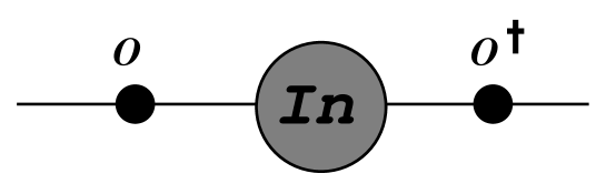
FIG. 10.: The one instanton contribution to $T\{{\cal O},{\cal O}^{\dagger}\}$.

Chay and Rey computed, in the dilute instanton gas approximation, the one instanton contribution to ${\rm d}\Gamma/{\rm d}y$ for $B\to X_{u}\ell\nu$ and $B\to X_{s}\gamma$ [15]. Their result diverges dramatically at the endpoint, as $y\to 1$. The contribution to $B\to X_{s}\gamma$ is nonetheless small and under control when one computes weighted spectra, but the same is not true for $B\to X_{u}\ell\nu$. Instead, one finds that the one instanton contribution is entirely untrustworthy in the experimentally defined window.

The one instanton contribution goes bad in this region presumably because multi-instanton configurations begin to be important. We have used the one instanton calculation as the motivation for a crude ansatz for the multi-instanton result in this region [16]. This ansatz incorporates, as much as possible, the reliable information from the one-instanton calculation. When we vary this naïve “best guess” ansatz by two orders of magnitude, we find that over most of the ansatz parameter space, the instantons do in fact dominate the weighted endpoint spectra.

One must be careful about interpreting this result. It is potentially interesting only in a negative sense. On the one hand, the actual numbers certainly cannot be believed; by no means do we claim to have computed the correct multi-instanton contribution. On the other, we have failed to find any justification for ignoring the instantons in the endpoint region. In light of this equivocal situation, one may well wonder whether one can still trust the relationship between the endpoint spectra for $B\to X_{s}\gamma$ and $B\to X_{u}\ell\nu$ proposed in Refs. [6, 7]. This is a situation badly in need of clarification. Invocations of faith, one way or the other, will not be sufficient; a more sophisticated estimate of instanton contributions is what is required. Such an estimate could show, for example, that our ansatz for the multi-instanton contribution is entirely too crude, and that other techniques can be used to prove that the multi-instanton contribution is necessarily negligible. We certainly hope that this will prove to be the case.

Conclusions

We may summarize the status of the theory of rare $B$ decays from each of our two viewpoints:

Low Energy Viewpoint:

1. Exclusive decay rates are extremely difficult to compute reliably. One must resort to models and other uncontrolled assumptions, a situation which is most unsatisfactory.

2. Inclusive calculations, by contrast, may be performed in a controlled expansion in powers of $\alpha_{s}$ and $1/m_{b}$. However, there remain unresolved uncertainties about

a. uncomputed higher orders in $\alpha_{s}$ and the renormalization scale $\mu$;

b. Sudakov double logarithms near the lepton energy endpoint;

c. instanton contributions near the lepton energy endpoint.

3. The decay $B\to X_{s}\gamma$ is in much better shape with respect to Sudakov and instanton corrections than is $B\to X_{u}\ell\nu$. Hence, while the calculation of $B\to X_{s}\gamma$ is itself perhaps fairly secure, the proposed relationship between the endpoint spectra in $B\to X_{s}\gamma$ and $B\to X_{u}\ell\nu$ may well be threatened by these effects.

High Energy Viewpoint:

1. In view of the significant uncertainties in existing theoretical calculations, only modifications to the Standard Model which affect rare decays at the $50\%$ level or higher are likely to be experimentally detectable. Small modifications, say at the $10\%$ level, are unlikely ever to be seen.

2. There is considerable room for the situation to improve, and much work remains to be done.

REFERENCES

- [1] M. Ciuchini, E. Franco, G. Martinelli, L. Reina and L. Silvestrini, Phys. Lett. B334, 137 (1994).
- [2] A. Buras, Nucl. Phys. B434, 606 (1995).
- [3] For reviews and references to the original literature, see N. Isgur and M.B. Wise, “Heavy Quark Symmetry,” in Decays, ed. S. Stone, Singapore: World Scientific, 1991, p. 158; B. Grinstein, 1994 TASI Lectures, UCSD Report No. USCD/PTH 94-24; M. Neubert, Phys. Rep. 245, 359 (1994).
- [4] J. Chay, H. Georgi and B. Grinstein, Phys. Lett. B247, 399 (1990); I.I. Bigi, N.G. Uraltsev and A.I. Vainshtein, Phys. Lett. B293, 430 (1992); I.I. Bigi, B. Blok, M. Shifman, N.G. Uraltsev and A.I. Vainshtein, Minnesota Report No. TPI–MINN–92/67–T (1992); A.F. Falk, M. Luke and M.J. Savage, Phys. Rev. D49, 3367 (1994).
- [5] A.V. Manohar and M.B. Wise, Phys. Rev. D49, 1310 (1994); I.I. Bigi, M. Shifman, N.G. Uraltsev and A.I. Vainshtein, Phys. Rev. Lett. 71, 496 (1993); B. Blok, L. Koyrakh, M. Shifman and A.I. Vainshtein, Phys. Rev. D49, 3356 (1994); Erratum, Phys. Rev. D50, 3572 (1994); T. Mannel, Nucl. Phys. B413, 396 (1994).
- [6] M. Neubert, Phys. Rev. D49, 3392 (1994); M. Neubert, Phys. Rev. D49, 4623 (1994); T. Mannel and M. Neubert, CERN Report No. CERN-TH-7156-94 (1994); I.I. Bigi, M. Shifman, N.G. Uraltsev and A.I. Vainshtein, Int. J. Mod. Phys. A9, 2467 (1994).
- [7] A.F. Falk, E. Jenkins, A.V. Manohar and M.B. Wise, Phys. Rev. D49, 4553 (1994).
- [8] A.F. Falk and M. Neubert, Phys. Rev. D47, 2965 (1993).
- [9] B. Guberina, R.D. Peccei and R. Rückl, Nucl. Phys. B171, 333 (1980).
- [10] S.J. Brodsky, G.P. Lepage and P.B. Mackenzie, Phys. Rev. D28, 228 (1983).
- [11] M. Luke, M.J. Savage and M.B. Wise, Phys. Lett. B343, 329 (1995).
- [12] M. Neubert, CERN Report Nos. CERN-TH-7487-94 (1994), CERN-TH-7524-94 (1995).
- [13] V. Sudakov, JETP (Sov. Phys.) 3, 65 (1956); G. Altarelli, Phys. Rep. 81, 1 (1982).
- [14] M Jeżabek and J.H. Kühn, Nucl. Phys. B320, 20 (1989).
- [15] J. Chay and S.J. Rey, Seoul Report Nos. SNUTP-94-08 (1994), SNUTP-94-54 (1994).
- [16] A.F. Falk and A. Kyatkin, Johns Hopkins Report No. JHU–TIPAC–950005 (1995).