hep-ph/9503473

Quark structure of the pion and pion form factor
V.Anisovich, D.Melikhov , and V.Nikonov
St.Petersburg Institute of Nuclear Physics, Gatchina, 188350, Russia

We consider the pion structure in the region of low and moderately high momentum transfers: at low $Q^{2}$, the pion is treated as a composite system of constituent quarks; at moderately high momentum transfers, $Q^{2}=10\div 25\;GeV^{2}$, the pion form factor is calculated within perturbative QCD taking into account one–gluon hard exchange. Using the data on pion form factor at $Q^{2}<3\;GeV^{2}$ and pion axial–vector decay constant, we reconstruct the pion wave function in the soft and intermediate regions. This very wave function combined with one–gluon hard scattering amplitude allows a calculation of the pion form factor in the hard region $Q^{2}=10\div 25\;GeV^{2}$. A specific feature of the reconstructed pion wave function is a quasi–zone character of the $q\bar{q}$–excitations. On the basis of the obtained pion wave function and the data on deep inelastic scattering off the pion, the valence quark distribution in a constituent quark is determined.

1 Introduction

Perturbative QCD gives rigorous predictions for exclusive amplitudes, in particular form factors at asymptotically large values of $Q^{2}$ [1]. For the pion form factor defined as

$$<\pi(P^{\prime})|J_{\beta}|\pi(P)>=(P^{\prime}+P)_{\beta}F_{\pi}(Q^{2})$$ (1)

the pQCD result takes the form

$$F_{\pi}(Q^{2})=8\pi f^{2}_{\pi}\frac{\alpha_{s}(Q^{2})}{Q^{2}}\left({1+\sum\limits_{N=2,4,...}C_{N}\left({{\rm ln}\frac{Q^{2}}{\mu^{2}}}\right)^{-\gamma_{N}}}\right)+O(1/Q^{4}).$$ (2)

Here $\gamma_{N}$ are the known positive numbers calculated within pQCD, $\mu$ is a constant about 1 $GeV$ dividing the perturbative and nonperturbative regions; $f_{\pi}=130\;MeV$ is the pion axial–vector decay constant, and the $C_{N}$ are expressed through the soft-region nonperturbative wave function of the pion. In the series (2), the contribution of diagrams with internal lines having virtualities above $\mu$ are taken into account perturbatively, while all the exchanges with lower virtualities are absorbed into the set of soft nonperturbative wave functions of the pion Fock components. The terms of the order $1/Q^{2}$ come only from the valence quark–antiquark component of the pion Fock state, whereas other components give the terms $O(1/Q^{4})$. The series (2) involves both the leading and subleading logarithms. In the leading logaithmic approximation (LLA) the expression (2) can be rewritten in the form

$$F_{\pi}(Q^{2})=\int_{0}^{1}dx\,dx^{\prime}\phi_{\pi}(x,Q^{2})T_{B}(x,x^{\prime},Q^{2})\phi_{\pi}(x^{\prime},Q^{2})$$ (3)

where $\phi(x,Q^{2})$ is the leading twist wave function (distribution amplitude) which describes the longitudinal momentum distribution of valence quark–antiquark pair whose relative transverse momentum is less than $Q$, and

$$T_{B}(x,x^{\prime},Q^{2})\to\frac{8\pi}{9}\frac{\alpha_{s}(xx^{\prime}Q^{2})}{xx^{\prime}Q^{2}}$$ (4)

is the amplitude of the hard interaction of the two free quarks in the Born approximation (Fig.1a).

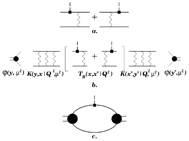
Figure 1: a. Hard scattering amplitude for two free quarks in the Born approximation. b. Hard scattering process in the LLA. c. Soft form factor.

The distribution amplitude at large $Q$ is related to the soft pion distribution amplitude $\phi_{\pi}(x,\mu^{2})$ by the gluon ladder evolution kernel $K(x,y,Q^{2}/\mu^{2})$ as follows

$$\phi_{\pi}(x,Q^{2})=\int K(x,y,Q^{2}/\mu^{2})\phi_{\pi}(y,\mu^{2})\,dy$$ (5)

The soft distribution amplitude is connected with the pion axial vector decay constant via the relation

$$\int\phi_{\pi}(x,\mu^{2})\;dx=f_{\pi},\quad f_{\pi}=130\;MeV$$ (6)

So, in the LLA hard scattering off the pion described by the expressions (3) and (5) (see Fig.1b) has a clear physical interpretation within the hard scattering picture [2], namely: The initial pion transforms into quark–antiquark pair with a small relative transverse momentum $\leq\mu$ and the longitudinal momentum fractions $x$ and $1-x$, respectively: this stage is described by $\phi(y,\mu^{2})$. Next, the quarks are coming closer to each other to the distances $1/Q$ and increase their virtualities via ladder gluon exchanges, described by $K$. Then, the hard interaction of almost free quarks with the external current occurs ($T_{B}$), and inverse evolution to low virtualities ($K$) with a subsequent pion formation ($\phi(y^{\prime},\mu^{2})$). A rigorous QCD result is that any soft distribution amplitude evolves at large $Q^{2}$ to the universal function

$$\phi^{as}_{\pi}(x)=\phi_{\pi}(x,Q^{2}\to\infty)=6f_{\pi}\,x\,(1-x).$$ (7)

Substituted into (3), this function gives the leading term in (2).

Unfortunately, this beautiful picture does not work at momentum transfers accessiblle to present–day experiments: the momentum transfers are not large enough. Trying to adjust this perturbative calculations for moderately high momentum transfers, Chernyak and Zhitnitsky [3] assumed the logarithmic and power corrections (including a purely soft contribution shown if Fig.1) to the Born term to be not essential, and the pion form factor to be described by

$$F_{\pi}(Q^{2})=\int_{0}^{1}dx\,\phi_{\pi}(x,\mu^{2})T_{B}(x,x^{\prime},Q^{2})dx^{\prime}\,\phi_{\pi}(x^{\prime},\mu^{2})$$ (8)

with $T_{B}$ still given by (4), but some modified distribution amplitude $\phi_{\pi}$. Describing the available pion form factor data by the formula (8), they came to the soft distribution amplitude of the form

$$\phi^{cz}_{\pi}(x,\mu\approx 0.5GeV)=30f_{\pi}x(1-x)(1-2x)^{2}$$ (9)

However, arguments against such an approach were put forward by Isgur and Llewellin Smith [4]. The problem is that the wave function of the form (9) strongly emphasizes the end-point region of $x\approx 0$ which was estimated to give $70\div 90\%$ of pion form factor at $Q^{2}=10\;GeV^{2}$. Recall that only the exchanges with virtualities above $\mu^{2}$ were considered perturbatively, otherwise the corresponding subprocesses were referred to the soft wave function. In the end–point region at moderately high $Q^{2}$, the gluon virtuality $xx^{\prime}Q^{2}$ is not large enough to justify the perturbative treatment. Hence, the end–point contribution should be rather referred to the nonperturbative one. The large contribution coming from small $x$ means that in fact the wave function with strongly emphasized end points has picked up a good portion of the nonperturbative contribution. So the latter turns out to be not small that contradicts to the inital assumption.

The arguments of [4] were supported by by recent applications of QCD sum rules [5],[6]: the end-point contribution remains numerically important at least up to $Q^{2}\approx 10\;GeV^{2}$, although parametrically it is suppressed by an extra power of $1/Q^{2}$. The problem of a correct extraction of the end–point contribution to hard scattering amplitudes was studied by Li and Sterman [7] and Radyushkin [8]. Their results give additional arguments against the application of the strategy of ref.[3] to hadron form factors at intermediate momentum transfers.

In addition, some problems are encountered when wave functions with an emphasized end–point region are applied to deep inelastic scattering. It was discussed [9] that the valence quark contribution to the deep inelastic structure function calculated with such distribution amplitudes exceeds the available data at large $x$, whereas there should be a room for other Fock components.

The attempts to describe the pion form factor in the region $Q^{2}=3\div 10\;GeV^{2}$ taking into account only the perturbative hard scattering mechanism were not successful. The nonperturbative contribution in this region is obviously not small. Our goal is to consider the pion form factor at moderately large $Q^{2}$ allowing for both the perturbative and nonperturbative contributions starting with low $Q^{2}$ and advancing to higher values.

Investigations of soft hadron processes in past decades have demonstrated constituent quarks to be relevant objects for describing hadron structure [10][11].

The nonperturbative contribution to the pion form factor was considered within the framework of the QCD-inspired constituent quark model ([12][13] [14][15][16]), the pion form factor being represented by the diagram of Fig.1c.

In the approach suggested here, we move to the region of large $Q^{2}$ starting with small values. That is, we take into account the diagram of Fig.2a and, as the following step, the diagrams of Figs.2b,c. The diagrams of Fig.2b and Fig.2c correspond to the terms with the minimal $N=0$ in the series (2). In fact, we recast the series (2) for the pion form factor as a series over $\alpha_{s}$. Such an expansion is relevant at moderately large $Q^{2}$.

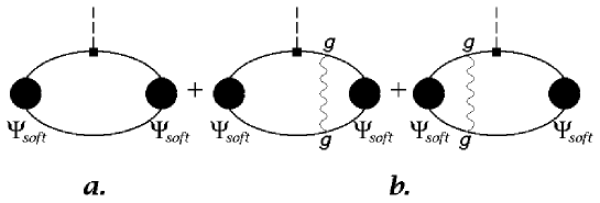
Figure 2: The expansion of the pion form factor in the series over $g^{2}$.

To be more quantitative, the procedure is as follows. The expansion for the pion form factor in a series over $\alpha_{s}$ reads

$$J^{\beta}(0)=[\bar{q}(0)\gamma^{\beta}q(0)]_{\mu^{2}}+\alpha_{s}\int dz_{1}dz_{2}[\bar{q}(0)q(z_{1})]_{\mu^{2}}|0>T^{\beta}_{B}(z_{1},z_{2})<0|[\bar{q}(z_{2})q(0)]_{\mu^{2}}+O(\alpha^{2}_{s})$$ (10)

To make this expansion meaningfull, the operator product expansion was performed, i.e. all the field operators were decomposed into soft and hard components. The subscript $\mu^{2}$ implies that the subdiagrams for corresponding operators involve only lines with virtualities below $\mu^{2}$. The contribution of the region of virtualities below $\mu^{2}$ is described by the soft wave functions, whereas the contribution of larger virtualities is represented by the hard scattering block $T_{B}$ [1].

Let us denote the corresponding contributions of the first and second terms in the r.h.s. of (10) as $F^{ss}$ (Fig.2a) and $2F^{sh}$ (Figs.2b,c), respectively. Then one finds

$$F_{\pi}=F^{ss}+2F^{sh}+O(\alpha^{2}_{s}).$$ (11)

The last series actually corresponds to dividing the pion light–cone wave function $\Psi$ into two parts such that $\Psi_{soft}$ is large at $s=\frac{m_{\perp}^{2}}{x(1-x)}<s_{0}$ while $\Psi_{hard}$ prevails at $s>s_{0}$. We perform such a decomposition of the wave function using the simplest ansatz with the step–function:

$$\Psi=\Psi_{soft}\theta(s_{0}-s)+\Psi_{hard}\theta(s-s_{0})$$ (12)

According to (10), $\Psi_{hard}$ is represented as a convolution of the one-gluon exchange kernel $V^{\alpha_{s}}$ with $\Psi_{soft}$

$$\Psi_{hard}=V^{\alpha_{s}}\otimes\Psi_{soft}.$$ (13)

The soft–soft contribution $F^{ss}$ in (11) is the usual quantity calculated within constituent quark models, whereas the soft–hard term $F^{sh}$ relates to the one given by the hard scattering mechanism. The soft–soft contribution includes the Sudakov form factor of the quark.
We obtain the following results:
(i) The pion form factor calculated in the region of $Q^{2}$ from 0 to 20 $GeV^{2}$ describes well the available data (Fig.3). The soft–soft contribution is found to give more than a half of the form factor in the region $Q^{2}\leq 20\;GeV^{2}$ and is not negligible up to $Q^{2}\leq 30\;GeV^{2}$. However, the particular numbers depend on how we define the boundary of the soft and the hard regions. We assume an extended soft region for $s\leq 9\;GeV^{2}$, that yields a large contribution of the soft–soft form factor until very high momentum transfers.
The transverse motion in the soft–hard term turns out to be important. At the same time, the Sudakov suppression is not large in the kinematical region of momentum transfers where the soft–soft term dominates.
(ii) The soft pion wave function which has been a variational quantity of our consideration is found to have a quasi–zone structure: it is large at low $s\leq 2\;GeV^{2}$, then it almost vanishes at $2\;GeV^{2}\leq s\leq 4.5\;GeV^{2}$, and has a bump at $4.5\;GeV^{2}\leq s\leq 9\;GeV^{2}$ (Fig.5).
(iii) The pion structure function is expressed through pion soft wave function and constituent quark structure function. By describing the data on pion valence quark $x$–distribution, we find the parameters of the $x$–distribution of valence quark inside a constituent quark to be in a qualitative agreement with Reggeized QCD–gluon intercept calculation [22].

The paper is organized as follows:
The Section 2 considers the pion as quark-antiquark bound state within the light–cone technique [17] reformulated as dispersion relation integrals and presents the expressions for the pion form factor and and quark distribution in deep inelastic scattering. All necessary technical details relevant to pion description are given in the Appendices. The results are discussed in the Section 3. A brief summary and outlook are given in the Conclusion.

2 Pion form factor and structure function

The light–cone technique expressed in the form of the deispersion relation integrals [18] allows constructing relativistic and gauge invariant amplitude of the interaction of a composite system with an external vector field starting with low-energy constituent scattering amplitude (see the Appendix A). Two-particle $s$-channel interactions are consistently taken into account both in the constituent scattering amplitude and the amplitude of interaction with an external field. In the case of a bound state, its form factor and structure function are expressed through form factor and structure function of mass-shell constituents and the vertex $G$ of constituent–bound state transition. This vertex is defined by the two–particle irreducible block of the constituent scattering amplitude. On the one hand, the dispersion integral representation turns out to be equivalent to the Bethe–Salpeter treatment with a separable kernel of a special form, the vertex $G$ being connected with the amputated Bethe-Salpeter wave function of the bound state. On the other hand, this approach can be formulated as a light–cone description of a bound state with the special form of spin transformation (the Melosh rotation). Because of the relativistic invariance, the dispersion integral approach does not face the problem of choosing appropriate component of the current for form factor calculation. The function $G$ determines the bound–state light–cone wave function [18]. Note also that only amplitudes for on-shell constituents contribute to corresponding amplitudes of the bound state. This guarantees gauge invariance of the derived expressions and escapes the problem of constituent amplitudes off the mass shell. All relevant details can be found in the Appendix A.

Our position on the pion structure completely coincides with the viewpoint formulated by Weinberg [11]: Successes of the quark model allow one to treat quarks as usual massive hadrons with the only difference that quarks are subject to color forces which become essential at large distances and keep quarks confined in hadrons; in all other aspects these forces are weak and quarks can be treated as real particles.

In the soft region, quark structure of a pion is described by the vertex

$$\frac{\bar{Q}^{a}(P-k)i\gamma_{5}Q^{a}(k)}{\sqrt{N_{c}}}G_{v}(P^{2})$$ (14)

with $a$ a color index, $N_{c}=3$ the number of quark colors, $k^{2}=m^{2}$, $(P-k)^{2}=m^{2}$, but $P^{2}=s\neq m_{\pi}^{2}$. Here $m$ is a constituent quark mass. We consider $\pi^{+}$ and omit the flavor which gives the unity factor. (the appendix B presents a detailed consideration) The soft vertex $G_{v}$ is supposed to be nonzero at $s<s_{0}$ in accordance with (12). Once the vertex is fixed, we can proceed with form factor calculation.

2.1 Soft–soft contribution to pion form factor

The double dispersion relation integral for a soft–soft contribution to the pion form factor is given by the following expression

$$F^{ss}(q^{2})=\int\frac{ds\;G_{v}(s)}{\pi(s-M^{2})}\frac{ds^{\prime}G_{v}(s^{\prime})}{\pi(s^{\prime}-M^{2})}\Delta_{\pi}(s^{\prime},s,q^{2})f_{c}(q^{2}).$$ (15)

Here $f_{c}$ is a constituent form factor, $f_{c}(0)=1$. The quantity $\Delta_{\pi}$ is defined as follows

$$-\frac{1}{8\pi}\int dk_{1}dk^{\prime}_{1}dk_{2}\delta(k^{2}_{1}-m^{2})\delta(k^{\prime 2}_{1}-m^{2})\delta(k^{2}_{2}-m^{2})\delta(P-k_{1}-k_{2})\delta(P^{\prime}-k^{\prime}_{1}-k_{2})$$

$$\times Sp\left({(\hat{k}^{\prime}_{1}+m)\gamma_{\mu}(\hat{k}_{1}+m)i\gamma_{5}(m-\hat{k}_{2})i\gamma_{5}}\right)=2P_{\mu}(q)\Delta_{\pi}(s^{\prime},s,q^{2})$$ (16)

with

$$P_{\mu}(q)=(P-\frac{qP}{q^{2}}\,q)_{\mu},\;P^{2}=s,\;P^{\prime 2}=s^{\prime},\;(P^{\prime}-P)^{2}=q^{2}.$$

The trace reads

$$\frac{1}{4}Sp\left({(\hat{k}^{\prime}_{1}+m)\gamma_{\mu}(\hat{k}_{1}+m)\gamma_{5}(m-\hat{k}_{2})\gamma_{5}}\right)=m^{2}(k_{1}+k^{\prime}_{1})_{\mu}+k_{1\mu}(k^{\prime}_{1}k_{2})+k^{\prime}_{1\mu}(k_{1}k_{2})-k_{2\mu}(qk_{1})$$ (17)

To reveal the relationship between the dispersion integral (15) and the lihgt–cone technique, we introduce the light–cone variables

$$k_{-}=\frac{1}{\sqrt{2}}(k_{0}-k_{z});\quad k_{+}=\frac{1}{\sqrt{2}}(k_{0}+k_{z});\quad k^{2}=2k_{+}k_{-}-k^{2}_{\perp};$$ (18)

into the representation (16) and use the reference frame

$$q_{+}=0,\qquad P_{\perp}=0,\qquad q^{2}=-q^{2}_{\perp}<0,$$ (19)

The form factor takes the form

$$F^{ss}(q^{2}_{\perp})=\frac{1}{\pi}\int dxd^{2}k_{\perp}\psi(x,k_{\perp})\psi(x,k_{\perp}-xq_{\perp})\beta(x,k_{\perp},q_{\perp})f_{c}(q^{2}_{\perp}),$$ (20)

where the soft radial light-cone wave function of a pion is introduced

$$\psi(x,k_{\perp})=\frac{G_{v}(s)\sqrt{s}}{\pi\sqrt{8}(s-m^{2}_{\pi})\sqrt{x(1-x)}},\qquad s=\frac{m^{2}+k^{2}_{\perp}}{x(1-x)}$$ (21)

$$\beta=\frac{m^{2}+k^{2}_{\perp}-xk_{\perp}q_{\perp}}{\sqrt{m^{2}+k^{2}_{\perp}}\;\sqrt{m^{2}+(k_{\perp}-xq_{\perp})^{2}}}.$$

The quantity $\beta$ accounts for the contribution of spins. It is different from unity at $q_{\perp}\neq 0$ because both the nonspin-flip and spin-flip amplitudes of the interacting quark contribute. The relation $F_{\pi}(0)=1$ is the normalization condition for the soft radial wave function

$$\int dx\;dk^{2}_{\perp}\;|\psi(x,k_{\perp})|^{2}=1.$$ (22)

The pion axial–vector decay constant $f_{\pi}$ related to the $\pi\to\mu\nu$ decay is given by

$$g_{A}\frac{\sqrt{N_{c}}}{\sqrt{2}\pi}\int{dx\;dk^{2}_{\perp}}\frac{m}{\sqrt{m^{2}+k^{2}_{\perp}}}\;\psi(x,k_{\perp})={f_{\pi}}$$ (23)

where $g_{A}$ is the constituent quark axial–vector coupling constant. From the analysis of the neutron $\beta$–decay within various models, the value of $g_{A}$ was found to be in the range from 0.75 (nonrelativistic constituent quark model without configuration mixing in the nucleon wave function, $m\approx 0.33\;GeV$) up to 1.0 (relativistic quark model with light constituent quarks, $m\approx 0.25\;GeV$ [15].) Here we use the relation (23) to fix the value of $g_{A}$ related to a particular pion wave function such that (23) reproduces the observed value $f_{\pi}=130\;MeV$. The value of $g_{A}$ is found to lie in the range $g_{A}\approx 0.75\div 1$ (see the Table 1).

The same expressions for the form factor and pion electroweak constant as (20)–(23) were derived in refs [14]–[16]. In contrast to the mentioned papers where such formulas were applied to describing the total pion form factor , we use them for calculating the soft–soft contribution.

The soft-soft form factor involves the constituent quark form factor which should satisfy the conditions $f_{c}(0)=1$ and $f_{c}(Q^{2})\to S(Q^{2})$ at large $Q^{2}=-q^{2}$. Here $S(Q^{2})$ is the Sudakov form factor which is taken in the form [8]

$$S(Q^{2})={\rm exp}\left({-\frac{\alpha_{s}(Q^{2})}{2\pi}C_{F}{\rm log}^{2}\left({\frac{Q^{2}}{Q^{2}_{0}}}\right)}\right),\;C_{F}=\frac{N_{c}^{2}-1}{2N_{c}}=\frac{4}{3},\;Q_{0}\approx 0.85\div 1\;GeV$$ (24)

with $\alpha_{s}$ the coupling constant. At low $Q^{2}$ we assume $\alpha_{s}$ to be frozen at $1\;GeV^{2}$, namely we set

$$\alpha_{s}(Q^{2}) = \frac{4\pi}{9}{\rm log}^{-1}\left({\frac{Q^{2}}{\Lambda^{2}}}\right),\;\Lambda=0.22\;GeV,\quad Q^{2}<1\;GeV^{2}$$ (25)

$$= {\rm const,}\quad Q^{2}<1\;GeV^{2}$$

The constituent quark form factor is taken as

$$f_{c}(Q^{2}) = 1,\;Q<Q_{0}$$

$$= S(Q^{2}),\;Q>Q_{0},\;S(Q_{0}^{2})=1$$

Note that the Sudakov suppression is absent in the soft-hard term.

2.2 Soft–hard contribution to the pion form factor

In accordance with (10), the soft–hard contribution is described by the two graphs of Fig.2b,c with one–gluon exchanges. The corresponding dispersion relation integral reads

$$F^{sh}=\int\frac{ds\;G_{v}(s)\;\theta(s<s_{0})}{\pi(s-m^{2}_{\pi})}\frac{ds^{\prime\prime}\theta(s^{\prime\prime}>s_{0})}{\pi(s^{\prime\prime}-m^{2}_{\pi})}D(s,s^{\prime\prime},s^{\prime},q^{2})\frac{ds^{\prime}\;G_{v}(s^{\prime})\;\theta(s^{\prime}<s_{0})}{\pi(s^{\prime}-m^{2}_{\pi})}$$ (27)

In this expression, $D(s,s^{\prime\prime},s^{\prime},q^{2})$ is a spectral density which takes into account the one-gluon exchange at large $s^{\prime\prime}$; the Appendix C presents the details of the soft–hard form factor $F^{sh}$ calculation. Notice that the dispersion expression involves only two–particle singularities and neglects three–particle intermediate state related to cutting the gluon line. The final result has the form

$$F^{sh}(q_{\perp}^{2})=\frac{C_{F}}{8\pi}\int\frac{dxd^{2}k_{\perp}}{\pi\sqrt{m^{2}+k^{2}_{\perp}}(1-x)}\psi(x,k_{\perp})\theta(s<s_{0})\frac{\theta(s^{\prime\prime}>s_{0})}{\frac{m^{2}+(k_{\perp}-xq_{\perp})^{2}}{x(1-x)}-m^{2}_{\pi}}$$ (28)

$$\times\frac{dx^{\prime}d^{2}k^{\prime}_{\perp}}{\sqrt{m^{2}+(k^{\prime}_{\perp}-x^{\prime}q_{\perp})^{2}}}\psi(x^{\prime},k^{\prime}_{\perp}-x^{\prime}q_{\perp})\theta(s^{\prime}<s_{0})Tr(s,s^{\prime},s^{\prime\prime},q^{2})\frac{\alpha_{s}\left({-(k-k^{\prime})^{2}}\right)}{m_{G}^{2}-(k^{\prime}-k)^{2}}$$

where

$$-(k^{\prime}-k)^{2}=\frac{(k^{\prime}_{\perp}x-k_{\perp}x^{\prime})^{2}+m^{2}(x-x^{\prime})^{2}}{xx^{\prime}},$$

$$Tr(s,s^{\prime},s^{\prime\prime},q^{2})=2s^{\prime}\left({\alpha(s^{\prime\prime},s,q^{2})(s^{\prime\prime}+s-q^{2})+q^{2}}\right)-4m^{2}\left({\alpha(s^{\prime\prime},s,q^{2})(s^{\prime}+s-q^{2})+q^{2})}\right);$$

$$\alpha(s^{\prime\prime},s,q^{2})=\frac{-q^{2}(s^{\prime\prime}+s-q^{2})}{(s^{\prime\prime}-s)^{2}-2q^{2}(s^{\prime\prime}+s)+q^{4}}$$

and

$$s=\frac{m^{2}+k_{\perp}^{2}}{x(1-x)},\quad s^{\prime\prime}=\frac{m^{2}+(k_{\perp}-xq_{\perp})^{2}}{x(1-x)},\quad s^{\prime}=\frac{m^{2}+(k^{\prime}_{\perp}-x^{\prime}q_{\perp})^{2}}{x^{\prime}(1-x^{\prime})}$$

In (28) $m_{G}$ is the gluon mass which depends on the gluon momentum squared $-(k^{\prime}-k)^{2}$ and is normalized to be of the order of $1\;GeV$ in the soft region [19].
One can easily see that $F^{sh}(0)=0$.
Let us turn to the region of large $Q^{2}$ and compare the soft–hard term which dominates the form factor with the standard pQCD expression (3) and (4). Using the relations

$$Tr\to 4m^{2}Q^{2}x\qquad{\rm and}\qquad-(k^{\prime}_{2}-k_{2})^{2}\to xx^{\prime}Q^{2}$$

we find

$$F_{\pi}(Q^{2})\to\frac{1}{\kappa^{2}}\int\;\phi(x,s_{0})\;dx\frac{8\pi}{9}\frac{\alpha_{s}(xx^{\prime}Q^{2})}{xx^{\prime}Q^{2}}\phi(x^{\prime},s_{0})\;dx^{\prime}$$ (29)

Here we introduced the distribution amplitude $\phi(x,s_{0})$ normalized by the standard condition

$$\int\phi(x,s_{0})\;dx=f_{\pi}$$ (30)

This distribution amplitude is related to the soft radial wave function (21) via the relation

$$\phi(x,s_{0})=\frac{\sqrt{N_{c}}\kappa}{\sqrt{2}\pi}\int dk_{\perp}^{2}\frac{m}{\sqrt{m^{2}+k_{\perp}^{2}}}\psi(x,k_{\perp})\theta\left({\frac{m^{2}+k_{\perp}^{2}}{x(1-x)}<s_{0}}\right)$$ (31)

The expression (21) differs from (8) by the factor $1/\kappa^{2}$, where

$$\kappa=g^{0}_{A}(0)=0,75\div 1$$ (32)

(see the eq.(78) of the Appendix B) is the axial–vector decay constant at the level of a constituent quark. If we identify constituent quarks with a bare pQCD quarks, then $g^{0}_{A}=1$. Here we assume such an identification to be not well–justified in the region $Q^{2}\leq 10\;GeV^{2}$ and hence we allow $\kappa$ to be in the range from 0.75 to 1.

Actually, a constituent quark is a Fock state involving the components $q_{val},q_{val}\bar{q}q,q_{val}\bar{q}qg,\ldots$ At asymptotically large momentum transfers only the valence component survives whereas all other components do not contribute to the form factor. The problem of the typical $Q$ at which the transfer to the asymptotic regime occurs is still opened. It is quite natural that the expression (29) gives a larger value for the form factor at $\kappa<1$ since it includes the contribution of all higher Fock components of the constituent quark in addition to the valence one.

2.3 Structure function

Now we have all necessary to calculate the pion structure function $F_{2}(x)$. This function is given by the convolution of the pion light–cone soft wave function and the corresponding constituent quark structure function $f^{i}_{2}(x)$

$$F_{2}(x,Q^{2})=\sum\limits_{j=Q,\bar{Q}}\int_{x}^{1}dk^{2}_{\perp}dx^{\prime}\psi(x^{\prime},k_{\perp})^{2}f^{j}_{2}\left({\frac{x}{x^{\prime}},Q^{2}}\right)$$ (33)

The leading order expressions for these structure functions in terms of parton densities read

$$F_{2}(x)=\sum\limits_{flavours}e_{i}^{2}x\;Q_{i}(x),\quad f^{j}_{2}(x)=\sum\limits_{flavours}e_{i}^{2}x\;q^{j}_{i}(x)$$ (34)

where $Q_{i}$ and $q^{j}_{i}$ are quark parton densities of a given flavour $i$ inside a pion and constituent quark $j$, respectively.

At large $x$ the behavior of the structure functions is determined by the valence quark (antiquark) distribution $v(x)$ inside the constituent quark (antiquark). The latter is taken in the form

$$v(x)\approx x^{-a}(1-x)^{-b}\left({1-N(1-x)^{c}}\right)$$ (35)

The parameters in this formula are chosen such that $v(x)$ should satisfy the following sum rules at $Q_{0}^{2}=10\;GeV^{2}$

$$\int\limits_{0}^{1}v(x,Q_{0}^{2})dx=1\qquad\int\limits_{0}^{1}v(x,Q_{0}^{2})xdx=0.35$$ (36)

The last number is the fraction of constituent quark momentum carried by the valence quark. Due to the sum rule for momentum, this value is equal to the fraction of hadron momentum carried by valence quarks. For a proton this fraction is known to be $\approx 0.35$ at $10\;GeV^{2}$.

3 The results of fitting the data on form factor and deep inelastic parton distribution

Fig.3 shows the results of fitting the data on $F_{\pi}(Q^{2})$ [20] via the formulas (20) and (21) for $F^{ss}$ and (28) for $F^{sh}$. Fig.3a demonstrates the region of low $Q^{2}$ where $F^{ss}$ dominates; Fig.3b emphasizes the region of moderately large $Q^{2}$, $Q^{2}=5\div 20\;GeV^{2}$. Fig.4 plots the typical contribution of the soft–hard term to the pion form factor. Several variants of the calculation relate to different sets of the parameters $m_{G},\alpha_{s}$, and $m$ presented in the Table 1. Let us point out that $g_{A}^{0}$ calculated with the determined wave function appreciably depends on the constituent quark mass: for a heavy constituent quark $g^{0}_{A}$ is rather small and equal to 0.86, whereas for a light constituent quark $g^{0}_{A}$ is close to unity.

In all the fits the soft pion wave function $\psi(x,k^{2}_{\perp})$ was the basic variational quantity. Fig.5 presents the typical reconstructed soft wave function. A specific feature of the reconstructed wave function is a quasi–zone character of $\bar{q}q$–excitations in the pion. We tried to find a parametrization without a dip in the region $2\div 4\;GeV^{2}$ but failed; all the used fitting procedures suggested qualitatively similar double–humped wave functions. So one can think this dip to reflect some essential feature of the $\bar{q}q$ dynamics inside the pion. However, we have no definite ideas on the origin of such a specific behavior.

Fig.6 displays the distribution amplitude $\phi(x)$ calculated with the determined $G_{v}(s)$. It turned out to be very close to the asymptotic function (7).

Fig.7 presents the valence quark distribution inside the pion. The parameters of the distribution (35) $b=0.99$ and $a$ and $c$ from the range $a=0.5\div 0.7$ and $c=1\div 2$ were found to provide a reasonable description of the data [21]. Mention that $b$ is very close to unity. If the valence quark distribution is determined by the Reggeized–gluon exchange, then our result gives for its intercept the value close to unity in qualitative agreement with [22].

Table 1: Table of the parameters in the pion form factor calculations. We assumed $m_{G}(\kappa^{2})=m_{G}^{0}(1-\kappa^{2}/0.5)$ as $\kappa^{2}<0.5\;GeV^{2}$ and $m_{G}=0$ as $\kappa^{2}>0.5\;GeV^{2}$, where $\kappa$ is the gluon momentum.

	Set 1	Set 2	Set 3	Set4
constituent quark mass $m$, GeV	0.35	0.35	0.35	0.35
$m_{G}^{0}$, GeV	0.7	0.7	0	0
$\alpha_{s}$ in (28)	$\alpha_{s}(Q^{2}/4)$	$\alpha_{s}(\kappa^{2})$	$\alpha_{s}(Q^{2}/4)$	$\alpha_{s}(\kappa^{2})$
$g_{A}(0)$	0.86	0.86	0.86	0.86

Figure 3: The pion form factor. Solid line – calculations with the Set 1 of the parameters; dashed–dotted line – Set 2, dashed line – Set 3, dotted line – Set 4.

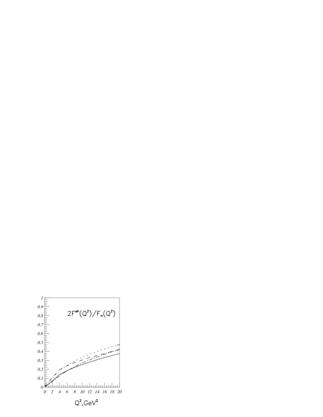
Figure 4: The contribution of the soft–hard term to the pion form factor. The curve notation is the same as for the form factor.

Figure 5: The soft light–cone wave function of the pion.

Figure 6: The distribution amplitude. Solid line – our calculation; dashed line – asymptotical curve $\phi(x)=6x(1-x)$.

Figure 7: Valence distribution in a pion $x\,V(x,Q^{2}=10\;GeV^{2})$. The solid curve – $a=0.69,\;b=0.99,\;c=1$; the dashed curve – $a=0.46,\;b=0.99,\;c=1.55$.

4 Conclusion

We have analyzed the pion structure within a dispersion relation formulation of the light–cone technique when the pion in the soft region is treated as a two constituent quark bound state. At small values of the $\bar{q}q$ light–cone energy the pion is described by a model soft wave function, whereas at large values the one–gluon hard exchange is taken into account. This provides the form factor high–$Q^{2}$ asymptotic behavior in agreement with pQCD. The obtained pion form factor describes well the available experimental data at $Q^{2}\div 10\;GeV^{2}$.
Our results are as follows:

• We considered the soft–soft ($F^{ss}$) and soft–hard ($2F^{sh}$) contributions to the pion form factor within the light–cone quantum mechanics. The derived expressions involve the soft radial wave function of the pion which has been treated as a variational parameter of the approach. By fitting the data on the pion form factor at $Q^{2}\leq 3\;GeV^{2}$, we determined this soft radial wave function. This allowed a calculation of the relative soft–hard contribution to the pion form factor in a broad range of momentum transfers. It turned out to be relatively small (less than 50% at $Q^{2}=20\;GeV^{2}$) because we used a large value for the boundary of light–cone energy squared dividing the soft and the hard regions ($s_{0}=9\;GeV^{2}$) and hence we related a large portion of the pion form factor to the soft–soft contribution. However, smaller values of this boundary do not change qualitatively the results, except for quantitative increasing the soft–hard fraction.
  The calculated pion axial–vector decay constant agrees well with the experimental value.

• The soft radial light–cone wave function as a function of the square of the light–cone $\bar{q}q$ energy $s$ has been found to demonstrate a specific behavior: it is large at $s\leq 2\;GeV^{2}$, close to zero as $s=2\div 4\;GeV^{2}$, and has a bump in the region $s=4\div 9\;GeV^{2}$. Our attempts to find a wave function of a more regular shape failed as all the fits suggested a double–humped behavior. We have no definite ideas about the origin of such a quasi–zone character of the $\bar{q}q$ excitations. Nevertheless, such an unexpected wave function seems to reflect some unknown essential details of the quark dynamics in the pion.

• The distribution amplitude $\phi(x)$ calculated with the obtained soft wave function turns out to be very close to the asymptotic function $\phi^{as}_{\pi}(x)$ predicted by pQCD.

• Describing the data on deep inelastic scattering off the pion allowed investing the parton structure of the constituent quark. The distribution of the valence quark–parton in the constituent quark is found to be in a qualitative agreement with the parametrization suggested by the Reggeized–gluon exchange.

The authors are grateful to the International Science Foundation for financial support under grant R1000.

5 Appendix A: Bound state description within dispersion relations

To illustrate main points of the dispersion approach we consider the case of two spinless constituents with the masses $m$ interacting via exchanges of a meson with the mass $\mu$. We start with the scattering amplitude

$$A(s,t)=<k^{\prime}_{1},k^{\prime}_{2}|S|k_{1},k_{2}>,\quad s=(k_{1}+k_{2})^{2},\;t=(k_{1}-k^{\prime}_{1})^{2}$$ (37)

The amplitude as a function of $s$ has the threshold singularities in the complex $s$-plane connected with elastic rescatterings of the constituents and production of new mesons at

$$s=4m^{2},\;(2m+\mu)^{2},\;(2m+2\mu)^{2}\ldots$$ (38)

We assume that an $S$-wave bound state with the mass $M<2m$ exists, then the partial amplitude $A_{0}(s)$ has a pole at $s=M^{2}$. The amplitude $A(s,t)$ has also $t$-channel singularities at $t=(n\mu)^{2};\;\;n=1,2,3\ldots$ connected with meson exchanges. If one needs to construct the amplitude in the low-energy region $s\geq 4m^{2}$ the dispersion $N/D$ representation turns out to be convenient. Consider the $S$-wave partial amplitude

$$A_{0}(s)=\int\limits^{1}_{-1}dz\,A(s,t(s,z)),$$ (39)

where $t(z)=-2(s/4\,-m^{2})(1-z)$, $z=\cos\theta$ in the c.m.s. The $A_{0}(s)$ as a function of complex $s$ has the right-hand singularities related to $s$-channel singularities of $A(s,t)$. In addition, it has left-hand singularities located at $s=4m^{2}-(n\mu)^{2};\;\;n=1,2,3\ldots$. They come from $t$-channel singularities of $A(s,t)$. The unitarity condition in the region $s\approx 4m^{2}$ reads

$${\rm Im}\,A_{0}(s)=\rho(s)\;|A_{0}(s)|^{2},\qquad\rho(s)=\frac{1}{16\pi}\sqrt{1-\frac{4m^{2}}{s}}$$ (40)

with $\rho(s)$ the two-particle phase space. The $N/D$ method represents the partial amplitude as $A_{0}(s)=N(s)/D(s)$, where the function $N$ has only left-hand singularities and $D$ has only right-hand ones. The unitarity condition yields

$$D(s)=1-\int\limits^{\infty}_{4m^{2}}\frac{d\tilde{s}}{\pi}\,\frac{\rho(\tilde{s})N(\tilde{s})}{\tilde{s}-s}\;\equiv\;1-B(s).$$ (41)

Assuming the function $N$ to be positive we introduce $G(s)=\sqrt{N(s)}$. Then the partial amplitude takes the form

$$A_{0}(s)=G(s)\left[1+B(s)+B^{2}(s)+B^{3}(s)+\ldots\right]G(s)=\frac{G(s)G(s)}{1-B(s)}.$$ (42)

This expression can be interpreted as a series of loop diagrams of Fig.8

Figure 8: One of the terms in the expansion of $A_{0}(s)$

with the basic loop diagram

$$B(s)=\int\limits^{\infty}_{4m^{2}}\frac{d\tilde{s}}{\pi}\,\frac{\rho(\tilde{s})\;G^{2}(\tilde{s})}{\tilde{s}-s}.$$ (43)

The bound state with the mass $M$ relates to a pole both in the total and partial amplitudes at $s=M^{2}$ so $B(M^{2})=1$. Near the pole one has for the total amplitude

$$A = <k^{\prime}_{1},k^{\prime}_{2}|P>\frac{1}{M^{2}-P^{2}}<P|k_{1},k_{2}>+{\rm regular\;terms}$$ (44)

$$\equiv \chi^{*}_{P}(k^{\prime}_{1},k^{\prime}_{2})\frac{1}{M^{2}-P^{2}}\chi_{P}(k_{1},k_{2})+\ldots$$

where $\chi_{P}(k_{1},k_{2})$ is the amputated Bethe-Salpeter amplitude of the bound state. The dispersion amplitude near the pole reads

$$A=N/D+{\rm regular\;terms\;related\;to\;other\;partial\;waves}$$

$$=\frac{G^{2}(M^{2})}{(M^{2}-s)B^{\prime}(M^{2})}+\ldots\equiv\frac{G_{v}^{2}(M^{2})}{M^{2}-s}+\ldots$$ (45)

where $G_{v}$ is a vertex of the bound state transition to the constituents. The singular terms correspond to each other and hence

$$\chi_{P}(k_{1},k_{2})\to G_{v}(P^{2})\equiv\frac{G(P^{2})}{\sqrt{B^{\prime}(M^{2})}}$$ (46)

Underline that among right-hand singularities the constructed dispersion amplitude takes into account only the two-particle cut.

Let us turn to the interaction of the two-constituent system with an external electromagnetic field. The amplitude of this process $T_{\mu}=<k^{\prime}_{1},k^{\prime}_{2}|J_{\mu}(q)|k_{1},k_{2}>$ in the case of a bound state takes the form

$$T_{\mu} = <k^{\prime}_{1},k^{\prime}_{2}|P^{\prime}>\frac{1}{P^{\prime 2}-M^{2}}<P^{\prime}|J_{\mu}(q)|P>\frac{1}{P^{2}-M^{2}}<P|k_{1},k_{2}>+\ldots$$ (47)

$$= \chi^{*}_{P}(k^{\prime}_{1},k^{\prime}_{2})\frac{1}{P^{\prime 2}-M^{2}}(P^{\prime}+P)_{\mu}F(q^{2})\frac{1}{P^{2}-M^{2}}\chi_{P}(k_{1},k_{2})+\ldots$$

where the bound state form factor is defined as

$$<P^{\prime}|J_{\mu}(q)|P>=(P^{\prime}+P)_{\mu}F(q^{2})$$ (48)

The dispersion amplitude $T_{\mu}$ with only two-particle singularities in the $P^{2}$- and $P^{\prime 2}$-channels taken into account is given [23] by the series of graphs in Fig.9.

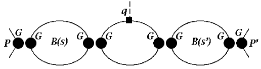
Figure 9: One of the terms in the series for $T_{\mu}$.

These graphs are obtained from the dispersion scattering amplitude series by inserting a photon line into constituent lines. The amplitude reads

$$T_{\mu}(P^{\prime},P,q)=2P_{\mu}(q)T(s^{\prime},s,q^{2})+\frac{q_{\mu}}{q^{2}}C,$$ (49)

$$P^{2}=s,\;P^{\prime 2}=s^{\prime},\;q=P^{\prime}-P,\;P_{\mu}(q)=(P-\frac{qP}{q^{2}}\,q)_{\mu}$$

The dispersion method allows one to determine $T(s,s^{\prime},q^{2})$, which is the part of the amplitude transverse with respect to $q_{\mu}$. Summing up the series of dispersion graphs in Fig.9 gives

$$T(s^{\prime},s,q^{2})=\frac{G(s)}{1-B(s)}\Gamma(s^{\prime},s,q^{2})\frac{G(s^{\prime})}{1-B(s^{\prime})}.$$ (50)

Here

$$\Gamma(s^{\prime},s,q^{2})=\int\frac{d\tilde{s}G(\tilde{s})}{\pi(\tilde{s}-s)}\frac{d\tilde{s}^{\prime}G(\tilde{s}^{\prime})}{\pi(\tilde{s}^{\prime}-s)}\Delta(\tilde{s}^{\prime},\tilde{s},q^{2}),$$

and $\Delta(\tilde{s}^{\prime},\tilde{s},q^{2})$ is the double spectral density of the three-point Feynman graph with a pointlike vertex of the constituent interaction.

The longitudinal part $C$ is given by the Ward identity

$$C=\frac{G(s)}{1-B(s)}\left({B(s^{\prime})-B(s)}\right)\frac{G(s^{\prime})}{1-B(s^{\prime})}$$ (51)

At $s=s^{\prime}=M^{2}$, the quantity $T_{\mu}$ develops both $s$ and $s^{\prime}$ poles, so

$$T_{\mu}(P^{\prime},P,q)=\frac{G_{v}(M^{2})}{M^{2}-s}(P^{\prime}+P)_{\mu}F(q^{2})\frac{G_{v}(M^{2})}{M^{2}-s^{\prime}}+{\rm less\;singular\;terms}$$ (52)

where

$$F(q^{2})=\int\frac{dsG_{v}(s)}{\pi(s-M^{2})}\frac{ds^{\prime}G_{v}(s^{\prime})}{\pi(s^{\prime}-M^{2})}\Delta(s^{\prime},s,q^{2}).$$ (53)

is the bound–state form factor (see (46) and (47)). So, the quantity $<P^{\prime}|J_{\mu}(q)|P>$ corresponds to the three–point dispersion graph with the vertices $G_{v}$. The following relation is valid $\Delta(s^{\prime},s,0)=\pi\delta(s^{\prime}-s)\rho(s)$. This is a consequence of the Ward identity which relates the three-point graph at zero momentum transfer to the loop graph. This relation yields the charge normalization $F(0)=1$. The expression (53) gives the form factor in terms of the $N$-function of the constituent scattering amplitude and double spectral density of the Feynman graph. In general, the following prescription works: to obtain the dispersion expression spectral density in channels corresponding to a bound state, one should calculate the related Feynman graph spectral density and multiply it by $G_{v}$.

Mention that only on-shell constituents contribute to all the quantities. If the constituent is a nonpoint particle, the expression (53) should be multiplied by form factor of an on-shell constituent.

6 Appendix B: Pion within the dispersion approach

We start with describing the quark-pion vertex. For on-shell quarks there is one independent structure $i\bar{q}^{a}\gamma_{5}q^{a}/\sqrt{N_{c}}$, with $a$ a color index and $N_{c}=3$ the number of quark colors. We consider a $\pi^{+}$ and omit the flavor which gives the unity factor. Let us introduce the momentum $P_{\pi}$, $P_{\pi}^{2}=m^{2}_{\pi}$. We shall also use an off-shell pion momentum $P$, $P^{2}=s$. The pionic dispersion loop graph Fig.10 reads

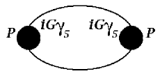
Figure 10: Pionic dispersion loop graph $B_{\pi}(P^{2})$.

$$B_{\pi}(P^{2})=\int\limits^{\infty}_{4m^{2}}\frac{ds\;G^{2}(s)}{\pi(s-P^{2})}\rho_{\pi}(s),\quad B_{\pi}(m^{2}_{\pi})=1$$ (54)

with $\rho_{\pi}(s)$ the spectral density of the Feynman loop graph

$$\rho_{\pi}(s)=-\frac{1}{8\pi^{2}}\int dk_{1}dk_{2}\delta(k^{2}_{1}-m^{2})\delta(k^{2}_{2}-m^{2})\delta(P-k_{1}-k_{2})\;Sp\left({(\hat{k}_{1}+m)i\gamma_{5}(m-\hat{k}_{2})i\gamma_{5}}\right)$$ (55)

$$=\frac{s}{8\pi}\sqrt{1-\frac{4m^{2}}{s}}\;\theta(s-4m^{2})$$

with $m$ a constituent quark mass.

The form factor of a pion is given by the following matrix element

$$<P^{\prime}_{\pi}|J^{em}_{\mu}(0)|P_{\pi}>=(P^{\prime}_{\pi}+P_{\pi})_{\mu}\;F_{\pi}(q^{2})$$ (56)

$$P^{2}_{\pi}=P^{\prime 2}_{\pi}=M^{2},\;(P^{\prime}_{\pi}-P_{\pi})^{2}=q^{2}.$$

The double dispersion representation for the form factor corresponds to Fig.11

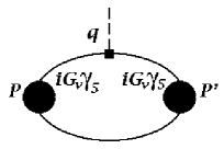
Figure 11: The soft–soft contribution $F^{ss}_{\pi}(q^{2})$ to pion form factor.

$$F_{\pi}(q^{2})=\int\frac{ds\;G_{v}(s)}{\pi(s-M^{2})}\frac{ds^{\prime}G_{v}(s^{\prime})}{\pi(s^{\prime}-M^{2})}\Delta_{\pi}(s^{\prime},s,q^{2})f_{c}(q^{2}),\quad G_{v}(s)=\frac{G(s)}{\sqrt{B^{\prime}(m^{2}_{\pi})}}$$ (57)

Here $f_{c}$ is a constituent form factor, $f_{c}(0)=1$, and $\Delta_{\pi}$ is defined as

$$-\frac{1}{8\pi}\int dk_{1}dk^{\prime}_{1}dk_{2}\delta(k^{2}_{1}-m^{2})\delta(k^{\prime 2}_{1}-m^{2})\delta(k^{2}_{2}-m^{2})\delta(P-k_{1}-k_{2})\delta(P^{\prime}-k^{\prime}_{1}-k_{2})$$

$$\times Sp\left({(\hat{k}^{\prime}_{1}+m)\gamma_{\mu}(\hat{k}_{1}+m)i\gamma_{5}(m-\hat{k}_{2})i\gamma_{5}}\right)=2P_{\mu}(q)\Delta_{\pi}(s^{\prime},s,q^{2})$$ (58)

with

$$P_{\mu}(q)=(P-\frac{qP}{q^{2}}\,q)_{\mu},\;P^{2}=s,\;P^{\prime 2}=s^{\prime},\;(P^{\prime}-P)^{2}=q^{2}.$$

The trace reads

$$\frac{1}{4}Sp\left({(\hat{k}^{\prime}_{1}+m)\gamma_{\mu}(\hat{k}_{1}+m)\gamma_{5}(m-\hat{k}_{2})\gamma_{5}}\right)=m^{2}(k_{1}+k^{\prime}_{1})_{\mu}+k_{1\mu}(k^{\prime}_{1}k_{2})+k^{\prime}_{1\mu}(k_{1}k_{2})-k_{2\mu}(qk_{1})$$ (59)

Multiplying both sides of (58) by $P_{\mu}$ and using (59) one obtains

$$\Delta_{\pi}(s^{\prime},s,q^{2})=\frac{-q^{2}ss^{\prime}}{4\lambda^{3/2}(s^{\prime},s,q^{2})}\theta(-q^{2}s^{\prime}s-m^{2}\lambda(s^{\prime},s,q^{2})),\qquad q^{2}<0$$ (60)

with $\lambda(s^{\prime},s,q^{2})=(s^{\prime}+s-q^{2})^{2}-4s^{\prime}s$. At $q^{2}=0$ one finds

$$\Delta_{\pi}(s^{\prime},s,q^{2}=0)=\frac{s}{8}\sqrt{1-\frac{4m^{2}}{s}}\;\delta(s^{\prime}-s)=\pi\rho_{\pi}(s)\;\delta(s^{\prime}-s),$$ (61)

and

$$F_{\pi}(0)=f_{c}(0)\int\frac{ds\;G_{v}^{2}(s)}{\pi(s-m^{2}_{\pi})^{2}}\rho_{\pi}(s)=1$$ (62)

As we have mentioned this is just the Ward identity consequence.

One can equivalently formulate the dispersion approach on the light–cone by introducing the light–cone variables

$$k_{-}=\frac{1}{\sqrt{2}}(k_{0}-k_{z});\quad k_{+}=\frac{1}{\sqrt{2}}(k_{0}+k_{z});\quad k^{2}=2k_{+}k_{-}-k^{2}_{\perp};$$ (63)

into the integral representation for the form factor spectral density (58). Performing $k_{-}$ integration and setting $(\mu=+)$ in both sides of (59) one finds

$$\Delta_{\pi}(s^{\prime},s,q^{2})=\frac{1}{16\pi}\int\frac{dxd^{2}k_{\perp}}{x(1-x)^{2}}\delta\left(s-\frac{m^{2}+k^{2}_{\perp}}{x(1-x)}\right)\delta\left({s^{\prime}-\frac{m^{2}+(k_{\perp}-xq_{\perp})^{2}}{x(1-x)}}\right)((s^{\prime}+s)(1-x)+q^{2}x)$$ (64)

Here we denoted $x=k_{2+}/P_{+}$ and $k_{\perp}=k_{2\perp}$.

Substituting (64) into (57) and performing $s$ and $s^{\prime}$ integrations, one derives

$$F_{\pi}(q^{2}_{\perp})=\frac{1}{\pi}\int dxd^{2}k_{\perp}\psi(x,k_{\perp})\psi(x,k_{\perp}-xq_{\perp})\beta(x,k_{\perp},q_{\perp})f_{c}(q^{2}_{\perp}),$$ (65)

where the radial light-cone wave function of a pion is introduced

$$\psi(x,k_{\perp})=\frac{G_{v}(s)\sqrt{s}}{\pi\sqrt{8}(s-m^{2}_{\pi})\sqrt{x(1-x)}},\qquad s=\frac{m^{2}+k^{2}_{\perp}}{x(1-x)}$$ (66)

$$\beta=\frac{m^{2}+k^{2}_{\perp}-xk_{\perp}q_{\perp}}{\sqrt{m^{2}+k^{2}_{\perp}}\;\sqrt{m^{2}+(k_{\perp}-xq_{\perp})^{2}}},\qquad\beta(q_{\perp}=0)=1$$

The quantity $\beta$ accounts for the contribution of spins. It is different from unity because both the spin-nonflip and spin-flip amplitudes of the interacting quark contribute. The eq.(62) is the normalization condition

$$\int dx\;dk^{2}_{\perp}\;|\psi(x,k_{\perp})|^{2}=1.$$ (67)

Let us now consider the pion axial–vector decay constant $f_{\pi}$. It is related to the $\pi\to\mu\nu$ decay as

$$<\pi^{+}(P_{\pi})|A^{aa}_{\mu}(0)|0>=i(P_{\pi})_{\mu}\;f_{\pi},\quad f_{\pi}=130\;MeV.$$ (68)

To derive the expression for this matrix element we must first consider the quantity

$$<U\bar{D}|A^{aa}_{\mu}(0)|0>$$ (69)

with $U$ and $D$ constituent quarks and then single out the pole corresponding to the pion. Mention that the axial current $A_{\mu}(0)=\bar{u}(0)\gamma_{\mu}\gamma_{5}d(0)$ is defined through current quarks.

The $bare$ matrix element reads ($Q$ denotes a constituent quark)

$$<Q(k)\bar{Q}(P-k)|A^{aa}_{\mu}(0)|0>_{bare}=\bar{Q}(P-k)\left[{\gamma_{\mu}\gamma_{5}g^{0}_{A}(P^{2})+P_{\mu}\gamma_{5}h^{0}_{A}(P^{2})}\right]Q(k)$$ (70)

If current quarks were identical to constituent ones we would have had

$$g_{A}^{0}(P^{2})\equiv 1,\quad h_{A}^{0}(P^{2})\equiv 0.$$

It is reasonable to assume that at least $g^{0}_{A}(0)$ and $h_{A}^{0}(0)$ are not far from these values. The $bare$ matrix element enters into a single loop graph $B_{\mu}$ whose spectral density reads

$$-\frac{\sqrt{N_{c}}}{8\pi^{2}}\int dk_{1}dk_{2}\delta(k^{2}_{1}-m^{2})\delta(k^{2}_{2}-m^{2})\delta(P-k_{1}-k_{2})\;$$ (71)

$$\times Sp\left({[\gamma_{\mu}\gamma_{5}g_{A}^{0}(P^{2})+P_{\mu}\gamma_{5}h_{A}^{0}(P^{2})](\hat{k}_{1}+m)\;i\gamma_{5}(m-\hat{k}_{2})}\right)$$

So the loop graph is equal to

$$B_{\mu}=iP_{\mu}[4mg_{A}^{0}(P^{2})-\frac{P^{2}}{2}h^{0}_{A}(P^{2})]\sqrt{N_{c}}\int\frac{ds\;G(s)}{\pi(s-M^{2})}\frac{1}{16\pi}\sqrt{1-4m^{2}/s}$$ (72)

After allowing for constituent quark rescatterings we come to the series of dispersion graphs of Fig.12 which gives

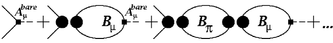
Figure 12: The series of dispersion graphs for $<Q\bar{Q}|A_{\mu}(0)|0>$.

$$<Q(k)\bar{Q}(P-k)|A^{aa}_{\mu}(0)|0>=\bar{Q}(P-k)\left[{\gamma_{\mu}\gamma_{5}g_{A}(P^{2})+P_{\mu}\gamma_{5}h_{A}(P^{2})}\right]Q(k)$$ (73)

with

$$g_{A}(P^{2})= g_{A}^{0}(P^{2})$$

$$h_{A}(P^{2})= h^{0}_{A}(P^{2}) -\frac{G(P^{2})}{1-B_{\pi}(P^{2})}4m[g^{0}_{A}(P^{2})-\frac{P^{2}}{2m}h^{0}_{A}(P^{2})]\int\frac{ds\;G(s)}{\pi(s-M^{2})}\frac{1}{16\pi}\sqrt{1-4m^{2}/s}$$

The form factor $h_{A}$ develops a pole at $P^{2}=m^{2}_{\pi}$ as $B_{\pi}(m^{2}_{\pi})=1$. Near $P^{2}=m^{2}_{\pi}$ one has

$$<\bar{Q}Q|A_{\mu}|0>=<\bar{Q}Q|\pi>\frac{1}{m^{2}_{\pi}-P^{2}}<\pi|A_{\mu}|0>.$$ (74)

Comparing the pole terms in (34) and (35) and using the relation

$$<\pi|Q\bar{Q}>=\frac{\bar{Q}i\gamma_{5}Q}{\sqrt{N_{c}}}G_{v}$$

one finds

$$<\pi|A^{aa}_{\mu}(0)|0>=iP_{\mu}4m[g^{0}_{A}(m^{2}_{\pi})-\frac{m^{2}_{\pi}}{2m}h^{0}_{A}(m^{2}_{\pi})]\sqrt{N_{c}}\int\frac{ds\;G_{v}(s)}{\pi(s-M^{2})}\frac{1}{16\pi}\sqrt{1-4m^{2}/s}=iP_{\mu}f_{\pi}$$ (75)

and hence

$${4m\kappa\sqrt{N_{c}}}\int\frac{ds\;G_{v}(s)}{\pi(s-M^{2})}\frac{1}{16\pi}\sqrt{1-4m^{2}/s}={f_{\pi}}$$ (76)

with

$$\kappa=g_{A}^{0}(m^{2}_{\pi})-\frac{m^{2}_{\pi}}{2m}h_{A}^{0}(m^{2}_{\pi})$$ (77)

We can neglect the second term because the small value $h_{A}^{0}$ is further suppressed by $m^{2}_{\pi}$. Finally, one finds

$$\kappa\approx g_{A}^{0}(m^{2}_{\pi})\approx g_{A}^{0}(0)\approx 0.75\div 1$$ (78)

In terms of the light-cone wave function (76) takes the form

$$\kappa\frac{\sqrt{N_{c}}}{\sqrt{2}\pi}\int{dx\;dk^{2}_{\perp}}\frac{m}{\sqrt{m^{2}+k^{2}_{\perp}}}\;\psi(x,k_{\perp})={f_{\pi}}$$ (79)

7 Appendix C: Soft–hard form factor

The soft–hard form factor $F^{sh}$, given by the graph of Fig.13,

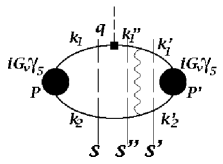
Figure 13: The soft–hard contribution $F^{sh}_{\pi}$ to pion form factor.

accounts for the assumption that at $s^{\prime\prime}>s_{0}$ the $\bar{Q}Q$ interaction is described by the convolution of the one–gluon exchange kernel with the soft–region vertex $G_{v}$ (the right block in Fig.13). To derive the spectral density of $F^{sh}$, we start with the corresponding Feynman graph with pointlike vertices

$$2P_{\mu}(q)\;F^{sh}(q^{2})=\frac{Sp(\lambda^{A}\lambda^{A})}{4N_{c}}g^{2}\int\frac{dk}{(2\pi)^{4}i}\frac{dk^{\prime}}{(2\pi)^{4}i}$$ (80)

$$\times\frac{1}{m^{2}-k^{2}}\frac{1}{m^{2}-(P-k)^{2}}\frac{1}{m^{2}-(P^{\prime}-k)^{2}}\frac{1}{m^{2}-k^{\prime 2}}\frac{1}{m^{2}-(P^{\prime}-k^{\prime})^{2}}\frac{1}{\mu^{2}-(k^{\prime}-k)^{2}}$$

$$\times Sp\left({(\hat{k}_{1}+\hat{q}+m)\gamma_{\mu}(\hat{k}_{1}+m)i\gamma_{5}(m-\hat{k}_{2})\gamma_{\alpha}(m-\hat{k}^{\prime}_{2})i\gamma_{5}(\hat{k}^{\prime}_{1}+m)\gamma^{\alpha}}\right)$$

To allow only for two–particle intermediate states we consider the contribution of $s$, $s^{\prime\prime}$, and $s^{\prime}$ cuts and neglect the contribution of three–particle intermediate states with cutting the gluon line: three–particle states are beyond the scope of our consideration. The resulting spectral density over both soft $s$ and $s^{\prime}$ reads

$$\Delta^{sh}(s^{\prime},s,q^{2})=\theta(s<s_{0})\theta(s^{\prime}<s_{0})\;g^{2}\;C_{F}\int\frac{ds^{\prime\prime}}{s^{\prime\prime}-m^{2}_{\pi}}\theta(s^{\prime\prime}>s_{0})\;Tr(s,s^{\prime},s^{\prime\prime},q^{2})$$ (81)

$$\times\int\frac{dk_{1}dk_{2}dk^{\prime\prime}_{1}}{8\pi^{2}}\delta(k^{2}_{1}-m^{2})\delta(k^{2}_{2}-m^{2})\delta(k^{\prime\prime 2}_{1}-m^{2})\delta(P-k_{1}-k_{2})\delta(P^{\prime\prime}-k_{1}^{\prime\prime}-k_{2})\delta(k^{\prime\prime}_{1}-k_{1}-q)$$

$$\times\int\frac{dk^{\prime}_{1}dk^{\prime}_{2}}{8\pi^{2}}\delta(k^{\prime 2}_{1}-m^{2})\delta(k^{\prime 2}_{2}-m^{2})\delta(P^{\prime}-k_{1}^{\prime}-k^{\prime}_{2})\frac{1}{m_{G}^{2}-(k_{2}-k^{\prime}_{2})^{2}}$$

with $P^{2}=s,\;P^{\prime\prime 2}=s^{\prime\prime},\;P^{\prime 2}=s^{\prime}$.

The quantity $Tr(s,s^{\prime},s^{\prime\prime},q^{2})$ is the dispersion expression for the fermion–loop trace with all fermions taken on mass shell (for details see the Appendix D)

$$Sp\left({(\hat{k}_{1}+\hat{q}+m)\gamma_{\mu}(\hat{k}_{1}+m)i\gamma_{5}(m-\hat{k}_{2})\gamma_{\alpha}(m-\hat{k}^{\prime}_{2})i\gamma_{5}(\hat{k}^{\prime}_{1}+m)\gamma^{\alpha}}\right)=2P_{\mu}(q)Tr$$ (82)

$$Tr=2s^{\prime}\left({\alpha(s^{\prime\prime},s,q^{2})(s^{\prime\prime}+s-q^{2})+q^{2}}\right)-4m^{2}\left({\alpha(s^{\prime\prime},s,q^{2})(s^{\prime}+s-q^{2})+q^{2})}\right)$$

where

$$\alpha(s^{\prime\prime},s,q^{2})=\frac{-q^{2}(s^{\prime\prime}+s-q^{2})}{(s^{\prime\prime}-s)^{2}-2q^{2}(s^{\prime\prime}+s)+q^{4}}$$

Use again the light–cone variables (18). Performing $k_{-}$ integration and denoting $k=k_{2}$, $k^{\prime}=k^{\prime}_{2}$, $x=k_{2+}/P_{+}$, $x^{\prime}=k^{\prime}_{2+}/P_{+}$, $k_{\perp}=k_{2\perp}$, $k^{\prime}_{\perp}=k^{\prime}_{2\perp}$ we come to the final expression

$$F^{sh}(q_{\perp}^{2})=4\pi C_{F}\int\frac{dxd^{2}k_{\perp}}{16\pi^{3}x(1-x)^{2}}\frac{G_{v}(s)\theta(s<s_{0})}{\frac{m^{2}+k^{2}_{\perp}}{x(1-x)}-m^{2}_{\pi}}\frac{\theta(s^{\prime\prime}>s_{0})}{\frac{m^{2}+(k_{\perp}-xq_{\perp})^{2}}{x(1-x)}-m^{2}_{\pi}}$$ (83)

$$\times\frac{dx^{\prime}d^{2}k^{\prime}_{\perp}}{16\pi^{3}x^{\prime}(1-x^{\prime})}\frac{G_{v}(s^{\prime})\theta(s^{\prime}<s_{0})}{\frac{m^{2}+(k^{\prime}_{\perp}-x^{\prime}q_{\perp})^{2}}{x^{\prime}(1-x^{\prime})}-m^{2}_{\pi}}Tr(s,s^{\prime},s^{\prime\prime},q^{2})\frac{\alpha_{s}\left({-(k-k^{\prime})^{2}}\right)}{m_{G}^{2}-(k^{\prime}-k)^{2}}$$

where

$$-(k^{\prime}-k)^{2}=\frac{(k^{\prime}_{\perp}x-k_{\perp}x^{\prime})^{2}+m^{2}(x-x^{\prime})^{2}}{xx^{\prime}}$$

and

$$s=\frac{m^{2}+k_{\perp}^{2}}{x(1-x)},\quad s^{\prime\prime}=\frac{m^{2}+(k_{\perp}-xq_{\perp})^{2}}{x(1-x)},\quad s^{\prime}=\frac{m^{2}+(k^{\prime}_{\perp}-x^{\prime}q_{\perp})^{2}}{x^{\prime}(1-x^{\prime})}$$

In (83) the renormalization $g^{2}\to 4\pi\alpha_{s}(-(k-k^{\prime})^{2})$ is taken into account.

The distribution amplitude which describes the large-$Q^{2}$ behavior of the form factor (see 31) is expressed through $G_{v}$ as

$$\phi(x,s_{0})=4m\sqrt{N_{c}}{\kappa}\int\frac{ds\;G_{v}(s)}{16\pi^{2}(s-m^{2}_{\pi})}\theta\left({\frac{m^{2}}{x(1-x)}<s}\right)\theta(s<s_{0})$$ (84)

8 Appendix D: Trace calculation in the soft–hard contribution

The soft–hard contribution is described by two-loop graph, and the dispersion technique prescribes that the total momenta squared of the $\bar{Q}Q$ pair should be taken different for each loop, and then the integration over these values should be performed. So, we must first make the Fierz rearrangements to obtain trace calculations related to different loops. Namely, we group the expressions as follows

$$2P_{\mu}(q)Tr\equiv Sp\left({(\hat{k}^{\prime\prime}_{1}+m)\gamma_{\mu}(\hat{k}_{1}+m)i\gamma_{5}(m-\hat{k}_{2})\gamma_{\alpha}(m-\hat{k}^{\prime}_{2})i\gamma_{5}(\hat{k}^{\prime}_{1}+m)\gamma^{\alpha}}\right)$$

$$=Sp\left[{(\hat{k}^{\prime\prime}_{1}+m)\gamma_{\mu}(\hat{k}_{1}+m)i\gamma_{5}(m-\hat{k}_{2})}\right]\gamma_{\alpha}\left[{(m-\hat{k}^{\prime}_{2})i\gamma_{5}(\hat{k}^{\prime}_{1}+m)}\right]\gamma^{\alpha}$$

$$=\sum\limits_{i=S,V,T,A,P}\quad C_{i}\times Sp\left[{(\hat{k}^{\prime\prime}_{1}+m)\gamma_{\mu}(\hat{k}_{1}+m)i\gamma_{5}(m-\hat{k}_{2})O_{i}}\right]Sp\left[{(m-\hat{k}^{\prime}_{2})i\gamma_{5}(\hat{k}^{\prime}_{1}+m)O_{i}}\right]$$

with $C_{S}=1,C_{V}=-\frac{1}{2},C_{A}=\frac{1}{2},C_{P}=-1$. The second trace is nonzero only for $A$ and $P$ and we find

$$2P_{\mu}(q)Tr=\frac{1}{2}Sp\left[{(\hat{k}_{1}+\hat{q}+m)\gamma_{\mu}(\hat{k}_{1}+m)i\gamma_{5}(m-\hat{k}_{2})\gamma_{5}\gamma_{\alpha}}\right]Sp\left[{(m-\hat{k}^{\prime}_{2})i\gamma_{5}(\hat{k}^{\prime}_{1}+m)\gamma_{\alpha}\gamma_{5}}\right]$$

$$-Sp\left[{(\hat{k}_{1}+\hat{q}+m)\gamma_{\mu}(\hat{k}_{1}+m)i\gamma_{5}(m-\hat{k}_{2})\gamma_{5}}\right]Sp\left[{(m-\hat{k}^{\prime}_{2})i\gamma_{5}(\hat{k}^{\prime}_{1}+m)\gamma_{5}}\right]\equiv 2P_{\mu}(q)(Tr_{A}+Tr_{P})$$

Each of the expressions $Tr_{i}$ ($i=A,P$) is represented as a product of two factors, related to two different loops (see Fig.14)

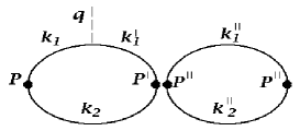
Figure 14: Two loops in $F^{sh}$: momentum notation.

We must use the following relations

$$k_{1}+k_{2}=P,P^{2}=s,\quad k^{\prime\prime}_{1}=k_{1}+q,k^{\prime\prime}_{1}+k_{2}=P^{\prime\prime},P^{\prime\prime 2}=s^{\prime\prime}$$

for the left loop and

$$k^{\prime}_{1}+k^{\prime}_{2}=P^{\prime},P^{\prime 2}=s^{\prime}$$

for the right one and set $all$ the fermions on mass shell. This procedure yields

$$Tr_{A}=-4m^{2}[\alpha(s^{\prime\prime},s,q^{2})(s^{\prime}+s-q^{2})+q^{2}]$$

$$Tr_{P}=2s^{\prime}[\alpha(s^{\prime\prime},s,q^{2})(s^{\prime\prime}+s-q^{2})+q^{2}]$$

And the final result reads

$$Tr=\left[{2s^{\prime}\left({\alpha(s^{\prime\prime},s,q^{2})(s^{\prime\prime}+s-q^{2})+q^{2}}\right)-4m^{2}\left({\alpha(s^{\prime\prime},s,q^{2})(s^{\prime}+s-q^{2})+q^{2})}\right)}\right]$$

References

-
[1]
S.J.Brodsky and G.P.Lepage, Phys.Lett. B87, 359 (1979),
Phys.Rev. D22, 2157 (1980);
A.V.Efremov and A.V.Radyushkin A.V., JETF Lett. 25, 210 (1977), Phys.Lett. B94, 45 (1980);
V.L.Chernyak and A.R.Zhitnitsky, Yad.Fiz. 31, 1053 (1980). - [2] S.J.Brodsky and G.P.Lepage, Exclusive Processes in QCD, in Perturbative QCD, World Scientific, Singapore, 1989, pp.93-241.
- [3] V.L.Chernyak and A.R.Zhitnitsky, Phys.Rep.112, 173 (1984).
- [4] N.Isgur and C.Llewellin-Smith, Phys.Lett. B217, 535 (1989), Nucl.Phys. B317, 526 (1989).
- [5] S.Mikhailov and A.Radyushkin, Phys.Rev. D45, 1754 (1991).
- [6] V.Braun and I.Halperin, Phys.Lett. B328, 457 (1994).
- [7] H.-N.Li and G.Sterman, Nucl.Phys. B382, 129 (1992).
- [8] A.Radyushkin, Qualitative and quantitative aspects of the QCD theory of elastic form factors, CEBAF-TH-93-12 (1993); Pion wave function from QCD sum rules with nonlocal condensates, CEBAF-TH-94-13 (hep-ph/9406237) 1994.
- [9] T.Huang and Q.-X.Shen, Z.Phys. C50, 139 (1991); T.Huang, B.-Q.Ma and Q.-X.Shen, Phys.Rev. D49, 1490 (1993).
- [10] H.Fritzsch, Mod.Phys.Lett. A5, 625 (1990), CERN-TH. 7079/1993.
- [11] S.Weinberg, Phys.Rev.Lett. 65, 1181 (1991); ibid. 67, 3473 (1991).
- [12] N.Isgur and G.Karl, Phys.Lett. B72, 109 (1977).
- [13] Z.Dziembowski, Phys.Rev. D37, 778 (1988).
- [14] W.Jaus, Phys.Rev. D44, 2319 (1991).
- [15] F.Schlumpf,Phys.Rev. D47, 4114 (1993); SLAC-PUB-6483, hep-ph 9406267 (1994).
- [16] F.Cardarelli, I.Grach, I.Narodetskii, E.Pace, G.Salme, and S.Simula, Preprint INFN–ISS 94/3 (1994).
- [17] M.V.Terent’ev, Sov.J.Nucl.Phys. 24, 106 (1976); V.B.Berestetskii and M.V.Terent’ev, Sov. J. Nucl. Phys. 24, 106 (1976), 25, 347 (1977).
- [18] V.V.Anisovich, D.I.Melikhov, B.C.Metsch, and H.R.Petry, Nucl.Phys. A563, 549 (1993).
-
[19]
G. Parisi and R.Petronzio, Phys. Lett., B94,
51 (1980);
M.Consoli and J.H.Field, Phys.Rev.,49, 1293 (1994). -
[20]
C.Bebek et al., Phys.Rev. D13, 25 (1976),
Phys.Rev. D17, 1693 (1978);
S.R.Amendolia et al., Nucl.Phys. B277, 168 (1986). - [21] J.Badier et al., Z.Phys. C – Particles and Fields 18, 281 (1983).
- [22] L.N.Lipatov, Sov.Phys.JETP, 63, 904 (1986).
- [23] V.V.Anisovich, M.N.Kobrinsky, D.I.Melikhov, and A.V.Sarantsev, Nucl.Phys. A544, 747 (1992).