PRECISE PREDICTIONS FOR MASSES AND COUPLINGS

IN THE MINIMAL SUPERSYMMETRIC STANDARD MODEL

J. BAGGER, K. MATCHEV AND D. PIERCE

Department of Physics and Astronomy

The Johns Hopkins University

Baltimore, MD  21218,  USA

We present selected results of our program to determine the masses, gauge couplings, and Yukawa couplings of the minimal supersymmetric model in a full one-loop calculation. We focus on the precise prediction of the strong coupling $\alpha_{s}(M_{Z})$ in the context of supersymmetric unification. We discuss the importance of including the finite corrections and demonstrate that the leading-logarithmic approximation can significantly underestimate $\alpha_{s}(M_{Z})$ when some superpartner masses are light. We show that if GUT thresholds are ignored, and the superpartner masses are less than about 500 GeV, the prediction for $\alpha_{s}(M_{Z})$ is quite large. We impose constraints from nucleon decay experiments and find that minimal SU(5) GUT threshold corrections increase $\alpha_{s}(M_{Z})$ over most of the parameter space. We also consider the missing-doublet SU(5) model and find that it predicts preferred values for the strong coupling, even for a very light superpartner spectrum. We briefly discuss predictions for the bottom-quark mass in the small $\tan\beta$ region.

1 Introduction

The exact one-loop corrections to the masses, gauge couplings and Yukawa couplings of the minimal supersymmetric model are described in Ref. [1]. These corrections are essential ingredients for accurate tests of grand unification. They allow one to extract the underlying $\overline{\it DR}$ parameters from a given set of measured observables. The $\overline{\it DR}$ parameters can then be run up to a high scale to explore the consequences of different unification hypotheses.

Alternatively, the radiative corrections can be used to translate various limits into excluded regions of the $\overline{\it DR}$ parameter space. This is illustrated in Fig. 1, where we show the excluded region of the $M_{0},\ M_{1/2}$ parameter space at the tree and one-loop levels, from current experimental constraints. Here, “tree-level” means that the superpartner masses are determined from the $\overline{\it DR}$ parameters evaluated at the scale $M_{Z}$. For the Higgs mass, the tree-level curve corresponds to the one-loop mass neglecting the gauge/Higgs/gaugino/Higgsino contributions.

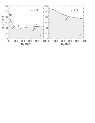
Figure 1: Excluded region (shaded) of the $M_{0},\ M_{1/2}$ plane, for $\tan\beta=2,\ m_{t}=170$ GeV, and $A_{0}=0$. All masses are evaluated at one-loop. The symbols indicate which experimental constraint is relevant: $\chi^{+}\Rightarrow m_{\chi^{+}}>47$ GeV; $\tilde{g}\Rightarrow m_{\tilde{g}}>125$ GeV; $\tilde{\nu}\Rightarrow m_{\tilde{\nu}}>42$ GeV; $h\Rightarrow m_{h}>58$ GeV; $\chi^{0}\Rightarrow$ direct searches for neutralinos at LEP. The dashed line shows the boundary of the excluded region at tree-level.

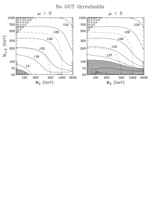
Figure 2: Contours of $\alpha_{s}(M_{Z})$ in the $M_{0}$, $M_{1/2}$ plane, with $\tan\beta=2$, $m_{t}=170$ GeV, and $A_{0}=0$. The contours of squark mass 500 and 1000 GeV are shown by dot-dashed lines. The $\times$’s in the upper left hand corners indicate regions in which the tau sneutrino is the LSP. The shaded regions are excluded by particle searches.

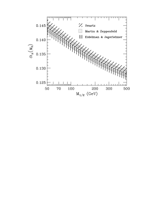
Figure 3: Predictions for $\alpha_{s}(M_{Z})$ using three different values for the QED coupling $\alpha(M_{Z})$. In each case we show the $\pm 1$–$\sigma$ bands, for $\tan\beta=2,\ m_{t}=170$ GeV, $A_{0}=0$, and $\mu>0$.

Figure 4: Comparison of $\alpha_{s}(M_{Z})$ in the leading logarithm approximation (LLA) versus the full one-loop calculation, for $\tan\beta=2,\ m_{t}=170$ GeV, $A_{0}=0$, and $\mu>0$. The dashed line shows the result if the non-universal corrections are neglected.

Figure 5: The smallest triplet Higgs mass allowed by nucleon decay constraints in minimal SU(5), with $\tan\beta=2,\ m_{t}=$170 GeV, $A_{0}=0$, and $\mu>0$. The GUT scale is also shown.

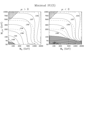
Figure 6: Contours of the smallest possible $\alpha_{s}(M_{Z})$ consistent with nucleon decay in minimal SU(5), with $\tan\beta=2,\ m_{t}=170$ GeV, and $A_{0}=0$. The dot-dashed lines indicate contours of 500 and 1000 GeV squark masses. The $\times$’s indicate the region where the LSP is charged, and the lower shaded regions are excluded by particle searches.

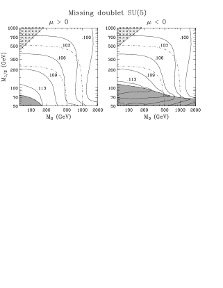
Figure 7: Contours of the minimum possible $\alpha_{s}(M_{Z})$ consistent with nucleon decay in the missing-doublet model, with $\tan\beta=2,\ m_{t}$=170 GeV, and $A_{0}=0$. The shading and dashed lines are as in Fig. 6.

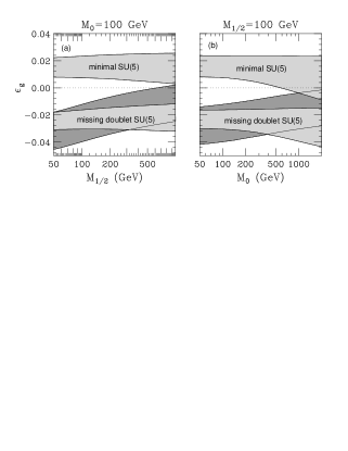
Figure 8: The light shaded regions indicate the allowed values of the gauge coupling threshold correction $\varepsilon_{g}$ in the minimal and missing-doublet SU(5) models. The dark shaded region indicates the range of $\varepsilon_{g}$ necessary to obtain $\alpha_{s}(M_{Z})=0.117\pm 0.01$. For $\tan\beta=2,\ m_{t}=170$ GeV, $A_{0}=0$, and $\mu>0$. (From Ref. [15].)

Figure 9: The bottom-quark mass and $\alpha_{s}(M_{Z})$ vs. $m_{t}$ for the case of no GUT-scale thresholds, for various values of $\tan\beta$, with $A_{0}=0$, $\mu>0$, and $\hat{\lambda}_{t}(M_{\rm GUT})=3$. The right (solid) leg in each pair of lines corresponds to $M_{1/2}$ varying from 60 to 1000 GeV, with $M_{0}$ fixed at 60 GeV. The left (dashed) leg corresponds to $M_{0}$ varying from 60 to 1000 GeV, with $M_{1/2}=100$ GeV. On the solid lines the circles mark, from top to bottom, $M_{1/2}=60$, 100, 200, 400, and 1000 GeV, and on the dashed lines the circles mark $M_{0}=60$, 200, 400, and 1000 GeV. Note that the lowest point on each left leg and the second-to-lowest point on each right leg corresponds to $m_{\tilde{q}}\simeq 1$ TeV. The horizontal dashed lines indicate $m_{b}=5.2$ GeV and $\alpha_{s}(M_{Z})=0.127$. The $\times$’s mark points with one-loop Higgs mass $m_{h}<60$ GeV. (From Ref. [15].)

Figure 10: The bottom-quark mass vs. the top-quark mass for fixed values of $\alpha_{s}(M_{Z})$ and various $\tan\beta$. The solid lines correspond to $\hat{\lambda}_{t}(M_{\rm GUT})=3$ while the dashed lines correspond to $\hat{\lambda}_{t}(M_{\rm GUT})=2$. The upper line in each pair corresponds to a light supersymmetric spectrum with $M_{0}=M_{1/2}=80$ GeV. The lower line in each pair corresponds to a heavy spectrum, $M_{0}=1000$ GeV, $M_{1/2}=500$ GeV. The dotted lines delineate the preferred region $4.7<m_{b}<5.2$ GeV. For $A_{0}=0$ and $\mu>0$.

The study of gauge coupling unification has been carried out by many groups beginning more than 20 years ago. There has been a resurgence during the last five years. The analyses have become increasingly more refined. The most recent analyses use the full set of two-loop RGE’s to predict the strong coupling constant as a function of the electroweak input parameters. They pay proper attention to $\overline{\it MS}$ - $\overline{\it DR}$ differences and treat the weak thresholds in different levels of detail.

Over time, the predicted value of the strong coupling constant has increased markedly, in part due to the refinements mentioned above, but more so from the fact that the standard-model weak mixing angle, as determined by a global fit to the data, has been steadily decreasing. (This is correlated with the increasing best-fit value for the top-quark mass.)

In this talk we take a closer look at supersymmetric unification. We treat the supersymmetric threshold corrections in a complete one-loop analysis. Our work stands in contrast to most previous studies, which are based on the “leading logarithm approximation.” This approximation involves taking the standard-model value of $\sin^{2}\theta_{W}$ and adding the logarithmic parts of the SUSY threshold corrections. The approximation works well if all of the SUSY particle masses are much greater than $M_{Z}$, in which case the decoupling theorem implies that the finite effects of the SUSY particles are negligible for all low-energy observables.

However, in realistic models it is not unusual for the supersymmetric spectrum to contain light particles of order the $Z$-mass. In this case one cannot use the standard-model value of $\sin^{2}\theta_{W}$ as an input into a precision analysis. This is because the quoted value of $\sin^{2}\theta_{W}$ is the result of a fit to the data, assuming that the standard model is correct. The experimental analyses do not include the finite SUSY corrections, which are different for each observable. Therefore in our analysis, we use a single set of inputs in our calculation of $\sin^{2}\theta_{W}$, namely, $\alpha_{EM}$, $G_{F}$, $M_{Z}$, $m_{t}$, and the parameters that describe the supersymmetric model.

We note that a careful evaluation of the weak mixing angle is important for determining a precise prediction for $\alpha_{s}(M_{Z})$. Using the one-loop RGE’s and the condition of coupling unification, we find that the three gauge couplings satisfy

$${\beta_{2}-\beta_{3}\over\hat{g}_{1}^{2}(\mu)}\ +\ {\beta_{3}-\beta_{1}\over\hat{g}_{2}^{2}(\mu)}\ +\ {\beta_{1}-\beta_{2}\over\hat{g}_{3}^{2}(\mu)}\ =\ 0\ ,$$ (1)

where $\beta_{i}$ are the three beta functions, $d\hat{g}_{i}/dt=\beta_{i}\hat{g}_{i}^{3}/16\pi^{2}$. These relations imply that

$${\delta\alpha_{s}\over\alpha_{s}(M_{Z})}\ \simeq\ \,{\delta\hat{\alpha}\over\hat{\alpha}}\ -\ 7.5\ {\delta\hat{s}^{2}\over\hat{s}^{2}}\ .$$ (2)

Hence, an error in the determination of $\hat{s}^{2}$ of 1% leads to an error in $\alpha_{s}(M_{Z})$ of 7.5%.

In this talk we use the full set of one-loop radiative corrections to evaluate the $\overline{\it DR}$ gauge and Yukawa couplings. The $\overline{\it DR}$ couplings serve as the boundary conditions for the two-loop gauge and Yukawa coupling renormalization group equations (RGE’s), which determine the couplings at very high scales. In what follows we use the full one-loop corrections at both the weak and GUT scales to determine the regions of supersymmetric parameter space that permit gauge and Yukawa coupling unification.

2 Calculation of $\hat{s}^{2}$

Given the inputs $\alpha_{EM}=1/137.036$, $G_{F}=1.16639\times 10^{-5}$ GeV^-2, and $M_{Z}=91.187$ GeV, as well as $m_{t}$ and the parameters of the supersymmetric model, we determine [3] ($\hat{c}^{2}=1-\hat{s}^{2}$)

$$\hat{\alpha}={\alpha_{EM}\over(1-\Delta\hat{\alpha})}\qquad\mbox{and}\qquad\hat{c}^{2}\hat{s}^{2}={\pi\,\alpha_{EM}\over\sqrt{2}\,G_{F}\,M_{Z}^{2}\,(1-\Delta\hat{r})}\ .$$

Here $\Delta\hat{\alpha}$ contains logarithms of the masses of the charged particles, and

$$\Delta\hat{r}=\Delta\hat{\alpha}-{\hat{\Pi}_{Z}(M_{Z}^{2})\over M_{Z}^{2}}+{\hat{\Pi}_{W}(0)\over M_{W}^{2}}+\mbox{vertex $+$ box}\ .$$

The vertex and box diagram contributions are the so-called “non-universal” or “non-oblique” corrections, and the remaining corrections involve the real and transverse parts of the $\overline{\it DR}$ gauge boson self-energies. The vertex and box corrections vanish in the leading logarithm approximation; the correction $\Delta\hat{\alpha}$ contains only logarithms; and the $W$ and $Z$ self-energies contain both logarithmic and finite corrections.

In our calculation of $\Delta\hat{r}$ we include the dominant two-loop corrections (given in Ref.  [4]), which leads to a very precise determination of $\hat{s}^{2}$. Following Ref.  [2], we estimate the theoretical uncertainty in $\hat{s}^{2}$ to be about 1 part in 10⁴, while the experimental uncertainty (due to the uncertainty in the determining the electromagnetic coupling at the $Z$-scale) is 2.6 parts in $10^{4}$. Having determined $\hat{\alpha}$ and $\hat{s}^{2}$ precisely, we are in position to fix the boundary conditions for the two-loop RGE’s [5],

$$\hat{\alpha}\equiv{\hat{e}^{2}\over 4\pi},\quad\hat{s}^{2}\qquad\longrightarrow\qquad\hat{g}_{1}=\sqrt{5\over 3}{\hat{e}\over\hat{c}},\quad\hat{g}_{2}={\hat{e}\over\hat{s}}\ ,$$

and accurately investigate gauge coupling unification.

In the following we assume that the SUSY masses unify at the scale $M_{\rm GUT}$ (which is defined as the scale where $\hat{g}_{1}$ and $\hat{g}_{2}$ meet). Therefore the supersymmetric model is parametrized by a universal gaugino mass $M_{1/2}$, a universal scalar mass $M_{0}$, and a universal trilinear scalar coupling $A_{0}$. The ratio of $\overline{\it DR}$ vacuum expectation values evaluated at the scale $M_{Z}$ is denoted $\tan\beta$. We require the parameters to be such that electroweak symmetry is spontaneously broken. These conditions determine the value of $\mu^{2}$, the supersymmetric Higgs mass parameter, and $m_{A}$, the CP-odd neutral Higgs boson mass, once we specify the sign of $\mu$.

3 Prediction for $\alpha_{s}(M_{Z})$

As a reference point, we show in Fig. 2 contours of $\alpha_{s}(M_{Z})$ in the $M_{0},\ M_{1/2}$ plane, with no GUT thresholds, $\tan\beta=2$, $m_{t}=170$ GeV, and $A_{0}$=0. We find $\alpha_{s}(M_{Z})$ is large compared to the PDG value [6] $\alpha_{s}(M_{Z})=0.117\pm 0.005$, especially near $M_{0},\ M_{1/2}=100$ GeV.

The experimental uncertainty in the determination of $\alpha_{s}(M_{Z})$ is primarily due to the uncertainty in determining the electromagnetic coupling at the $Z$-scale. We use the value recently determined by Eidelman and Jegerlehner [7]. Martin and Zeppenfeld [8] and Swartz [9] have also performed analyses to determine $\alpha(M_{Z})$. We show in Fig. 3 the differences in the determination of $\alpha_{s}(M_{Z})$ using the various values of $\alpha(M_{Z})$.

As stated in the introduction, the finite corrections can be significant when some of the superpartners have masses of order $M_{Z}$. This is illustrated in Fig. 4, where we compare the value of $\alpha_{s}(M_{Z})$ in the leading logarithm approximation (LLA) with the value obtained in the full calculation. In Fig. 4(a) the full and LLA curves converge for large $M_{1/2}$ because the SUSY particles decouple. In Fig. 4(b) the full and LLA curves do not converge as $M_{0}$ becomes large. This is because $M_{1/2}=60$ GeV, so the gauginos remain light for arbitrarily large $M_{0}$.

To summarize our results for $\alpha_{s}(M_{Z})$ in the absence of GUT threshold corrections, we find $\alpha_{s}(M_{Z})>0.126$ for squark masses less than 1 TeV, with $m_{t}=170$ GeV. For a SUSY spectrum of 500 GeV or less, we have $\alpha_{s}(M_{Z})>0.130$.

If we require smaller values of $\alpha_{s}(M_{Z})$ and a light supersymmetric spectrum, a GUT threshold correction is clearly needed. We can parametrize the GUT threshold correction by $\varepsilon_{g}$, where

$$\hat{g}_{3}(M_{\rm GUT})=\hat{g}_{\rm GUT}(M_{\rm GUT})\left(1+\varepsilon_{g}\right)\ ,$$

and $\hat{g}_{\rm GUT}\equiv\hat{g}_{1}(M_{\rm GUT})=\hat{g}_{2}(M_{\rm GUT})$. A smaller value of $\alpha_{s}(M_{Z})$ requires $\varepsilon_{g}<0$. In what follows we examine the value of $\varepsilon_{g}$ in two SU(5) GUT models.

In the minimal SU(5) model [10], the gauge coupling threshold correction $\varepsilon_{g}^{\prime}$ is given by [11]

$$\varepsilon^{\prime}_{g}\ =\ {3g_{\rm GUT}^{2}\over 40\pi^{2}}\,\log\left(M_{H_{3}}\over M_{\rm GUT}\right)\ ,$$ (3)

where $M_{H_{3}}$ is the mass of the color-triplet Higgs particle that mediates nucleon decay. From this expression, we see that $\varepsilon^{\prime}_{g}<0$ whenever $M_{H_{3}}<M_{\rm GUT}$. However, $M_{H_{3}}$ is bounded from below by proton decay experiments. The $M_{H_{3}}$ mass limit is of the form [12]

$$M_{H_{3}}>{\cal M}\ {|1+y^{tK}|\over\sin 2\beta}f(\tilde{w},\tilde{d},\tilde{u},\tilde{e})$$

where ${\cal M}$ is a nuclear matrix element, $y^{tK}$ parametrizes the amount of third generation mixing, and $f$ is a function of the wino, squark and slepton masses.

In Fig. 5 we show the minimum value for $M_{H_{3}}$ from the nucleon decay constraint, for the conservative choices ${\cal M}=0.003$ GeV³ and $|1+y^{tK}|=0.4$. We see that $M_{H_{3}}^{\rm min}>M_{\rm GUT}$ unless $M_{0}>500$ GeV and $M_{1/2}\ll M_{0}$. Thus, in most of the parameter space, $\varepsilon_{g}^{\prime}>0$.

In minimal SU(5), $\alpha_{s}(M_{Z})$ is typically even larger than it was without any GUT thresholds, as illustrated in Fig. 6. The only exception occurs in the region $M_{0}\gg M_{1/2}$, where the proton decay amplitude is suppressed. In this region, with 1 TeV squark masses and $m_{t}=170$ GeV, we find $\alpha_{s}(M_{Z})$ as small as 0.123. In fact, as long as $m_{\tilde{q}}\leq 1$ TeV, $\alpha_{s}(M_{Z})<0.126$ can only be obtained in the region $M_{0}\simeq 1$ TeV. For example, if $M_{0}\leq 500$ GeV, $\alpha_{s}(M_{Z})\geq 0.127$.

The missing-doublet model is an alternative SU(5) theory in which the heavy color-triplet Higgs particles are split naturally from the light Higgs doublets [13]. In this model the GUT gauge threshold correction is given by [14]

$$\varepsilon_{g}^{\prime\prime}\ =\ {3g_{\rm GUT}^{2}\over 40\pi^{2}}\,\Biggl{\{}\log\left(M_{H_{3}}^{\rm eff}\over M_{\rm GUT}\right)-{25\over 2}\log 5+15\log 2\Biggr{\}}\ \simeq\ \varepsilon^{\prime}_{g}-4\%\ .$$ (4)

Thus, for fixed $M_{H_{3}}$, the missing-doublet model has the same threshold correction as the minimal SU(5) model, minus 4%. In eq. (4), $M_{H_{3}}^{\rm eff}$ is the effective mass that enters into the proton decay amplitude, so the bounds on $M_{H_{3}}$ in the minimal SU(5) model also apply to $M_{H_{3}}^{\rm eff}$ in the missing-doublet model.

The large negative correction in eq. (4) is due to the mass splitting in the 75 representation, and gives rise to much smaller values for $\alpha_{s}(M_{Z})$. This is illustrated in Fig. 7, where we show contours of $\alpha_{s}(M_{Z})$ in the $M_{0},\ M_{1/2}$ plane, with $M_{H_{3}}^{\rm eff}=M_{H_{3}}^{\rm min}$. The values of $\alpha_{s}(M_{Z})$ are somewhat low, but one can easily obtain larger values, for example, by increasing $M_{H_{3}}^{\rm eff}$.

In Fig. 8 we illustrate the full range of $\alpha_{s}(M_{Z})$ values in the minimal SU(5) and missing-doublet models. We show the allowed range of $\varepsilon_{g}$ in the two models (setting $M_{H_{3}}^{\rm max}=10^{19}$ GeV), together with the range of $\varepsilon_{g}$ which yields $\alpha_{s}(M_{Z})=0.117\pm 0.01$. The missing doublet model is mostly contained within the preferred region of $\alpha_{s}(M_{Z})$, while minimal SU(5) is almost entirely outside.

4 Yukawa unification

In the final part of this talk, we investigate the possibility of bottom-tau Yukawa coupling unification. Our procedure is as follows. We start with the experimental value for the $\tau$ pole mass $m_{\tau}=1.777$ GeV [6]. We convert it to the $\overline{\it DR}$ running mass and evolve it up to the $Z$-scale, where we apply the SUSY threshold corrections. We compute the $\overline{\it DR}$ vev from the $Z$-boson mass, $\hat{v}^{2}=4(M_{Z}^{2}+\hat{\Pi}_{Z}(M_{Z}^{2}))/(\hat{g}^{\prime 2}+\hat{g}^{2})$, and use it to determine the $\overline{\it DR}$ tau Yukawa coupling

$$\widehat{\lambda}_{\tau}={\sqrt{2}\hat{m}_{\tau}\over\hat{v}\cos\beta}\ .$$

We then solve the RGE’s to find $\widehat{\lambda}_{\tau}(M_{\rm GUT})$, and set the bottom Yukawa coupling to

$$\hat{\lambda}_{b}(M_{\rm GUT})=\widehat{\lambda}_{\tau}(M_{\rm GUT})\left(1+\varepsilon_{b}\right)\ ,$$

where $\varepsilon_{b}$ parametrizes the GUT threshold correction. Once we have $\hat{\lambda}_{b}(M_{\rm GUT})$ we run everything back to the weak scale and self-consistently determine the pole mass for the bottom quark.

Let us first examine the prediction for the bottom-quark pole mass with $\varepsilon_{b}=0$. Generally, the large value of the strong coupling increases the bottom mass so much that the prediction typically falls outside the region determined by experiment [6], which we take to be 4.7 GeV $<m_{b}<5.2$ GeV. Because Yukawa couplings enter the Yukawa RGE’s with the opposite sign from gauge couplings, large Yukawa couplings help reduce the large $b$ mass. In particular, in the very small $\tan\beta$ region, the top Yukawa coupling becomes large. In this infrared fixed point region the bottom mass can be less than 5.2 GeV.

We show in Fig. 9 the prediction for $m_{b}$ and $\alpha_{s}(M_{Z})$, obtained by setting the top Yukawa coupling to be $\widehat{\lambda}_{t}(M_{\rm GUT})=3$. We see that even with this large top Yukawa coupling, which is on the verge of being non-perturbative, $m_{b}$ is larger than 5.2 GeV unless $M_{0}$ or $M_{1/2}$ is greater than about 1 TeV. One needs a GUT threshold correction to reduce $m_{b}$ with a SUSY mass scale below 1 TeV.

The similarity between the curves for $\alpha_{s}(M_{Z})$ and $m_{b}$ in Fig. 9 illustrates the strong correlation between $\alpha_{s}(M_{Z})$ and $m_{b}$. In fact, $m_{b}$ is far more sensitive to the gauge-coupling GUT threshold correction than that of the bottom-quark Yukawa coupling. Numerically, we find

$${\delta m_{b}\over m_{b}}\ \simeq\ 0.8\,\varepsilon_{b}\ +\ 8\,\varepsilon_{g}\ .$$

Hence, if we consider a GUT model where $\varepsilon_{g}$ is sufficiently negative, the central value of $m_{b}$ can be obtained with $\varepsilon_{b}=0$. This is shown in Fig. 10, where, for fixed $\varepsilon_{b}=0$, we show the predicted value of $m_{b}$, assuming various values of $\varepsilon_{g}$ that yield particular values of $\alpha_{s}(M_{Z})$. We show the results for $\widehat{\lambda}_{t}(M_{\rm GUT})=2$ and 3, and for a small and large supersymmetric mass scale. The figure shows that as long as $\varepsilon_{g}$ is such that $\alpha_{s}(M_{Z})\simeq 0.12$, an acceptable value of $m_{b}$ is predicted for $\varepsilon_{b}=0$, independent of the top-quark mass and the supersymmetric mass scale.

5 Conclusion

In this talk we have presented results from a complete calculation of the one-loop corrections to the masses, gauge, and Yukawa couplings in the MSSM. We have seen that such a calculation allows us to reliably investigate various unified models to see whether they are compatible with current experimental data.

In particular, we found that the finite SUSY corrections, which are neglected in the leading logarithm approximation, can substantially increase the prediction for $\alpha_{s}(M_{Z})$ when some of the SUSY partner masses are lighter than or of order $M_{Z}$. In the minimal SU(5) model, we found that $\alpha_{s}(M_{Z})\,\raise 1.29167pt\hbox{$>$\kern-7.5pt\lower 4.30554pt\hbox{$\sim$}}\,0.14$ in the small $M_{SUSY}$ region, $M_{0}\simeq M_{1/2}\simeq 100$ GeV. We also found $\alpha_{s}(M_{Z})>0.123$ in the region where the squark masses are below 1 TeV. In contrast, we showed that the missing-doublet SU(5) model can accommodate much smaller values of $\alpha_{s}(M_{Z})$, such as $\alpha_{s}(M_{Z})\simeq 0.113$ for $M_{0}\simeq M_{1/2}\simeq 100$ GeV.

This work was supported by the U.S. National Science Foundation under grant NSF-PHY-9404057.

References

- [1] J. Bagger, K. Matchev and D. Pierce, to appear.
- [2] P. Chankowski, Z. Płuciennik and S. Pokorski, Warsaw preprint IFT–94/19.
- [3] G. Degrassi, S. Fanchiotti and A. Sirlin, Nucl. Phys. B 351 (1991) 49, and references therein.
- [4] S. Fanchiotti, B. Kniehl and A.Sirlin, Phys. Rev. D 48 (1993) 307.
- [5] M.E. Machacek and M.T. Vaughn, Nucl. Phys. B 222 (1983) 83; ibid. B 236 (1984) 221; ibid. B 249 (1985) 70; I. Jack, Phys. Lett. B 147 (1984) 405; S. Martin, M. Vaughn, Northeastern preprint NUB-3081-93-TH (1993); Y. Yamada Phys. Rev. D 50 (1994) 3537; I. Jack and D.R.T. Jones, Phys. Lett. B 333 (1994) 372.
- [6] Particle Data Group Review of Particle Properties, Phys. Rev. D 50 (1994) 1.
- [7] S. Eidelman and F. Jegerlehner, preprint PSI-PR-95-1, (1995).
- [8] A.D. Martin and D. Zeppenfeld, University of Wisconsin preprint MAD-PH-855 (1994).
- [9] M. Swartz, SLAC preprint SLAC-PUB-6710 (1994).
- [10] S. Dimopoulos and H. Georgi, Nucl. Phys. B 193 (1981) 150; N. Sakai, Z. Phys. C 11 (1981) 153.
- [11] M.B. Einhorn and D.R.T. Jones, Nucl. Phys. B 196 (1982) 475; I. Antoniadis, C. Kounnas and K. Tamvakis, Phys. Lett. B 119 (1982) 377.
- [12] J. Hisano, H. Murayama and T. Yanagida, Nucl. Phys. B 402 (1993) 46.
- [13] A. Masiero, D.V. Nanopoulos, K. Tamvakis and T. Yanagida, Phys. Lett. B 115 (1982) 380; B. Grinstein, Nucl. Phys B 206 (1982) 387.
- [14] K. Hagiwara and Y. Yamada, Phys. Rev. Lett. 70 (1993) 709; see also Y. Yamada, Z. Phys. C 60 (1993) 83.
- [15] J. Bagger, K. Matchev and D. Pierce, Johns Hopkins preprint JHU-TIPAC/95001, hep-ph/9501277, to appear in Phys. Lett. B.