TTP94–32

LBL-36678

hep-ph/9503396

December 1994

QCD Corrections to the $e^{+}e^{-}$ Cross Section and the $Z$ Boson Decay Rate^†
K.G. Chetyrkin ^ab, J.H. Kühn^a, A. Kwiatkowski^c

• Institut für Theoretische Teilchenphysik, Universität Karlsruhe
  D-76128 Karlsruhe, Germany

• Institute for Nuclear Research, Russian Academy of Sciences
  60th October Anniversary Prospect 7a Moscow 117312, Russia

• Theoretical Physics Group, Lawrence Berkeley Laboratory
  University of California, Berkeley, CA. 94720, USA

Abstract

QCD corrections to the electron positron annihilation cross section into hadrons and to the hadronic $Z$ boson decay rate are reviewed. Formal developments are introduced in a form particularly suited for practical applications. These include the operator product expansion, the heavy mass expansion, the decoupling of heavy quarks and matching conditions. Exact results for the quark mass dependence are presented whenever available, and formulae valid in the limit of small bottom mass ($m_{{\rm b}}^{2}\ll s$) or of large top mass ($m_{{\rm t}}^{2}\gg s$) are presented. The differences between vector and axial vector induced rates as well the classification of singlet and nonsinglet rates are discussed. Handy formulae for all contributions are collected and their numerical relevance is investigated. Prescriptions for the separation of the total rate into partial rates are formulated. The applicability of the results in the low energy region, relevant for measurements around 10 GeV and below, is investigated and numerical predictions are collected for this energy region.

emails:
chet@ttpux2.physik.uni-karlsruhe.de
johann.kuehn@physik.uni-karlsruhe.de
kwiat@theor2.lbl.gov

^†To appear in “Reports of the Working Group on Precision Calculations for the Z-resonance” .

The complete postscript file of this preprint, including figures, is available via anonymous ftp at
ttpux2.physik.uni-karlsruhe.de (129.13.102.139) as /ttp94-32/ttp94-32.ps or via www at
http://ttpux2.physik.uni-karlsruhe.de/cgi-bin/preprints/

1 Introduction

Since experiments at the ${\rm e}^{+}{\rm e}^{-}$ storage ring LEP started data-taking a few years ago, and by the end of the 1993 run by the four experiments, more than seven million hadronic events had been collected at the ${Z}$ resonance. The accuracy of the measurements is impressive. Numerous parameters of the standard model can be determined with high precision, allowing stringent tests of the standard model to be performed . Among them: the mass $M_{{Z}}=(91.188\pm 0.0044)$ GeV and the width $\Gamma_{{Z}}=(2.4974\pm 0.0038)$ GeV of the ${Z}$ boson or the weak mixing angle $\sin^{2}\theta_{{\rm eff}}^{{\rm lept}}=0.2322~{}\pm~{}0.0006$ [1]. All experimental results were in remarkable agreement with theoretical predictions and a triumphant confirmation of the standard model.

As well as the electroweak sector of the standard model, LEP provides an ideal laboratory for the investigation of strong interactions. Due to their purely leptonic initial state, events are very clean from both the theoretical and experimental point of view and represent the ideal place for testing QCD. From cross-section measurements $\sigma_{{\rm had}}=(41.49\pm 0.12)$ nbarn [1] as well as from the analysis of event topologies the strong coupling constant can be extracted. Other observables measurable with very high precision are the (partial) ${Z}$ decay rates into hadrons $\Gamma_{{\rm had}}/\Gamma_{{\rm e}}=20.795\pm 0.040$ and bottom quarks $\Gamma_{{\rm b}\overline{{\rm b}}}/\Gamma_{{\rm had}}=0.2192\pm 0.0018$. From the line shape analysis of LEP a value $\alpha_{s}=0.126\pm 0.005\pm 0.002$ is derived. The program of experimentation at LEP is still not complete. The prospect of an additional increase in the number of events by a factor of two to four will further improve the level of accuracy. This means, for example, that the relative uncertainty of the partial decay rate into ${\rm b}$ quarks $\Delta\Gamma_{{\rm b}}/\Gamma_{{\rm b}}$ falls below one percent and that an experimental error for $\alpha_{s}$ of 0.002 may be achieved.

Also at lower energies significant improvements can be expected in the accuracy of cross-section measurements. The energy region of around $10$ GeV just below the ${{\rm B}}{\rm\overline{B}}$ threshold will be covered with high statistics at future B meson factories. The cross section between the charm and bottom thresholds can be measured at the BEPC storage ring in Bejing. These measurements could provide a precise value for $\alpha_{s}$ and — even more important — a beautiful proof of the running of the strong coupling constant.

In view of this experimental situation theoretical predictions for the various observables with comparable or even better accuracy become mandatory and higher-order radiative corrections are required. It seems appropriate to collect all presently available calculations and reliably estimate their theoretical uncertainties. The aim of this report is to provide such a review for the QCD sector of the standard model, as far as cross-section measurements are concerned, at the ${Z}$ peak as well as in the ‘low energy’ region from 5 to 20 GeV. (Related topics have been also discussed in recent reviews [2].) Higher-order QCD corrections to the ${\rm e}^{+}{\rm e}^{-}$ annihilation cross-section into hadrons will be discussed as well as the hadronic width of the ${Z}$ boson. Further interest lies in the partial rates for the decay of the ${Z}$ boson into specific quark channels. Of particular importance is the partial width $\Gamma(Z\rightarrow{\rm b}\overline{{\rm b}})$, as this quantity can be measured with high accuracy and provides important information about the top quark mass from the $Z{\rm b}\overline{{\rm b}}$ vertex. However, the decomposition of $\Gamma_{{\rm had}}$ into partial decay rates of different quark species is possible in a simple, straightforward way only up to corrections of the order of ${\cal O}(\alpha_{s})$. Apart from diagrams where ‘secondary quarks’ are radiated off the ‘primary quarks’ one encounters flavour singlet diagrams that first arise in order ${\cal O}(\alpha_{s}^{2})$ and lead to a confusion of different species. They therefore have to be carefully scrutinized.

For many considerations and experimental conditions quark masses can be neglected, compared to the characteristic energy of the problem. Accordingly, higher-order QCD corrections to the total cross-section were first calculated for massless quarks. At LEP energies this is certainly a good approximation for ${{\rm u,d,s}}$ and ${\rm c}$ quarks. In view of the accuracy reached at LEP much effort has been spent in estimating the size of mass effects of the bottom and the top quark. Whereas ${\rm b}$ quarks are present as particles in the final state, top quarks can appear only through virtual corrections. A large part of this report is devoted to these effects. The application of these formulae and, if necessary, their numerical evaluation will also be covered.

In Part 2 topics of a general nature are addressed. In Section 2.1 the notation is introduced and the relation between cross-sections and decay rates on the one hand and the corresponding current correlators on the other is discussed. Furthermore, the classification of singlet versus nonsinglet terms is introduced. The behaviour of coupling constant, masses, operators and correlators under renormalization group transformations is reviewed in Section 2.2 and the relevant anomalous dimensions are listed. The decoupling of heavy quarks and the resulting matching conditions for coupling constant masses and effective currents are treated in Section 2.3. Numerical values of quark masses are discussed in Section 2.4. Part 3 is concerned with calculational techniques relevant to the problems at hand. Emphasis is put on the behaviour of the current correlators at large momenta, the structure of mass corrections in the small mass limit and the resummation of large logarithms of $m^{2}/s$. And the other extreme, with $s/m^{2}\ll 1$ also dealt with in this Part, which concludes with a discussion of $\gamma_{5}$ in $D\neq 4$ dimensions.

The analytical first-order QCD corrections to the cross-section are recalled in Part 4. Approximations in the limits of low and high energies are given.

Nonsinglet and singlet contributions to the QCD corrections are presented in Parts 5 and 6, respectively, and the relevant formulae for various applications are given. First, the calculations are reviewed for massless quarks. This assumption is evidently not justified for the heavy top top mass, which appears as a virtual particle. Top mass corrections are described in Section 5.2. The dependence on the mass of the final-state quarks is given in Section 5.3. At low energies not only do the leading quadratic mass terms have to be taken into account, but quartic mass terms also become relevant. They are presented in Section 5.4. The influence of secondary quark production on determinations of the partial rate is treated in Section 5.5.

Flavour singlet contributions are discussed in Part 6. They arise for the first time in second order for the axial-induced rate and in third order for the vector current-induced rate. ${\cal O}(\alpha_{s}^{2})$ singlet corrections would be absent for six massless flavours, but do not vanish due to the large mass splitting in the $({\rm b,t})$ doublet. Massless contributions and bottom-mass corrections from singlet diagrams are covered in Sections 6.1 and 6.2 respectively. The assignment of the singlet contributions to a partial rate into a specific quark flavour is explained in Section 6.3. and the resulting ambiguity is discussed. In Part 7 the numerical relevance of the different contributions are studied. Different sources of theoretical uncertainties are investigated and their size estimated.

A collection of formulae is presented in the Appendix. It provides an overview and may serve as a quick and convenient reference for later use.

2 General Considerations

2.1 Notations

2.1.1 Cross-Sections and Decay Rates

We introduce our notations by casting the total cross-section for longitudinally polarized ${\rm e}^{+}{\rm e}^{-}$ into hadrons in leading order of the electroweak coupling as:

$$\sigma_{{{\rm R}\atop{\rm L}}} = \frac{4\pi\alpha^{2}}{3s}\Bigg{\{}\frac{(v_{{\rm e}}\mp a_{{\rm e}})^{2}}{y^{2}}\left|\frac{s}{s-M_{{Z}}^{2}+iM_{{Z}}\Gamma_{{Z}}}\right|^{2}\frac{R^{{\rm V}}+R^{{\rm A}}}{y^{2}}$$ (1)

$$+2Q_{{\rm e}}\frac{v_{{\rm e}}\mp a_{{\rm e}}}{y}{\rm Re}\left[\frac{s}{s-M_{{Z}}^{2}+iM_{{Z}}\Gamma_{{Z}}}\right]\frac{R^{{\rm int}}}{y}+Q_{{\rm e}}^{2}R^{{\rm em}}\Bigg{\}}{}\,,$$

with the weak couplings defined through

$$v_{{f}}=2I_{3}^{{f}}-4Q_{{f}}\sin^{2}\theta_{{\rm w}}\,,\;\;\;\;a_{{f}}=2I_{3}^{{f}}\,,\;\;\;\;y=4\sin\theta_{{\rm w}}\cos\theta_{{\rm w}}{}\,.$$ (2)

$R$ and $L$ denote the electron beam polarization (positrons are assumed to be unpolarized). The functions $R^{{k}}$ with $k={\rm V,A},{\rm em},{\rm int}$ are the natural generalization of the Drell ratio $R\equiv\sigma_{{\rm had}}/\sigma_{\rm point}=R^{{\rm em}}$, which is familiar from purely electromagnetic interactions at lower energies. They are induced by the vector and axial couplings of the ${Z}$ boson, the pure QED part and an interference term. In the massless parton model they are given by

$$R^{{\rm V}}=3\sum_{{f}}v_{{f}}^{2}\,,\;\;\;\;\;R^{{\rm A}}=3\sum_{{f}}a_{{f}}^{2}\,,\;\;\;\;\;R^{{\rm em}}=3\sum_{{f}}Q_{{f}}^{2}\,,\;\;\;\;\;R^{{\rm int}}=3\sum_{{f}}Q_{{f}}v_{{f}}\,.$$ (3)

Here the sum extends over all flavours $f$.

The hadronic decay rate of the ${Z}$ can be expressed in a way similar to the incoherent sum of its vector- and axial vector-induced parts:

$$\begin{array}[]{ll}\displaystyle\Gamma_{{Z}}^{{\rm had}}&\displaystyle=\Gamma^{{\rm V}}+\Gamma^{{\rm A}}\\ &\displaystyle=\frac{\alpha}{3}\frac{M_{{Z}}}{y^{2}}(R^{{\rm V}}+R^{{\rm A}}){}\,.\end{array}$$ (4)

Alternatively one may express $\alpha/y^{2}$ through the Fermi constant

$$\frac{\alpha}{y^{2}}=\frac{G_{{\rm F}}M_{{Z}}^{2}}{8\pi\sqrt{2}}$$ (5)

and absorb the large logarithms from the running of QED. These formulae are equivalent for the present purpose, where higher-order electroweak corrections are ignored.

All relevant information needed for the correction factors $R^{{k}}$ is contained in the current correlation functions

$$\begin{array}[]{rl}\Pi_{\mu\nu}^{ij}(q)=&\displaystyle i\int{\rm d}xe^{iqx}\langle 0|\;T\;j_{\mu}^{{i}}(x)j_{\nu}^{j}(0)\;|0\rangle\\ =&\displaystyle g_{\mu\nu}\Pi_{1}^{ij}(-q^{2})+q_{\mu}q_{\nu}\Pi_{2}^{ij}(-q^{2}){}\,,\end{array}$$ (6)

with $(i,j)={\rm(V,V),(A,A)},({\rm em},{\rm em}),({\rm em,V})$ for $k={\rm V,A},{\rm em},{\rm int}$ respectively. The currents under consideration are defined through

$$j^{{\rm V}}_{\mu}=\sum_{{f}}v_{{f}}\overline{\psi}_{{f}}\gamma_{\mu}\psi_{{f}}\,,\;\;\;\;\;j^{{\rm A}}_{\mu}=\sum_{{f}}a_{{f}}\overline{\psi}_{{f}}\gamma_{\mu}\gamma_{5}\psi_{{f}}\,,\;\;\;\;\;j^{{\rm em}}_{\mu}=\sum_{{f}}Q_{{f}}\overline{\psi}_{{f}}\gamma_{\mu}\psi_{f}{}\,,$$ (7)

where the sum extends over all six flavours.

The relation between the cross-section $\sigma_{{\rm had}}$ and the corresponding current correlator is closely connected to the analytic properties of $\Pi_{\mu\nu}$. After the Lorentz decomposition into the functions $\Pi_{1}$ and $\Pi_{2}$, only $\Pi_{1}$ enters the cross-section, since the contraction of $q_{\mu}q_{\nu}\Pi_{2}$ with the lepton tensor is suppressed by the electron mass. The threshold energies for the production of fermion pairs are branch points of the vacuum polarization, and $\Pi_{1}(-s)$ is analytic in the complex plane cut along the real positive axis. For energies above the lowest-lying threshold ($s=4m^{2}$) the function $\Pi_{1}(s)$ is discontinuous when ${s}$ approaches the real axis from above and below. The optical theorem relates the inclusive cross-section and thus the function $R(s)$ to the discontinuity of $\Pi_{1}$ in the complex plane

$$R(s)=\displaystyle-\,\frac{12\pi}{s}\,{\rm Im}\,\Pi_{1}(-s-i\epsilon)=\frac{6\pi i}{s}[\Pi_{1}(-s-i\varepsilon)-\Pi_{1}(-s+i\varepsilon)]{}\,,$$ (8)

where Schwarz’s reflection principle has been employed for the second step. Conversely, the vacuum polarization is obtained through a dispersion relation from its absorptive part. Applying Cauchy’s theorem along the integration contour of Fig. 1 leads to:

$$\begin{array}[]{rl}\displaystyle\Pi_{1}(-s)=&\displaystyle\frac{1}{2\pi i}\oint ds^{\prime}\frac{\Pi_{1}(-s^{\prime})}{s^{\prime}-s}=\frac{1}{\pi}\int_{0}^{\infty}ds^{\prime}\frac{{\rm Im}\,\Pi_{1}(-s^{\prime}-i\varepsilon)}{s^{\prime}-s}\;\;{\rm mod\;sub}\\ =&\displaystyle-\,\frac{1}{12\pi^{2}}\int^{\infty}_{0}ds^{\prime}\frac{s^{\prime}}{s^{\prime}-s}R(s^{\prime})\;\;{\rm mod\;sub}{}\,,\end{array}$$ (9)

No subtraction is needed if $\Pi_{1}(-s)$ vanishes at infinity, since the large circle does not contribute to the integral in this case. If the spectral function is only bounded by $s^{{\rm n}}$ at large distances, one may apply the dispersion relation to the function $\Pi_{1}/s^{n+1}$. This is achieved by $n+1$ subtractions. For example, a twice-subtracted dispersion relation has to be applied for $\Pi_{1}(-s)$, is given by

$$\tilde{\Pi}_{1}(-s)={\Pi}_{1}(-s)-{\Pi}_{1}(0)-(-s){\Pi}_{1}^{\prime}(0){}\,.$$

The absorptive part is not affected by these subtractions. For the vector current ${\Pi}_{1}(0)$ vanishes as a consequence of current conservation and the second subtraction corresponds to charge renormalization.

Let us add an additional remark concerning the applicability of perturbative QCD for the calculation of radiative corrections to the cross-section $\sigma_{{\rm had}}$. Experimental ${\rm e}^{+}{\rm e}^{-}$ data are taken in the physical regime of timelike momentum transfer $q^{2}>0$. This region is influenced by threshold and bound state effects which make the use of perturbative QCD questionable. However, perturbative QCD is strictly applicable for large spacelike momenta ($q^{2}=-Q^{2}<0$), since this region is far away from non-perturbative effects due to hadron thresholds, bound state and resonance effects [3]. Therefore, reliable theoretical predictions can be made for $\Pi_{1}(Q^{2})$ with $Q^{2}>0$. To compare theoretical predictions and experimental results for time-like momenta, one has to perform suitable averaging procedures [4]. For large positive ${s}$ one may appeal to the experimentally observed smoothness of $R$ as a function of ${s}$ and to the absence of any conceivable non-perturbative contribution.

For later use it is convenient to introduce the Adler function

$$D(Q^{2})=-12\pi^{2}Q^{2}\frac{d}{dQ^{2}}\left[\frac{\Pi_{1}(Q^{2})}{Q^{2}}\right].$$ (10)

XXXXXXXXX

Figure 1: Contour integral.

It is related to $R$ through a dispersion relation which allows a comparison between the perturbatively calculated Adler function ($Q^{2}>0$) and the experiment if the cross-section $R$ is known over the full energy scale $s^{\prime}>0$:

$$D(Q^{2})=Q^{2}\int_{0}^{\infty}ds^{\prime}\frac{R(s^{\prime})}{(s^{\prime}+Q^{2})^{2}}+12\pi^{2}\frac{\Pi_{1}(0)}{Q^{2}}{}\,.$$ (11)

The relation inverse to Eq. (10) finally reads

$$R(s)=\frac{1}{2\pi i}\int_{-s-i\varepsilon}^{-s+i\varepsilon}dQ^{2}\frac{D(Q^{2})}{Q^{2}}{}\,.$$ (12)

Diagrammatically, current correlators are depicted as vacuum polarization graphs. Their absorptive parts are obtained from the sum of all possible cuts applied to the diagram (see Fig. 2). This means — according to Cutkosky’s rule — that the absorptive part of a Feynman integral is obtained, if the substitution

$$\frac{1}{p^{2}-m^{2}+i\epsilon}\rightarrow-2\pi i\delta(p^{2}-m^{2})\theta(p_{0})$$ (13)

is applied to those propagators associated with to the cut lines of the corresponding Feynman diagram. Calculating the two-point correlator and taking its absorptive part is equivalent to the evaluation of the matrix element squared with a subsequent integration over the phase space of the final-state particles. The former method has some advantages. Although the vacuum polarization graph contains one loop more than the amplitudes in the direct calculation of the rate, the problem is reduced to a propagator type integral, for which quite elaborate techniques have been developed and implemented in corresponding computer packages. Furthermore, the occurance of infrared divergences is naturally circumvented, since virtual and bremsstrahlung corrections correspond only to different cuts of the same diagram and hence are combined in the same amplitude. The cancellation of infrared divergences is therefore inherent in each diagram. Depending on the cut, final states with a different number of particles are represented by the same diagram, as is shown in Fig. 2.

Im		=		+
		+		+

Figure 2: The absorptive part of a current correlator is obtained by cutting the diagram in all possible ways.

2.1.2 Classification of Diagrams

Higher-order QCD corrections to ${\rm e}^{+}{\rm e}^{-}$ annihilation into hadrons were first calculated for the electromagnetic case in the approximation of massless quarks. Considering the annihilation process through the ${Z}$ boson, numerous new features and subtleties become relevant at the present level of precision.

The different charge and chiral structure of electromagnetic and weak currents respectively has already been addressed in the previous section: The functions $R^{{k}}$ as defined above were classified according to the space–time structure of the currents (vector versus axial vector) and their electroweak couplings. Another important distinction, namely ‘singlet’ versus ‘non-singlet’ diagrams, originates from two classes of diagrams with intrinsically different topology and resulting charge structure. The first class of diagrams consists of non-singlet contributions with one fermion loop coupled to the external current. All these amplitudes are proportional to the charge structures given in Eq. (3), consisting of a sum of terms proportional to the square of the coupling constant or the trivial generalization in the interfence term $R^{{\rm int}}$. QCD corrections corresponding to these diagrams contribute a correction factor independent of the current under consideration as long as masses of final state quarks are neglected. Singlet contributions arise from a second class of diagrams where two currents are coupled to two different fermion loops and hence can be cut into two parts by cutting gluon lines only (see Fig. 3). They cannot be assigned to the contribution from one individual quark species. In the axial vector and the vector case the first contribution of this type arises in order ${\cal O}(\alpha_{s}^{2})$ and ${\cal O}(\alpha_{s}^{3})$ respectively. Each of them has a charge structure different from the one in Eq. (3). The lowest order term is therefore ultraviolet finite. Furthermore, singlet contributions are separately invariant under renormalization group transformations. These diagrams are obviously absent in charged-current-induced processes like the $W$ decay.

The functions $R^{{k}}$ are therefore conveniently decomposed as follows:

$$R^{{\rm V}}=3\left[\sum_{{f}}v_{{f}}^{2}r^{{\rm V}}_{{\rm NS}}(f)+\sum_{f,f^{\prime}}v_{{f}}v_{f^{\prime}}r^{{\rm V}}_{{\rm S}}(f,f^{\prime})\right]{}\,.$$ (14)

It will be shown below that $r^{{\rm V}}_{{\rm S}}(f,f^{\prime})$ is independent of $f$ and $f^{\prime}$ (meaning the respective quark masses) up to terms of order $\alpha_{s}^{4}m_{{\rm q}}^{2}/s$, where ${\rm q}$ stands for one of the five light quarks. Hence

$$R^{{\rm V}}\approx 3\left[\sum_{{f}}v_{{f}}^{2}r^{{\rm V}}_{{\rm NS}}(f)+(\sum_{{f}}v_{{f}})^{2}r^{{\rm V}}_{{\rm S}}\right]{}\,.$$ (15)

The functions $r^{{\rm V}}_{{\rm NS}}$ and $r^{{\rm V}}_{{\rm S}}$ are independent of the quark charges and arise identically in the decompositions of $R^{{\rm int}}$ and $R^{{\rm em}}$:

$$\begin{array}[]{ll}\displaystyle R^{{\rm int}}&\displaystyle=3\left[\sum_{{f}}v_{{f}}Q_{{f}}r^{{\rm V}}_{{\rm NS}}(f)+\sum_{f,f^{\prime}}v_{{f}}Q_{f^{\prime}}r^{{\rm V}}_{{\rm S}}(f,f^{\prime})\right]\\ &\displaystyle\approx 3\left[\sum_{{f}}v_{{f}}Q_{{f}}r^{{\rm V}}_{{\rm NS}}(f)+(\sum_{{f}}v_{{f}})(\sum_{f^{\prime}}Q_{f^{\prime}})r^{{\rm V}}_{{\rm S}}\right]\\ \displaystyle R^{{\rm em}}&\displaystyle=3\left[\sum_{{f}}Q_{{f}}^{2}r^{{\rm V}}_{{\rm NS}}(f)+\sum_{f,f^{\prime}}Q_{{f}}Q_{f^{\prime}}r^{{\rm V}}_{{\rm S}}(f,f^{\prime})\right]\\ &\displaystyle\approx 3\left[\sum_{{f}}Q_{{f}}^{2}r^{{\rm V}}_{{\rm NS}}(f)+(\sum_{{f}}Q_{{f}})^{2}r^{{\rm V}}_{{\rm S}}\right]{}\,.\end{array}$$ (16)

A similar decomposition can be derived for $R^{{\rm A}}$:

$$R^{{\rm A}}=3\left[\sum_{{f}}a_{{f}}^{2}r^{{\rm A}}_{{\rm NS}}(f)+\underbrace{\sum_{f,f^{\prime}}a_{{f}}a_{f^{\prime}}r^{{\rm A}}_{{\rm S}}(f,f^{\prime})}_{r^{{\rm A}}_{{\rm S}}}\right]{}\,.$$ (17)

Figure 3: Singlet contribution of order ${\cal O}(\alpha_{s}^{2})$ and ${\cal O}(\alpha_{s}^{3})$.

In the limit of massless ${\rm u,d,s}$ and ${\rm c}$ quarks the second term receives contributions from $f,f^{\prime}=b$ or ${\rm t}$ only, or — more precisely — the light quarks compensate mutually. The advantage of this decomposition becomes even more manifest in the limit $m_{{\rm q}}^{2}/s\rightarrow 0$. Then the nonsinglet functions $r^{{\rm V}}_{{\rm NS}}$ and $r^{{\rm A}}_{{\rm NS}}$ are identical and the corrections for non-vanishing, but small, masses are easily calculated.

2.2 $\beta$ Function and Anomalous Dimensions

In this section several aspects of the renormalization procedure in QCD are recalled, which will be of importance for the subsequent calculations. The renormalization of various currents and the corresponding current correlators will be considered. Green functions with the insertion of two external currents require subtractive renormalization. The corresponding renormalization constants lead to anomalous dimensions for the correlators. The presentation will be rather short, and for more detail the reader should consult, for example, Refs. [5–8].

2.2.1 Renormalization in QCD

The QCD Lagrangian is given by

$${\cal L}\{{\bf\Phi};\underline{g},\mu\} = {\cal L}\{A_{\mu}^{{a}},\Psi,\overline{\Psi},C^{{a}},\overline{C}^{{a}};g,{\bf m},\xi,\mu\}$$ (18)

$$= \displaystyle-\frac{1}{4}G^{{a}}_{\mu\nu}G_{{a}}^{\mu\nu}+\overline{\Psi}(i\not\!\!D-{\bf m})\Psi+{\cal L}^{\rm GF}+{\cal L}^{\rm FP}{}\,,$$

$$G^{{a}}_{\mu\nu} = \partial_{\mu}A^{{a}}_{\nu}-\partial_{\nu}A^{{a}}_{\mu}+g\mu^{\epsilon}f^{abc}A^{{\rm b}}_{\mu}A^{{\rm c}}_{\nu}\,,$$

$$\displaystyle D_{\mu} = \partial_{\mu}-ig\mu^{\epsilon}A^{{a}}_{\mu}\frac{\lambda^{{a}}}{2}\,,$$

$$\nabla^{ab}_{\mu} = \delta^{ab}\partial_{\mu}-g\mu^{\epsilon}f^{abc}A^{{\rm c}}{}\,.$$ (19)

Here $f^{abc}$ are the structure constants of the colour $SU_{{\rm C}}(3)$ group, $\xi$ is the gauge parameter, $G^{{a}}_{\mu\nu}$ is the gluon field strength tensor and $C^{{a}}$ is the ghost fields, with

$${\cal L}^{\rm GF}=-\frac{1}{2\xi}(\partial_{\nu}A_{\nu})^{2}\ \ \ {\rm and}\ \ \ {\cal L}^{\rm FP}=(\partial_{\mu}\overline{C})\nabla_{\mu}{C}{}\,.$$ (20)

The quark masses are denoted as ${\bf m}=\{m_{{\rm q}}\}$; $\Psi=\{\Psi_{{\rm q}}|q={\rm u,d,s,c,b,t}\}$ represents the quark fields; while ${\bf\Phi}$ stands for the collection of all fields, and $\underline{g}=\{g,{\bf m},\xi\}$ for the ‘coupling constants’. Anticipating the use of dimensional regularization, the unit mass $\mu$ has been introduced in (18) to keep the coupling constant $g$ dimensionless even if the Lagrangian is considered in $D=4-2\epsilon$ dimensions.

A convenient representation of all (connected) Green functions is provided by the generating functional

$$Z_{{\rm c}}(I;{\rm\bf S})=\left\{\int[{\rm d}{\bf\Phi}]\exp\,(iI+{\bf\Phi}\cdot{\rm\bf S})\right\}_{{\rm c}}\,\,,$$ (21)

with the normalization condition $Z_{{\rm c}}(I,0)\equiv 1$. Here the action

$$I({\bf\Phi},\underline{g},\mu)=\int{\cal L}({\bf\Phi},\underline{g}){\rm d}x$$ (22)

and the functional integration is to be understood in the standard manner within the perturbation theory framework.

Finite Green functions can be constructed from the Lagrangian Eq. (18) in three equivalent ways: The first method is based on the renormalized Lagrangian, obtained from the original one by a rescaling of fields and parameters, expressing them in terms of renormalized quantities:

$${\cal L}_{R}\{{\bf\Phi};\underline{g},\mu\}={\cal L}\{Z_{3}^{\frac{1}{2}}A_{\mu}^{{a}},Z_{2}^{\frac{1}{2}}\Psi,Z_{2}^{\frac{1}{2}}\overline{\Psi},\tilde{Z}_{3}^{\frac{1}{2}}C^{{a}},\tilde{Z}_{3}^{\frac{1}{2}}\overline{C}^{{a}},Z_{\xi}\xi,Z_{{g}}g,{Z}_{{m}}m\}{}\,.$$ (23)

The explicit form of the renormalization constants depends on the renormalization scheme adopted. The most powerful method, which is particularly suitable for applications in QCD, the procedure of dimensional regularization [9, 10] and minimal subtraction [11] is nowadays widely used. After continuation of the Feynman integrals to $D=4-2\epsilon$ space–time dimensions divergences reappear as poles in $\epsilon$. The renormalization constants may then be expanded in the coupling constant

$$Z=1+\sum_{i,j}^{0<j\leq i}Z_{ij}\left(\frac{\alpha_{s}}{\pi}\right)^{i}\frac{1}{\epsilon^{{j}}}{}\,.$$ (24)

In the minimal subtraction scheme (we will use the $\overline{\mbox{MS}}$-scheme [12] throughout in this work) the coefficients $Z_{ij}$ are just dimensionless constants. There exists a choice of the renormalization constants such that every Green function of elementary fields computed with the help of ${\cal L}_{{\rm R}}$ is finite in the limit $\epsilon\to 0$ in every order of perturbation theory. Hence, too, the generating functional

$$Z_{{\rm c}}(I_{{\rm R}};{\rm\bf S})\ \ {\rm\rm with}\ \ I_{{\rm R}}=\int{\cal L}_{{\rm R}}{\rm d}x$$ (25)

is finite in every order of perturbation theory.

An example of a renormalized finite Green function obtained from ${\cal L}_{{\rm R}}$ is the two-point function of two quark fields, namely the renormalized quark propagator

$$S(p,g,m,\mu)\equiv i\int{\rm d}e^{ipx}\langle 0|\;T\;[q(x)\overline{q}(0)]\;|0\rangle{}\,,$$ (26)

whose contribution will serve to define the quark field renormalization constant $Z_{2}$.

A second calculational method is based on the bare Lagrangian

$${\cal L}_{{\rm B}}\{{\bf\Phi}_{{\rm B}};\underline{g}_{{\rm B}}\}\equiv{\cal L}\{{\bf\Phi}_{{\rm B}};\underline{g}_{{\rm B}},1\}$$ (27)

and the resulting generating functional of bare Green functions

$$Z_{{\rm c}}(I_{{\rm B}};{\rm\bf S}_{{\rm B}})=\left\{\int[{\rm d}{\bf\Phi}_{{\rm B}}]\exp\,(iI_{{\rm B}}+{\bf\Phi}_{{\rm B}}\cdot{\rm\bf S}_{{\rm B}})\right\}_{{\rm c}}\,\,,$$ (28)

with the bare action

$$I_{{\rm B}}({\bf\Phi}_{{\rm B}},\underline{g}_{{\rm B}})=\int{\cal L}_{{\rm B}}\{{\bf\Phi}_{{\rm B}},\underline{g}_{{\rm B}},1\}{\rm d}x{}\,.$$ (29)

The functional change of variables

$$A_{B,\mu}^{{a}}=(Z_{3})^{1/2}A^{{a}}_{\mu},\;\;\Psi_{{\rm B}}=(Z_{2})^{1/2}{\bf\psi},\;\;\overline{\Psi}_{{\rm B}}=(Z_{2})^{1/2}\overline{\Psi},\;\;C_{{\rm B}}^{{a}}=(\tilde{Z}_{3})^{1/2}C^{a}$$ (30)

leads to the immediate conclusion that

$$Z_{{\rm c}}(I_{{\rm B}};{\rm\bf S}_{{\rm B}})\equiv Z_{{\rm c}}(I_{{\rm R}};{\rm\bf S}){}\,,$$ (31)

provided bare and renormalized sources and parameters are related through

$$\begin{array}[]{c}\displaystyle(S_{{\rm A}}^{\mu a})_{{\rm B}}=(Z_{3})^{-1/2}S_{{\rm A}}^{\mu a}\,,\ \ \ (S_{{\rm C}}^{{a}})_{{\rm B}}=(\tilde{Z}_{3})^{-1/2}S_{{\rm C}}^{{a}}\,\,,\ \ \ (S_{\overline{C}}^{{a}})_{{\rm B}}=(\tilde{Z}_{3})^{-1/2}S_{\overline{C}}^{{a}}\,\,,\\ \displaystyle(S_{\overline{\Psi}})_{{\rm B}}=(Z_{2})^{-1/2}S_{\overline{\Psi}}\,\,,\ \ \ \ \ \ (S_{\Psi})_{{\rm B}}=(Z_{2})^{-1/2}S_{\Psi}\end{array}$$ (32)

and

$$g_{{\rm B}}=\mu^{\epsilon}Z_{g}Z_{3}^{-1/2}Z_{2}^{-1}g\,,\ \ \ \ \;\;{\bf m}_{{\rm B}}=Z_{{m}}Z_{2}^{-1}{\bf m}\,,\;\;\ \ \ \ \xi_{{\rm B}}=(Z_{3})^{-1}Z_{\xi}\xi\,.$$ (33)

The bare Green function corresponding to Eq. (26) is given by

$$S_{{\rm B}}(p,g_{{\rm B}},m_{{\rm B}})=i\int{\rm d}xe^{ipx}\langle 0|\;T[{{q}}_{{\rm B}}(x)\overline{{q}}_{{\rm B}}(0)]\;|0\rangle{}\,.$$ (34)

Equations (26) and (34) show that after having introduced a renormalized coupling constant, masses and gauge-fixing parameters, all remaining divergences of the Green function can be eliminated by wave function renormalization:

$$S(p,g,m,\mu)=Z_{2}^{-1}S_{{\rm B}}(p,g_{{\rm B}},m_{{\rm B}}){}\,.$$ (35)

A third way of obtaining finite Green functions is based on the so-called $R$-operation — a recursive subtraction scheme — to remove ultraviolet (UV) divergences from a given (arbitrary) Feynman integral in a way compatible with adding local counterterms to the Lagrangian. Using the $R$-operation the renormalized generating functional (25) can be conveniently presented in the form:

$$Z_{{\rm c}}(I_{{\rm R}};{\rm\bf S})=Z^{{\rm R}}_{{\rm c}}(I;{\rm\bf S})\equiv R_{\overline{{\rm MS}}}\left\{\int[{\rm d}{\bf\Phi}]\exp\,(iI+{\bf\Phi}\cdot{\rm\bf S})\right\}_{{\rm c}}\,\,.$$ (36)

2.2.2 Running Coupling Constant and Masses

In comparison with the classical Lagrangian (18) (now considered in the physical $D=4$ number of space–time dimensions) the renormalized one (23) depends on an additional parameter — the ’t Hooft unit mass $\mu$. This naturally leads to the well-known renormalization group (RG) constraint: any physical prediction (that is measurable at least in principle) obtained with the help of (23) must not depend on the value of $\mu$ provided bare fields and parameters are kept fixed. If $P(\alpha_{s},{\bf m},\mu)$ denotes a physical quantity computed with the Lagrangian (23) then it must meet the RG equation

$$\mu^{2}\frac{d}{d\mu^{2}}P(\alpha_{s},{\bf m},\mu)\equiv 0\,,$$ (37)

where

$$\mu^{2}\frac{d}{d\mu^{2}}\equiv\mu^{2}\frac{d}{d\mu^{2}}|{{}_{\displaystyle g_{\scriptscriptstyle{\rm B}},m_{\scriptscriptstyle{\rm B}}}}$$ (38)

or, equivalently,

$$\mu^{2}\frac{d}{d\mu^{2}}=\mu^{2}\frac{\partial}{\partial\mu^{2}}+\pi\beta(\alpha_{s})\frac{\partial}{\partial\alpha_{s}}+2\overline{m}^{2}\gamma_{m}(\alpha_{s})\frac{\partial}{\partial\overline{m}^{2}}\,\,.$$ (39)

Note that we follow the common convention by denoting

$$\alpha_{s}\equiv\frac{g^{2}}{4\pi}\,\,.$$

In addition, in complicated formulae we shall for brevity use the couplant $a$ defined as

$$a\equiv\frac{\alpha_{s}}{\pi}=\frac{g^{2}}{4\pi^{2}}\,.$$

The $\beta$-function and the quark mass anomalous dimension $\gamma_{m}$ are

$$\mu^{2}\frac{d}{d\mu^{2}}\left[\frac{\alpha_{s}(\mu)}{\pi}\right]|{{}_{\displaystyle g_{\scriptscriptstyle{\rm B}},m_{\scriptscriptstyle{\rm B}}}}=\beta(\alpha_{s})\equiv-\sum_{i\geq 0}\beta_{{i}}\left(\frac{\alpha_{s}}{\pi}\right)^{i+2},$$ (40)

$$\mu^{2}\frac{d}{d\mu^{2}}\overline{m}(\mu)|{{}_{\displaystyle g_{{\rm B}},m_{{\rm B}}}}=\overline{m}(\mu)\gamma_{m}(\alpha_{s})\equiv-\overline{m}\sum_{i\geq 0}\gamma_{m}^{{i}}\left(\frac{\alpha_{s}}{\pi}\right)^{i+1}.$$ (41)

Their expansion coefficients to three loops are well known [14, 15] and read ($n_{{f}}$ is the number of quark flavours; note that the results (42) and (43) have been recently confirmed in Refs. [16, 17] respectively)

$$\begin{array}[]{c}\displaystyle\beta_{0}=\left(11-\frac{2}{3}~{}n_{{f}}\right)/4\,,\ \ \beta_{1}=\left(102-\frac{38}{3}~{}n_{{f}}\right)/16\,,\\ \displaystyle\beta_{2}=\left(\frac{2857}{2}-\frac{5033}{18}~{}n_{{f}}+\frac{325}{54~{}}~{}n_{{f}}^{2}\right)/64\,,\end{array}$$ (42)

$$\begin{array}[]{c}\displaystyle\gamma^{0}_{{m}}=1\,,\ \ \ \gamma^{1}_{{m}}=\left(\frac{202}{3}-\frac{20}{9}~{}n_{{f}}\right)/16\,,\\ \displaystyle\gamma^{2}_{{m}}=\left\{1249-\left[\frac{2216}{27}+\frac{160}{3}~{}\zeta(3)\right]n_{{f}}-\frac{140}{81}~{}n_{{f}}^{2}\right\}/64\,.\end{array}$$ (43)

According to (40) and (41) both the minimally renormalized coupling constant $g$ and quark mass $m_{{\rm q}}$ run (that is depend on) with $\mu$. This demonstrates clearly that $g$ and $m$ are just parameters entering the QCD Lagrangian and that their connection to measurable physical quantities is not direct. In this sense the $\overline{\mbox{MS}}$ renormalization scheme is not unique or distinguished by physical considerations. However, it allows one to employ the RG equation (37) in order to very efficiently and conveniently ‘improve’ the perturbation expansion by neatly summing up potentially dangerous logarithms of momenta and masses appearing in higher-orders.

Indeed, in any necessarily finite order of perturbation theory, the master RG Eq. (37) is met only partially: that is, its r.h.s. does not vanish but rather is a polynomial in the coupling constant that includes only terms of order higher than the one taken into account in the calculation of $P$. If additionally the characteristic scale $Q$ on which the physical quantity $P$ depends is taken large, then, as is well known, the general structure of $P$ may be visualized as follows — it is understood that the $P$ starts from an $\alpha_{s}$ independent constant, with all power (suppressed) mass effects are neglected for the moment —

$$P=\sum_{n_{1}<n_{2}}c_{n_{1}n_{2}}\left(\ln\,\frac{\mu^{2}}{Q^{2}}\right)^{n_{1}}\left(\frac{\alpha}{\pi}\right)^{n_{2}}{}\,.$$ (44)

Even if a renormalization prescription has already been specified, there remain two problems: the residual $\mu$ dependence and the invalidation of the perturbation expansion by large logarithms of $Q$ irrespective of the smallness of the initial value of the coupling constant. The well-known solution of both problems is to fix the value of $\mu$ to be of order $Q$ or, in many cases, just equal to $Q$. Such a prescription clearly eliminates the dangerous momentum logs and, as a side effect, helps to specify the value of $\mu$ .

Of course, the above consideration cannot fix the $\mu$ value exactly. In other words, in the limit of asymptotically large $Q$ the choices of $\mu=Q$ or $\mu=\sqrt{2}Q$ are mathematically equivalent but still generally lead to slightly different predictions. A considerable amount of literature discussing this ambiguity exists and various recipes for overcoming it have been suggested (we cite only a few of them [18–23]). Below, a commonly accepted and pragmatic approach will be adopted: the $\overline{\mbox{MS}}$ scheme will be chosen with $\mu$ set to a characteristic momentum of the problem at hand and, finally, $\mu$ will be varied somewhere around the scale to test the sensitivity of the result with respect to not-yet-computed corrections of higher order.

In what follows we will always identify the $\overline{\mbox{MS}}$ quark mass with the running one and occasionally denote the latter with a bar. If not stated otherwise a running mass without an argument will be understood as taken at scale $\mu$; so that

$$m(\mu)\equiv\overline{m}(\mu)=\overline{m}{}\,.$$

We finish this subsection by writing out the explicit solution for the running $\alpha_{s}$ and quark mass. The solution of Eq. (40) reads ($L\equiv\ln\,\mu^{2}/\Lambda^{2}_{\overline{MS}}$)

$$\frac{\alpha_{s}(\mu)}{\pi}=\frac{1}{\beta_{0}L}\left\{1-\frac{1}{\beta_{0}L}~{}\frac{\beta_{1}\ln\,L}{\beta_{0}}+\frac{1}{\beta_{0}^{2}L^{2}}\left[\frac{\beta_{1}^{2}}{\beta_{0}^{2}}(\ln^{2}L-\ln\,L-1)+\frac{\beta_{2}}{\beta_{0}}\right]\right\}$$ (45)

while Eq. (41) is solved by

$$\begin{array}[]{rl}\displaystyle\overline{m}(\mu)=&\displaystyle\overline{m}(\mu_{0})\left[\frac{\alpha_{s}(\mu)}{\alpha_{s}(\mu_{0})}\right]^{{\gamma_{m}^{0}}/{\beta_{0}}}\left\{1+\left(\frac{\gamma_{m}^{1}}{\beta_{0}}-\frac{\beta_{1}\gamma_{m}^{0}}{\beta_{0}^{2}}\right)\left[\frac{\alpha_{s}(\mu)}{\pi}-\frac{\alpha_{s}(\mu_{0})}{\pi}\right]\right.\\ &\displaystyle+~{}\frac{1}{2}\left(\frac{\gamma_{m}^{1}}{\beta_{0}}-\frac{\beta_{1}\gamma_{m}^{0}}{\beta_{0}^{2}}\right)^{2}\left[\frac{\alpha_{s}(\mu)}{\pi}-\frac{\alpha_{s}(\mu_{0})}{\pi}\right]^{2}\\ &\displaystyle\left.+~{}\frac{1}{2}\left(\frac{\gamma_{m}^{2}}{\beta_{0}}-\frac{\beta_{1}\gamma_{m}^{1}}{\beta_{0}^{2}}-\frac{\beta_{2}\gamma_{m}^{0}}{\beta_{0}^{2}}+\frac{\beta_{1}^{2}\gamma_{m}^{0}}{\beta_{0}^{3}}\right)\left(\left[\frac{\alpha_{s}(\mu)}{\pi}\right]^{2}-\left[\frac{\alpha_{s}(\mu_{0})}{\pi}\right]^{2}\right)\right\}{}\ .\end{array}$$ (46)

2.2.3 $\overline{\mbox{MS}}$ Mass Versus Pole Mass

There are situations where it is convenient to deal with quark mass definitions different from that given by the $\overline{\mbox{MS}}$ scheme. For instance, for very heavy quarks a non-relativistic description is believed to be relevant. In this case the pole mass seemingly should be used. The pole mass $M_{{\rm q}}$ presents a gauge-invariant, infrared-finite, scheme-independent object which is defined as the position of pole of a renormalized quark propagator. It should be heavily emphasized that by definition the renormalized quark propagator is to be understood in a strictly perturbative framework.

There is the firm belief that non-perturbative effects should change significantly the pole structure of the propagator of even a quite heavy quark. This belief has been supported by the recent observation [24] that there are some non-perturbative effects in the heavy quark propagator which defy their description in terms of familiar vacuum condensate contributions. However, with the qualification above the pole, mass remains a valuable characteristic of heavy quark masses.

The explicit relation between both masses was obtained in Refs. [25–29]. The most advanced calculation presented in Ref. [29] leads to the following result:

$$\displaystyle\overline{m}_{{\rm q}}(\mu) = {M_{{\rm q}}}\left\{\rule{0.0pt}{14.22636pt}\right.1-~{}\frac{\displaystyle\alpha_{s}(\mu)}{\displaystyle\pi}\left[\frac{4}{3}+\ln\,\frac{\mu^{2}}{M_{{\rm q}}^{2}}\right]$$ (47)

$$-\displaystyle\left[\frac{\displaystyle\alpha_{s}(\mu)}{\displaystyle\pi}\right]^{2}\left[K_{{\rm q}}({\bf M})-\frac{16}{9}+\left(\frac{157}{24}-n_{{f}}\frac{13}{36}\right)\ln\,\frac{\mu^{2}}{M_{{\rm q}}^{2}}+\left(\frac{7}{8}-\frac{n_{{f}}}{12}\right)\ln^{2}\frac{\mu^{2}}{M_{{\rm q}}^{2}}\right]$$

$$+\left.{\cal O}(\alpha_{s}^{3})\right\}{}\,,$$

with ${\bf M}=\{M_{{f}}\}$ and

$$K_{{\rm q}}({\bf M})=\frac{3817}{288}+\frac{2}{3}(2+\ln\,2)\zeta(2)-\frac{1}{6}\zeta(3)-\frac{n_{{f}}}{3}\left[\zeta(2)+\frac{71}{48}\right]+\frac{4}{3}\sum_{f}\Delta\biggl{(}\frac{M_{{f}}}{M_{{\rm q}}}\biggr{)}{}\,,$$ (48)

and $\Delta(r)$ being a complicated function of $r$. For our aims it is enough to know that it has the limiting behaviours [30]:

$$\Delta(r) \mathrel{\mathop{\kern 0.0pt=\!=\!=}\limits_{r\to\infty}} \frac{1}{4}\ln^{2}r+\frac{13}{24}\ln\,r+\frac{1}{4}\zeta(2)+\frac{151}{288}+O(r^{-2}\ln\,r){}\,,$$ (49)

$$\Delta(r) \mathrel{\mathop{\kern 0.0pt=\!=\!=}\limits_{r\to 0}} \frac{3}{4}~{}r\zeta(2)+O(r^{2})~{},$$ (50)

with $\Delta(1)=\frac{3}{4}\zeta(2)-\frac{3}{8}$. Numerically Eq.  (48) reads

$$K_{{\rm q}}=16.00650-1.04137~{}n_{{f}}+\frac{4}{3}\sum_{{f}}\Delta\left(\frac{M_{{f}}}{M_{{\rm q}}}\right)$$ (51)

or, equivalently,

$$K_{{\rm q}}=17.1514-1.04137~{}n_{{f}}+\frac{4}{3}\sum_{f\not=q}\Delta\left(\frac{M_{{f}}}{M_{{\rm q}}}\right){}.$$ (52)

If $0\leq r\leq 1$ then the function $\Delta(r)$ may be conveniently approximated as follows

$$\Delta(r)=\frac{\pi^{2}}{8}~{}r-0.597~{}r^{2}+0.230~{}r^{3}$$ (53)

which is accurate to $1$%.

2.2.4 External Currents

So far we have addressed the properties of Green functions of elementary fields. The discussion may be extended to Green functions with insertions of composite operators, for which we want to consider at first various external currents coupled to quark fields. Let

$$j(x)=\overline{{q^{\prime}}}(x)\Gamma{q}(x)$$ (54)

denote a general current where $\Gamma$ stands for an arbitrary combination of $\gamma$-matrices. Green functions with the insertion of one current $j$ remain in general divergent even after wave function renormalization of all elementary fields, coupling constants and masses. The remaining divergence is removed by multiplicative renormalization:

$$j_{{\rm R}}=Z_{{j}}\overline{{q}}_{{\rm R}}^{\prime}\Gamma{{q}}_{{\rm R}}{}\,,$$ (55)

where

$$Z_{{j}}=1+\sum_{i,k}^{0<k\leq i}(Z_{{j}})_{ik}\left(\frac{\alpha_{s}}{\pi}\right)^{{i}}\frac{1}{\epsilon^{{k}}}{}\,\,.$$ (56)

The renormalized Green function $G^{(n)}_{{j}}$ with insertion of the external current $j(0)$ is given by

$$\displaystyle G^{(n)}_{{j}}({\bf p},{\bf m},g,\mu,\epsilon) = \int\left(\prod_{i=1}^{n}dy_{i}e^{ip_{{i}}y_{{i}}}\right)\Biggl{\langle}0|\;T\;j_{{\rm R}}(0)\prod_{i=1}^{{\rm n}}\Phi_{{i}}(y_{{i}})\;|0\Biggl{\rangle}^{{\rm c}}$$

$$\equiv \int\left(\prod_{i=1}^{{\rm n}}dy_{{i}}e^{ip_{{i}}y_{{i}}}\right)\left\{\int[{\rm d}{\bf\Phi}]\exp\,(i\int{\rm d}x{\cal L}_{{\rm R}}\{\Phi(x)\})j_{{\rm R}}(0)\prod_{i=1}^{{\rm n}}\Phi_{{i}}(y_{{i}})\right\}_{c}{}\,.$$

The bare Green function is defined through the insertion of the bare current

$$j_{{\rm B}}(x)=Z_{{j}}^{-1}Z_{2}j_{{\rm R}}{}\,,$$ (58)

and in an analogous manner

$$\displaystyle G^{(n)}_{j,{\rm B}}({\bf p},{\bf m_{{\rm B}}},g_{{\rm B}},\epsilon) = \int\left(\prod_{i=1}^{{\rm n}}dy_{i}e^{ip_{{i}}y_{{i}}}\right)\Biggl{\langle}0|\;T\;j_{{\rm B}}(0)\prod_{i=1}^{n}\Phi_{B,i}(y_{{i}})\;|0\Biggl{\rangle}$$

$$\equiv \int\left(\prod_{i=1}^{{\rm n}}dy_{i}e^{ip_{{i}}y_{{i}}}\right)\int[{\rm d}{\bf\Phi}]_{{\rm B}}\exp\,(i\int{\rm d}x{\cal L}_{{\rm B}}\{\Phi_{{\rm B}}(x)\})j_{{\rm B}}(0)\prod_{i=1}^{{\rm n}}\Phi_{B,i}(y_{{i}}){}\,\,.$$

Comparing eqs.(2.2.4) and (2.2.4) one may relate bare and renormalized Green functions

$$G^{(n)}_{{j}}({\bf p},{\bf m},g,\mu,\epsilon)=(Z_{{j}}/Z_{2})\prod_{i=1}^{{\rm n}}(Z_{{i}})^{-1/2}\,G^{(n)}_{j,{\rm B}}({\bf p},{\bf m}_{{\rm B}},g_{{\rm B}},\epsilon){}\,.$$ (60)

The connection between the renormalized and the bare Green functions allows the derivation of the current renormalization constant $Z_{{j}}$ and its anomalous dimension

$$\gamma_{{j}}=\mu^{2}\frac{d}{d\mu^{2}}\ln\,\left(\frac{Z_{{j}}}{Z_{2}}\right){}.$$ (61)

The relation between bare and renormalized quark propagator Eq. (35) can be combined with Eq. (60) employed for the special case of the vertex function

$$G^{(2)}_{{j}}(p_{1},p_{2})=i^{2}\int dy_{1}dy_{2}e^{ip_{1}y_{1}-ip_{2}y_{2}}\langle 0|\;T\;q(y_{1})j(0)\overline{q}(y_{2})\;|0\rangle\,,$$ (62)

to discuss the renormalization of scalar, pseudoscalar, vector and axial vector currents respectively:

$$j_{{\rm S}}=\overline{q}^{\prime}q\,\,,\qquad j_{{\rm P}}=\overline{q}^{\prime}i\gamma_{5}q\,\,,\qquad j^{{\rm V}}_{\mu}=\overline{q}^{\prime}\gamma_{\mu}q\,\,,\qquad j^{{\rm A}}_{\mu}=\overline{q}^{\prime}\gamma_{\mu}\gamma_{5}q\,.$$ (63)

For the diagonal vector current $j^{{\rm V}}_{\mu}=\overline{q}\gamma_{\mu}q$ the Ward–Takahashi identity

$$(p_{1}-p_{2})^{\alpha}G^{(2)}_{{\rm V}\alpha}(p_{1},p_{2},g,m,\mu)=S(p_{1},g,m,\mu)-S(p_{2},g,m,\mu)$$ (64)

can be employed. A corresponding identity relates the bare vertex function with the bare quark propagator in the same manner, which implies in view of Eqs. (35) and (60) for the renormalization constant and the vector current anomalous dimension

$$Z_{{\rm V}}=Z_{2}\,\,,\;\;\;\gamma_{{\rm V}}=0{}\,.$$ (65)

These identites are valid also for a nondiagonal vector current $j^{{\rm V}}_{\mu}=\overline{q}^{\prime}\gamma_{\mu}q$ composed of two different quark fields, because $Z_{{\rm V}}$ does not depend on the quark mass.

In the case of the axial vector current one may, in a first step, ignore the axial anomaly and assume a Hermitian, anticommuting $\gamma_{5}$ ($\gamma_{5}^{2}=1,\{\gamma_{5},\gamma_{\mu}\}=0$). As long as diagrams are considered which involve either nondiagonal axial currents or diagrams without traces of an odd number of $\gamma_{5}$ matrices, these assumptions are justified and lead to

$$Z_{{\rm A}}=Z_{2}~{},\;\;\;\gamma_{{\rm A}}=0{}\,.$$ (66)

The more involved discussion of the correct treatment of $\gamma_{5}$ in $D$ dimensions is given below in Section 3.3.

The quark propagator and the two-point Green function with a scalar current insertion are related by

$$G^{(2)}_{{\rm S}}(p_{1},p_{1},g,m,\mu)=-~{}\frac{\partial}{\partial m}S(p_{1},g,m,\mu){}\,.$$ (67)

From the comparison of this identity with the analogous identity for the bare Green functions one then obtains

$$Z^{{\rm S}}=Z_{{m}}Z_{2}{}\,.$$ (68)

The scalar current therefore has a non-vanishing anomalous dimension. This result holds true also for nondiagonal currents.

With the same qualifications as discussed above for the axial vector current and with similar arguments one obtains for the pseudoscalar current

$$Z^{{\rm P}}=Z_{{m}}Z_{2}{}\,.$$ (69)

Whereas neither scalar nor pseudoscalar currents are RG invariant, this holds true for the combinations $m_{{\rm B}}j^{{\rm S/P}}_{{\rm B}}=m_{{\rm R}}j^{{\rm S/P}}_{{\rm R}}$.

2.2.5 Current Correlators

The renormalization properties and anomalous dimensions of the two-point current correlators, defined as the vacuum expectation value of the time-ordered product of the respective currents, will be discussed in this section. In coordinate space the renormalized correlator of a nondiagonal current $j=\overline{q}^{\prime}\Gamma q$ is given by

$$\tilde{\Pi}_{{j}}(x,g,m,m^{\prime},\mu)=\langle 0|\;T\;j(x)j^{\dagger}(0)\;|0\rangle{}\,.$$

The masses of the quark fields ${\rm q}$ and ${\rm q}^{\prime}$ are denoted by $m$ and $m^{\prime}$ and all other quarks are assumed to be massless. The correlator contains two renormalized composite operators and hence is finite in the limit $\epsilon\rightarrow 0$ as long as $x\neq 0$. However, in the vicinity of the point $x=0$ this function does exhibit singularities which are not removed by renormalization of the coupling constant, the quark masses, the quark fields and the current as discussed above. In momentum space the renormalized polarization function $\Pi_{{j}}(q,g,m,m^{\prime},\mu)$ is thus obtained from its bare counterpart by adding new renormalization constants. For the vector current correlator two independent constants appear:

$$\displaystyle\!\!\!\!\!\!\Pi^{{\rm V}}_{\mu\nu}(q,g,m,m^{\prime},\mu)\; = \;i\int{\rm d}xe^{iqx}\langle 0|\;T\;j_{\mu}(x)j^{\dagger}_{\nu}(0)\;|0\rangle=\displaystyle\mu^{2\epsilon}\Pi^{{\rm V}}_{B,\mu\nu}(q,g_{{\rm B}},m_{{\rm B}},m_{{\rm B}}^{\prime})$$ (70)

$$+~{}(q_{\mu}q_{\nu}-g_{\mu\nu}q^{2})Z_{{q}}^{\rm VV}\frac{1}{16\pi^{2}}+g_{\mu\nu}({m-m^{\prime}})^{2}Z^{\rm VV}_{{m}}\frac{1}{16\pi^{2}}{}\,.$$

The transversality of the polarization operator for $m=m^{\prime}$ is explicitly taken into account. The factor $\mu^{2\epsilon}$ is introduced in order to make the dimension of the function $\Pi^{{\rm V}}_{\mu\nu}(q,g,m,m^{\prime},\epsilon)$ independent of $\epsilon$ and the factors $1/(16\pi^{2})$ have been introduced for convenience.

The subtractive renormalization constants $Z_{{q}}^{\rm VV},Z_{{m}}^{\rm VV}$ can be expanded in the coupling constant and have the following form in the minimal subtraction scheme:

$$\begin{array}[]{ll}\displaystyle Z_{{q}}^{\rm VV}&\displaystyle=\sum_{0\leq j-1\leq i}(Z_{{q}}^{\rm VV})_{ij}\left(\frac{\alpha_{s}}{\pi}\right)^{i}\frac{1}{\epsilon^{{j}}}{}\,,\\ \displaystyle Z_{{m}}^{\rm VV}&\displaystyle=\sum_{0\leq j-1\leq i}(Z_{{m}}^{\rm VV})_{ij}\left(\frac{\alpha_{s}}{\pi}\right)^{i}\frac{1}{\epsilon^{{j}}}{}\,.\end{array}$$ (71)

The dimensionless expansion coefficients $(Z_{{q}}^{\rm VV})_{ij}$ and $(Z_{{m}}^{\rm VV})_{ij}$ are pure numbers. The quadratic dependence of the subtractions in Eq. (70) on the momentum $q$ and the quark masses is a trivial consequence of the mass dimension of the function $\Pi^{{\rm V}}_{\mu\nu}$ and the fact that renormalization constants are polynomial in masses and momenta [31].

Applying $\displaystyle\mu^{2}\frac{d}{d\mu^{2}}$ to both sides of Eq. (70), one obtains the RG equation

$$\mu^{2}\frac{d}{d\mu^{2}}\Pi^{{\rm V}}_{\mu\nu}(q,g,m,m^{\prime},\mu)=(q_{\mu}q_{\nu}-g_{\mu\nu}q^{2})\gamma_{{q}}^{\rm VV}\frac{1}{16\pi^{2}}+g_{\mu\nu}({m-m^{\prime}})^{2}\gamma^{\rm VV}_{{m}}\frac{1}{16\pi^{2}}{}\,,$$ (72)

with the anomalous dimensions

$$\begin{array}[]{ll}\gamma^{\rm VV}_{{q}}&\displaystyle=\mu^{2}\frac{d}{d\mu^{2}}(Z^{\rm VV}_{{q}})-\epsilon Z^{\rm VV}_{{q}}{}\,,\\ \displaystyle\gamma^{\rm VV}_{{m}}&\displaystyle=\mu^{2}\frac{d}{d\mu^{2}}(Z^{\rm VV}_{{m}})-\epsilon Z^{\rm VV}_{{m}}+2\gamma_{m}Z^{\rm VV}_{m}{}\,\,.\end{array}\displaystyle$$ (73)

After insertion of Eq. (71) one observes that $\gamma_{{q}}^{\rm VV}$ and $\gamma_{{m}}^{\rm VV}$ are already completely determined by the coefficients of the simple poles $1/\epsilon$ in the expansion of the renormalization constants:

$$\begin{array}[]{ll}\displaystyle\gamma^{\rm VV}_{{q}}&\displaystyle=-\sum_{i\geq 0}(i+1)(Z^{\rm VV}_{{q}})_{i1}\left(\frac{\alpha_{s}}{\pi}\right)^{i}{}\,,\\ \displaystyle\gamma^{\rm VV}_{{m}}&\displaystyle=-\sum_{i\geq 0}(i+1)(Z^{\rm VV}_{{m}})_{i1}\left(\frac{\alpha_{s}}{\pi}\right)^{i}{}\,.\end{array}$$ (74)

For the axial current correlator

$$\Pi_{\mu\nu}^{A}=i\int{\rm d}xe^{iqx}\langle 0|\;T\;j_{\mu}^{{\rm A}}(x)j_{\nu}^{A\dagger}(0)\;|0\rangle{}\,,$$ (75)

the renormalization properties correspond to those of the vector case, since

$$\Pi^{{\rm A}}_{\mu\nu}(q,g,m,m^{\prime},\mu)=\Pi^{{\rm V}}_{\mu\nu}(q,g,\pm m,\mp m^{\prime},\mu){}\,,$$ (76)

which leads to the equivalent RG equation

$${\displaystyle\mu^{2}\frac{d}{d\mu^{2}}\Pi^{{\rm A}}_{\mu\nu}(q,g,m,m^{\prime},\mu)=\displaystyle(q_{\mu}q_{\nu}-g_{\mu\nu}q^{2})\gamma_{{q}}^{\rm AA}\frac{1}{16\pi^{2}}+g_{\mu\nu}({m+m^{\prime}})^{2}\gamma^{\rm AA}_{{m}}\frac{1}{16\pi^{2}}}{}\,,$$ (77)

with

$$\gamma^{\rm AA}_{{q}}=\gamma^{\rm VV}_{{q}},\;\;\;\gamma^{\rm AA}_{{m}}=\gamma^{\rm VV}_{m}{}\,.$$ (78)

Similar considerations apply to the two-point correlation function of pseudoscalar currents

$$\Pi^{P}(-q^{2},g,m,m^{\prime},\mu)=i\int{\rm d}xe^{iqx}\langle 0|\;T\;j_{{\rm P}}(x)j^{\dagger}_{{\rm P}}(0)\;|0\rangle{}\,.$$ (79)

The subtractive renormalization of the bare correlator (we limit ourselves below to the massless case)

$$\Pi^{{\rm P}}(Q^{2},g,\mu)=(Z_{{m}})^{2}\mu^{2\epsilon}\Pi_{{\rm B}}^{{\rm P}}(Q^{2},g_{{\rm B}})+Q^{2}Z_{{q}}^{{\rm PP}}\frac{1}{16\pi^{2}}$$ (80)

leads to the RG equation

$$\mu^{2}\frac{d}{d\mu^{2}}\Pi^{{\rm P}}(Q^{2},g,\mu)=Q^{2}\gamma_{{q}}^{{\rm PP}}\frac{1}{16\pi^{2}}+2\gamma_{{m}}\Pi^{{\rm P}}(Q^{2},g,\mu){}\,,$$ (81)

with the anomalous dimension

$$\begin{array}[]{rl}\displaystyle\gamma^{{\rm PP}}_{{q}}=&\displaystyle\mu^{2}\frac{d}{d\mu^{2}}(Z^{{\rm PP}}_{{q}})-\epsilon Z^{{\rm PP}}_{q}\displaystyle=-\sum_{i\geq 0}(i+1)(Z^{{\rm PP}}_{{q}})_{i1}\left(\frac{\alpha_{s}}{\pi}\right)^{i}{}.\end{array}$$ (82)

The scalar current correlator

$$\Pi^{{\rm S}}=i\int{\rm d}xe^{iqx}\langle 0|\;T\;j_{{\rm S}}(x)j^{\dagger}_{{\rm S}}(0)\;|0\rangle$$ (83)

and the pseudoscalar current correlator are related in a simple manner:

$$\Pi^{{\rm S}}(Q^{2},m,m^{\prime},\mu)=\Pi^{{\rm P}}(Q^{2},\mp m,\pm m^{\prime},\mu){}~{}.$$ (84)

For vanishing quark masses scalar and pseudoscalar current correlators are therefore identical: $\Pi^{{\rm S}}=\Pi^{{\rm P}}$.

The axial vector and pseudoscalar correlators are connected through the axial Ward identity

$$q_{\mu}q_{\nu}\Pi^{{\rm A}}_{\mu\nu}=(m+m^{\prime})\langle\overline{\psi}_{{\rm q}}\psi_{{\rm q}}\overline{\psi}_{{\rm q^{\prime}}}\psi_{{\rm q^{\prime}}}\rangle{}\,,$$ (85)

where the vacuum expectation values on the r.h.s. are understood within the perturbation theory framework. Equation (85) leads to the following relation between the corresponding anomalous dimensions [32]:

$$\gamma_{{m}}^{\rm AA}\equiv-\gamma_{{q}}^{{\rm PP}}{}\,.$$ (86)

This relation was used in Ref. [32] in order to find the anomalous dimension $\gamma_{{m}}^{\rm AA}$ at the $\alpha_{s}^{2}$ order starting from the results of Ref. [33].

2.3 Decoupling of Heavy Quarks

This section deals with the issue of heavy quarks decoupling when MS-like renormalization schemes are employed. The matching conditions relating the parameters of minimally renormalized theories describing the physics well below and above a heavy quark threshold are formulated and a short discussion of power-suppressed effects is given.

2.3.1 Decoupling Theorem in MS-like Schemes

Masses of known quark species differ vastly in their magnitude. As a result, in many QCD applications the mass of a heavy quark $h$ is much larger than the characteristic momentum scale $\sqrt{s}$ intrinsic to the physical process. In such a situation there appear two interrelated problems when using an MS-like scheme.

• First, one has two large but in general quite different mass scales, $\sqrt{s}$ and $m_{{\rm h}}$, and thus two different types of potentially dangerously large logarithms. The standard trick of a clever choice of the renormalization scale $\mu$ is no longer effective; one can not set one parameter $\mu$ equal to two different mass scales simultaneously.

• Second, according to the Appelquist–Carrazone theorem [34] heavy particles should be eventually ‘decoupled’ from low-energy physics. However, a peculiarity of mass-independent renormalization schemes is that the decoupling theorem does not hold in its naïve form for theories renormalized in such schemes: the effective QCD action to appear will not be canonically normalized. Even worse, large mass logarithms in general appear when one calculates a physical observable! (See the example below.)

Fortunately, both problems are controlled once a proper choice of the expansion parameter is made and the renormalization group improvement is performed [35–37].

In order to be specific, consider QCD with $n^{\prime}_{f}=n_{{f}}-1$ light quarks $\psi=\{\psi_{{l}}|l=1\mbox{-}n^{\prime}_{f}\}$ with masses $m=\{m_{{l}}|l=1\mbox{-}n^{\prime}_{f}\}$ and one heavy quark $h$ with mass $m_{{\rm h}}$.

The respective action $I({\bf\Psi},h,\overline{h},g,m,m_{{\rm h}},\mu)$ is determined by integrating over the space–time the Lagrangian density

$$\begin{array}[]{rl}\displaystyle{\cal L}=&-\frac{1}{4}(G^{{a}}_{\mu\nu})^{2}+\sum_{l}\overline{\psi}_{{l}}(i\!\not{\!\!D}-m_{{l}}){\psi}_{{l}}+\overline{h}(i\!\not{\!\!D}-m_{{\rm h}})h\\ \displaystyle\hfil&+\ \mbox{\rm terms with ghost fields and the gauge-fixing term}.\end{array}$$ (87)

In the condensed notation of Section 2.2 the collection of fields ${\bf\Phi}$ is now decomposed as ${\bf\Phi}=\{{\bf\Psi},h,\overline{h}\}$ with ${\bf\Psi}=\{\psi,\overline{\psi},A^{{a}}_{\mu}\}$. The (renormalized) generating functional of (connected) Green functions of light fields may now be written as

$$Z^{{\rm R}}_{{\rm c}}(I;{\rm\bf S},s)=R_{\overline{{\rm MS}}}\left\{\int[{\rm d}{\bf\Psi}{\rm d}h{\rm d}\overline{h}]\exp\,(iI+{\bf\Psi}\cdot{\rm\bf S}+J\cdot s)\right\}_{{\rm c}}\ .$$ (88)

Here $R_{\overline{{\rm MS}}}$ is the ultraviolet $R$-operation in $\overline{\mbox{MS}}$-scheme. ${\rm\bf S}$ and ${s}$ are sources for the (light) elementary fields from ${\bf\Psi}$ and for an external quark current $J=\overline{\psi}\Gamma\psi$ respectively. For the sake of notational simplicity we shall proceed in the Landau gauge and ignore the ghost field variables.

Integrating out the heavy quark should transform the generating functional (88) to that corresponding to the effective QCD with $n^{\prime}_{{f}}$ remaining quark flavours plus additional higher dimension interaction terms suppressed by powers of the inverse heavy mass. The current $J$ as well as any other composite operator will generically develop a non-trivial coefficient function even if one neglects all power-suppressed terms.

In a more formal language the result of integrating out the heavy quark may be summarized in the following master expansion for the generating functional (88):

$$Z^{{\rm R}}_{{\rm c}}(I;{\rm\bf S},s)\mathrel{\mathop{\kern 0.0pt=\!=\!=}\limits_{\scriptstyle{m_{{\rm h}}\to\infty}}}R_{\overline{{\rm MS}}}\left\{\int[{\rm d}{\bf\Psi}]\exp\,\left[iI^{{\rm eff}}({\bf\Psi},g)+{\bf\Psi}^{\prime}\cdot{\rm\bf S}^{\prime}+\Biggl{(}J^{\prime}{\rm z}_{{j}}+\sum_{n}\frac{{\rm z}_{n}}{m_{{\rm h}}^{\delta_{{n}}-3}}J_{{n}}\Biggl{)}\cdot s_{\mu}\right]\right\}_{c}{}\,,$$ (89)

where the sum is performed over operators constructed from the light fields, with the quantum numbers of those of the initial current $J$ and of mass dimension $\delta_{{n}}$. The effective action $I^{{\rm eff}}({\bf\Phi},g)$ can be written as

$$I^{{\rm eff}}({\bf\Psi},g)=I({\bf\Psi}^{\prime},g^{\prime})|{{}_{\scriptstyle h=0}}+\sum_{{n}}\int\frac{{\rm z}_{{n}}\displaystyle O_{{n}}(x)}{\displaystyle m_{{\rm h}}^{d_{{n}}-4}}{\rm d}x,$$ (90)

with

$$g^{\prime}=z_{{g}}g,\ \ \ m_{{\rm q}}^{\prime}=z_{{m}}m_{{\rm q}}$$ (91)

and ${\bf\Psi}^{\prime}=\{\psi^{\prime}=z_{2}^{1/2}\psi,(A^{{a}}_{\mu})^{\prime}=z_{3}^{1/2}A^{{a}}_{\mu}\},\ J^{\prime}=\overline{\psi^{\prime}}\Gamma\psi^{\prime}$. Here $\{O_{{n}}\}$ are Lorentz scalars of dimension $d_{{n}}>4$, again constructed from the (primed) light fields only. At last,

$${{\rm\bf S}}^{\prime}=\{S_{\psi}/\sqrt{{\rm z}_{2}},S_{\overline{\psi}}/\sqrt{{\rm z}_{2}},S_{{\rm A}}/\sqrt{z_{3}}\}\,,$$

and all ‘normalization constants’ $z^{\prime}$s with various subscripts are series of the generic form

$$z_{?}\equiv\left\{\begin{array}[]{ll}\displaystyle 1+\sum_{i>0}a^{?}_{{i}}g^{2i}\ \ {\rm if}\ \ ?=\psi,\overline{\psi},2,3,g\ \ {\rm or}\ \ m\,,\\ \displaystyle\sum_{i>0}a^{?}_{{i}}g^{2i}\ \ {\rm if}\ \ ?=J,n\,.\end{array}\right.$$ (92)

with finite coefficients $a_{{n}}$, which are polynomials in $\ln\,(\mu^{2}/m_{{\rm h}}^{2})$.

The master equation (89) requires some comments.

• The expansion (89) should be understood in the strictly perturbative sense; once it is performed it is necessary to utilize the usual renormalization group methods in order to resum all large logs of the heavy quark mass (see below).

• The master equation (89) governs the $m_{{\rm h}}\to\infty$ asymptotic behaviour of all light Green functions: if one neglects power-suppressed terms and does not consider extra current insertions, then their asymptotic behaviour is completely determined by a few finite normalization constants. Even more: in the calculation of physical quantities, which do not depend on the normalization of quantum fields, only two constants remain, viz. $z_{1}$ and $z_{{m}}$.

• There exist several methods of computing the finite renormalization constants. The most advanced approach is based on the so-called heavy mass expansion algorithm and will be discussed in Section 3.2.

2.3.2 Matching Conditions for $\alpha_{s}$ and Masses

In this subsection we review the so-called matching conditions which allow the relating of the parameters of effective low-energy theory without a heavy quark to those of the full theory.

The master equation (89) states that the effective coupling constant $\alpha_{s}^{\prime}$ and the (light) quark masses $m_{{\rm q}}^{\prime}$ are expressed in terms of those of the full theory, viz. $\alpha_{s}$ and $m_{{\rm q}},m_{{\rm h}}$, via Eq. [37] — see (91):

$$\alpha_{s}^{\prime}(\mu) = \alpha_{s}(\mu)\,C(\alpha_{s}(\mu),x){}\,,$$ (93)

$$m_{{\rm q}}^{\prime}(\mu) = m_{{\rm q}}(\mu)\,H(\alpha_{s}(\mu),x){}\,.$$ (94)

Here $x=\ln\,(\overline{m}_{{\rm h}}^{2}/\mu^{2})$ and the functions $C$ and $H$ exhibit the following structure:

$$C(\alpha_{s},x) = 1+\sum_{k\geq 1}C_{k}\left(\frac{\alpha_{s}}{\pi}\right)^{k},\ \ C_{{k}}(x)=\sum_{0\leq i\leq k}C_{ik}x^{{i}}\,,$$ (95)

$$H(\alpha_{s}(\mu),x) = 1+\sum_{k\geq 1}H_{k}\left(\frac{\alpha_{s}}{\pi}\right)^{{k}}\,,\ \ H_{{k}}(x)=\sum_{0\leq i\leq k}H_{ik}x^{i}\,,$$ (96)

with $C_{ik}$ and $H_{ik}$ being pure numbers. At present, the functions $C$ and $H$ are known at two-loop level [37–39] and read

$$C_{1} = \frac{1}{6}~{}x\,,\quad\,C_{2}=\frac{11}{72}+\frac{11}{24}~{}x+\frac{1}{36}~{}x^{2}\,,$$ (97)

$$H_{1} = 0\,,\qquad\,\,H_{2}=\frac{89}{432}+\frac{5}{36}~{}x+\frac{1}{12}~{}x^{2}\,\,.$$ (98)

Another useful form of (93) is obtained after expressing its r.h.s. in terms of the pole mass $M_{{\rm h}}$:

$$\alpha^{\prime}_{s}(\mu)=\alpha_{s}(\mu)\left\{1+\frac{X}{6}\frac{\alpha_{s}(\mu)}{\pi}+\left(-\frac{7}{24}+\frac{19X}{24}+\frac{X^{2}}{36}\right)\left[\frac{\alpha_{s}(\mu)}{\pi}\right]^{2}\right\}{}\,,$$ (99)

with $X=\ln\,(M_{{\rm h}}^{2}/\mu^{2})$.

The effective $\alpha^{\prime}_{s}$ and the light quark masses evolve with $\mu$ according to their own effective RG equations [36]. It is important to stress that the master equation and hence (93) were derived under the requirement that the normalization scale $\mu$ is much less than $m_{{\rm h}}$. However, once obtained, Eqs. (93, 94), present universal relations, valid order by order in perturbation theory.

This implies that on formal grounds one is free to choose the matching value of $\mu=\mu_{0}$ to determine the value of, say, $\alpha^{\prime}_{s}$ in terms of the parameters of the full theory. The final result should not depend on $\mu_{0}$. However, in practice, some dependence remains from the truncation of higher-orders. Thus the problem is completely similar to that discussed in Section 2.2.2. The correct prescription, hence, is to solve the matching conditions (93, 94) with $\mu$ fixed somewhere in the vicinity of $m_{{\rm h}}$ to suppress all mass logarithms. A popular particular choice is to set $\mu=\overline{m}_{{\rm h}}(\mu)$ and thus nullify all mass logarithms. The mass $m_{{\rm h}}=\overline{m}_{{\rm h}}(m_{{\rm h}})$ is sometimes referred to as scale invariant mass of the quark $h$. Finally, one should run the effective coupling constant and quark masses to a lower normalization scale with the effective renormalization group equations.

2.3.3 Matching Equations for Effective Currents

From a fundamental point of view the treatment of effective currents does not differ significantly from the one discussed for the effective coupling constant and masses. Moreover, for the customary case of bilinear quark currents it is even easier: in many instances there exist some extra constraints like Ward identities which help to fix the constant $z_{{\rm J}}$. Two cases are of particular interest.

Vector current: This is the most simple and well-known case. For $J=\overline{\psi_{{\rm q}}}\gamma_{\mu}\psi_{{\rm q}}$ one derives from the vector Ward identity that

$$z_{{\rm V}}\equiv\left\{\begin{array}[]{ll}1\ \ \mbox{if \ \ q \ \ \ is a light quark}\\ 0\ \ \mbox{if \ \ q = h }\,.\end{array}\right.$$ (100)

Thus the functional form of a (light) vector quark current is unchanged after integrating out a heavy quark and rewriting it in terms of the effective (that is properly normalized) light quark fields.

Axial vector current: Here the situation is more complicated due to the famous axial vector anomaly. A statement similar to (100) may be proved only for non-singlet axial vector current constructed from light quark fields [41–43]. Explicitly, if $J_{{\rm A}}=\sum_{l,l^{\prime}}a_{ll^{\prime}}\overline{\psi}_{{l}}\gamma_{5}\gamma_{\mu}\psi_{l^{\prime}}$ with a traceless matrix $\{a_{ll^{\prime}}\}$ then the corresponding effective current reads

$$J^{\prime}_{{\rm A}}=\sum_{l,l^{\prime}}a_{ll^{\prime}}\overline{\psi}^{\prime}_{{l}}\gamma_{5}\gamma_{\mu}\psi^{\prime}_{l^{\prime}}\,.$$ (101)

It is understood in (101) that $\gamma_{5}$ is treated in a way which does not violate the (non-anomalous) chiral Ward identity. In fact this requirement is unmet if the axial vector currents are minimally renormalized with the ’t Hooft–Veltman definition of $\gamma_{5}$. The necessary modifications are discussed in Section 3.3.

If, however, one has a non-singlet combination of light and heavy diagonal axial vector currents then there are no simple formulas like (100) and (101): the resulting effective current is in general not a non-singlet combination of some light axial vector currents. This case is discussed in Refs. [41, 42].

2.3.4 Power Suppressed Corrections

The apparatus of the effective theory also allows the taking into account of power suppressed corrections. These can in turn be separated into the corrections to the effective Lagrangian and an effective current. Below we list for illustrative purpose some well-known results.

QCD Lagrangian

The least power suppressed contribution to the sum in (90) is given by a four-quark operator of dimension 6 (see Ref. [44]), viz.

$$-\frac{\alpha_{s}^{\prime 2}}{15m_{{\rm h}}^{2}}\sum_{ll^{\prime}}(\bar{\psi}^{\prime}_{{l}}\gamma_{\alpha}t^{{a}}\psi^{\prime}_{l})\,(\bar{\psi}^{\prime}_{l^{\prime}}\gamma_{\alpha}t^{{a}}\psi^{\prime}_{l^{\prime}}){}\,.$$ (102)

Here the colour group generators $t^{{a}}$ are normalized in the standard way $Tr(t^{{a}}t^{{\rm b}})=\delta^{ab}/2{}.$

Vector and axial vector currents

The formulae look almost identical for vector and axial vector (non-singlet) currents (if, of course, the “correct” treatment of $\gamma_{5}$ is employed, see above and Section 3.3). For the case most useful in practice, namely that of a massless light quark (axial) vector current, one obtains [40]

$$\begin{array}[]{c}\displaystyle\overline{\psi}_{{l}}\gamma_{\mu}(\gamma_{\mu}\gamma_{5})\psi_{{l}}\mathrel{\mathop{\kern 0.0pt=\!=\!=}\limits_{{\scriptstyle{m_{{\rm h}}\to\infty}}}}\overline{\psi^{\prime}}_{{l}}\gamma_{\mu}(\gamma_{\mu}\gamma_{5})\psi_{{l}}^{\prime}\\ \displaystyle+\left\{\frac{1}{135}\ln\,\left(\frac{\mu^{2}}{m_{{\rm h}}^{2}}\right)-\frac{56}{2025}\right\}\left(\frac{\alpha_{s}^{\prime}}{\pi}\right)^{2}\frac{\partial^{2}}{m_{{\rm h}}^{2}}[\overline{\psi^{\prime}_{{l}}}\gamma_{\mu}(\gamma_{\mu}\gamma_{5})\psi^{\prime}_{{l}}]+O(\alpha_{s}^{3})+O(1/m_{{\rm h}}^{4}){}\,.\end{array}$$ (103)

2.3.5 Example

To provide an example of a peculiar realization of the decoupling theorem in MS-like schemes we now discuss the evaluation of a ‘physical’ quantity — the pole mass $M_{{l}}$ of a light quark $q_{{l}}$ in the full and the effective theories.

First of all we recall that the pole mass is defined as the position of the pole of the quark propagator computed in perturbation theory. It is a renormalization scheme and gauge invariant object [27, 28] whose numerical value should obviously not depend on the theory — full or effective — in which it is evaluated in.

The result of the evaluation of $M_{{l}}$ in the $\overline{\mbox{MS}}$-scheme at two-loop level in the QCD with a heavy quark reads — the formula below is in fact just an inversion of (47):

$$\!\!\!\!\!M_{l} = {m_{{l}}(\mu)}\left\{\rule{0.0pt}{14.22636pt}\right.\!\!1+\frac{\displaystyle\alpha_{s}(\mu)}{\displaystyle\pi}\left(\frac{4}{3}+\ln\,\frac{\mu^{2}}{m_{{l}}^{2}}\right)$$ (104)

  $$+\left[\frac{\displaystyle\alpha_{s}(\mu)}{\displaystyle\pi}\right]^{2}\left[K_{{l}}({\bf m})-\frac{8}{3}+\left.\left(\frac{173}{24}-\frac{13}{36}~{}n_{f}\right)\ln\,\frac{\mu^{2}}{m_{{l}}^{2}}+\left(\frac{15}{8}-\frac{1}{12}~{}n_{f}\right)\ln^{2}\frac{\mu^{2}}{m_{{l}}^{2}}\right]\right\}.$$

If $m_{{\rm h}}\to\infty$ then, according to (49), the function $K_{{l}}({\bf m})$ behaves as $\ln^{2}(m_{{\rm h}}/m_{{l}})/3$ and thus the r.h.s. of Eq. (2.3.5) is not well defined! This is, of course, a manifestation of the fact that in this limit the initial parameters of the full theory are not adequate to construct the perturbative theory expansion for a low energy quantity.

However, using the relations (93) and (94) and expressing the r.h.s of (47) in terms of the effective $\alpha^{\prime}_{s}$ and ${\bf m}^{\prime}$, the resulting expression becomes well-defined at the $m_{{\rm h}}\to\infty$ limit and reads

$$\displaystyle M_{l} = m_{{l}}(\mu)\left\{\rule{0.0pt}{14.22636pt}\right.\!\!1+\frac{\alpha^{\prime}_{s}}{\pi}\left[\frac{4}{3}+\ln\,\frac{\mu^{2}}{(m^{\prime}_{{l}})^{2}}\right]$$

$$+\left(\frac{\alpha^{\prime}_{s}}{\pi}\right)^{2}\left[\frac{3817}{288}+\frac{2}{3}(2+\ln\,2)\zeta(2)-\frac{1}{6}\zeta(3)-\frac{n_{{f}}^{\prime}}{3}\left(\zeta(2)+\frac{71}{48}\right)\right.$$

$$+~{}\frac{4}{3}\sum_{1\leq f\leq n_{{f}}^{\prime}}\Delta\left(\frac{m_{{f}}}{m^{\prime}_{{l}}}\right)+\Biggl{(}\frac{173}{24}-\frac{13}{36}~{}n^{\prime}_{{f}}\Biggl{)}\ln\,\frac{\mu^{2}}{(m^{\prime}_{{l}})^{2}}+\Biggl{(}\frac{15}{8}-\frac{1}{12}~{}n^{\prime}_{{f}}\Biggl{)}\ln^{2}\frac{\mu^{2}}{(m^{\prime}_{{l}})^{2}}\Biggl{]}\Biggl{\}}{}\,.$$

Now it can be easily seen that (2.3.5) is nothing but (47) written in the effective theory with the decoupled heavy quark!

2.4 Quark Masses

In this section we briefly discuss the presently available numeric values of pole and running quark masses at different scales. The exposition below serves to explain and motivate the choice of the input quark masses in the numerical discussion of Part 7. It is not intended to provide a comprehensive review of this involved issue (for some recent reviews see, for example, Refs. [45, 46]).

2.4.1 Light ${\rm u},{\rm d}$ and ${\rm s}$ Quarks

For a light quark ${\rm q}={\rm u,d,s}$ the concept of the pole mass $M_{{\rm q}}$ is clearly meaningless, at least in the framework of the perturbative definition given above. In contrast, the running mass $\overline{m}_{{\rm q}}$ is well defined, provided the scale parameter $\mu$ is not too small. Traditionally, the reference scale $\mu$ is taken to be 1 GeV. The latest available values for these masses are

$$\overline{m}_{{\rm u}}(1\ \mbox{{\rm GeV}})+\overline{m}_{{\rm d}}(1\ \mbox{{\rm GeV}}) = (12\pm 2.5)\ \mbox{{\rm MeV}},\qquad\frac{\displaystyle\overline{m}_{{\rm u}}}{\displaystyle\overline{m}_{{\rm d}}}=0.4\pm 0.22~{},$$ (106)

$$\overline{m}_{s}(1\ \mbox{{\rm GeV}}) = 189\pm 32\ \mbox{{\rm MeV}}~{}.$$ (107)

(These values (106) and (107) are cited according to Refs. [47–49]; some earlier determinations can be found in Refs. [50–53]).

In all of the applications considered in the present work, it is clearly more than legible to consider ${\rm u}$ and ${\rm d}$ quarks as massless. Also, the strange quark mass will be neglected everywhere except for small corrections induced by $m_{{\rm s}}$ in the relation between pole and running masses of ${\rm c}$ and ${\rm b}$ quarks, respectively, as discussed below.

2.4.2 Charm and Bottom

Within the effective four-quark theory the relation between the pole and the running masses of the charmed quark reads (it is, in fact, Eq. (2.3.5) with $n_{{f}}=4$)

$$\displaystyle M_{c} = {\overline{m}_{{\rm c}}(\mu)}\left\{\rule{0.0pt}{14.22636pt}\right.\!\!1~{}+\frac{\displaystyle\alpha_{s}(\mu)}{\displaystyle\pi}\Biggl{(}\frac{4}{3}+\ln\,\frac{\mu^{2}}{\overline{m}_{{\rm c}}^{2}}\Biggl{)}$$

$$+\displaystyle\left[\frac{\displaystyle\alpha_{s}(\mu)}{\displaystyle\pi}\right]^{2}\left[10.319+\frac{4}{3}\Delta\left(\frac{\overline{m}_{s}}{\overline{m}_{{\rm c}}}\right)\left.+\frac{415}{72}\ln\,\frac{\mu^{2}}{\overline{m}_{{\rm c}}^{2}}+\frac{37}{24}\ln^{2}\frac{\mu^{2}}{\overline{m}_{{\rm c}}^{2}}\right]\right\}\,.$$

This equation may be used in two ways. First, if one is given a value of $\overline{m}_{{\rm c}}(\mu)$ then (2.4.2) may be used to construct $M_{{\rm c}}$ in the following way. One runs $\overline{m}_{{\rm c}}(\mu)$ (using RG equations in the $n_{{f}}=4$ theory) to find the scale invariant mass $m_{{\rm c}}=\overline{m}_{{\rm c}}(m_{{\rm c}})$, and then evaluates the r.h.s. of (2.4.2) with $\mu=m_{{\rm c}}$. Second, let us suppose that $M_{{\rm c}}$ is known and we would like to find the running mass $\overline{m}_{{\rm c}}(\mu)$ at some reference point $\mu$. Even in this case the use of (2.4.2) is preferable to that of (47), as the latter would contain a contribution proportional to the ill-defined pole mass of the strange quark.

In the case of the ${\rm b}$ quark the relation (47) assumes the following form (all running masses and the coupling constant are now defined in the $n_{{f}}=5$ effective QCD)

$$\displaystyle\!\!\!\!\!M_{b} = {\overline{m}_{{\rm b}}(\mu)}\left\{\rule{0.0pt}{14.22636pt}\right.\!\!1~{}+\frac{\displaystyle\alpha_{s}(\mu)}{\displaystyle\pi}\Biggl{(}\frac{4}{3}+\ln\,\frac{\mu^{2}}{\overline{m}_{{\rm b}}^{2}}\Biggl{)}$$ (109)

  $$+\left[\frac{\displaystyle\alpha_{s}(\mu)}{\displaystyle\pi}\right]^{2}\left[9.278+\frac{4}{3}\Delta\left(\frac{\overline{m}_{s}}{\overline{m}_{{\rm b}}}\right)+\frac{4}{3}\Delta\left(\frac{\overline{m}_{{\rm c}}}{\overline{m}_{{\rm b}}}\right)\left.+\frac{389}{72}\ln\,\frac{\mu^{2}}{\overline{m}_{{\rm b}}^{2}}+\frac{35}{24}\ln^{2}\frac{\mu^{2}}{\overline{m}_{{\rm b}}^{2}}\right]\right\}\,.$$

This equation is to be used in the same way as (2.4.2).

In the literature there is a variety of somewhat different results for the masses of ${\rm b}$ and ${\rm c}$ quarks. Also, there exist strong indications that the very concept of the pole mass is plagued with severe non-perturbative ambiguities [24]. It may well happen that eventually the most accurate and unambiguous mass parameter related to a quark will be its running mass taken at some convenient reference point. However, for illustrative purposes we will use the following ansatz for the pole masses $M_{{\rm c}}$ and $M_{{\rm b}}$:

$$M_{{\rm c}}=1.6\pm 0.10\ \mbox{{\rm GeV}}\qquad{\rm{\rm and}}\qquad M_{{\rm b}}=4.7\pm 0.2\ \mbox{{\rm GeV}}{}\,.$$ (110)

The central values and uncertainty bars in (110) are in broad agreement with Refs. [46, 54] and also with those used by the Electroweak Precision Calculation Working Group [55]. Table 1 shows the running masses obtained from (2.4.2,109), and RG equations at various relevant scales in dependence on $\alpha_{s}(M_{{Z}})$ with $M_{{Z}}=91.188$ GeV.

Table 1

Values of $\Lambda_{{\overline{{\mbox{{\scriptsize MS}}}}}}^{(5)}$, $\Lambda_{{\overline{{\mbox{{\scriptsize MS}}}}}}^{(4)}$, $\overline{m}_{{\rm c}}^{(4)}(M_{{\rm c}})$, $\overline{m}_{{\rm c}}^{(5)}(M_{{\rm b}})$, $\overline{m}_{{\rm b}}^{(5)}(M_{{\rm b}})$, $\overline{m}_{{\rm b}}^{(5)}(M_{{Z}})$ and ${m}_{{\rm b}}(m_{{\rm b}})$ (in GeVs) for different values of $\alpha_{s}^{(5)}(M_{{Z}})$, and the default values of $M_{{\rm c}}$ and $M_{{\rm b}}$ as in (110). (110)

$\alpha_{s}^{(5)}(M_{{Z}})$	$\Lambda_{{\overline{{\mbox{{\scriptsize MS}}}}}}^{(5)}$	$\Lambda_{{\overline{{\mbox{{\scriptsize MS}}}}}}^{(4)}$	$\overline{m}^{(4)}_{{\rm c}}(M_{{\rm c}})$	$\overline{m}^{(5)}_{{\rm c}}(M_{{\rm b}})$	$\overline{m}^{(5)}_{{\rm b}}(M_{{\rm b}})$	$\overline{m}^{(5)}_{{\rm b}}(M_{{Z}})$	${m}_{{\rm b}}(m_{{\rm b}})$
0.11	0.129	0.188	1.27	1.03	4.13	3.01	4.20
0.115	0.175	0.248	1.21	0.953	4.07	2.89	4.15
0.12	0.233	0.32	1.12	0.855	3.99	2.77	4.10
0.125	0.302	0.403	1.01	0.734	3.91	2.64	4.04
0.13	0.383	0.499	0.853	0.583	3.82	2.5	3.97

2.4.3 Top

The top quark mass value as reported by the CDF collaboration [56] is

$$M_{{\rm t}}=174~{}\pm 10^{+13}_{-12}\ \mbox{{\rm GeV}}{}\,.$$ (111)

In our numerical discussions we shall use a conservative input value of $M_{{\rm t}}=174~{}\pm$ 20 GeV.

In order to find the corresponding running mass we use the equation below obtained from (47) (we deal now with the fully-fledged $n_{{f}}=6$ theory, and discard completely negligible terms caused by the masses of ${\rm s}$ and ${\rm c}$ quarks)

$$\displaystyle\overline{m}_{{\rm t}}(\mu) = M_{{\rm t}}\left\{\rule{0.0pt}{14.22636pt}\right.\!\!1-\frac{\displaystyle\alpha_{s}(\mu)}{\displaystyle\pi}\left(\frac{4}{3}+\ln\,\frac{\mu^{2}}{M_{{\rm t}}^{2}}\right)$$

$$-\displaystyle\left[\frac{\displaystyle\alpha_{s}(\mu)}{\displaystyle\pi}\right]^{2}\left[9.125+\frac{4}{3}\Delta\left(\frac{M_{{\rm b}}}{M_{{\rm t}}}\right)\left.+\frac{35}{8}\ln\,\frac{\mu^{2}}{M_{{\rm t}}^{2}}+\frac{3}{8}\ln^{2}\frac{\mu^{2}}{M_{{\rm t}}^{2}}\right]\right\}\,.$$

After setting $\mu=M_{{\rm t}}$ and evaluating $\alpha_{s}^{(6)}(M_{{\rm t}})$ one finds

$$\alpha_{s}^{(6)}(M_{{\rm t}})=0.109,\ \ \overline{m}_{{\rm t}}(M_{{\rm t}})=164\ \mbox{{\rm GeV}}~{},$$

for our default value $\alpha_{s}^{(5)}(M_{{Z}})=0.120$ corresponding to $\Lambda^{(5)}_{{\overline{{\mbox{{\scriptsize MS}}}}}}=233\ \mbox{{\rm MeV}}$.

3 Calculational Techniques

In this Part we discuss available calculational techniques to perform small and heavy mass expansions of two-point correlators as well as the problem of $\gamma_{5}$ in dimensional regularization.

3.1 Current Correlators at Large Momentum

A lot of results on higher-order radiative corrections were derived after neglecting quark masses, originating from massless diagrams and resulting in a drastic simplification of calculations. However, problems arise when quark masses are taken into account, at least in the form of power corrections. In the simplest cases the evaluation of, say, a quadratic quark mass correction may be reduced to the computation of massless diagrams which are obtained by naïvely expanding the massive propagators in the quark mass. However, this strategy fails in the general case starting from quartic mass terms. The so-called logarithmic mass singularities appear and render the simple Taylor expansion meaningless. In this section the general structure of non-leading mass corrections will be discussed as well as some approaches for their evaluation. The presentation is mainly based on Refs. [57–59].

In investigating the asymptotic behaviour of various correlators at large momentum transfer, it proves to be very useful to employ the Wilson expansion in the framework of the MS scheme. Consider vector current correlator

$$i\int\langle 0|TJ_{\mu}(x)J_{\nu}(0)|0\rangle{\rm e}^{iqx}{\rm d}x=(g_{\mu\nu}-q_{\mu}q_{\nu}/q^{2})\ \Pi(Q^{2})\,,$$ (113)

with $J_{\mu}=\overline{q}\gamma_{\mu}q$. Here ${{\rm q}}$ is a quark with mass $m_{{\rm q}}\equiv m$. To simplify the following discussion we will consider the second derivative $\Pi^{\prime\prime}(Q^{2})\equiv d^{2}\Pi(Q^{2})/d(Q^{2})^{2}$, which can be seen from (72) to satisfy a homogeneous RG equation,

$$\mu^{2}\frac{d}{d\mu^{2}}\Pi^{\prime\prime}(Q^{2})=0\,.$$ (114)

The high energy behaviour of $\Pi^{\prime\prime}(Q^{2})$ in the deep Euclidean region may be reliably evaluated in QCD by employing the operator product expansion:

$$Q^{2}\Pi^{\prime\prime}(Q^{2},\alpha_{s},m,\mu)\mathrel{\mathop{\kern 0.0pt=\!=\!\Longrightarrow}\limits_{\scriptstyle{Q^{2}\to\infty}}}K_{0}(Q^{2},\alpha_{s},m,\mu)\,{\rm{\bf\large 1}}$$

$$+\sum_{n}\frac{1}{(Q^{2})^{n/2}}\sum_{dim\,O_{{i}}=n}K_{{i}}(Q^{2},\alpha_{s},m,\mu)\langle 0|O_{{i}}(\mu)|0\rangle\,.$$ (115)

We have explicitly separated the contribution of the unit operator from that of the operators with non-trivial dependence on the field variables. The coefficient functions $K_{0}$ and $K_{{i}}$ depend upon the details of the renormalization prescription for the composite operators $O_{{i}}$. The usual procedure of normal ordering for the composite operators appearing on the r.h.s. of Eq. (115) becomes physically inconvenient if quark mass corrections are to be included [58]. From the calculational view-point it also does not lead to any insight in computing power-suppressed mass corrections involving mass logarithms.

Indeed, the coefficient function in front of the unit operator in (115) represents the usual perturbative contributions and, if normal ordering is used, it contains in general mass and momentum logarithms of the form

$$\left(\frac{m^{2}}{Q^{2}}\right)^{{n}}\left(\ln\,\frac{\mu^{2}}{Q^{2}}\right)^{n_{1}}\left(\ln\,\frac{\mu^{2}}{m^{2}}\right)^{n_{2}},$$ (116)

with $n,\,n_{1}$ and $n_{2}$ being non-negative integers. More specifically, one can write

$$K^{NO}_{0}(Q^{2},\alpha_{s},m,\mu)\mathrel{\mathop{\kern 0.0pt=\!=\!\Longrightarrow}\limits_{\scriptstyle{Q^{2}\to\infty}}}\sum_{n\geq 0,\,l>0}\left(\frac{m^{2}}{Q^{2}}\right)^{n}\left(\frac{\alpha_{s}}{\pi}\right)^{l-1}F_{nl}(L,M)\,,$$ (117)

where $L=\ln\,(\mu^{2}/Q^{2})$, $M=\ln\,(\mu^{2}/m^{2})$, and the superscript NO is a reminder of the normal ordering prescription being used. The function $F_{nl}(L,M)$ corresponds to the contribution of the $l$-loop diagrams, and is a polynomial of degree not higher than $l$, in both $L$ and $M$. The contributions due to non-trivial operators — that is containing some dependence on field variables — are completely decoupled from those of the unit operator if the normal ordering is employed, since the vacuum expectation value vanishes for every non-trivial operator $O$:

$$\langle 0|O|0\rangle\equiv 0\,.$$

The situation improves drastically if one abandons the normal ordering prescription. It was realized some time ago [57, 58] that all logarithms of quark masses may be completely shifted to the vacuum expectation values (VEV) of non-trivial composite operators appearing on the r.h.s. of (115) if the latter are minimally subtracted.

To give a simple example, let us consider the correlator (113) in the lowest order one-loop approximation. First, we use the normal ordering prescription for the composite operators which appear in the OPE of the time ordered product in (113). To determine the coefficients of the various operators, one possible method is to sandwich both sides of the OPE between appropriate external states. By choosing them to be the vacuum, only the unit operator 1 will contribute on the r.h.s., if the normal ordering prescription is used. This means that the bare loop of Fig. 4a contributes entirely to the coefficient $K_{0}$ in (115). A simple calculation gives (in the sequel we neglect all terms of order $1/Q^{6}$ and higher):

(a) $\langle\overline{\Psi}\Psi\rangle$

Figure 4: (a) Lowest order contribution to the correlator $\Pi^{\prime\prime}(Q^{2})$. (b) Vacuum diagram contributing to the perturbative VEV of the operator $\bar{q}q$.

$$Q^{2}\Pi^{\prime\prime}(Q^{2})\mathrel{\mathop{\kern 0.0pt=\!=\!\Longrightarrow}\limits_{\scriptstyle{Q^{2}\to\infty}}}K_{0}(Q^{2})\,{\rm{\bf\large 1}}+\frac{4}{Q^{4}}\langle 0|m\overline{q}q|0\rangle\,,$$ (118)

$$K_{0}^{NO}(Q^{2},m,\mu)=Q^{2}\Pi^{\prime\prime}(Q^{2},m,\alpha_{s},\mu)|{{}_{{}_{\scriptstyle\alpha_{s}=0}}}=-\frac{1}{16\pi^{2}}\left[1+\frac{48m^{4}}{Q^{4}}(1+L-M)\right].$$ (119)

The coefficient function $K_{0}^{NO}$ contains mass singularities (the M-term). On the other hand, if one does not follow the normal ordering prescription, then the operator $m\overline{q}q$ develops a non-trivial vacuum expectation value even if the quark gluon interaction is turned off by setting $\alpha_{s}=0$. Indeed, after minimally removing its pole singularity, the one loop diagram of Fig. 4b leads to the following result [60]:

$$\langle 0|\bar{q}q|0\rangle^{{\rm PT}}=\frac{3m^{3}}{4\pi^{2}}\left(\ln\,\frac{\mu^{2}}{m^{2}}+1\right)\,.$$ (120)

By inserting this into (115), the new coefficient function $K_{0}$ can be extracted, with the result:

$$K_{0}=-\frac{1}{16\pi^{2}}\left[1+\frac{48m^{4}}{Q^{4}}(2+L)\right].$$ (121)

The mass logarithms are now completely transferred from the CF $K_{0}$ to the VEV of the quark operator (120)! The same phenomenon continues to hold even after the $\alpha_{s}$ corrections are taken into account for (pseudo)scalar and pseudovector correlators, independently of their flavour structure [59, 61].

The underlying reason for this was first found in Ref. [62]. There it was shown that no coefficient function can depend on mass logarithms in every order of perturbation theory if the minimal subtraction procedure is scrupulously observed. This is true irrespective of the specific model and correlator under discussion. Three important observations may be made in this context:

• Prior knowledge of the fact that any conceivable correlator can be expanded in a series of the form (116) makes it possible to obtain without calculation important information on the structure of mass logs as they appear in various correlators. For example, in QCD any correlator should contain no mass logarithms in the quadratic in mass terms [57, 58]. This holds true because there does not exist a gauge-invariant non-trivial operator of (mass) dimension two in QCD.

• From the purely calculational point of view the problem of computing non-leading mass corrections to current correlators becomes much simpler. This is due to two facts. First, all coefficient functions are expressed in terms of massless Feynman integrals while VEV’s of composite operators are by definition represented in terms of some massive integrals without external momenta (tadpole diagrams). Second, methods have been elaborated for computing analytically both types of Feynman integrals.

• The abandonment of the normal ordering slightly complicates the renormalization properties of composite operators. An instructive example is provided by the ‘quark mass operator’ $O_{2}=m\overline{q}q$. The textbook statement (see, for example, Ref. [6]) that this operator is RG invariant is no longer valid. Indeed, the vacuum diagram of Fig. 4b has a divergent part which has to be removed by a new counterterm proportional to the operator $m^{4}{\rm{\bf\large 1}}$. In other words, $m\bar{q}q$ begins to mix with the ‘operator’ $m^{4}{\rm{\bf\large 1}}$ [58].

To lowest order, the corresponding anomalous dimension matrix reads:

$$\mu^{2}\frac{d}{d\mu^{2}}\left(\begin{array}[]{c}m\bar{q}q\\ m^{4}\end{array}\right)=\left(\begin{array}[]{cc}0&\frac{\displaystyle 3}{\displaystyle 4\pi^{2}}\\ 0&-4\frac{\displaystyle\alpha_{s}}{\displaystyle\pi}\end{array}\right)\left(\begin{array}[]{c}m\bar{q}q\\ m^{4}\end{array}\right)\,.$$ (122)

The non-vanishing, off-diagonal matrix element describes the mixing of the two operators under renormalization and was obtained from the divergent part of the vacuum diagram in Fig. 4. The diagonal matrix elements are just the anomalous dimensions of the respective operators in the usual normal-ordering scheme. The lower one is equal to $4\gamma_{{m}}(\alpha_{s})$. Note that the general structure of the anomalous dimension matrix of all gauge-invariant operators of dimension four has been established in Refs. [63, 58]. This information was used recently [64] to evaluate the corrections of order $m_{{\rm q}}^{4}\alpha_{s}^{2}$ to the vector current correlator (see Section 5.4).

3.2 Top Mass Expansion in $s/m_{{\rm t}}^{2}$

Our discussion of the dependence of cross-sections and decay rates on the quark masses has up to now dealt with five flavours light enough to be produced in ${\rm e}^{+}{\rm e}^{-}$ collisions. The top quark, on the other hand, is too heavy to be present in the final state, even at LEP energies. Nevertheless it constitutes a virtual particle. Virtual top loops appear for the first time in second order $\alpha_{s}^{2}$. Massive multi-loop integrals may conveniently be simplified considering the heavy top limit $m_{{\rm t}}\rightarrow\infty$. In this effective field theory approach the top is integrated out from the theory. Then the Lagrangian of the effective theory contains only light particles. The effects of the top quark are accounted for through the introduction of additional operators in the effective Lagrangian. For the vector current correlator their contributions are suppressed by inverse powers of the heavy quark mass $s/m_{{\rm t}}^{2}$. As we will also explicitly see, no decoupling is operative in the case of the axial vector correlator. A logarithmic top mass dependence signals the breakdown of anomaly cancellation if the top quark is removed from the theory.

The heavy mass expansion is constructed as follows (see Refs. [65–68]; a rigorous mathematical formulation can be found in Ref. [68]): Let the Feynman integral $\langle\Gamma\rangle$ of a Feynman graph $\Gamma$ depend on a heavy mass $M$ and some other ‘light’ masses and external momenta which we will generically denote as $m$ and $q$ respectively. In the limit $M\to\infty$ with $q$ and $m$ fixed $\langle\Gamma\rangle$ may be represented by the asymptotic expansion:

$$\langle\Gamma\rangle\mathrel{\mathop{\kern 0.0pt=}\limits_{{\scriptstyle{m_{{\rm t}}\to\infty}}}}\sum_{\gamma}C^{(t)}_{\gamma}\star\langle\Gamma/\gamma\rangle^{{\rm eff}}~{}.$$ (123)

The diagrams $\langle\Gamma/\gamma\rangle^{{\rm eff}}$ of the effective theory consist of light particles only, whereas the top mass is only present in the ‘coefficient functions’ $C^{(t)}_{\gamma}$. The notation $\langle\Gamma/\gamma\rangle^{{\rm eff}}$ means that the hard subgraph $\gamma$ of the original diagram $\Gamma$ is contracted to a blob. By definition a hard subgraph contains at least all heavy quark lines and becomes one particle irreducible if each top quark propagator is contracted to a point. The Feynman integral of the hard subgraph is expanded in a formal (multidimensional) Taylor expansion with respect to the small parameters, namely the light masses and the external momenta of $\gamma$. It should be noted that the set of external momenta for a subgraph $\gamma$ is defined with respect to $\gamma$ and thus in general consists of some genuine external momenta (that is, those shared by $\gamma$ and the very diagram $\Gamma$) as well as momenta flowing through internal lines of $\Gamma$, which are external ones of $\gamma$ (see the example below). This Taylor series $C^{(t)}_{\gamma}$ is inserted in the effective blob and the resulting Feynman integral has to be calculated. All possible hard subgraphs have to be identified and the corresponding results must be added.

The prescription for the construction of the coefficent function $C_{\gamma}^{(t)}$ for a hard subgraph $\gamma$ can be formulated as follows: Suppose the Feynman integral $\langle\gamma\rangle(M,{\bf q}^{\gamma},{\bf m}^{\gamma},\mu)$ corresponds to a hard subgraph $\gamma$ and depends on external momenta ${\bf q}^{\gamma}$ and light masses ${\bf m}^{\gamma}$ in addition to the heavy mass $M$. Then

$$C_{\gamma}^{(t)}=t_{\{{\bf q}^{\gamma},{\bf m}^{\gamma}\}}\langle\gamma\rangle(M,{\bf q}^{\gamma},{\bf m}^{\gamma},\mu)\,,$$ (124)

where the operator $t_{\{x_{1},x_{2}\dots\}}$ performs the formal Taylor expansion according to the rule:

$$t_{\{x_{1},x_{2}\dots\}} = \sum_{n\geq 0}^{\infty}t_{\{x_{1},x_{2}\dots\}}^{(n)}\,,$$ (125)

$$t_{\{x_{1},x_{2}\dots\}}^{(n)}F(x_{1},x_{2}\dots) \equiv \frac{1}{n!}\left(\frac{{\rm d}}{{\rm d}\xi}\right)^{n}F(\xi x_{1},\xi x_{2}\dots)|_{{}_{\scriptstyle\xi=0}}{}\,\,.$$ (126)

Here several comments are in order.

• The differentiation with respect to $\xi$ in (126) may be carried out in two ways. One could simply differentiate the Feynman integral, which is a smooth function of $\xi$ at $\xi\not=0$. A more practical way is to differentiate the corresponding integrand.

• The operation of setting $\xi$ zero is to act on the differentiated integrand.

• It may be immediately seen that the expression

  $$t^{(n)}_{\{{\bf q}^{\gamma},{\bf m}^{\gamma}\}}\langle\gamma\rangle(M,{\bf q}^{\gamma},{\bf m}^{\gamma},\mu)$$

  scales with $M$ as $M^{\omega(\gamma)-n}$ where $\omega(\gamma)$ is the (mass) dimension of the Feynman integral $\langle\gamma\rangle$ determined without counting any dimensionful coupling constant as well the ’t Hooft mass $\mu$. Therefore, in every application of the hard mass expansion the terms with too high value of $n$ in (125) may be dropped.

• By construction the coefficient function $C_{\gamma}^{(t)}$ is a polynomial with respect to its external momenta ${\bf q}^{\gamma}$ and the light masses ${\bf m}^{\gamma}$.

	$\bf\longrightarrow$		$\bf*$
	$\bf+$

Figure 5: Hard Mass Procedure.

As an example we consider the two-loop diagram $\Gamma$ depicted in Fig. 5 which contributes to the fermion propagator in QED. The heavy fermion of mass $M$ is contained in the virtual fermion loop, whereas the open fermion line corresponds to a propagating light fermion with mass $m$. The integral reads (in Feynman gauge):

$$\mu^{4\epsilon}i^{2}\int\frac{d^{D}p}{(2\pi)^{{\rm D}}}\int\frac{d^{D}k}{(2\pi)^{{\rm D}}}\frac{{\rm{\rm Sp}}\left[\gamma_{\alpha}(\mathchoice{\hbox to0.0pt{\hss$\displaystyle/$\hss\kern-5.03125pt}\hbox{$\displaystyle p$}}{\hbox to0.0pt{\hss$\textstyle/$\hss\kern-5.03125pt}\hbox{$\textstyle p$}}{\hbox to0.0pt{\hss$\scriptstyle/$\hss\kern-3.52188pt}\hbox{$\scriptstyle p$}}{\hbox to0.0pt{\hss$\scriptscriptstyle/$\hss\kern-2.51563pt}\hbox{$\scriptscriptstyle p$}}+M)\gamma_{\beta}(\mathchoice{\hbox to0.0pt{\hss$\displaystyle/$\hss\kern-5.03125pt}\hbox{$\displaystyle p$}}{\hbox to0.0pt{\hss$\textstyle/$\hss\kern-5.03125pt}\hbox{$\textstyle p$}}{\hbox to0.0pt{\hss$\scriptstyle/$\hss\kern-3.52188pt}\hbox{$\scriptstyle p$}}{\hbox to0.0pt{\hss$\scriptscriptstyle/$\hss\kern-2.51563pt}\hbox{$\scriptscriptstyle p$}}-\mathchoice{\hbox to0.0pt{\hss$\displaystyle/$\hss\kern-5.52084pt}\hbox{$\displaystyle k$}}{\hbox to0.0pt{\hss$\textstyle/$\hss\kern-5.52084pt}\hbox{$\textstyle k$}}{\hbox to0.0pt{\hss$\scriptstyle/$\hss\kern-3.86458pt}\hbox{$\scriptstyle k$}}{\hbox to0.0pt{\hss$\scriptscriptstyle/$\hss\kern-2.7604pt}\hbox{$\scriptscriptstyle k$}}+M)\right][\gamma_{\alpha}(\mathchoice{\hbox to0.0pt{\hss$\displaystyle/$\hss\kern-4.8229pt}\hbox{$\displaystyle q$}}{\hbox to0.0pt{\hss$\textstyle/$\hss\kern-4.8229pt}\hbox{$\textstyle q$}}{\hbox to0.0pt{\hss$\scriptstyle/$\hss\kern-3.37604pt}\hbox{$\scriptstyle q$}}{\hbox to0.0pt{\hss$\scriptscriptstyle/$\hss\kern-2.41144pt}\hbox{$\scriptscriptstyle q$}}-\mathchoice{\hbox to0.0pt{\hss$\displaystyle/$\hss\kern-5.52084pt}\hbox{$\displaystyle k$}}{\hbox to0.0pt{\hss$\textstyle/$\hss\kern-5.52084pt}\hbox{$\textstyle k$}}{\hbox to0.0pt{\hss$\scriptstyle/$\hss\kern-3.86458pt}\hbox{$\scriptstyle k$}}{\hbox to0.0pt{\hss$\scriptscriptstyle/$\hss\kern-2.7604pt}\hbox{$\scriptscriptstyle k$}}+m)\gamma_{\beta}]}{(-k^{2})^{2}(M^{2}-p^{2})[M^{2}-(p-k)^{2}][m^{2}-(q-k)^{2}]}{}\,.$$ (127)

The integration momenta are denoted as $k$ and $p$ for the outer and the inner loops respectively. Two different integration regions can be identified. In the first region is $k\ll M,p\simeq M$. The corresponding hard subgraph $\gamma_{1}$ is shown in Fig. 5 and $\langle\gamma_{1}\rangle$ has to be expanded with respect to its only external momentum, $k$. The second region is characterized by $k,p\approx M$. The hard subgraph $\gamma_{2}$ coincides with $\Gamma$ and the Feynman integral $\langle\gamma_{2}/\gamma_{2}\rangle$ reduces to unity. In this case the hard subgraph $\langle\Gamma\rangle$ must be expanded with respect to the external momentum $q$ and, in case of a non-vanishing light mass $m$, also with respect to $m$. The sum of all contributions results in a power series in the inverse top mass.

Working up to the power-suppressed terms of order $q^{2}/M^{2}$, one has

$$C_{\gamma_{1}}^{(t)}=(t^{(0)}_{\{k\}}+t^{(1)}_{\{k\}}+t^{(2)}_{\{k\}})\langle\gamma_{1}\rangle(M,k,\mu)\ \ {\rm and}\ \ C_{\gamma_{2}}^{(t)}=(t^{(0)}_{\{q,m\}}+t^{(1)}_{\{q,m\}})\langle\gamma_{2}\rangle(M,q,m,\mu){}\,.$$

In explicit form these coefficient functions are given by the following Feynman integrals

$$C_{\gamma_{1}}^{(t)}=\mu^{2\epsilon}i\int\frac{d^{{\rm D}}p}{(2\pi)^{{\rm D}}}\frac{{\rm{\rm Sp}}\left[\gamma_{\alpha}(\mathchoice{\hbox to0.0pt{\hss$\displaystyle/$\hss\kern-5.03125pt}\hbox{$\displaystyle p$}}{\hbox to0.0pt{\hss$\textstyle/$\hss\kern-5.03125pt}\hbox{$\textstyle p$}}{\hbox to0.0pt{\hss$\scriptstyle/$\hss\kern-3.52188pt}\hbox{$\scriptstyle p$}}{\hbox to0.0pt{\hss$\scriptscriptstyle/$\hss\kern-2.51563pt}\hbox{$\scriptscriptstyle p$}}+M)\gamma_{\beta}(\mathchoice{\hbox to0.0pt{\hss$\displaystyle/$\hss\kern-5.03125pt}\hbox{$\displaystyle p$}}{\hbox to0.0pt{\hss$\textstyle/$\hss\kern-5.03125pt}\hbox{$\textstyle p$}}{\hbox to0.0pt{\hss$\scriptstyle/$\hss\kern-3.52188pt}\hbox{$\scriptstyle p$}}{\hbox to0.0pt{\hss$\scriptscriptstyle/$\hss\kern-2.51563pt}\hbox{$\scriptscriptstyle p$}}-\mathchoice{\hbox to0.0pt{\hss$\displaystyle/$\hss\kern-5.52084pt}\hbox{$\displaystyle k$}}{\hbox to0.0pt{\hss$\textstyle/$\hss\kern-5.52084pt}\hbox{$\textstyle k$}}{\hbox to0.0pt{\hss$\scriptstyle/$\hss\kern-3.86458pt}\hbox{$\scriptstyle k$}}{\hbox to0.0pt{\hss$\scriptscriptstyle/$\hss\kern-2.7604pt}\hbox{$\scriptscriptstyle k$}}+M)\right]}{(M^{2}-p^{2})^{2}}(\,1+r+r^{2}\,)\,,$$ (128)

with $\displaystyle\ \ r=\frac{k^{2}-2pk}{M^{2}-p^{2}}\ \$ and

$$C_{\gamma_{2}}^{(t)}={}\mu^{4\epsilon}i^{2}\int\frac{d^{D}p}{(2\pi)^{{\rm D}}}\int\frac{d^{D}k}{(2\pi)^{{\rm D}}}\times{}\left[\frac{{\rm{\rm Sp}}\left[\gamma_{\alpha}(\mathchoice{\hbox to0.0pt{\hss$\displaystyle/$\hss\kern-5.03125pt}\hbox{$\displaystyle p$}}{\hbox to0.0pt{\hss$\textstyle/$\hss\kern-5.03125pt}\hbox{$\textstyle p$}}{\hbox to0.0pt{\hss$\scriptstyle/$\hss\kern-3.52188pt}\hbox{$\scriptstyle p$}}{\hbox to0.0pt{\hss$\scriptscriptstyle/$\hss\kern-2.51563pt}\hbox{$\scriptscriptstyle p$}}+M)\gamma_{\beta}(\mathchoice{\hbox to0.0pt{\hss$\displaystyle/$\hss\kern-5.03125pt}\hbox{$\displaystyle p$}}{\hbox to0.0pt{\hss$\textstyle/$\hss\kern-5.03125pt}\hbox{$\textstyle p$}}{\hbox to0.0pt{\hss$\scriptstyle/$\hss\kern-3.52188pt}\hbox{$\scriptstyle p$}}{\hbox to0.0pt{\hss$\scriptscriptstyle/$\hss\kern-2.51563pt}\hbox{$\scriptscriptstyle p$}}-\mathchoice{\hbox to0.0pt{\hss$\displaystyle/$\hss\kern-5.52084pt}\hbox{$\displaystyle k$}}{\hbox to0.0pt{\hss$\textstyle/$\hss\kern-5.52084pt}\hbox{$\textstyle k$}}{\hbox to0.0pt{\hss$\scriptstyle/$\hss\kern-3.86458pt}\hbox{$\scriptstyle k$}}{\hbox to0.0pt{\hss$\scriptscriptstyle/$\hss\kern-2.7604pt}\hbox{$\scriptscriptstyle k$}}+M)\right]\gamma_{\alpha}(\mathchoice{\hbox to0.0pt{\hss$\displaystyle/$\hss\kern-4.8229pt}\hbox{$\displaystyle q$}}{\hbox to0.0pt{\hss$\textstyle/$\hss\kern-4.8229pt}\hbox{$\textstyle q$}}{\hbox to0.0pt{\hss$\scriptstyle/$\hss\kern-3.37604pt}\hbox{$\scriptstyle q$}}{\hbox to0.0pt{\hss$\scriptscriptstyle/$\hss\kern-2.41144pt}\hbox{$\scriptscriptstyle q$}}-\mathchoice{\hbox to0.0pt{\hss$\displaystyle/$\hss\kern-5.52084pt}\hbox{$\displaystyle k$}}{\hbox to0.0pt{\hss$\textstyle/$\hss\kern-5.52084pt}\hbox{$\textstyle k$}}{\hbox to0.0pt{\hss$\scriptstyle/$\hss\kern-3.86458pt}\hbox{$\scriptstyle k$}}{\hbox to0.0pt{\hss$\scriptscriptstyle/$\hss\kern-2.7604pt}\hbox{$\scriptscriptstyle k$}}+m)\gamma_{\beta}}{(-k^{2})^{3}(M^{2}-p^{2})[M^{2}-(p-k)^{2}]}\right]\,.$$ (129)

It is of course understood that the terms of higher than second order in the expansion parameters are discarded in the integrand of (128).

3.3 $\gamma_{5}$ in $D$ Dimensions

Multi-loop calculations with dimensional regularization often encounter the question of how to treat $\gamma_{5}$ in $D$ dimensions. Occasionally the problem can be circumvented by exploiting chiral symmetry which allows, for example, the relating of the non-singlet axial correlator in the massless limit to the corresponding vector correlator. In general, however, a consistent definition must be formulated. A rigorous choice is based on the original definition by ’t Hooft and Veltman [9], and formalized by Breitenlohner and Maison [69] with a modification introduced in [70]. In this self-consistent approach $\gamma_{5}$ is defined as [9]

$$\gamma_{5}=\frac{i}{4!}\epsilon_{\mu\nu\rho\sigma}\gamma^{\mu}\gamma^{\nu}\gamma^{\rho}\gamma^{\sigma}\,,$$ (130)

with $\epsilon_{0123}\equiv 1$. For our discussion we consider the cases for both the non-singlet axial current $j_{5\mu}^{({\rm NS})a}$ and the singlet one $j_{5\mu}^{({\rm S})}$, which are defined with the help of the antisymmetrized combination $\gamma^{[\nu\rho\sigma]}=(\gamma^{\nu}\gamma^{\rho}\gamma^{\sigma}-\gamma^{\sigma}\gamma^{\rho}\gamma^{\nu})/2$ in order to guarantee Hermiticity for noncommuting $\gamma_{5}$

$$\begin{array}[]{ll}\displaystyle j_{5\mu}^{({\rm NS})a}&\displaystyle=\frac{1}{2}\overline{\Psi}(\gamma_{\mu}\gamma_{5}-\gamma_{5}\gamma_{\mu})t^{{a}}\Psi\\ &\displaystyle=\frac{i}{3!}\epsilon_{\mu\nu\rho\sigma}\overline{\Psi}\gamma^{[\nu\rho\sigma]}t^{{a}}\Psi=\frac{i}{3!}\epsilon_{\mu\nu\rho\sigma}A_{{\rm NS}}^{[\nu\rho\sigma]a}{}\,\,,\\ \displaystyle j_{5\mu}^{({\rm S})}&\displaystyle=\frac{1}{2}\overline{\Psi}(\gamma_{\mu}\gamma_{5}-\gamma_{5}\gamma_{\mu})\Psi\\ &\displaystyle=\frac{i}{3!}\epsilon_{\mu\nu\rho\sigma}\overline{\Psi}\gamma^{[\nu\rho\sigma]}\Psi=\frac{i}{3!}\epsilon_{\mu\nu\rho\sigma}A_{S}^{[\nu\rho\sigma]}{}\,\,.\end{array}$$ (131)

Here $t^{{a}}$ are the generators of the $SU(n_{{f}})$ flavour group.

The four-dimensional Levi-Civita tensor $\epsilon_{\mu\nu\rho\sigma}$ is kept outside the renormalization procedure where all indices can be considered as four dimensional whereas the calculation is performed with the generalized currents $A_{{\rm NS}}^{[\nu\rho\sigma]a},A_{S}^{[\nu\rho\sigma]}$ in D dimensions. As a consequence of the lost anticommutativity of $\gamma_{5}$, standard properties of the axial current as well as the Ward identities are violated. In particular, it turns out that the renormalization constant $Z^{{\rm NS}}$ of the non-singlet current is not one any more. To restore the correctly renormalized non-singlet axial current an extra finite renormalization is introduced with corresponding finite renormalization constant $z^{{\rm NS}}$ [6, 71]. One thus has for the renormalized non-singlet axial current the following expression:

$$\left(j_{5\mu}^{({\rm NS})a}\right)_{{\rm R}}\displaystyle=z^{{\rm NS}}Z^{{\rm NS}}\left(j_{5\mu}^{({\rm NS})a}\right)_{{\rm B}}$$ (132)

with [72, 73]

$$Z^{{\rm NS}} = 1+a^{2}\frac{1}{\epsilon}\left[\frac{11}{6}-\frac{1}{9}~{}n_{{f}}\right]$$ (133)

$$+{}~{}a^{3}\frac{1}{\epsilon^{2}}\left[-\frac{121}{36}+\frac{11}{27}~{}n_{{f}}-\frac{1}{81}~{}n_{{f}}^{2}+\epsilon\left(\frac{391}{72}-\frac{44}{81}~{}n_{f}+\frac{1}{486}~{}n_{{f}}^{2}\right)\right]$$

and

$$z^{{\rm NS}}=1-\frac{4}{3}a+a^{2}\left(-\frac{19}{36}+\frac{1}{54}~{}n_{f}\right){}\,.$$ (134)

The prescription described above and the use of the non-singlet axial current defined according to Eq. (132) lead to the same characteristics for nonanomalous amplitudes as would be obtained within a naïve approach featuring completely anticommutating $\gamma_{5}$. First, the Ward identity is recovered. Second, the anomalous dimension of the non-singlet axial current vanishes. For diagrams with an even number of $\gamma_{5}$ connected to the external current it has been checked that the treatment based on an anticommutativity of $\gamma_{5}$ leads to the same answer [74].

Similar considerations may be carried out for the singlet axial vector current. However, in this case there is some freedom in defining the renormalized current. This is due to the fact that in any physical application the current never appears as it is but only in a (virtually non-singlet) combination with another axial vector current. A physically motivated definition has been suggested in Ref. [42], where the singlet axial vector current has been defined with the help of the following limiting procedure:

$$(j^{({\rm S})}_{5\mu})_{{\rm R}}\mathrel{\mathop{\kern 0.0pt=\!=\!=}\limits_{m_{{\rm T}}\to\infty}}z^{{\rm NS}}Z^{{\rm NS}}\left[j^{({\rm S})}_{5\mu}-n_{{f}}\frac{i}{3!}\epsilon_{\mu\nu\rho\sigma}\overline{\Psi}_{{\rm T}}\gamma^{[\nu\rho\sigma]}\Psi_{{\rm T}}\right]_{{\rm B}}{}\,.$$ (135)

Here, $\Psi_{{\rm T}}$ is the field of an auxiliary quark ${\rm T}$ and thus the combination in the squared brackets is a non-singlet one (in the extended QCD with $n_{{f}}+1$ flavours!). Due to the asymptotic freedom, the large $m_{{\rm T}}$ limit of (135) does exist and is naturally identified with the renormalized singlet axial current. Explicitly, the r.h.s. of (135) can be written without any auxiliary fields in the form (note that the renormalization constant $Z^{{\rm S}}$ was first found in Ref. [73])

$$\left(j_{5\mu}^{({\rm S})}\right)_{{\rm R}}\displaystyle=z^{{\rm S}}Z^{{\rm S}}\left(j_{5\mu}^{({\rm S})}\right)_{{\rm B}}{}\,,$$ (136)

with

$$Z^{{\rm S}}\displaystyle = 1+a^{2}\frac{1}{\epsilon}\left[\frac{11}{6}+\frac{5}{36}~{}n_{f}\right]$$ (137)

$$+~{}a^{3}\frac{1}{\epsilon^{2}}\left[-\frac{121}{36}-\frac{11}{216}~{}n_{f}+\frac{5}{324}~{}n_{{f}}^{2}+\epsilon\left(\frac{391}{72}+\frac{61}{1296}~{}n_{f}+\frac{13}{1944}~{}n_{{f}}^{2}\right)\right]$$

and

$$\displaystyle\!\!\!z^{{\rm S}} = 1+a\frac{(-\frac{5}{18}~{}n_{{f}}-\frac{11}{3})}{\beta_{0}}$$

$$+{}~{}a^{2}\left[\frac{1}{\beta_{0}^{2}}\left(-\frac{185}{2592}~{}n_{{f}}^{2}+\frac{391}{864}~{}n_{f}+\frac{2651}{144}\right)-\frac{1}{\beta_{0}}\left(\frac{13}{1296}~{}n_{{f}}^{2}+\frac{61}{864}~{}n_{f}+\frac{391}{48}\right)\right],$$

where $\beta_{0}=(11-\frac{2}{3}~{}n_{{f}})/4$. It should be noted that an equivalent definition of the singlet axial vector current is obtained by demanding that it have a vanishing anomalous dimension.

4 Exact Result of Order ${\cal O}(\alpha_{s})$

The exact QCD corrections for arbitrary quark masses are known in order $O(\alpha_{s})$. The result is different for vector and axial current correlators. Whereas the former can be taken directly from QED [75] the latter have been obtained in Ref. [76]. (For the non-diagonal current and arbitrary, different masses the result can be found in [77].) With $v^{2}=1-4m^{2}/s$ they read:

$$\begin{array}[]{ll}r^{{\rm V}}_{{\rm NS}}=&\displaystyle v\frac{3-v^{2}}{2}\left[1+\frac{4}{3}\frac{\displaystyle\alpha_{s}(s)}{\displaystyle\pi}K_{{\rm V}}\right]{}\,,\\ \displaystyle r^{{\rm A}}_{{\rm NS}}=&\displaystyle v^{3}\left[1+\frac{4}{3}\frac{\displaystyle\alpha_{s}(s)}{\displaystyle\pi}K_{{\rm A}}\right]{}\,.\end{array}$$ (139)

$K_{{\rm V}}$ and $K_{{\rm A}}$ have been calculated in Refs. [76–78]. A compact form for the correction can be found in Ref. [78]:

$$\begin{array}[]{ll}K_{{\rm V}}=&\displaystyle\frac{1}{v}\left[A(v)+\frac{P_{{\rm V}}(v)}{(1-v^{2}/3)}\ln\,\frac{1+v}{1-v}+\frac{Q_{{\rm V}}(v)}{(1-v^{2}/3)}\right],\\ \displaystyle K_{{\rm A}}=&\displaystyle\frac{1}{v}\left[A(v)+\frac{P_{{\rm A}}(v)}{v^{2}}\ln\,\frac{1+v}{1-v}+\frac{Q_{{\rm A}}(v)}{v^{2}}\right]{},\end{array}$$ (140)

with

$$\begin{array}[]{ll}\displaystyle A(v)=&\displaystyle(1+v^{2})\left[{\rm Li}_{2}\left(\left[\frac{1-v}{1+v}\right]^{2}\right)+2{\rm Li}_{2}\left(\frac{1-v}{1+v}\right)+\ln\,\frac{1+v}{1-v}\ln\,\frac{(1+v)^{3}}{8v^{2}}\right]\\ &\displaystyle+~{}3v\ln\,\frac{1-v^{2}}{4v}-v\ln\,v{}\,,\end{array}$$ (141)

$$\begin{array}[]{ll}\displaystyle P_{{\rm V}}(v)=\frac{33}{24}+\frac{22}{24}v^{2}-\frac{7}{24}v^{4}\,,&\displaystyle Q_{{\rm V}}(v)=\frac{5}{4}v-\frac{3}{4}v^{3}\,,\\ \displaystyle P_{{\rm A}}(v)=\frac{21}{32}+\frac{59}{32}v^{2}-\frac{19}{32}v^{4}-\frac{3}{32}v^{6}\,,&\displaystyle Q_{{\rm A}}(v)=-\frac{21}{16}v+\frac{30}{16}v^{3}+\frac{3}{16}v^{5}{}\,.\end{array}$$ (142)

Convenient parametrizations are [79]:

$$\begin{array}[]{ll}K_{{\rm V}}=&\displaystyle\frac{\pi^{2}}{2v}-\frac{3+v}{4}\left(\frac{\pi^{2}}{2}-\frac{3}{4}\right){},\\ \displaystyle K_{{\rm A}}=&\displaystyle\frac{\pi^{2}}{2v}-\left[\frac{19}{10}-\frac{22}{5}v+\frac{7}{2}v^{2}\right]\left(\frac{\pi^{2}}{2}-\frac{3}{4}\right){}.\end{array}$$ (143)

Let us consider this result in the limit where ${s}$ approaches the threshold region ($v\rightarrow 0$) as well as the high energy regime ($v\rightarrow 1$).

For $v\rightarrow 0$ the correction factors simplify to:

$$\begin{array}[]{ll}\displaystyle 1+\frac{4}{3}\alpha_{s}K_{{\rm V}}\stackrel{{\scriptstyle v\rightarrow 0}}{{\longrightarrow}}&\displaystyle\frac{2\pi\alpha_{s}}{3v}+\left(1-\frac{16}{3}~{}\frac{\alpha_{s}}{\pi}\right){},\\ \displaystyle 1+\frac{4}{3}\alpha_{s}K_{{\rm A}}\stackrel{{\scriptstyle v\rightarrow 0}}{{\longrightarrow}}&\displaystyle\frac{2\pi\alpha_{s}}{3v}+\left(1-\frac{8}{3}~{}\frac{\alpha_{s}}{\pi}\right){}.\end{array}$$ (144)

For very small $v$ higher-order contributions must be taken into consideration. In QED these can be summed to yield the Sommerfeld rescattering factor:

$$R_{{\rm QED}}=\frac{\pi\alpha/v}{1-e^{-\pi\alpha/v}}$$ (145)

In QCD the coupling constant $\alpha$ would be replaced in this formula by $4\alpha_{s}/3$.

However, the scale of $\alpha_{s}(Q^{2})$ cannot be fixed with certainty, since subleading logarithms have not yet been evaluated. It has been argued in Ref. [79] that the choice $\alpha_{s}(|P_{{\rm t}}|)$, combined with Eq. (143) allows for an adequate description of $R$ in the threshold region and provides a smooth connection between resonances and continuum. For top quarks a new element enters through their large decay rate. Resonance and open $t\overline{t}$ production merge. An account of the resulting phenomena is beyond the scope of this paper and can be found in Refs. [81–86].

Figure 6: Comparison between the complete ${\cal O}(\alpha_{s})$ correction function (solid line) and approximations of increasing order (dashed lines) in $m^{2}$ for vector (upper graph) and axial vector current (lower graph) induced rates.

The behaviour of the result for large $s$ can easily be extracted from the analytic formulae [78, 86, 87]. In Born approximation the leading term of the vector and the axial vector correlators are of order $m^{4}/s^{2}$ and $m^{2}/s$ respectively:

$$\begin{array}[]{rl}\displaystyle v\frac{3-v^{3}}{2}&\displaystyle\longrightarrow 1-6\frac{m^{4}}{s^{2}}+{\cal O}(m^{6}/s^{3}){}\,,\\ \displaystyle v^{3}&\displaystyle\longrightarrow 1-6\frac{m^{2}}{s}+6\frac{m^{4}}{s^{2}}+{\cal O}(m^{6}/s^{3}){}\,.\end{array}$$ (146)

Including first-order QCD corrections leads to:

$$\begin{array}[]{ll}\displaystyle r^{{\rm V}}_{{\rm NS}}\stackrel{{\scriptstyle v\rightarrow 1}}{{\longrightarrow}}&\displaystyle 1-6\frac{m^{4}}{s^{2}}\\ &\displaystyle+~{}\frac{\alpha_{s}}{\pi}\left[1+12\,\frac{m^{2}}{s}+\frac{m^{4}}{s^{2}}\left(10-24\,\ln\,\frac{m^{2}}{s}\right)\right]{}\,,\\ \displaystyle r^{{\rm A}}_{{\rm NS}}\stackrel{{\scriptstyle v\rightarrow 1}}{{\longrightarrow}}&\displaystyle 1-6\frac{m^{2}}{s}+6\frac{m^{4}}{s^{2}}\\ &\displaystyle+~{}\frac{\alpha_{s}}{\pi}\left[1-\frac{m^{2}}{s}\left(6+12\,\ln\,\frac{m^{2}}{s}\right)+\frac{m^{4}}{s^{2}}\left(-22+24\,\ln\,\frac{m^{2}}{s}\right)\right]{}\,.\end{array}$$ (147)

The approximations to the correction functions for the vector and the axial vector current correlators (including sucessively higher-orders without the factor $\alpha_{s}/\pi$) are compared to the full result in Fig. 6. As can be seen in this figure, for high energies — say for $2m_{{\rm b}}/\sqrt{s}$ below 0.3 — an excellent approximation is provided by the constant plus the $m^{2}$ term. In the region of $2m/\sqrt{s}$ above 0.3 the $m^{4}$ term becomes increasingly important. The inclusion of this term improves the agreement significantly and leads to an excellent approximation, even up to $2m/\sqrt{s}\approx 0.7$ or 0.8. For the narrow region between 0.6 and 0.8 the agreement is further improved through the $m^{6}$ term.

The mass $m$ in this formula is understood as the physical mass, defined through the location of the pole of the quark propagator in complete analogy with the treatment of the electron mass in QED. However, if one tried to control fully the $m^{2}/s$ and $m^{4}/s^{2}$ terms one might worry about the logarithmically enhanced coefficient which could invalidate perturbation theory. These leading logarithmic terms may be summed through renormalization group techniques.

In order $\alpha_{s}$ this can be trivially achieved by substituting

$$m^{2}=\overline{m}^{2}\Biggl{[}1+\frac{\alpha_{s}}{\pi}(8/3-2)\ln\,(\overline{m}^{2}/s)\Biggl{]}$$

which implies (for completeness also $m^{6}/s^{2}$ terms from Ref. [64] are included)

$$\begin{array}[]{ll}\displaystyle r^{{\rm V}}_{{\rm NS}}\stackrel{{\scriptstyle v\rightarrow 1}}{{\longrightarrow}}&\displaystyle 1-6\frac{\overline{m}^{4}}{s^{2}}-8\frac{\overline{m}^{6}}{s^{3}}\\ &\displaystyle+~{}\frac{\alpha_{s}}{\pi}\left[1+12\frac{\overline{m}^{2}}{s}-22\frac{\overline{m}^{4}}{s^{2}}-\frac{16}{27}\left(6\ln\,\frac{\overline{m}^{2}}{s}+155\right)\frac{\overline{m}^{6}}{s^{3}}\right]{}\,,\\ \displaystyle r^{{\rm A}}_{{\rm NS}}\stackrel{{\scriptstyle v\rightarrow 1}}{{\longrightarrow}}&\displaystyle 1-6\frac{\overline{m}^{2}}{s}+6\frac{\overline{m}^{4}}{s^{2}}+4\frac{\overline{m}^{6}}{s^{3}}\\ &\displaystyle+~{}\frac{\alpha_{s}}{\pi}\left[1-22\frac{\overline{m}^{2}}{s}+10\frac{\overline{m}^{4}}{s^{2}}+\frac{8}{27}\left(-39\ln\,\frac{\overline{m}^{2}}{s}+149\right)\frac{\overline{m}^{6}}{s^{3}}\right]{}\,.\end{array}$$ (148)

A systematic discussion of higher-order terms will be given in the subsequent sections.

5 Non-singlet Contributions

5.1 Massless Limit

This section will cover those results obtained in the limit of massless quarks. As discussed in the previous part, non-singlet contributions exhibit a universal charge factor which is given by the Born result and can be trivially factored. The first-order correction was derived in the context of QED some time ago [75]. The second order coefficient has been calculated by several groups [88]. The initial calculation of the $O(\alpha_{s}^{3})$ term described in [89] was later corrected by two groups [90, 91]. An implicit test of the results has recently been performed [74].

The full result for the non-singlet current reads as follows:

$$\displaystyle r^{(0)}_{{\rm NS}}(s) = 1+\frac{\alpha_{s}(s)}{\pi}+\left[\frac{\alpha_{s}(s)}{4\pi}\right]^{2}\left\{\frac{730}{3}-176~{}\zeta(3)+\left[-\frac{44}{3}+\frac{32}{3}\zeta(3)\right]n_{f}\right\}$$

$$+\left[\frac{\alpha_{s}(s)}{4\pi}\right]^{3}\left\{\frac{174058}{9}-17648~{}\zeta(3)+\frac{8800}{3}\zeta(5)\right.$$

$$+\left[-\frac{62776}{27}+\frac{16768}{9}\zeta(3)-\frac{1600}{9}\zeta(5)\right]n_{f}$$

$$+\left.\left[\frac{4832}{81}-\frac{1216}{27}\zeta(3)\right]n_{{f}}^{2}-\left[\frac{484}{3}-\frac{176}{9}~{}n_{{f}}+\frac{16}{27}~{}n_{{f}}^{2}\right]\pi^{2}\right\}{}\,.$$

This leads to the following numerical result:

$$\displaystyle r^{(0)}_{{\rm NS}}(s) = 1+\frac{\displaystyle\alpha_{s}(s)}{\displaystyle\pi}+\left[\frac{\displaystyle\alpha_{s}(s)}{\displaystyle\pi}\right]^{2}(1.9857-0.1153\,~{}n_{f})$$ (150)

$$+\left[\frac{\displaystyle\alpha_{s}(s)}{\displaystyle\pi}\right]^{3}(-6.6369-1.2001\,n_{f}-0.0052\,~{}n_{{f}}^{2}){}\,.$$

Those terms which depend on the number of quark flavours $n_{{f}}$ are due to virtual fermion loops with light quarks. They appear for the first time at second order $\alpha_{s}^{2}$.

Mixed QED and QCD corrections can be deduced from the QCD results in a straightforward manner [92]. One obtains

$$r^{(0)}_{{\rm QED}}=Q_{{f}}^{2}~{}\frac{3}{4}{}~{}\frac{\alpha(s)}{\pi}\left[1-\frac{1}{3}~{}\frac{\displaystyle\alpha_{s}(s)}{\displaystyle\pi}\right]{}\,.$$ (151)

Corrections of order $\alpha^{2}$ are also given in Ref. [92]. They are small and will not be considered here.

5.2 Top Mass Corrections

The top quark is also present at second order through a virtual quark loop. The corrections in the corresponding double bubble diagram (Fig. 7) are known in analytical form, if the masses of the quarks in the external loop are neglected [93, 94]. The absorptive part from the cut through the two (massless) quark lines contributes for $s>0$ and is calculated in Ref. [93]. The one from the cut through all four quark lines contributes for $s>4m_{{\rm t}}^{2}$ and can be found in Ref. [94]. Only the former is of relevance for the present discussion. Its contribution to $r_{{\rm NS}}^{(0)}$ reads:

$$r_{{\rm NS}}^{(0)} = \left[\frac{\displaystyle\alpha_{s}(s)}{\displaystyle\pi}\right]^{2}\displaystyle\left\{\frac{4}{9}\left(1-6x^{2}\right)\left[{\rm Li}_{3}(A^{2})-\zeta(3)-2\zeta(2)\ln\,A+\frac{2}{3}\ln^{3}A\right]\right.$$

$$+~{}\frac{2}{27}\left(19+46x\right)\sqrt{1+4x}\left[{\rm Li}_{2}(A^{2})-\zeta(2)+\ln^{2}A\right]$$

$$+~{}\frac{5}{54}\left(\frac{53}{3}+44x\Biggl{)}\ln\,x+\frac{3355}{648}+\frac{119}{9}x\right\}\,,$$

where $A=(\sqrt{1+4x}-1)/\sqrt{4x}$ with $x=m_{{\rm t}}^{2}/s$.

Figure 7: Double Bubble Diagram.

The leading term has also been determined [40] by employing the heavy mass expansion as described in Section 2.3. In the heavy top limit the correction reads:

$$r_{{\rm NS}}^{(0)}=\left[\frac{\displaystyle\alpha_{s}(s)}{\displaystyle\pi}\right]^{2}\frac{s}{m_{{\rm t}}^{2}}\left(\frac{44}{675}+\frac{2}{135}\ln\,\frac{m_{{\rm t}}^{2}}{s}\right){}\,.$$ (153)

As shown in Fig. 8, the heavy mass expansion provides an excellent approximation to the full answer from $m_{{\rm t}}\gg s$, even down to the threshold $4m_{{\rm t}}^{2}=s$. The result was derived in the theory with $n_{{f}}=6$, whence $\alpha_{s}$ should be taken for the correction term accordingly. However, since $\alpha_{s}\Big{|}_{n_{{f}}=5}=\alpha_{s}\Big{|}_{n_{{f}}=6}+{\cal O}(\alpha_{s}^{2})$, this distinction is irrelevant for the terms under consideration. Note that the diagrams of Fig. 7 were studied in Refs. [95, 96], where an exact double integral representation was obtained. The r.h.s. of (153) was numerically evaluated in Ref. [97].

It seems appropriate at this point to already here anticipate the mass corrections arising from internal loops of quarks with $m^{2}/s\ll 1$. Also, these corrections are universal. They will be derived in Sections 5.3 and 5.4. The leading $\alpha_{s}^{2}m^{2}/s$ term is absent. The first non-vanishing terms are of order $\alpha_{s}^{3}m^{2}/s$ and $\alpha_{s}^{2}m^{4}/s^{2}$ and provide a correction,

$$\begin{array}[]{ll}\displaystyle r^{(0)}_{{\rm NS}}=&\displaystyle\left[\frac{\displaystyle\alpha_{s}(s)}{\displaystyle\pi}\right]^{3}\left[-15+\frac{2}{3}~{}n_{{f}}\right]\left[\frac{16}{3}-4\zeta(3)\right]\sum_{{f}}\frac{\overline{m}_{{f}}^{2}}{s}\\ &\displaystyle+\left[\frac{\displaystyle\alpha_{s}(s)}{\displaystyle\pi}\right]^{2}\sum_{{f}}\frac{\overline{m}_{{f}}^{4}}{s^{2}}\left[\frac{13}{3}-\ln\,\frac{\overline{m}_{{f}}^{2}}{s}-4\zeta(3)\right]{}\,.\end{array}$$ (154)

These corrections, as well as those from a heavy top, apply equally well to vector and axial correlators.

Figure 8: The function $\varrho^{{\rm V}}$ describing virtual corrections in the range $s/m^{2}<4$ (solid curve) and the approximation of the heavy mass expansion (dashed curve).

5.3 Mass Corrections of Order $m^{2}/s$

In view of the high precision reached in the cross-section measurements the large size of the first-order corrections made the knowledge of higher order QCD corrections desirable. Their exact computation for arbitrary quark masses would be a tremendous task. Fortunately for many considerations and experimental conditions, quark masses can be neglected in comparison with the characteristic energy of the problem, or are considered as small parameters. This holds true for the light ${\rm u,d}$ and ${\rm s}$ quarks, once the CMS energy exceeds a few GeV, and is equally valid for charm and bottom quarks at LEP energies of about $90$ GeV. The problem may therefore be simplified by performing an expansion in the small parameter $m^{2}/s$, which reduces the calculational effort to massless propagator integrals. The leading quadratic terms $m^{2}/s$ and, for the case of lower energies, the quartic mass terms $m^{4}/s^{2}$, represent a very good approximation.

In first order this expansion is trivially obtained in Eq. (147) from the exact result. We already noticed the large logarithm $\ln\,m^{2}/s$ which makes the reliability of perturbation theory questionable. Its occurrence is connected to the use of the pole mass as an expansion parameter. The problem may be overcome by employing RG techniques and is conveniently achieved in the $\overline{\mbox{MS}}$-scheme. In this calculational scheme leading logarithms $\ln\,m^{2}/s$ are summed and absorbed in the $\overline{\mbox{MS}}$ mass $\overline{m}(\mu^{2})$ with $\mu$ being the renormalization scale. One can then write

$$\displaystyle r^{{\rm V}}(f) = \displaystyle r^{(0)}+\frac{\overline{m}^{2}}{s}r^{V(1)}+\frac{\overline{m}^{4}}{s^{2}}r^{V(2)}+{\cal O}(m^{6}/s^{3}){}\,,$$

$$\displaystyle\displaystyle r^{{\rm A}}(f) = \displaystyle r^{(0)}+\frac{\overline{m}^{2}}{s}r^{A(1)}+\frac{\overline{m}^{4}}{s^{2}}r^{A(2)}+{\cal O}(m^{6}/s^{3})\,.$$ (155)

The massless results $r^{(0)}$ are identical for the vector and the axial vector correlators, whereas the mass corrections $r^{V(n)}$ differ from $r^{A(n)}$ for $n\geq 1$.

It was found in Ref. [62] (discussed in some detail in Section 3.1) that the $\overline{\mbox{MS}}$ scheme has the remarkable property of all coefficient functions for QCD operators being polynomial in masses and momenta. From this, and the fact that no non-trivial operators of mass dimension two exist in QCD, follows that no logarithms $\ln\,m^{2}/s$ appear in $r^{V(1)}$ and $r^{A(1)}$. Therefore $r^{V/A(0)}$ and $r^{V/A(1)}$ can be written as a perturbation expansion to all orders in $\alpha_{s}$ with pure numerical coefficients.

Since to first order $\alpha_{s}$ only trivial operators (unit operator times a combination of quark masses) of mass dimension four exist, logarithms in $r^{(2)}$ are absent in order $\alpha_{s}$ and show up for the first time in second order $\alpha_{s}^{2}$.

5.3.1 Vector-Induced Corrections

In this section we demonstrate that the mass corrections of order ${\cal O}(\alpha_{s}^{3})$ to the flavour non-singlet contribution of the vector-induced decay rate $\Gamma^{{\rm V}}$ can be obtained from the three-loop vector current correlator [87] without an explicit four-loop calculation. The argument is based on the RG invariance of the Adler function

$$\displaystyle D^{{\rm V}}(Q^{2}) = -12\pi Q^{2}\frac{d}{dQ^{2}}\left(\frac{\Pi^{{\rm V}}_{1}}{Q^{2}}\right)$$

$$=3~{}\Bigg{\{}\left[1+\frac{\displaystyle\alpha_{s}(\mu)}{\displaystyle\pi}+\dots\right]-\frac{\overline{m}^{2}(\mu)}{Q^{2}}\left[b^{{\rm V}}_{00}+(b^{{\rm V}}_{01}+b^{{\rm V}}_{11}\ell)\left(\frac{\displaystyle\alpha_{s}(\mu)}{\displaystyle\pi}\right)\right.$$

$$+~{}(b^{{\rm V}}_{02}-a^{{\rm V}}_{02}+b^{{\rm V}}_{12}\ell+b^{{\rm V}}_{22}\ell^{2})\left(\frac{\displaystyle\alpha_{s}(\mu)}{\displaystyle\pi}\right)^{2}$$

$$+\left.(b^{{\rm V}}_{03}+b^{{\rm V}}_{13}\ell+b^{{\rm V}}_{23}\ell^{2}+b^{{\rm V}}_{33}\ell^{3})\left(\frac{\displaystyle\alpha_{s}(\mu)}{\displaystyle\pi}\right)^{3}\right]\Bigg{\}}{}~{},$$

where $\ell\equiv\ln\,(\mu^{2}/Q^{2})$. The term $a^{{\rm V}}_{02}$ originates from the ${\rm b}$ quark propagating in an inner fermion loop. Mass corrections are therefore also present for the decay of the ${Z}$-boson into massless quarks. The coefficients up to and including the second order ${\cal O}(\alpha_{s}^{2})$ were obtained in [98] (the $a^{{\rm V}}_{02}$ term was first computed in  [95]).  They read

$$\begin{array}[]{l}b^{{\rm V}}_{00}=6\,,\\ b^{{\rm V}}_{01}=28\,,\;\;\;b^{{\rm V}}_{11}=12\,,\\ b^{{\rm V}}_{02}=[28799+992~{}\zeta(3)-8360~{}\zeta(5)-882~{}n_{f}]/72\,,\\ b^{{\rm V}}_{12}=(3303-114~{}n_{f})/18\,,\;\;\;b^{{\rm V}}_{22}=(513-18~{}n_{f})/18\,,\\ a^{{\rm V}}_{02}=[32-24~{}\zeta(3)]/3{}\,\,.\end{array}$$ (157)

The crucial point for the subsequent calculation is the invariance of $D^{{\rm V}}$ (5.3.1) under RG transformations

$$\mu^{2}\frac{d}{d\mu^{2}}D^{{\rm V}}=0{}\,,$$ (158)

combined with the absence of $\ln\,{\mu^{2}/m^{2}}$ terms in Eq. (5.3.1). Recursion relations between the coefficients of the Adler function allow the calculation of the order ${\cal O}(\alpha_{s}^{3})$ coefficients $b^{{\rm V}}_{13},b^{{\rm V}}_{23},b^{{\rm V}}_{33}$ from the lower order coefficients combined with those of anomalous mass dimension and the $\beta$-function:

$$\begin{array}[]{l}b^{{\rm V}}_{11}\displaystyle=2b^{{\rm V}}_{00}\gamma_{m}^{0}\,,\\ b^{{\rm V}}_{12}\displaystyle=(\beta_{0}+2\gamma_{m}^{0})b^{{\rm V}}_{01}+2\gamma_{m}^{1}b^{{\rm V}}_{00}\,,\\ b^{{\rm V}}_{22}\displaystyle=\frac{1}{2}(\beta_{0}+2\gamma_{m}^{0})b^{{\rm V}}_{11}\,,\\ b^{{\rm V}}_{13}\displaystyle=2(\beta_{0}+\gamma_{m}^{0})(b^{{\rm V}}_{02}-a^{{\rm V}}_{02})+(\beta_{1}+2\gamma_{m}^{1})b^{{\rm V}}_{01}+2\gamma_{m}^{2}b^{{\rm V}}_{00}\,,\\ b^{{\rm V}}_{23}\displaystyle=(\beta_{0}+\gamma_{m}^{0})b^{{\rm V}}_{12}+\frac{1}{2}(\beta_{1}+2\gamma_{m}^{1})b^{{\rm V}}_{11}\,,\\ b^{{\rm V}}_{33}\displaystyle=\frac{2}{3}(\beta_{0}+\gamma_{m}^{0})b^{{\rm V}}_{22}~{}.\par\end{array}$$ (159)

The coefficient $b^{{\rm V}}_{03}$ cannot be obtained via this recursion method. However, the term proportional to this coefficient does not contribute to $R^{{\rm V}}$. The vector contribution to the decay rate is then written in the form:

$$\frac{\overline{m}^{2}}{s}r_{{\rm V}}^{(1)} = \frac{\overline{m}^{2}(\mu)}{s}\Bigg{\{}\lambda_{0}^{V}+\frac{\alpha_{s}(\mu)}{\pi}\left[\lambda_{1}^{V}+\lambda_{2}^{V}\ln\,\frac{s}{\mu^{2}}\right]$$

$$+\left[\frac{\alpha_{s}(\mu)}{\pi}\right]^{2}\left[\lambda_{3}^{V}+\lambda_{4}^{V}\ln\,\frac{s}{\mu^{2}}+\lambda_{5}^{V}\ln^{2}\frac{s}{\mu^{2}}\right]+\left[\frac{\alpha_{s}(\mu)}{\pi}\right]^{3}\left[\lambda_{6}^{V}+\dots\right]+\dots\Bigg{\}}{}\,.$$

If we set the normalization point $\mu^{2}=s$, the remaining logarithms of $s/\mu^{2}$ are absorbed in the running coupling constant and the running mass. The coefficients $\lambda$ can be obtained from the expansion coefficients of the Adler function by first integrating Eq. (5.3.1) to obtain $\Pi^{{\rm V}}/Q^{2}$ and subsequently taking the imaginary part of $\Pi^{{\rm V}}/Q^{2}$ to arrive at $r^{{\rm V}}$:

$$\begin{array}[]{lll}\lambda^{{\rm V}}_{0}=0\,,&\lambda^{{\rm V}}_{1}=b^{{\rm V}}_{11}\,,&\lambda^{{\rm V}}_{2}=0\,,\\ \lambda^{{\rm V}}_{3}=b^{{\rm V}}_{12}-2b^{{\rm V}}_{22}\,,&\lambda^{{\rm V}}_{4}=-2b^{{\rm V}}_{22}\,,&\lambda^{{\rm V}}_{5}=0\,,\\ \lambda^{{\rm V}}_{6}=b^{{\rm V}}_{13}-2b^{{\rm V}}_{23}+(6-\pi^{2})b^{{\rm V}}_{33}\,,&\lambda^{{\rm V}}_{7}=-2b^{{\rm V}}_{23}+6b^{{\rm V}}_{33}\,,&\lambda^{{\rm V}}_{8}=3b^{{\rm V}}_{33}\,,\ \ \lambda^{{\rm V}}_{9}=0{}\,.\end{array}$$ (161)

The term $\pi^{2}$ in $\lambda^{{\rm V}}_{6}$ is a consequence of the analytical continuation from space-like to time-like momenta and arises from the term $\ln^{3}\mu^{2}/Q^{2}\rightarrow(\ln\,\mu^{2}/|Q^{2}|\pm i\pi)^{3}$. Explicitly, non-zero entries above read:

$$\begin{array}[]{l}\lambda^{{\rm V}}_{1}=12\,,\\ \displaystyle\lambda^{{\rm V}}_{3}=-~{}\frac{13}{3}~{}n_{{f}}+\frac{253}{2}\,,\\ \displaystyle\lambda^{{\rm V}}_{4}=-57+2~{}n_{{f}}\,,\\ \displaystyle\lambda^{{\rm V}}_{6}=-~{}\frac{1}{9}~{}n_{{f}}^{2}\pi^{2}+\frac{125}{54}~{}n_{{f}}^{2}+\frac{17}{3}~{}n_{{f}}\pi^{2}-\frac{466}{27}~{}n_{{f}}\zeta(3)+\frac{1045}{27}~{}n_{{f}}\zeta(5)\\ \displaystyle\phantom{\lambda_{6}^{{\rm V}}=}-\frac{4846}{27}~{}n_{f}-\frac{285}{4}~{}\pi^{2}+\frac{490}{3}~{}\zeta(3)-\frac{5225}{6}~{}\zeta(5)+2442\,,\\ \displaystyle\lambda^{{\rm V}}_{7}=-~{}\frac{13}{9}~{}n_{{f}}^{2}+\frac{175}{2}~{}n_{f}-\frac{4505}{4}\,,\\ \displaystyle\lambda^{{\rm V}}_{8}=\frac{1}{3}~{}n_{{f}}^{2}-17~{}n_{f}+\frac{855}{4}{}\,\,.\end{array}$$ (162)

The $a_{02}$ contribution originates from the ${\rm b}$ quark vacuum polarization graphs and is thus also present for final states with massless quarks. (More precisely, it originates in this case from QCD corrections to ${\rm q\overline{q}{\rm b}\overline{{\rm b}}}$ configurations.) The same correction would arise in $r^{{\rm A}}$. This term has been anticipated in Eq. (154). The final answer can still be interpreted as an incoherent sum of the contributions from different quark species. In particular this implies that contributions from three gluon intermediate final states (singlet contributions) are absent in the ${\cal O}(\alpha_{s}^{3})$ mass terms. This contrasts with the corrections for $m=0$, which receive third-order contributions precisely from this configuration — see Eq. (179) below.

Numerically, one finds a quite decent decrease in the terms of successively higher-orders, which supports confidence in the applicability of these results for predictions of the rate. This will be studied in more detail in Part 7.

5.3.2 Axial Vector-Induced Corrections

The situation is more involved if one wants to apply similar RG arguments to the axial vector-induced rate in order to again compute the corresponding mass corrections from nonsinglet diagrams. The comparison of the expansion of the Adler function

$$\begin{array}[]{ll}\displaystyle D^{{\rm A}}=&\displaystyle-12\pi^{2}Q^{2}\frac{d}{dQ^{2}}\left(\frac{\Pi^{{\rm A}}_{1}}{Q^{2}}\right)\\ \displaystyle&=3\displaystyle\Bigg{\{}\left(1+\frac{\displaystyle\alpha_{s}(\mu)}{\displaystyle\pi}+\dots\right)-\frac{\overline{m}^{2}(\mu)}{Q^{2}}\left[\sum_{\stackrel{{\scriptstyle\scriptsize i\leq j+1}}{{i,j\geq 0}}}b^{{\rm A}}_{ij}\ell^{{i}}\left(\frac{\displaystyle\alpha_{s}(\mu)}{\displaystyle\pi}\right)^{{j}}\right]+{\cal O}(m^{4})\Bigg{\}}{}\,,\end{array}$$ (163)

with Eq. (5.3.1) shows that in the axial case the highest order term of the power series in $\ell$ within a given order ${\cal O}(\alpha_{s}^{{j}})$ is proportional to $\ell^{j+1}$, whereas in the vector case the $\ell$-expansion terminated at $\ell^{{j}}$. This structure is dictated by the anomalous dimension $\gamma^{{\rm AA}}_{m}$, which vanishes in the vector case.

The expansion of $D^{{\rm V}}$ contained the second order coefficient $a^{{\rm V}}_{02}$, originating from an inner ${\rm b}$-quark loop. The same ${\cal O}(\alpha_{s}^{3})$ term is also present in the axial case for massless as well as massive external quark lines. The mass correction of ${\cal O}(\alpha_{s}^{3})$ from external quark loops has not yet been calculated.

The coefficients of the expansion (163) read:

$$\begin{array}[]{lll}\displaystyle b^{{\rm A}}_{00}=-12\,,&b^{{\rm A}}_{10}=-6\,,&\\ \displaystyle b^{{\rm A}}_{01}=-\frac{151}{2}+24\zeta(3)\,,&b^{{\rm A}}_{11}=-34\,,&b^{{\rm A}}_{21}=-6{}\,.\end{array}$$ (164)

The complication in deriving from these the second-order coefficients of the logarithmic terms arises from the fact that the mass dependent part of $D^{A}$ obeys the inhomogeneous RG equation:

$$\mu^{2}\frac{d}{d\mu^{2}}D^{{\rm A}}=\frac{\overline{m}^{2}}{Q^{2}}\gamma^{{\rm AA}}_{m}\equiv\frac{\overline{m}^{2}(\mu)}{Q^{2}}\sum_{i\geq 0}\left(\gamma^{{\rm AA}}_{m}\right)_{{i}}\left[\frac{\displaystyle\alpha_{s}(\mu)}{\displaystyle\pi}\right]^{{i}}{}\,.$$ (165)

Therefore, recursion relations can be set up again, although in this case order ${\cal O}(\alpha_{s}^{{n}})$ coefficients $b^{{\rm A}}_{kn}\;(k>0)$ are not only expressed through the $\{b_{ij}\}$ with $0\leq i\leq j+1\leq n$, but also through the expansion coefficients of the anomalous dimension $(\gamma^{{\rm AA}}_{m})_{{\rm r}}\;(r\leq n)$. In fact, the second-order coefficients satisfy the relations

$$\begin{array}[]{ll}b^{{\rm A}}_{10}&\displaystyle=-\left(\gamma^{{\rm AA}}_{m}\right)_{0}{}\,,\\ b^{{\rm A}}_{11}&\displaystyle=-\left(\gamma^{{\rm AA}}_{m}\right)_{1}+2b^{{\rm A}}_{00}\gamma_{m}^{0}{}\,,\\ b^{{\rm A}}_{21}&\displaystyle=b^{{\rm A}}_{10}\gamma_{m}^{0}{}\,,\\ b^{{\rm A}}_{12}&\displaystyle=-\left(\gamma^{{\rm AA}}_{m}\right)_{2}+b^{{\rm A}}_{01}(\beta_{0}+2\gamma_{m}^{0})+2b^{{\rm A}}_{00}\gamma_{m}^{1}{}\,,\\ b^{{\rm A}}_{22}&\displaystyle=\frac{1}{2}~{}b^{{\rm A}}_{11}(\beta_{0}+2\gamma_{m}^{0})+b^{{\rm A}}_{10}\gamma_{m}^{1}{}\,,\\ b^{{\rm A}}_{32}&\displaystyle=\frac{1}{3}~{}b^{{\rm A}}_{21}(\beta_{0}+2\gamma_{m}^{0}){}\,.\end{array}$$ (166)

[Note: for the vanishing anomalous dimension the Eqs. (159) and (166) coincide.] Therefore the anomalous dimension $\gamma^{{\rm AA}}_{m}$ must be known to the same order to which the decay rate is computed. The calculation of $\gamma^{{\rm AA}}_{m}$ is sketched in Section 2.2.5 and leads to the following result [32]

$$\gamma^{{\rm AA}}_{m}=6\left\{1+\frac{5}{3}~{}\frac{\alpha_{s}}{\pi}+\left(\frac{\alpha_{s}}{\pi}\right)^{2}\left[\frac{455}{72}-\frac{1}{3}~{}n_{{f}}-\frac{1}{2}~{}\zeta(3)\right]\right\}\,.$$ (167)

As for the vector case we write a general expansion for the axial vector-induced rate:

$$\displaystyle\frac{\overline{m}^{2}}{s}r_{{\rm A}}^{(1)}\displaystyle = \displaystyle\frac{\overline{m}^{2}(\mu)}{s}\Bigg{\{}\lambda_{0}^{A}+\frac{\alpha_{s}(\mu)}{\pi}\left[\lambda_{1}^{A}+\lambda_{2}^{A}\ln\,\frac{s}{\mu^{2}}\right]$$ (168)

$$+\left[\frac{\alpha_{s}(\mu)}{\pi}\right]^{2}\left[\lambda_{3}^{A}+\lambda_{4}^{A}\ln\,\frac{s}{\mu^{2}}+\lambda_{5}^{A}\ln^{2}\frac{s}{\mu^{2}}\right]\Bigg{\}}{}\,.$$

The coefficients read as follows:

$$\begin{array}[]{lll}\lambda^{{\rm A}}_{0}=b^{{\rm A}}_{10}~{},&\quad\lambda^{{\rm A}}_{1}=b^{{\rm A}}_{11}-2b^{{\rm A}}_{21}~{},&\quad\lambda^{{\rm A}}_{2}=-2b^{{\rm A}}_{21}~{},\\ \lambda^{{\rm A}}_{3}=b^{{\rm A}}_{12}-2b^{{\rm A}}_{22}+(6-\pi^{2})b^{{\rm A}}_{32}{}\,,&\quad\lambda^{{\rm A}}_{4}=-2b^{{\rm A}}_{22}+6b^{{\rm A}}_{32}~{},&\quad\lambda^{{\rm A}}_{5}=3b^{{\rm A}}_{32}{}\,.\end{array}$$ (169)

Or, explicitly,

$$\begin{array}[]{l}\displaystyle\lambda^{{\rm A}}_{0}=-6~{},\\ \displaystyle\lambda^{{\rm A}}_{1}=-22~{},\\ \displaystyle\lambda^{{\rm A}}_{2}=12~{},\\ \displaystyle\lambda^{{\rm A}}_{3}=-~{}\frac{1}{3}~{}n_{{f}}\pi^{2}-4~{}n_{{f}}\zeta(3)+\frac{151}{12}~{}n_{{f}}+\frac{19}{2}~{}\pi^{2}+117~{}\zeta(3)-\frac{8221}{24}\,,\\ \displaystyle\lambda^{{\rm A}}_{4}=-~{}\frac{16}{3}~{}n_{{f}}+155~{},\\ \displaystyle\lambda^{{\rm A}}_{5}=n_{{f}}-\frac{57}{2}{}.\end{array}$$ (170)

The discussion in this and the previous section is tailored for an external current coupled to ${\rm b}\overline{{\rm b}}$ and includes mass corrections from internal ${\rm b}$ quark loops as well as from the loops coupled to the external current. A slightly different situation occurs for a nonsinglet correlator arising from massless quarks. Internal bottom quarks as indicated in the double bubble graph still induce $m_{{\rm b}}^{2}/s$ corrections. However, a slight generalization of the arguments presented above demonstrates that these terms are again absent in order ${\cal O}(\alpha_{s}^{2})$. From corrections of the diagrams in Fig. 7 one obtains the terms of order ${\cal O}(\alpha_{s}^{3})$ , which should for convenience be incorporated into $r_{{\rm NS}}^{(0)}$ and summed over all massive quark species, adding the term

$$\begin{array}[]{rl}\displaystyle r^{(0)}_{{\rm NS}}\longrightarrow&\displaystyle r^{(0)}_{{\rm NS}}+\left(\frac{\alpha_{s}}{\pi}\right)^{3}\sum_{f}\frac{\overline{m}_{{f}}^{2}}{s}(-2)(\beta_{0}+\gamma^{0}_{{m}})a_{02}\\ \displaystyle=&\displaystyle r^{(0)}_{{\rm NS}}-\left[\frac{\displaystyle\alpha_{s}(s)}{\displaystyle\pi}\right]^{3}\left(15-\frac{2}{3}~{}n_{{f}}\right)\left[\frac{16}{3}-4\zeta(3)\right]\sum_{{f}}\frac{\overline{m}_{{f}}^{2}(s)}{s}{}\,.\end{array}$$ (171)

5.4 Mass Corrections of Order $m^{4}/s^{2}$

Terms of higher-order in $m^{2}/s$ are quite unimportant as far as ${Z}$ decays into b-quarks are concerned. However, at lower energies these should be taken into account in order to arrive at an adequate description of the cross-section. In fact, as shown in Fig. 6, the order $\alpha_{s}$ correction functions $K_{{\rm V}}$ and $K_{{\rm A}}$ introduced in Eq. (139) are well described by the first few terms of the expansion in $m^{2}/s$ , not only at high energies, but even fairly close to threshold. Hence one should arrive at a reliable result to ${\cal O}(\alpha_{s}^{2})$ near the threshold through the incorporation of the first terms of the expansion in $\alpha_{s}^{2}(m^{2}/s)^{{n}}$. The second-order calculation of quartic mass corrections presented below is based on Ref. [64]. The calculation was performed for vector and axial vector current nonsinglet correlators. The first is of course relevant for electron–positron annihilation into heavy quarks at arbitrary energies, the second for ${Z}$ decays into ${\rm b}$ quarks and for top production at a future linear collider.

Quartic mass corrections were already presented to order $\alpha_{s}$ in Part 4, expressed in terms of the pole mass. In this section the result in the $\overline{\mbox{MS}}$ scheme is given and the second order $\alpha_{s}^{2}$ contribution is discussed. The calculation is based on the operator product expansion of the T-product of two vector currents, $J_{\mu}=\overline{u}\gamma_{\mu}d$ and $J_{\nu}^{+}=\overline{d}\gamma_{\nu}u$. Here ${u}$ and ${d}$ are simply two generically different quarks with masses $m_{{\rm u}}$ and $m_{{\rm d}}$. The operator product expansion includes power law suppressed terms up to operators of dimension four induced by non-vanishing quark masses. Renormalization group arguments similar to those already employed in the previous section allowed a deduction in the $\alpha_{s}^{2}m^{4}$ terms. Quarks which are not coupled to the external current will influence the result in order $\alpha_{s}^{2}$ through their coupling to the gluon field. The result may be immediately transformed to the case of the electromagnetic current of a heavy, say, ${\rm t}$ (or ${\rm b}$) quark.

The asymptotic behaviour of the transverse part of this (operator valued) function for $Q^{2}=-q^{2}\to\infty$ is given by an OPE of the following form (different powers of $Q^{2}$ may be studied separately and only operators of dimension 4 are displayed):

$$i\int T(J_{\mu}(x)J^{+}_{\nu}(0)){\rm e}^{iqx}{\rm d}x\mathrel{\mathop{\kern 0.0pt=}\limits_{q^{2}\to\infty}}\frac{1}{Q^{4}}\sum_{n}(q_{\mu}q_{\nu}-g_{\mu\nu}q^{2})\>\>\mathop{C_{{n}}}^{{}\atop{{\rm T}}}{}(Q^{2},\mu^{2},\alpha_{s})O_{{n}}+\dots$$ (172)

Only the gauge invariant operators $G_{\mu\nu}^{2},m_{{i}}\overline{q}_{j}q_{{j}}$ and a polynomial of fourth order in the masses contributes to physical matrix elements. Employing renormalization group arguments the vacuum expectation value of $\sum_{{n}}C_{n}O_{{n}}$ is under control up to terms of order $\alpha_{s}$ as far as the constant terms are concerned and even up to $\alpha_{s}^{2}$ for the logarithmic terms proportional to $\ln\,Q^{2}/\mu^{2}$. Only these logarithmic terms contribute to the absorptive part. Hence one arrives at the full answer for $\alpha_{s}^{2}m^{4}/s^{2}$ corrections. Internal quark loops contribute in this order, giving rise to the terms proportional to $m^{2}m_{{i}}^{2}$ and $m_{{i}}^{4}$ below.

The result reads [below we set for brevity the $\overline{{\rm\rm MS}}$ normalization scale $\mu=\sqrt{s}$ and $\overline{m}_{{\rm u}}(s)=\overline{m}_{{\rm d}}(s)=\overline{m}$]:

Figure 9: Contributions to $R^{{\rm V}}$ from $m^{4}$ terms including successively higher orders in $\alpha_{s}$ (order $\alpha_{s}^{0}$/ $\alpha_{s}^{1}$/ $\alpha_{s}^{2}$ corresponding to dotted/ dashed/ solid lines) as functions of $2m_{\rm pole}/\sqrt{s}$.

$$\displaystyle\frac{\overline{m}^{4}}{s^{2}}r_{{\rm V}}^{(2)}\displaystyle = \frac{\overline{m}^{4}}{s^{2}}\Bigg{\{}\displaystyle-6-22\frac{\displaystyle\alpha_{s}(s)}{\displaystyle\pi}$$ (173)

$$+\left[\frac{\displaystyle\alpha_{s}(s)}{\displaystyle\pi}\right]^{2}\left[n_{{f}}\left(\frac{1}{3}\ln\,\frac{\overline{m}^{2}}{s}-\frac{2}{3}\pi^{2}-\frac{8}{3}\zeta(3)+\frac{143}{18}\right)\right.$$

$$\left.\displaystyle-~{}\frac{11}{2}\ln\,\frac{\overline{m}^{2}}{s}+27\pi^{2}+112\zeta(3)-\frac{3173}{12}+12\sum_{{i}}\frac{\overline{m}_{{i}}^{2}}{\overline{m}^{2}}\right.$$

$$\left.\displaystyle+\left(\frac{13}{3}-4\zeta(3)\right)\sum_{{i}}\frac{\overline{m}_{{i}}^{4}}{\overline{m}^{4}}-\sum_{{i}}\frac{\overline{m}_{{i}}^{4}}{\overline{m}^{4}}\ln\,\frac{\overline{m_{{i}}}^{2}}{s}\right]\Bigg{\}}\,,$$

$$\displaystyle\frac{\overline{m}^{4}}{s^{2}}r_{{\rm A}}^{(2)} = \frac{\overline{m}^{4}}{s^{2}}\Bigg{\{}\displaystyle 6+10\frac{\displaystyle\alpha_{s}(s)}{\displaystyle\pi}$$ (174)

$$+\left[\frac{\displaystyle\alpha_{s}(s)}{\displaystyle\pi}\right]^{2}\left[n_{{f}}\left(-~{}\frac{7}{3}\ln\,\frac{\overline{m}^{2}}{s}+\frac{2}{3}\pi^{2}+\frac{16}{3}\zeta(3)-\frac{41}{6}\right)\right.$$

$$\left.\displaystyle+~{}\frac{77}{2}\ln\,\frac{\overline{m}^{2}}{s}-27\pi^{2}-220\zeta(3)+\frac{3533}{12}-12\sum_{{i}}\frac{\overline{m}_{{i}}^{2}}{\overline{m}^{2}}\right.$$

$$\left.\displaystyle+\left(\frac{13}{3}-4\zeta(3)\right)\sum_{{i}}\frac{\overline{m}_{{i}}^{4}}{\overline{m}^{4}}-\sum_{{i}}\frac{\overline{m}_{{i}}^{4}}{\overline{m}^{4}}\ln\,\frac{\overline{m_{{i}}}^{2}}{s}\right]\Bigg{\}}~{}.$$

Note that the sum over $i$ includes also the quark coupled to the external current and with mass denoted by $m$. Hence in the case of one heavy quark ${\rm u}$ of mass $m$ ($d\equiv u)$ one should set $\sum_{{i}}{\overline{m}_{{i}}^{4}}/{\overline{m}^{4}}=1$ and $\sum_{{i}}{\overline{m}_{{i}}^{2}}/{\overline{m}^{2}}=1$. In the opposite case, when one considers the correlator of light (massless) quarks the heavy quarks appear only through their coupling to gluons. There one finds for the correction term:

$$r_{{\rm V}}=r_{{\rm A}}=\left[\frac{\displaystyle\alpha_{s}(s)}{\displaystyle\pi}\right]^{2}\sum_{{f}}\frac{\overline{m}_{{f}}^{4}(s)}{s^{2}}\left[\frac{13}{3}-\ln\,\frac{\overline{m}^{2}_{{f}}(s)}{s}-4\zeta(3)\right]{}\,,$$ (175)

as anticipated in Eq. (154).

The ${Z}$ decay rate is hardly affected by the $m^{4}$ contributions. The lowest order term in Eq. (173) evaluated with $\overline{m}=2.6\ {\rm GeV}$ amounts to $\pm 6\overline{m}/s^{2}=\pm 5\times 10^{-6}$ for the vector (axial vector) current induced $Z\to{\rm b}\bar{{\rm b}}$ rate. Terms of increasing order in $\alpha_{s}$ become successively smaller. The $m_{{\rm b}}^{4}$ correction to $\Gamma(Z\to{\rm q}\bar{{\rm q}})$ , which starts in order $\alpha_{s}^{2}$ , is evidently even smaller. It is worth noting, however, that the corresponding series, evaluated in the onshell scheme, leads to terms which are larger by about one order of magnitude and of oscillatory signs. From these considerations it is clear that $m^{4}$ corrections to the ${Z}$ decay rate are well under control — despite the still missing singlet piece — and that they can be neglected for all practical purposes.

The situation is different in the low energy region — say several GeV above the charm or the bottom threshold. For definiteness the second case will be considered and for simplicity all other masses will be put to zero. The contributions to $R^{{\rm V}}$ from $m^{4}$ terms are presented in Fig. 9 as functions of $2m/\sqrt{s}$ in the range from 0.05 to 1. The input parameters $M_{\rm pole}=4.70$ GeV and $\alpha_{s}(m_{{Z}}^{2})=0.12$ have been chosen. Corrections of higher-orders are added successively. The prediction is fairly stable with increasing order in $\alpha_{s}$ as a consequence of the fact that most large logarithms were absorbed in the running mass. The relative magnitude of the sequence of terms from the $m^{2}$ expansion is displayed in Fig. 10. The curves for $m^{0}$ and $m^{2}$ are based on corrections up to third order in $\alpha_{s}$ , with the $m^{2}$ term starting at first order. The $m^{4}$ curve receives corrections from order zero to two.

Figure 10: Predictions for $R^{{\rm V}}$ including successively higher orders in $m^{2}$.

Of course, very close to threshold — say above 0.75 (corresponding to $\sqrt{s}$ below 13 GeV) — the approximation is expected to break down, as indicated already in Fig. 6. Below the ${\rm b}\bar{{\rm b}}$ threshold, however, one may decouple the bottom quark and consider mass corrections from the charmed quark within the same formalism.

5.5 Partial Rates

The formulae for the QCD corrections to the total rate $\Gamma_{{\rm had}}$ have a simple, unambiguous meaning. The theoretical predictions for individual ${\rm q}\bar{{\rm q}}$ channels, however, require additional interpretation. In fact, starting from order ${\cal O}(\alpha_{s}^{2})$ it is no longer possible to assign all hadronic final states to well specified ${\rm q}\overline{{\rm q}}$ channels in a unique manner. The vector- and axial vector-induced rates receive (non-singlet) contributions from the diagrams, where the heavy quark pair is radiated off a light ${\rm q}\overline{{\rm q}}$ system (see Fig. 11a). The analytical result for this contribution for arbitrary $m^{2}/s$ can be found in Ref. [94] and is reproduced in the Appendix.

Figure 11: Nonsinglet ${\cal O}(\alpha_{s}^{2})$ four fermion (a) and virtual (b) contributions.

The rate for this specific contribution to the ${\rm q}\bar{{\rm q}}{\rm b}\overline{{\rm b}}$ final state in the limit of small $m^{2}/s$ is given by

$$\displaystyle R^{{\rm NS}}_{{\rm q\overline{q}}{\rm b}\overline{{\rm b}}}=\frac{\Gamma^{{\rm NS}}_{{\rm q\overline{q}}{\rm b}\overline{{\rm b}}}}{\Gamma^{{\rm Born}}_{{\rm{q\overline{q}}}}}\displaystyle = \left(\frac{\alpha_{s}}{\pi}\right)^{2}\frac{1}{27}\left\{\ln^{3}\frac{s}{m_{{\rm b}}^{2}}\right.-\frac{19}{2}\ln^{2}\frac{s}{m_{{\rm b}}^{2}}+\left[\frac{146}{3}-12\zeta(2)\right]\ln\,\frac{s}{m_{{\rm b}}^{2}}$$

$$-\left.\frac{2123}{18}+38\zeta(2)+30\zeta(3)\right\}+O(m_{{\rm b}}^{2}/s){}\,.$$

Numerically one obtains

$$R^{{\rm NS}}_{{\rm q}\overline{{\rm q}}{\rm b}\overline{{\rm b}}}=\left(\frac{\alpha_{s}}{\pi}\right)^{2}\{0.922/0.987/1.059\}~{};\;\;\;\;\;{\rm for}\;m_{{\rm b}}=4.9/4.7/4.5\;{\rm GeV}\,.$$ (177)

The contributions from this configuration to the total rate (in particular the logarithmic mass singularities) are nearly cancelled by those from the corresponding virtual corrections (see Fig. 12b).

Despite the fact that ${\rm b}$ quarks are present in the four-fermion final state, the natural prescription is to assign these events to the ${\rm q\overline{q}}$ channel. They must be subtracted experimentally from the partial rate $\Gamma_{{\rm b}\overline{{\rm b}}}$. This should be possible, since their signature is characterized by a large invariant mass of the light quark pair and a small invariant mass of the bottom system, which is emitted collinear to the light quark momentum. If this subtraction is not performed, the inclusive bottom rate is overestimated (for $m_{{\rm b}}$ = 4.70 GeV and $\alpha_{s}$ chosen between 0.12 and 0.18) by

$$\Delta\equiv\frac{\displaystyle\sum_{{\rm q}={\rm u,d,s,c,b}}\Gamma^{{\rm NS}}_{{\rm q}\overline{{\rm q}}{\rm b}\overline{{\rm b}}}}{\Gamma_{{\rm b}\overline{{\rm b}}}}\approx 0.007\;..\;0.016~{}.$$ (178)

As shown in Fig. 12a the leading contribution well matches the full calculation (for bottom quarks it is about 10% above the exact answer) leading to the analytic result presented in the Appendix. A slightly different approach to the evalutaion of heavy quark multiplicities, which attempts the resummation of leading logarithms, can be found in Ref. [102].

Figure 12: a) The function $\varrho^{{\rm R}}$ describing the production of four fermions in the region $0<x=m^{2}/s<1/4$. Solid line: exact result; dashed-dotted line: logarithmic and constant terms only; dotted line: including $m^{2}/s$ corrections; dashed line: including $m^{2}/s$ and $m^{4}/s^{2}$ corrections. b) Corresponding curves for $\varrho^{{\rm V}}$ describing virtual corrections.

6 Singlet Contribution

6.1 Massless Final State

6.1.1 Vector Currents

Singlet contributions to the ${Z}$ decay rate or to the total cross-section originate from diagrams that can be split into two parts by cutting gluon lines only. In the vector case the first of these contributions arises in order ${\cal O}(\alpha_{s}^{3})$ and is induced by ‘light-by-light’ scattering diagrams (see Fig. 3). The charge structure of this contribution differs from the non-singlet terms. Hence the lowest order singlet contribution is UV finite. In the notation introduced in Section 2.1 one obtains:

$$\begin{array}[]{ll}\displaystyle r^{{\rm V}}_{S}&\displaystyle=\frac{1}{3}\left(\frac{\alpha_{s}(s)}{4\pi}\right)^{3}\left(\frac{d_{abc}}{4}\right)^{2}\left[\frac{176}{3}-128\zeta(3)\right]\\ \displaystyle&\displaystyle=\frac{1}{3}\left(\frac{\displaystyle\alpha_{s}(s)}{\displaystyle\pi}\right)^{3}(-1.240)\,.\end{array}$$ (179)

At this point a brief comment concerning mass-dependent terms is in order. As discussed in Section 5.3.1, $m_{{\rm b}}^{2}/s$  terms from diagrams depicted in Fig. 3 are absent. This leaves potential contributions with heavy top quarks from the same diagram. However, these are suppressed by a factor $s/m_{{\rm t}}^{2}$ and asymptotically decoupled. In Section 5.2 the corrections of order ${\cal O}(\alpha_{s}^{2}s/m_{{\rm t}}^{2})$ from non-singlet diagrams were calculated and shown to be small. Corrections of order ${\cal O}(\alpha_{s}^{3}s/m_{{\rm t}}^{2})$ will therefore be ignored throughout. Hence no mass corrections from singlet diagrams will be considered in the vector case.

It should be stressed again that the knowledge of the two functions $R^{{\rm V}}_{{\rm NS}}$ and $R^{{\rm V}}_{{\rm S}}$ (and hence of $r_{{\rm NS}}^{(0)},r_{{\rm NS}}^{V(1)},r_{{\rm S}}^{{\rm V}}$) is sufficient to evaluate all possible vector current correlators like $R^{{\rm em}},R^{{\rm V}}$ and $R^{{\rm int}}$.

6.1.2 Axial Case

In the (fictitious) case of mass degenerate isospin doublets, singlet contributions from up and down quarks compensate exactly, since $a_{{\rm u}}=-a_{{\rm d}}$. Interesting enough, individual contributions to four-fermion final states are nevertheless present. The individual contributions from these cut double triangle diagrams to the ${Z}$ decay rate for a massless (${\rm u}$ and ${\rm d}$) doublet are given as follows:

$$\Gamma_{\rm u\overline{\rm u}u\overline{\rm u}}=\Gamma_{\rm d\overline{\rm d}d\overline{\rm d}}=-\frac{1}{2}\Gamma_{\rm u\overline{\rm u}d\overline{\rm d}}{}\,.$$ (180)

For the top and bottom quark this cancellation is no longer operative as a consequence of the large mass splitting within the multiplet. For $m_{{\rm t}}\rightarrow\infty$ one recovers the predictions based on an anomalous axial current. The ${\cal O}(\alpha_{s}^{2})$ calculation has been performed in Refs. [78, 103] for arbitrary $m_{{\rm t}}^{2}/s$. The additional term in the ${Z}$ decay rate can be decomposed into a term from two- (${\rm b}\overline{{\rm b}}$), three- (${\rm b}\overline{{\rm bg}}$) and four-parton (${\rm b}\overline{{\rm b}}{\rm b}\overline{{\rm b}}$) configurations. The two gluon cut is forbidden according to the Landau–Yang selection rules [104], which forbid the decay of a parity odd particle with non-even integer total angular momentum into two massless vector bosons.

The respective diagrams contribute an additional singlet piece,

$$r^{{\rm A}}_{{\rm S}}=d^{2}_{{\rm S}}\left(\frac{\alpha_{s}}{\pi}\right)^{2}+d^{3}_{{\rm S}}\left(\frac{\alpha_{s}}{\pi}\right)^{3}{}\,.$$ (181)

The first term can be decomposed into contributions from two-, three- and four-particle intermediate states:

$$d^{2}_{{\rm S}}=\frac{1}{3}({\rm Re}{\cal I}_{2}+\Delta{\cal I}_{3}+{\cal I}_{4})=\frac{1}{3}{\cal I}{}\,.$$ (182)

The functions ${\cal I}$ are well approximated by

$$\begin{array}[]{rl}\displaystyle{\rm Re}{\cal I}_{2}&\displaystyle=-7.210+1.481\frac{s}{4m_{{\rm t}}^{2}}+1.363\left(\frac{s}{4m_{{\rm t}}^{2}}\right)^{2}+3\ln\,\frac{s}{m_{{\rm t}}^{2}}{}\,,\\ \displaystyle\Delta{\cal I}_{3}&\displaystyle=-1.580-0.444\frac{s}{4m_{{\rm t}}^{2}}-0.731\left(\frac{s}{4m_{{\rm t}}^{2}}\right)^{2}{}\,,\\ \displaystyle{\cal I}_{4}&\displaystyle=-0.460{}\,,\\ \displaystyle{\cal I}&\displaystyle=-9.250+1.037\frac{s}{4m_{{\rm t}}^{2}}+0.632\left(\frac{s}{4m_{{\rm t}}^{2}}\right)^{2}+3\ln\,\frac{s}{m_{{\rm t}}^{2}}{}\,.\end{array}$$ (183)

The asymptotic behaviour for large $m_{{\rm t}}^{2}$ is particularly simple:

$$\begin{array}[]{rl}\displaystyle{\rm Re}{\cal I}_{2}&\displaystyle\Rightarrow 2\zeta(2)-\frac{21}{2}+\frac{10}{27}~{}\frac{s}{m_{{\rm t}}^{2}}+3\ln\,\frac{s}{m_{{\rm t}}^{2}}{}\,,\\ \displaystyle\Delta{\cal I}_{3}&\displaystyle\Rightarrow-4\zeta(2)+5-\frac{s}{9m_{{\rm t}}^{2}}{}\,,\\ \displaystyle{\cal I}_{4}&\displaystyle\Rightarrow 2\zeta(2)-\frac{15}{4}{}\,,\\ \displaystyle{\cal I}&\displaystyle\Rightarrow-~{}\frac{37}{4}+\frac{7}{27}~{}\frac{s}{m_{{\rm t}}^{2}}+3\ln\,\frac{s}{m_{{\rm t}}^{2}}{}\,.\end{array}$$ (184)

At this point the scale in $\alpha_{s}$ is still ambiguous, as is the precise definition of $m_{{\rm t}}$. In fact, since two different mass scales, $M_{{Z}}$ and $m_{{\rm t}}$, are present in the problem, the asymptotic behaviour for large $m_{{\rm t}}$ cannot be directly derived from this result. The evaluation of the leading logarithms in Ref. [43] allows the resolution of the ambiguity between the choice of $\mu=m_{{\rm t}}$ and $\mu=M_{{Z}}$. The remaining constant term has been evaluated in Ref. [106]. For the renormalization scale $\mu^{2}=s$ , and with $m_{{\rm t}}^{2}=\overline{m}_{{\rm t}}^{2}(s)$  , one gets in the limit of large $m_{{\rm t}}$:

$$d^{2}_{{\rm S}} = \displaystyle\frac{1}{3}\Bigg{\{}-\frac{37}{4}+3\ln\,\frac{s}{\overline{m}_{{\rm t}}^{2}(s)}\Bigg{\}}{}\,,$$

$$\displaystyle d^{3}_{{\rm S}} = \displaystyle\frac{1}{3}\Bigg{\{}-\frac{5651}{72}+3\zeta(3)+\frac{23}{12}\pi^{2}+\frac{31}{6}\ln\,\frac{s}{\overline{m}_{{\rm t}}^{2}(s)}+\frac{23}{4}\ln^{2}\frac{s}{\overline{m}_{{\rm t}}^{2}(s)}\Bigg{\}}{}\,.$$ (185)

For practical purposes it is more convenient to employ the on-shell mass as the input parameter. Relating the $\overline{\mbox{MS}}$ mass at scale $\mu^{2}=s$ to the on-shell mass through Eq. (47), one arrives at

$$d^{2}_{{\rm S}} = \displaystyle\frac{1}{3}\Bigg{\{}-\frac{37}{4}+3\ln\,\frac{s}{M_{t}^{2}}\Bigg{\}}{}\,,$$

$$\displaystyle d^{3}_{{\rm S}} = \displaystyle\frac{1}{3}\Bigg{\{}-\frac{5075}{72}+3\zeta(3)+\frac{23}{12}\pi^{2}+\frac{67}{6}\ln\,\frac{s}{M_{{\rm t}}^{2}}+\frac{23}{4}\ln^{2}\frac{s}{M_{{\rm t}}^{2}}\Bigg{\}}{}\,.$$ (186)

For $d^{2}_{{\rm S}}$ one should in fact include the subleading terms $\sim 1/m_{{\rm t}}^{2}$ or, even more appropriately, employ the complete answer, or at least the approximation Eq. (183).

6.2 Bottom Mass Corrections in the Singlet Term

Bottom quark mass effects have been neglected in the previous section. Employing the techniques of light/heavy mass expansions discussed in Part 3, one may derive terms of order $m_{{\rm b}}^{2}/s$ as well as of order $m_{{\rm b}}^{2}/m_{{\rm t}}^{2}$. Although the former are significantly more important for realistic top masses than the latter, we list both contributions for completeness. The corresponding results are [105, 107]:

$$\begin{array}[]{ll}\displaystyle r^{{\rm A}}_{{\rm S}}=&\displaystyle-6~{}\frac{\overline{m}_{{\rm b}}^{2}}{s}\left(\frac{\alpha_{s}}{\pi}\right)^{2}\left[-3+\ln\,\frac{s}{m_{{\rm t}}^{2}}\right]\\ \displaystyle&\displaystyle-10~{}\frac{\overline{m}_{{\rm b}}^{2}}{m_{{\rm t}}^{2}}\left(\frac{\alpha_{s}}{\pi}\right)^{2}\left[\frac{8}{81}-\frac{1}{54}\ln\,\frac{s}{m_{{\rm t}}^{2}}\right]{}\,.\end{array}$$ (187)

We would like to conclude this section with a brief comment on ${\cal O}(\alpha_{s}^{3}m_{{\rm b}}^{2}/s)$ singlet terms. As stated in Section 5.3.1, these are absent in the case of vector-current correlators. Hence, for a complete treatment of order ${\cal O}(\alpha_{s}^{3})$, including mass corrections, only axial singlet and non-singlet contributions of order ${\cal O}(\alpha_{s}^{3}m_{{\rm b}}^{2}/s)$ are missing. In fact, only corrections of this order to the currents $\overline{b}\gamma_{\mu}\gamma_{5}b$ and $\overline{t}\gamma_{\mu}\gamma_{5}t$ are not yet available [see the discussion in Section 5.2, Eq. (154)]. The Born contribution of these currents amounts to 20% of the ${Z}$ decay rate only, and the missing corrections to these terms of ${\cal O}(\alpha_{s}^{3}m_{{\rm b}}^{2}/s)$ can be safely neglected both for the moment and the foreseeable future.

6.3 Partial Rates

Assigning of singlet terms $\Gamma^{{\rm S}}$ to partial decay rates into individual ${\rm q\overline{q}}$ final states $\Gamma_{{\rm q\overline{q}}}$, which in turn are attributed to individual quark currents, is evidently not possible in a straightforward manner. Singlet contributions arise from the interference between different quark amplitudes. Nevertheless, at the present level of precision where experiments are only able to identify heavy flavour rates with a relative precision of about 1%, pragmatic prescriptions for this separation can be found.

6.3.1 Axial Rate

Let us start with the ${\cal O}(\alpha_{s}^{2})$ singlet term induced by the interference of axial top and bottom currents. It can be decomposed into two-, three- and four-particle cuts, corresponding to the interference terms in Figs. 13 and 14. For final states with bottom quarks only one has [78] [see also Eq. (183)]:

$$\begin{array}[]{ll}R^{{\rm S}}_{{\rm b}\overline{{\rm b}}}&\displaystyle=\frac{1}{3}\left(\frac{\alpha_{s}}{\pi}\right)^{2}\left\{-7.210+1.481\frac{s}{4m_{{\rm t}}^{2}}+1.363\left(\frac{s}{4m_{{\rm t}}^{2}}\right)^{2}+3\ln\,\frac{s}{m_{{\rm t}}^{2}}\right\}\\ &\displaystyle=-\left(\frac{\alpha_{s}}{\pi}\right)^{2}(3.52\pm 0.25){}\,,\\ \displaystyle R^{{\rm S}}_{{\rm b}\overline{{\rm b}}{\rm g}}&\displaystyle=\frac{1}{3}\left(\frac{\alpha_{s}}{\pi}\right)^{2}\left\{-1.580-0.444\frac{s}{4m_{{\rm t}}^{2}}-0.731\left(\frac{s}{4m_{{\rm t}}^{2}}\right)^{2}\right\}\\ &\displaystyle=-\left(\frac{\alpha_{s}}{\pi}\right)^{2}(0.60\pm 0.01){}\,,\\ \displaystyle R^{{\rm S}}_{{\rm b}\overline{{\rm b}}{\rm b}\overline{{\rm b}}}&\displaystyle=-~{}\frac{1}{3}\left(\frac{\alpha_{s}}{\pi}\right)^{2}0.460\\ &\displaystyle=-\left(\frac{\alpha_{s}}{\pi}\right)^{2}0.15{}\,,\end{array}$$ (188)

where $m_{{\rm t}}=174\pm 20$ GeV has been assumed in the numerical evaluation. The first, logarithmically enhanced term dominates and can reasonably be assigned to $\Gamma_{{\rm b}\overline{{\rm b}}}$. The same holds true for the three particle contribution from ${\rm b}\overline{{\rm b}}g$. At this point it should be stressed that other ${\rm q\overline{q}}$ final states are affected by this mechanism:

$$\begin{array}[]{lllll}\displaystyle R^{{\rm S}}_{{\rm d}\overline{{\rm d}}}&\displaystyle=-R^{{\rm S}}_{{\rm u}\overline{{\rm u}}}&\displaystyle=R^{{\rm S}}_{{\rm s}\overline{{\rm s}}}&\displaystyle=-R^{{\rm S}}_{{\rm c}\overline{{\rm c}}}&\displaystyle=R^{{\rm S}}_{{\rm b}\overline{{\rm b}}}{}\,~{},\\ \displaystyle R^{{\rm S}}_{{\rm d}\overline{{\rm d}}{\rm g}}&\displaystyle=-R^{{\rm S}}_{{\rm u}\overline{{\rm u}}{\rm g}}&\displaystyle=R^{{\rm S}}_{{\rm s}\overline{{\rm s}}{\rm g}}&\displaystyle=-R^{{\rm S}}_{{\rm c}\overline{{\rm c}}{\rm g}}&\displaystyle=R^{{\rm S}}_{{\rm b}\overline{{\rm b}}{\rm g}}{}\,~{}.\end{array}$$ (189)

These terms are proportional to the isospin of the quark, whence contributions from the massless doublet cancel. The assignment of singlet ${{\rm q}\overline{{\rm q}}}$ and ${{\rm q}\overline{{\rm q}}{\rm g}}$ terms can therefore be performed in a convincing manner.

The situation is more intricate for the four-fermion final states, say ${\rm q}\overline{{\rm q}}{\rm b}\overline{{\rm b}}$, which originate from the interference between ${\rm q\overline{q}}$ and ${\rm b}\overline{{\rm b}}$ induced amplitudes (Fig. 14). Neglecting masses one obtains

$$R^{{\rm S}}_{{\rm b}\overline{{\rm b}}{\rm b}\overline{{\rm b}}}=-~{}\frac{1}{2}R^{{\rm S}}_{{\rm b}\overline{{\rm b}}{\rm u}\overline{{\rm u}}}=\frac{1}{2}R^{{\rm S}}_{{\rm b}\overline{{\rm b}}{\rm d}\overline{{\rm d}}}=-~{}\frac{1}{2}R^{{\rm S}}_{{\rm b}\overline{{\rm b}}{\rm c}\overline{{\rm c}}}=\frac{1}{2}R^{{\rm S}}_{{\rm b}\overline{{\rm b}}{\rm s}\overline{{\rm s}}}{}\,~{}.$$ (190)

Among the final states from these diagrams with at least one ${\rm b}\overline{{\rm b}}$ pair, only the ${\rm b}\overline{{\rm b}}{\rm b}\overline{{\rm b}}$ term remains after all compensations have been taken into account. Numerically it is tiny, about a factor 25 below the ${\rm b}\overline{{\rm b}}+{\rm b}\overline{{\rm b}}{\rm g}$ rate, and can therefore be ignored at present. The four-fermion contribution is present also for other light quarks. Within one complete doublet the cancellation occurs between mixed and pure configurations:

$$R^{{\rm S}}_{{\rm u}\overline{{\rm u}}{\rm d}\overline{{\rm d}}}=R^{{\rm S}}_{{\rm d}\overline{{\rm d}}{\rm d}\overline{{\rm d}}}=-{}~{}\frac{1}{2}R^{{\rm S}}_{{\rm u}\overline{{\rm u}}{\rm d}\overline{{\rm d}}}=R^{{\rm S}}_{{\rm b}\overline{{\rm b}}{\rm b}\overline{{\rm b}}}{}\,~{}.$$ (191)

If one were to insist on distributing the four-fermion singlet part to specific partial rates, the separation could only be performed in an analysis tailored to the specific experimental cuts. Mixed configurations like ${\rm b}\overline{{\rm b}}{\rm c}\overline{{\rm c}}$ could either be assigned to $\Gamma_{{\rm b}\overline{{\rm b}}}$ (‘hierarchical’ assignment) or with equal weight to $\Gamma_{{\rm b}\overline{{\rm b}}}$ and $\Gamma_{{\rm c}\overline{{\rm c}}}$ (‘democratic’ assignment). Furthermore, four fermion events with secondary radiation (which exhibit mass singularities — see Section 5.5) lead to similar signatures and must be subtracted from the singlet parts with the help of Monte Carlo simulations. However, as stated above, the issue can be ignored at present and the assignment of the axial singlet terms to partial rates according to the quark isospin seems adequate.

Figure 13: Singlet contributions with final states ${\rm b}\overline{{\rm b}}$ and ${\rm b}\overline{{\rm b}}g$.

$*$

$=$

Figure 14: Singlet contribution with four-fermion final state ${\rm q\overline{q}}{\rm b}\overline{{\rm b}}$.

The $\alpha_{s}^{3}$ term has not been decomposed into individual cuts, except for the three gluon final state discussed below. Nevertheless it is evident from the structure of the calculation that the leading logarithmically enhanced terms can be interpreted as a correction to the ${\rm b}\overline{{\rm b}}$ configuration and hence are again proportional to the weak isospin. Therefore the complete axial singlet rate equations  (183) and (6.1.2) can be assigned to $\Gamma_{{\rm q}\overline{{\rm q}}}$ with a weight proportional to the weak isospin $I_{3}^{{\rm q}}$.

As noted above, the three-gluon rate induced by the axial current has been calculated with the truly tiny result [108],

$$\begin{array}[]{ll}\displaystyle\Gamma_{{\rm ggg}}^{{\rm A}}&\displaystyle=\frac{G_{F}M_{{Z}}^{3}}{24\sqrt{2}\pi}\left(\frac{\alpha_{s}}{\pi}\right)^{3}\frac{1}{16}\left[\frac{2981}{3}-58\pi^{2}-\frac{21}{5}\pi^{4}-8\zeta(3)\right]=0.00072\;\;{\rm MeV}{}\,.\end{array}$$ (192)

6.3.2 Vector Rate

In order $\alpha_{s}^{2}$ there are no singlet terms as a consequence of charge conjugation (Furry’s Theorem). The $\alpha_{s}^{3}$ term given in Section 6.1.1 receives contributions from two to five parton configurations. Again, only the three-gluon contribution has been calculated separately [108]:

$$\Gamma_{{\rm ggg}}^{{\rm V}} = \frac{G_{F}M_{{Z}}^{3}}{24\sqrt{2}\pi}\left(\frac{\alpha_{s}}{\pi}\right)^{3}\left(\sum_{{f}}v_{{f}}\right)^{2}\frac{5}{144}\Biggl{[}-124+\frac{41}{3}\pi^{2}+\frac{7}{15}\pi^{4}$$ (193)

$$-128\zeta(3)+200\zeta(5)-8\pi^{2}\zeta(3)\Biggl{]}=0.0041\;\;{\rm MeV}{}\,.$$

The prediction is again far below the level of detectability.

7 Numerical Discussion

7.1 ${Z}$ Decays

One of the central tasks at LEP is the extraction of a precise value for $\alpha_{s}$ from the hadronic ${Z}$ decay rate (or from derived quantities such as $R_{{\rm had}}$ or $\sigma$). Another quantity of interest is the ration $\Gamma_{{\rm b}\overline{{\rm b}}}/\Gamma_{{\rm had}}$ , which provides important limits on the mass of the top quark and, indirectly, on new physics. It is therefore mandatory to explore the sensitivity of these predictions with respect to uncertainties in the input parameters, such as quark masses or $\alpha_{s}$ , and to deduce estimates on the uncertainties from as yet uncalculated higher-orders.

For the convenience of the reader we shall now extract from the previous parts a summary of the main results combined with a numerical evaluation that is particularly tailored for the energy regime around the ${Z}$. If not stated otherwise, $\alpha_{s}$ will denote the QCD coupling $\alpha_{s}(s)$ in the $\overline{\mbox{MS}}$-scheme evaluated for five flavours at the scale $s$. As input for $\Lambda_{\overline{{\rm MS}}}$ we shall use the value $\Lambda_{\overline{{\rm MS}}}=233$ MeV corresponding to $\alpha_{s}(M_{{Z}}^{2})=0.1200$. The b-mass $\overline{m}_{{\rm b}}(s)$ will be taken as $\overline{\mbox{MS}}$-mass in a five-flavour theory at the mass scale ${s}$. For the bottom pole mass we shall use the value of $M=M_{{\rm b}}=(4.7\pm 0.2)$ GeV. It is related to $\overline{m_{{\rm b}}}({M_{{\rm b}}})$ through Eq. (47), evaluated at $\mu=M_{{\rm b}}$. The running mass is therefore dependent on $\alpha_{s}$. A few typical values are given in Table 2, where we also anticipate the values relevant for the subsequent discussion at lower energies. Our default value corresponds to a running mass at the ${Z}$ peak of $m\equiv\overline{m}_{{\rm b}}(M_{{Z}}^{2})=2.77$ GeV. The running charm mass is about a factor of five smaller than $\overline{m}_{{\rm b}}$. Corrections from $\overline{m}_{{\rm c}}^{2}/s$ terms are hence entirely negligible for ${Z}$ decays. For $\sin^{2}\theta_{{\rm W}}$ the value 0.2321 is adopted. We also use the value $1/{\alpha}(M_{{Z}})=127.9\pm 0.1$ [109] for the running fine structure constant at the scale of $M_{{Z}}$. For the top (pole) mass we choose $M_{{\rm t}}=174\pm 20$ GeV.

Table 2
Table of bottom masses. $\Lambda_{\overline{{\rm MS}}}$ $\alpha_{s}(M_{{Z}})$ $\alpha_{s}(10~{}{\rm GeV})$ $M$ $\overline{m}(M)$ $\overline{m}(M_{{Z}})$ $\overline{m}(10~{}{\rm GeV})$ 0.150 0.112 0.165 4.70 4.10 2.95 3.69 0.200 0.117 0.176 4.70 4.04 2.84 3.59 0.233 0.120 0.183 4.70 3.99 2.77 3.54 0.300 0.125 0.195 4.70 3.91 2.64 3.43 0.400 0.131 0.210 4.70 3.80 2.48 3.28

7.1.1 The Total Hadronic Decay Rate $\Gamma_{{\rm had}}$

The hadronic decay rate can be cast into following form:

$$\Gamma_{{\rm had}}=\sum_{i=1}^{12}\Gamma_{i}=\sum_{i=1}^{12}\Gamma_{0}R_{i}{}\,,$$ (194)

with $\Gamma_{0}=G_{{\rm F}}M_{{Z}}^{3}/24\sqrt{2}\pi=82.94$ MeV, $v_{{f}}=2I^{{f}}_{3}-4Q_{{f}}\sin^{2}\theta_{{\rm w}},a^{{f}}_{3}=2I_{{f}}$, and the following separate contributions:
Massless non-singlet corrections:

$$\begin{array}[]{ll}\displaystyle R_{1}&\displaystyle=3\sum_{{f}}(v_{{f}}^{2}+a_{{f}}^{2})r_{1}\\ &\displaystyle=3\sum_{{f}}(v_{{f}}^{2}+a_{{f}}^{2})\left[1+\frac{\alpha_{s}}{\pi}+1.40932\left(\frac{\alpha_{s}}{\pi}\right)^{2}-12.76706\left(\frac{\alpha_{s}}{\pi}\right)^{3}\right]{}\,;\end{array}$$ (195)

Massive universal corrections (‘double bubble’):

$$\begin{array}[]{ll}\displaystyle R_{2}&\displaystyle=3\sum_{{f}}(v_{{f}}^{2}+a_{{f}}^{2})r_{2}\\ &\displaystyle=3\sum_{{f}}(v_{{f}}^{2}+a_{{f}}^{2})(-6.126)\left(\frac{\alpha_{s}}{\pi}\right)^{3}\sum_{f^{\prime}=b}\frac{\overline{m}_{f^{\prime}}^{2}}{s}\\ \displaystyle R_{3}&\displaystyle=3\sum_{{f}}(v_{{f}}^{2}+a_{{f}}^{2})r_{3}\\ &\displaystyle=3\sum_{{f}}(v_{{f}}^{2}+a_{{f}}^{2})\left(\frac{\alpha_{s}}{\pi}\right)^{2}\sum_{f^{\prime}=b}\frac{\overline{m}_{f^{\prime}}^{4}}{s^{2}}\left[-0.4749-\ln\,\frac{\overline{m}_{f^{\prime}}^{2}}{s}\right]\\ \displaystyle R_{4}&\displaystyle=3\sum_{{f}}(v_{{f}}^{2}+a_{{f}}^{2})r_{4}\\ &\displaystyle=3\sum_{{f}}(v_{{f}}^{2}+a_{{f}}^{2})\left(\frac{\alpha_{s}}{\pi}\right)^{2}\frac{s}{M_{{\rm t}}^{2}}\left[0.0652+0.0148\ln\,\frac{M_{{\rm t}}^{2}}{s}\right]{}\,;\end{array}$$ (196)

Massive non-singlet corrections (vector):

$$\begin{array}[]{ll}\displaystyle R_{5}&\displaystyle=3v_{{\rm b}}^{2}r_{5}\\ &\displaystyle=3v_{{\rm b}}^{2}~{}\frac{\overline{m}_{{\rm b}}^{2}}{s}12\left[\frac{\alpha_{s}}{\pi}+8.736\left(\frac{\alpha_{s}}{\pi}\right)^{2}+45.657\left(\frac{\alpha_{s}}{\pi}\right)^{3}\right]\\ \displaystyle R_{6}&\displaystyle=3v_{{\rm b}}^{2}r_{6}\\ &\displaystyle=3v_{{\rm b}}^{2}~{}\frac{\overline{m}_{{\rm b}}^{4}}{s^{2}}\left[-6-22~{}\frac{\alpha_{s}}{\pi}+\left(\frac{\alpha_{s}}{\pi}\right)^{2}\left(139.489-3.833\ln\,\frac{\overline{m}_{{\rm b}}^{2}}{s}\right)\right]{}\,;\end{array}$$ (197)

Massive non-singlet corrections (axial):

$$\begin{array}[]{ll}\displaystyle R_{7}&\displaystyle=3r_{7}\\ \displaystyle&\displaystyle=3~{}\frac{\overline{m}_{{\rm b}}^{2}}{s}(-6)\left[1+3.667~{}\frac{\alpha_{s}}{\pi}+14.286\left(\frac{\alpha_{s}}{\pi}\right)^{2}\right]\\ \displaystyle R_{8}&\displaystyle=3r_{8}\\ \displaystyle&\displaystyle=3~{}\frac{\overline{m}_{{\rm b}}^{4}}{s^{2}}\left[6+10~{}\frac{\alpha_{s}}{\pi}+\left(\frac{\alpha_{s}}{\pi}\right)^{2}\left(-217.728+26.833\ln\,\frac{\overline{m}_{{\rm b}}^{2}}{s}\right)\right]{}\,;\end{array}$$ (198)

Singlet corrections (axial):

$$R_{9} = 3r_{9}$$ (199)

$$= 3~{}\Bigg{\{}\left(\frac{\alpha_{s}}{\pi}\right)^{2}\frac{1}{3}\left[-9.250+1.037\frac{s}{4M_{{\rm t}}^{2}}+0.632~{}\Biggl{(}\frac{s}{4M_{{\rm t}}^{2}}\Biggl{)}^{2}+3\ln\,\frac{s}{M_{{\rm t}}^{2}}\right]$$

$$+\left(\frac{\alpha_{s}}{\pi}\right)^{3}\frac{1}{3}\left[-47.963+11.167\ln\,\frac{s}{M_{{\rm t}}^{2}}+5.75\ln^{2}\frac{s}{M_{{\rm t}}^{2}}\right]\Bigg{\}}~{},$$

$$R_{10} = 3r_{10}$$

$$= 3\left(\frac{\alpha_{s}}{\pi}\right)^{2}\left\{-6\frac{\overline{m}_{{\rm b}}^{2}}{s}\left[-3+\ln\,\frac{s}{M_{{\rm t}}^{2}}\right]\right.\left.-~{}10~{}\frac{\overline{m}_{{\rm b}}^{2}}{M_{{\rm t}}^{2}}\left[0.0988-0.0185\ln\,\frac{s}{M_{{\rm t}}^{2}}\right]\right\}{}\,;$$

Singlet corrections (vector):

$$\begin{array}[]{ll}\displaystyle R_{11}&\displaystyle=3\Biggl{(}\sum_{f}v_{{f}}\Biggl{)}^{2}r_{11}\\ &\displaystyle=\Biggl{(}\sum_{f}v_{{f}}\Biggl{)}^{2}\left(\frac{\alpha_{s}}{\pi}\right)^{3}(-1.2395){}\,;\end{array}$$ (200)

${\cal O}(\alpha\alpha_{s})$ corrections:

$$\begin{array}[]{ll}\displaystyle R_{12}&\displaystyle=3\sum_{{f}}(v_{{f}}^{2}+a_{{f}}^{2})Q_{{f}}^{2}r_{12}\\ &\displaystyle=3\sum_{{f}}(v_{{f}}^{2}+a_{{f}}^{2})Q_{{f}}^{2}~{}\frac{3}{4}~{}\frac{\alpha}{\pi}\left[1-\frac{1}{3}~{}\frac{\alpha_{s}}{\pi}\right]{}\,.\end{array}$$ (201)

The various contributions are listed in Table 3, where the terms of order $\alpha_{s},\alpha_{s}^{2}$ and $\alpha_{s}^{3}$ are also separately displayed.

Electroweak corrections are not incorporated. To predict precise numerical results for the width, the formulas should be used only in conjunction with electroweak corrections.

Table 3
Numerical Values

	$\alpha_{s}^{0}$	$\alpha_{s}^{1}$	$\alpha_{s}^{2}$	$\alpha_{s}^{3}$	$\sum$	$R_{{i}}$	$\Gamma_{{i}}$[MeV]
$r_{1}$	$\scriptstyle 1$	$\scriptstyle 3.821\times 10^{-2}$	$\scriptstyle 2.057\times 10^{-3}$	$\scriptstyle-7.120\times 10^{-4}$	$\scriptstyle 1.0396$	$\scriptstyle 20.96025$	$\scriptstyle 1738.443$
$r_{2}$	–	–	–	$\scriptstyle-3.153\times 10^{-7}$	$\scriptstyle-3.153\times 10^{-7}$	$\scriptstyle-0.0000064$	$\scriptstyle-0.000527$
$r_{3}$	–	–	$\scriptstyle 8.095\times 10^{-9}$	–	$\scriptstyle 8.095\times 10^{-9}$	$\scriptstyle 0.0000002$	$\scriptstyle 0.000014$
$r_{4}$	–	–	$\scriptstyle 3.381\times 10^{-5}$	–	$\scriptstyle 3.381\times 10^{-5}$	$\scriptstyle 0.0006817$	$\scriptstyle 0.056537$
$r_{5}$	–	$\scriptstyle 4.231\times 10^{-4}$	$\scriptstyle 1.412\times 10^{-4}$	$\scriptstyle 2.819\times 10^{-5}$	$\scriptstyle 5.924\times 10^{-4}$	$\scriptstyle 0.0008475$	$\scriptstyle 0.070292$
$r_{6}$	$\scriptstyle-5.109\times 10^{-6}$	$\scriptstyle-7.157\times 10^{-7}$	$\scriptstyle 2.067\times 10^{-7}$	–	$\scriptstyle-5.618\times 10^{-6}$	$\scriptstyle-0.0000080$	$\scriptstyle-0.000667$
$r_{7}$	$\scriptstyle-5.537\times 10^{-3}$	$\scriptstyle-7.756\times 10^{-4}$	$\scriptstyle-1.154\times 10^{-4}$	–	$\scriptstyle-6.428\times 10^{-3}$	$\scriptstyle-0.0192826$	$\scriptstyle-1.599301$
$r_{8}$	$\scriptstyle 5.109\times 10^{-6}$	$\scriptstyle 3.253\times 10^{-7}$	$\scriptstyle-5.037\times 10^{-7}$	–	$\scriptstyle 4.930\times 10^{-6}$	$\scriptstyle 0.0000148$	$\scriptstyle 0.001227$
$r_{9}$	–	–	$\scriptstyle-6.351\times 10^{-3}$	$\scriptstyle-9.814\times 10^{-4}$	$\scriptstyle-7.332\times 10^{-3}$	$\scriptstyle-0.0219966$	$\scriptstyle-1.824400$
$r_{10}$	–	–	$\scriptstyle 3.432\times 10^{-5}$	–	$\scriptstyle 3.423\times 10^{-5}$	$\scriptstyle-0.0001027$	$\scriptstyle 0.008518$
$r_{11}$	–	–	–	$\scriptstyle-2.304\times 10^{-5}$	$\scriptstyle-2.304\times 10^{-5}$	$\scriptstyle-0.0001185$	$\scriptstyle-0.009831$
$r_{12}$	$\scriptstyle 1.867\times 10^{-3}$	$\scriptstyle-2.378\times 10^{-5}$	–	–	$\scriptstyle 1.843\times 10^{-5}$	$\scriptstyle 0.0083492$	$\scriptstyle 0.692480$

Estimates of the theoretical error from as yet uncalculated higher-orders are to some extent subjective. They are frequently based on the stability of the prediction against a variation of the renormalization scale or the comparison of predictions in different schemes. Alternatively, one may simply identify the last calculated term with an upper limit on the uncertainty.

Let us start with the discussion of the mass corrections. In Fig. 15 mass corrections of successively higher-orders in the $\overline{\mbox{MS}}$-scheme are compared with those in the on-shell scheme. The poor convergence of the OS prediction, which results from the large logarithms in the coefficients, is evident. The $\overline{\mbox{MS}}$ prediction, however, is fairly stable. $R^{{\rm V}}$ and $R^{{\rm A}}$ are calculated to order ${\cal O}(\alpha_{s}^{3})$ and ${\cal O}(\alpha_{s}^{2})$ respectively, whence all error estimates can be limited to the axial contribution. The size of the $\alpha_{s}^{2}$ term in the sum $R_{7}+R_{8}$ , resulting from the non-singlet contribution, amounts to $0.03$ MeV, which can be taken as a safe error estimate. (Including the corresponding singlet term would reduce it to $0.02$ MeV.)

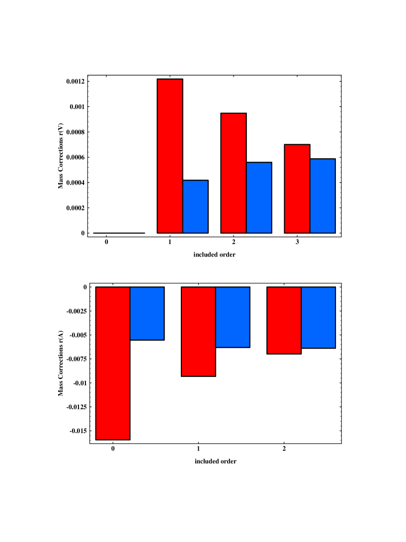
Figure 15: Mass Corrections from $r^{(1)}_{{\rm V}}$ (upper graph) and $r^{(1)}_{{\rm A}}$ (lower graph). The left-hand bars represent the result in the on-shell scheme, the right-hand ones are obtained in the $\overline{\mbox{MS}}$-scheme.

From the study of the stability of the prediction with respect to a variation of the renormalization scale an alternative error estimate can be deduced. It is obtained by using an equation equivalent to Eq. (198), but with arbitrary scale $\mu^{2}$ (see Appendix). In Fig. 16 the scale is varied between $\mu^{2}=s/4$ and $\mu^{2}=4s$. The corresponding error in the prediction for the decay rate amounts to $\delta\Gamma^{(m)}={+0.022\choose-0.006}$ MeV.

The uncertainty in the prediction from the input mass is essentially proportional to the relative error in $m^{2}$. Adopting $M_{{\rm b}}=4.7\pm 0.2\;{\rm GeV}$, one is lead to $\delta m^{2}/m^{2}\approx\pm 0.11$ and hence to a variation of the $m^{2}$ terms by $\pm 11\%$. It is clear that this contribution leads to the dominant error in the corrections corresponding to $\pm 0.17$ MeV. The combined uncertainty from mass term is therefore below $\delta\Gamma^{(m)}=\pm 0.21$ MeV.

Figure 16: Renormalization scale dependence of the massive axial QCD corrections; $[\alpha_{s}(M_{{Z}})=0.12]~{}.$

We now move to the massless limit. As discussed in Section 6.1 the reliability of the singlet terms is significantly improved through the inclusion of the $\alpha_{s}^{3}$ corrections. This is illustrated in Fig. 17, where the ${\cal O}(\alpha_{s}^{2})$ and ${\cal O}(\alpha_{s}^{3})$ predictions as functions of the renormalization scale are compared. From the variation of the full prediction an uncertainty $\delta\Gamma_{{\rm S}}={+0.12\choose-0.05}$ MeV can be deduced. (Taking the last calculated term of order $\alpha_{s}^{3}$ as an error estimate would lead to $\delta\Gamma_{{\rm S}}=\pm 0.25$ MeV. ) The singlet terms furthermore depend on the top mass. A change of our default value $M_{{\rm t}}=174$ GeV by $\pm 20$ GeV leads to a variation of $\delta\Gamma_{{\rm S}}$ by ${+0.10\choose-0.08}$ MeV.

Figure 17: Renormalization scale dependence of the axial singlet massless QCD corrections; $[\alpha_{s}(M_{{Z}})=0.12]$.

.

Figure 18: Renormalization scale dependence of the non-singlet massless QCD corrections. $[\alpha_{s}(M_{{Z}})=0.12]$

Clearly, even the combining linearly of the modulus of the three dominant errors (from the bottom mass, the singlet contribution and $M_{{\rm t}}$) leads to an uncertainty in the nonuniversal corrections of only ${+0.43\choose-0.33}$ MeV. This corresponds to an uncertainty in the value of $\alpha_{s}$ extracted from $\Gamma_{{\rm had}}$ of ${7.8\choose-6.2}\times 10^{-4}$ and a relative error in $\Gamma_{{\rm b}\overline{{\rm b}}}/\Gamma_{{\rm had}}$ of ${11\choose-9}\times 10^{-4}$, significantly below the anticipated experimental precision.

The remaining uncertainty in the $\alpha_{s}$ determination results from the unknown terms of ${\cal O}(\alpha_{s}^{4})$ in the non-singlet correction $r^{(0)}_{{\rm NS}}$. In Fig. 18 the variation of $r^{(0)}_{{\rm NS}}\equiv r_{1}$ with $\mu^{2}$ is displayed. Evidently one arrives at a fairly stable answer in order ${\cal O}(\alpha_{s}^{3})$. The variation of $\delta r^{(0)}_{{\rm NS}}={+0.4\choose-3.5}\times 10^{-4}$ may be interpreted as an error estimate. It translates into $\delta\Gamma^{(0)}={+0.07\choose-0.6}$ MeV and corresponds to an uncertainty in $\alpha_{s}$ of $\delta\alpha_{s}={+0.11\choose-1.05}\times 10^{-3}$.

This result is of course dependent on the input for $\alpha_{s}$. For central values of $\alpha_{s}=0.115$ and $\alpha_{s}=0.125$ one obtains $\delta\alpha_{s}={+0.11\choose-0.87}\times 10^{-3}$ and $\delta\alpha_{s}={+0.16\choose-1.26}\times 10^{-3}$ respectively. An alternative approach has been advocated in Ref. [110] (see also Ref. [111]), where an attempt is made to actually arrive at an estimate for the $(\alpha_{s}/\pi)^{4}$ term. Adopting their value for the coefficient of $-97$ one obtains a shift of $\delta r^{(0)}_{{\rm NS}}=-2.1\times 10^{-4}$ and hence of $\alpha_{s}$ by $-6.3\times 10^{-4}$, quite comparable to the error estimate presented above. As a third option one may again take the last calculated term in $\delta r^{(0)}_{{\rm NS}}$ for an error estimate, resulting in $\delta r^{(0)}_{{\rm NS}}=\pm 7.1\times 10^{-4}$ and $\delta\alpha_{s}=\pm 21.7\times 10^{-4}$. The choice is left to the reader.

7.1.2 The Partial Rate $\Gamma_{{\rm b}\overline{{\rm b}}}$

Another quantity of interest is the ratio $\Gamma_{{\rm b}\overline{{\rm b}}}/\Gamma_{{\rm had}}$. Assuming that ${\rm q\overline{q}}$ events with secondary radiation of ${\rm b}$ quarks (see Section 5.5) are assigned to $\Gamma_{{\rm q\overline{q}}}$, the universal QCD corrections $\Gamma_{{i}},\;i=1\dots 4$ cancel to a large extent and the nonuniversal parts dominate. Their contribution is small and the resulting uncertainty hence even smaller. The ratio can thus be predicted quite unambiguously. The near independence of the prediction on $\alpha_{s}$ is shown in Fig. 19. The flatness of the solid curve is the result of two (accidental) cancellations. With increasing $\alpha_{s}(M_{{Z}})$ the mass correction is lowered through the reduction of the running ${\rm b}$ mass (for fixed pole mass) the singlet correction, however, essentially increases proportional to $\alpha_{s}^{2}$. This is illustrated by the dashed curve, where the running mass has been kept fixed to the default value.

The deviation from the parton model prediction (with $m_{{\rm b}}=0$) amounts to 0.7% with a negligible error from higher-orders in $\alpha_{s}$. The uncertainties from the input values for $M_{{\rm b}}$ and $M_{{\rm t}}$ amount to $\pm 3\times 10^{-4}$ and $\pm 2\times 10^{-4}$ respectively.

Figure 19: The ratio $\displaystyle\Biggl{\{}\left({\Gamma_{{\rm b}\overline{{\rm b}}}}/{v_{{\rm b}}^{2}+a_{{\rm b}}^{2}}\right)/\left[{\Gamma_{{\rm had}}}/{\sum(v_{{f}}^{2}+a_{{f}}^{2})}\right]\Biggl{\}}$ versus $\alpha_{s}$. The dashed curve corresponds to a case of a fixed value of $m_{{\rm b}}(M_{{Z}})=2.77$ GeV, while the continuous one takes into account the implicit $\alpha_{s}$ dependence of $m_{{\rm b}}(M_{{Z}})$.

7.1.3 Quick Estimates

The previous formulae display the full dependence of the QCD corrections on the input parameters $m_{{\rm b}}$ and $M_{{\rm t}}$ as well as their effect on the vector and axial vector rate of the various quark species separately. These are the formulae most suited as building blocks for detailed fitting programs. It seems, however, also useful to provide a short numerical formula suited for quick estimates. For this purpose we set $m=\overline{m_{{\rm b}}}(M_{{Z}})=2.77~{}\pm$ 0.15 GeV (corresponding approximately to $M={m_{{\rm b}}|_{pole}}=4.7\pm 0.20$ GeV) and $M_{{\rm t}}|_{pole}=174~{}\pm$ 20 GeV. One obtains:

$$\frac{\Gamma_{{\rm had}}}{\Gamma_{0}} = 3\sum_{f}\displaystyle(v_{{f}}^{2}+a_{{f}}^{2})\Bigg{\{}1+\frac{\alpha_{s}}{\pi}+1.409\left(\frac{\alpha_{s}}{\pi}\right)^{2}-12.767\left(\frac{\alpha_{s}}{\pi}\right)^{3}$$

$$+(0.023\pm 0.005)\left(\frac{\alpha_{s}}{\pi}\right)^{2}+(-0.006\pm 0.001)\left(\frac{\alpha_{s}}{\pi}\right)^{3}\Bigg{\}}$$

$$+~{}3v_{{\rm b}}^{2}\Bigg{\{}\displaystyle(-5\times 10^{-6}\pm 1\times 10^{-6})+(0.011\pm 0.001)\frac{\alpha_{s}}{\pi}$$

$$\displaystyle+~{}(0.097\pm 0.01)\left(\frac{\alpha_{s}}{\pi}\right)^{2}+(0.51\pm 0.05)\left(\frac{\alpha_{s}}{\pi}\right)^{3}\Bigg{\}}$$

$$\displaystyle+~{}3\Bigg{\{}\displaystyle(-0.0055\pm 0.0006)+(-0.020\pm 0.002)\frac{\alpha_{s}}{\pi}$$

$$\displaystyle+~{}(-4.41\pm 0.26)\left(\frac{\alpha_{s}}{\pi}\right)^{2}+(-17.60\pm 0.30)\left(\frac{\alpha_{s}}{\pi}\right)^{3}\Bigg{\}}$$

$$\displaystyle+~{}3\left(\sum_{{f}}v_{{f}}\right)^{2}\Bigg{\{}-0.413\left(\frac{\alpha_{s}}{\pi}\right)^{3}\Bigg{\}}$$

$$\displaystyle+~{}3\sum_{{f}}(v_{{f}}^{2}+a_{{f}}^{2})Q_{{f}}^{2}\Bigg{\{}0.001867-0.000622\frac{\alpha_{s}}{\pi}\Bigg{\}}{}\,.$$

The origin of the terms is still evident from the structure of the couplings. For a simple evaluation of QCD corrections to the total rate one may now combine the correction coefficients with the numerically evaluated weights $v_{{\rm b}}^{2}/\sum_{{f}}(v_{{f}}^{2}+a_{{f}}^{2})$ etc. and arrive at

$$\Gamma_{{\rm had}}\displaystyle = \Gamma_{{\rm had}}\Bigg{|}_{{\scriptstyle m_{{\rm b}}=0\atop\scriptstyle\alpha_{s}=0}}\Bigg{\{}1+\frac{\alpha_{s}}{\pi}+1.40932\left(\frac{\alpha_{s}}{\pi}\right)^{2}-12.76706\left(\frac{\alpha_{s}}{\pi}\right)^{3}$$ (203)

$$-~{}(0.00040\pm 0.00008)-(0.0023\pm 0.0002)\frac{\alpha_{s}}{\pi}$$

$$-~{}(0.63\pm 0.04)\left(\frac{\alpha_{s}}{\pi}\right)^{2}$$

$$-~{}(2.69\pm+0.06)\left(\frac{\alpha_{s}}{\pi}\right)^{3}\Bigg{\}}{}\,.$$

A similar treatment of $\Gamma_{{\rm b}\overline{{\rm b}}}$ implies

$$\Gamma_{{\rm b}\overline{{\rm b}}} = \Gamma_{{\rm b}\overline{{\rm b}}}\Bigg{|}_{{\scriptstyle m_{{\rm b}}=0\atop\scriptstyle\alpha_{s}=0}}\Bigg{\{}1+\frac{\alpha_{s}}{\pi}+1.40932\left(\frac{\alpha_{s}}{\pi}\right)^{2}-12.76706\left(\frac{\alpha_{s}}{\pi}\right)^{3}$$

$$-~{}(0.0035\pm 0.0004)-(0.010\pm 0.001)\frac{\alpha_{s}}{\pi}$$

$$-~{}(2.95\pm 0.17)\left(\frac{\alpha_{s}}{\pi}\right)^{2}-(11.9\pm 0.3)\left(\frac{\alpha_{s}}{\pi}\right)^{3}\Bigg{\}}$$

and

$$\frac{\Gamma_{{\rm b}\overline{{\rm b}}}}{\Gamma_{{\rm had}}} = \left(\frac{\Gamma_{{\rm b}\overline{{\rm b}}}}{\Gamma_{{\rm had}}}\right)\Bigg{|}_{{\scriptstyle m_{{\rm b}}=0\atop\scriptstyle\alpha_{s}=0}}\Bigg{\{}1-(0.0031\pm 0.0003)-(0.005\pm 0.0005)\frac{\alpha_{s}}{\pi}$$ (205)

$$-~{}(2.3\pm 0.1)\left(\frac{\alpha_{s}}{\pi}\right)^{2}-(6.9\pm 0.3)\left(\frac{\alpha_{s}}{\pi}\right)^{3}\Bigg{\}}{}\,.$$

From these formulae it is evident that the coefficients of the $\alpha_{s}^{2}$ and the $\alpha_{s}^{3}$ terms are entirely different from the massless non-singlet case as a consequence of the bottom mass effects and virtual top loops discussed in this work. The deviation of this from 1 can be traced to two sources: the bottom mass term, responsible for the term independent of $\alpha_{s}$, and the singlet term mainly responsible for the $\alpha_{s}^{2}$ (and $\alpha_{s}^{3}$) contribution.

7.2 The Low-Energy Region
Near the Bottom Threshold

The previous discussion has dealt mainly with the applications of the theoretical results to the high energy region. However, as indicated already in Section 4.4 the results are also applicable for energies relatively close to the threshold of heavy quarks, if $m^{2}/s,m^{4}/s^{2}$ and $m^{6}/s^{3}$ terms are included. This was demonstrated for the Born and the $O(\alpha_{s})$ formulae in Section 4.4, where it was shown that these leading terms provide an excellent approximation even if the ratio $4m^{2}/s$ approaches $0.8$. With this justification a detailed analysis of $R_{{\rm had}}$ can be performed for the region above the charmonium resonances and below the bottom threshold (excluding, of course, the narrow $\Upsilon$ resonances). Furthermore the region above the $\overline{{\rm b}}{\rm b}$ resonances — say, above 11.5 or 12 GeV — can be treated in the same approximation.

With increasing statistics and precision at LEP the uncertainty in $\alpha_{s}$ from the measurement of the hadronic decay rate of the ${Z}$ can be reduced to $\pm 0.002$. It would be highly desirable to test the evolution of the strong coupling as predicted by the beta function through a determination of $\alpha_{s}$ from essentially the same observable — at lower energy, however. The region from several GeV above charm threshold (corresponding to the maximal energy of BEPC around $5.0$ GeV) to just below the $B$ meson threshold at around $10.5$ GeV (corresponding to the ‘off resonance’ measurements of CESR) seems particularly suited for this purpose. As a consequence of the favourable error propagation, the accuracy in the measurement (compared to $91$ GeV) may decrease by a factor of about three or even four at 10 and 5.6 GeV respectively, to achieve comparable precision in $\Lambda_{\overline{{\rm MS}}}$:

$$\delta\alpha_{s}(s)=\frac{\alpha_{s}^{2}(s)}{\alpha_{s}^{2}(M_{{Z}}^{2})}\delta\alpha_{s}(M_{{Z}}^{2})~{}.$$

Most of the results discussed above for massless quarks are applicable also for the case under consideration. However, two additional complications arise:

• Charm quark effects cannot be ignored completely and should be taken into consideration through an expansion in the ratio $m_{{\rm c}}^{2}/s$, employing the results of Sections 5.3 and 5.4 for terms of order $m_{{\rm c}}^{2}/s$ and $m_{{\rm c}}^{4}/s^{2}$.

• Contributions involving virtual bottom quarks are present, starting from order $\alpha_{s}^{2}$. Their contribution depends in a nontrivial manner on $m_{{\rm b}}^{2}/s$. In order $\alpha_{s}^{2}$ these are discussed in Section 5.2 and are shown to be small. Estimates for the corresponding contributions of order $\alpha_{s}^{3}$ indicate that they are under control and can be safely neglected, provided that one works within the correctly defined effective four-quark theory.

The results presented below are formulated for a theory with $n_{{f}}=4$ effective flavours and with the corresponding definitions of the coupling constant and the quark mass. The relation to a formulation with $n_{f}=5$ appropriate for the measurements above the ${\rm b}\bar{{\rm b}}$ threshold was discussed in Section 2.3 and will be given at the end of the paper.

We shall now list the independent contributions and their relative importance. Neglecting for the moment the masses of the charmed quark and a forteriori of the ${\rm u}$, ${\rm d}$ and ${\rm s}$ quarks one predicts in order $\alpha_{s}^{3}$,

$$R_{{\rm NS}}=\sum_{f={\rm u,d,s,c}}3Q_{{f}}^{2}\left[1+\frac{\alpha_{s}}{\pi}+1.5245\left(\frac{\alpha_{s}}{\pi}\right)^{2}-11.52033\left(\frac{\alpha_{s}}{\pi}\right)^{3}\right]$$ (206)

for the non-singlet contribution. The second and the third order coefficients are evaluated with $n_{{f}}=4$, which means that the bottom quark loops are absent. In order $\alpha_{s}^{2}$ the bottom quark loops can be taken into consideration with their full mass dependence given in Section 5.2. However, the leading term of order $\alpha_{s}^{2}/m_{{\rm b}}^{2}$ provides a fairly accurate description even up to the very threshold $s=4m_{{\rm b}}^{2}$. Hence one has to add a correction

$$\delta R_{m_{{\rm b}}}=\sum_{f={\rm u,d,s,c}}3Q_{{f}}^{2}\left(\frac{\alpha_{s}}{\pi}\right)^{2}\frac{s}{\bar{m}_{{\rm b}}^{2}}\left[\frac{44}{675}+\frac{2}{135}\ln\,\frac{\bar{m}_{{\rm b}}^{2}}{s}\right].$$ (207)

For the singlet term one obtains

$$R_{{\rm S}}=-\left(\frac{\alpha_{s}}{\pi}\right)^{3}\left(\sum_{{\rm u,d,s,c}}Q_{{f}}\right)^{2}\,1.239=-0.55091\left(\frac{\alpha_{s}}{\pi}\right)^{3}{}.$$ (208)

The bottom quark is absent in this sum. In view of the smallness of the $\alpha_{s}^{2}s/m^{2}_{{\rm b}}$ correction (even close to the ${\rm b}\bar{{\rm b}}$ threshold!) all other terms of ${\cal O}(\alpha_{s}^{3})$ from virtual ${\rm b}$ quarks are also neglected. This can be justified with the results of Ref. [39] where $s/m^{2}$ terms are evaluated. In the same spirit it is legitimate to use the scale invariant value of the ${\rm b}$ quark mass $\bar{m}_{{\rm b}}=\bar{m}_{{\rm b}}(\bar{m}^{2}_{{\rm b}})$ as defined in the five-quark theory.

In contrast to the bottom mass the effects of the charmed mass can be incorporated through an expansion in $m_{{\rm c}}^{2}/s$. Quadratic mass corrections are included up to order $\alpha_{s}^{3}$, quartic mass terms up to order $\alpha_{s}^{2}$. Since $m_{{\rm c}}^{2}/s$ is in itself a small expansion parameter, the order $\alpha_{s}^{2}m_{{\rm c}}^{4}/s^{2}$ terms should be sufficient for the present purpose.

The charmed mass corrections are thefore given by

$$\delta R_{m_{{\rm c}}} = 3\,Q_{{\rm c}}^{2}\,12\,\frac{m_{{\rm c}}^{2}}{s}~{}\frac{\alpha_{s}}{\pi}\left[1+9.097{}~{}\frac{\alpha_{s}}{\pi}+53.453\left(\frac{\alpha_{s}}{\pi}\right)^{2}\right]$$ (209)

$$-~{}3\sum_{f={\rm u,d,s,c}}Q_{{f}}^{2}~{}\frac{m_{{\rm c}}^{2}}{s}\left(\frac{\alpha_{s}}{\pi}\right)^{3}6.476$$

$$+{}~{}3\,Q_{{\rm c}}^{2}~{}\frac{m_{{\rm c}}^{4}}{s^{2}}\left\{-6-22~{}\frac{\alpha_{s}}{\pi}+\left[141.329-\frac{25}{6}\ln\,\left(\frac{m_{{\rm c}}^{2}}{s}\right)\right]\left(\frac{\alpha_{s}}{\pi}\right)^{2}\right\}$$

$$+~{}3\sum_{f={\rm u,d,s,c}}Q_{{f}}^{2}{}~{}\frac{m_{{\rm c}}^{4}}{s^{2}}\left(\frac{\alpha_{s}}{\pi}\right)^{2}\left[-0.4749-\ln\,\left(\frac{m_{{\rm c}}^{2}}{s}\right)\right]$$

$$-~{}3\,Q_{{\rm c}}^{2}~{}\frac{m_{{\rm c}}^{6}}{s^{3}}\left\{8+\frac{16}{27}{}~{}\frac{\alpha_{s}}{\pi}\left[6\ln\,\left(\frac{m_{{\rm c}}^{2}}{s}\right)+155\right]\right\}\,,$$

where $n_{{f}}=4$ has been adopted everywhere. Note that terms of order $\alpha_{s}^{3}m^{2}_{{\rm c}}/s$ are more important than those of order $\alpha_{s}^{2}m^{4}_{{\rm c}}/s^{2}$ in the whole energy region under consideration. For completeness, $m_{{\rm c}}^{6}/s^{3}$ and $\alpha_{s}m_{{\rm c}}^{6}/s^{3}$ terms are also listed, which, however, are insignificant and will be ignored in the numerical analysis.

The charm quark mass is to be taken as $m_{{\rm c}}=\bar{m}_{{\rm c}}^{(4)}(s)$ and is to be evaluated in the four-flavour theory via the standard RG equation with the initial value $\bar{m}_{{\rm c}}(\bar{m}_{{\rm c}})=1.12\ {\rm GeV}$, corresponding to a pole mass of $1.6$ GeV in the case of $\alpha_{s}^{(5)}(M_{{Z}})=0.120$ (see Section 2.4.2). A similar line of reasoning can be pursued for bottom mass terms in the region several GeV above the $B$ meson threshold. The formula given below is expected to provide a reliable answer for $\sqrt{s}$ around 15 GeV and perhaps even down to 13 GeV:

$$\delta R_{m} = 3~{}\left(Q_{{\rm c}}^{2}~{}\frac{m_{{\rm c}}^{2}}{s}+Q_{{\rm b}}^{2}~{}\frac{m_{{\rm b}}^{2}}{s}\right){}~{}12~{}\frac{\alpha_{s}^{(5)}}{\pi}\left[1+8.736~{}\frac{\alpha_{s}^{(5)}}{\pi}+45.657\left(\frac{\alpha_{s}^{(5)}}{\pi}\right)^{2}\right]$$ (210)

$$-~{}3\sum_{f={\rm u,d,s,c,b}}Q_{{f}}^{2}\left(\frac{m_{{\rm c}}^{2}}{s}+\frac{m_{{\rm b}}^{2}}{s}\right)\left(\frac{\alpha_{s}^{(5)}}{\pi}\right)^{3}6.126$$

$$+~{}3\,Q_{{\rm c}}^{2}~{}\frac{m_{{\rm c}}^{4}}{s^{2}}\left\{-6-22~{}\frac{\alpha_{s}^{(5)}}{\pi}+\left[139.489-\frac{23}{6}\ln\,\left(\frac{m_{{\rm c}}^{2}}{s}\right)+12~{}\frac{m_{{\rm b}}^{2}}{m_{{\rm c}}^{2}}\right]\left(\frac{\alpha_{s}^{(5)}}{\pi}\right)^{2}\right\}$$

$$+~{}3\,Q_{{\rm b}}^{2}~{}\frac{m_{{\rm b}}^{4}}{s^{2}}\left\{-6-22~{}\frac{\alpha_{s}^{(5)}}{\pi}+\left[139.489-\frac{23}{6}\ln\,\left(\frac{m_{{\rm b}}^{2}}{s}\right)+12~{}\frac{m_{{\rm c}}^{2}}{m_{{\rm b}}^{2}}\right]\left(\frac{\alpha_{s}^{(5)}}{\pi}\right)^{2}\right\}$$

$$+~{}3\sum_{f={\rm u,d,s,c,b}}Q_{{f}}^{2}~{}\frac{m_{{\rm c}}^{4}}{s^{2}}\left(\frac{\alpha_{s}^{(5)}}{\pi}\right)^{2}\left[-0.4749-\ln\,\left(\frac{m_{{\rm c}}^{2}}{s}\right)\right]$$

$$+~{}3\sum_{f={\rm u,d,s,c,b}}Q_{{f}}^{2}~{}\frac{m_{{\rm b}}^{4}}{s^{2}}\left(\frac{\alpha_{s}^{(5)}}{\pi}\right)^{2}\left[-0.4749-\ln\,\left(\frac{m_{{\rm b}}^{2}}{s}\right)\right]$$

$$-~{}3\,Q_{{\rm b}}^{2}~{}\frac{m_{{\rm b}}^{6}}{s^{3}}\left\{8+\frac{16}{27}{}~{}\frac{\alpha_{s}^{(5)}}{\pi}\left[6\ln\,\left(\frac{m_{{\rm b}}^{2}}{s}\right)+155\right]\right\}\,.$$

Above the $B$ meson threshold it is more convenient to express all quantities for $n_{{f}}=5$ theory and thus in (7.2) all the coupling constant and quark masses are evaluated in the five-flavour theory at the scale $\mu=\sqrt{s}$.

The transition from four- to five-flavour theory is performed as follows: The charm mass is naturally defined in the $n_{{f}}=4$ theory. In order to obtain the value of $m_{{\rm c}}=\bar{m}_{{\rm c}}^{(5)}(s)$ the initial value $\bar{m}_{{\rm c}}^{(4)}(1~{}{\rm GeV})$ is evolved via the $n_{{f}}=4$ RG equation to the point $\mu^{2}=M_{{\rm b}}^{2}$ and from there up to $\mu^{2}=s$, now, however, with the $n_{{f}}=5$ RG equation. The bottom mass, on the other hand, is naturally defined in the $n_{{f}}=5$ theory irrespective of the characteristic momentum scale of the problem under consideration. Hence we take $\overline{m}_{{\rm b}}(s)$ obtained from the scale invariant mass $\overline{m}_{{\rm b}}(\overline{m}_{{\rm b}})$ after running the latter with the help of the $n_{{f}}=5$ RG equation. Finally, $\alpha_{s}^{(4)}$ and $\alpha_{s}^{(5)}$ are related through the matching Eq. (99).

In Tables 4–7 the predictions for $R$ at $10.5$ and $13$ GeV are listed for different values of $\alpha_{s}^{(5)}(M_{{Z}})$ together with the values of $\alpha_{s}(s)$ and the running masses. Note that our predictions are presented without QED corrections from the running of $\alpha$ and from initial state radiation. Figure 20 shows the behaviour of the ratio $R(s)$ as a function of energy below and above the bottom threshold, for $\alpha_{s}(M_{{Z}})=0.120,0.125$ and $0.130$. The light quark ${\rm u,d,s,c}$) contribution is also displayed separately above $10.5$ GeV. It is evident that the predictions from the four- and five-flavour theories join smoothly. The additional contribution from the ${\rm b}\overline{{\rm b}}$ channel is presented down to $11.5$ GeV, where resonances start to contribute and the perturbative treatment necessarily ceases to apply.

Table 4

Values of $\Lambda^{(5)}_{\overline{{\scriptstyle MS}}},\ \Lambda^{(4)}_{\overline{{\scriptstyle MS}}},\ \alpha_{s}^{(4)}(s),\ m_{{\rm c}}^{(4)}(s)\ {\rm and}\ \overline{m}_{{\rm b}}(\overline{m}_{{\rm b}})$ at $\sqrt{s}=10.5$ GeV for different values of $\alpha_{s}^{(5)}(M_{{Z}}^{2})$.

$\alpha_{s}^{(5)}(M_{{Z}}^{2})$	$\Lambda^{(5)}_{\overline{{\rm MS}}}$	$\Lambda^{(4)}_{\overline{{\rm MS}}}$	$\alpha_{s}^{(4)}(s)$	$m_{{\rm c}}^{(4)}(s)$	$\overline{m}_{{\rm b}}(\overline{m}_{{\rm b}})$
0.1200	233 MeV	320 MeV	0.177	0.751 GeV	4.09 GeV
0.1250	302 MeV	403 MeV	0.188	0.637 GeV	4.03 GeV
0.1300	383 MeV	498 MeV	0.199	0.500 GeV	3.96 GeV

Table 5

Predictions for $R(s)$ at $\sqrt{s}=10.5$ GeV; the contributions to $\delta R_{m_{{\rm c}}}$ are shown separately for every power of the quark mass.

$\alpha_{s}^{(5)}(M_{{Z}}^{2})$	$R_{{\rm NS}}$	$R_{{\rm S}}$	$\delta R_{m^{2}_{{\rm c}}}$	$\delta R_{m^{4}_{{\rm c}}}$	$\delta R_{m_{{\rm b}}}$	$R$
0.1200	3.530	–0.000098	0.0077	–0.00023	0.0026	3.540
0.1250	3.543	–0.00012	0.0061	–0.000121	0.0030	3.551
0.1300	3.556	–0.00014	0.0041	–0.000046	0.0034	3.563

Table 6

Values of $\Lambda^{(5)}_{\overline{{\rm MS}}},\ \alpha_{s}^{(5)}(s),\ m_{{\rm c}}^{(5)}(s)\ {\rm and}\ m_{{\rm b}}^{(5)}(s)$ at $\sqrt{s}=13$ GeV for different values of $\alpha_{s}^{(5)}(M_{{Z}}^{2})$ .

$\alpha_{s}^{(5)}(M_{{Z}})$	$\Lambda^{(5)}_{\overline{{\rm MS}}}$	$\alpha_{s}^{(5)}(s)$	$m_{{\rm c}}^{(5)}(s)$	$m_{{\rm b}}^{(5)}(s)$
0.1200	233 MeV	0.172	0.729 GeV	3.41 GeV
0.1250	302 MeV	0.183	0.617 GeV	3.29 GeV
0.1300	383 MeV	0.194	0.483 GeV	3.17 GeV

Table 7

Predictions for $R(s)$ at $\sqrt{s}=13$ GeV; the contributions to $\delta R_{m}$ are shown separately for every power of the quark masses.

$\alpha_{s}^{(5)}(M_{{Z}}^{2})$	$R_{{\rm NS}}$	$R_{{\rm S}}$	$\delta R_{m^{2}}$	$\delta R_{m^{4}}$	$\delta R_{m^{6}}$	$R$
0.1200	3.875	–0.000023	0.023	–0.011	–0.0014	3.887
0.1250	3.888	–0.000027	0.023	–0.0092	–0.0011	3.901
0.1300	3.901	–0.000032	0.022	–0.0079	–0.00091	3.914

Figure 20: The ratio $R(s)$ below and above the ${\rm b}$ quark production threshold at $10.5$ GeV for $\alpha_{s}(M_{{Z}})=0.120,\,0.125$ and $0.130$. The contributions from light quarks are displayed separately.

Evidently the $b\overline{b}$ channel is present with full strength down to the resonance region — an important consequence of QCD corrections. From this discussion it should be evident that the theoretical prediction is well under control. Mass effects are small below the ${\rm b}\overline{{\rm b}}$ threshold as well as a few GeV above. An experimental test is of prime importance.

7.3 Conclusions

In this report we have tried to present, in a comprehensive form, the theoretical framework and all formulae presently available that are required to predict the QCD corrected total cross-section of ${\rm e}^{+}{\rm e}^{-}$ annihilation and the ${Z}$ decay rate into hadrons, with optimal accuracy. The presentation is supposed to be self-contained — and hopefully self-consistent — such that all formulae relevant for the prediction of experimental quantities can be deduced from this work without the need to combine results from different publications. Particular emphasis has been put on the influence of the non-vanishing bottom quark mass and on contributions from virtual top quarks, which are of particular importance for the so-called singlet contributions. Much of the discussion has been tailored for the 90 GeV region, wher experiments at LEP provide highly accurate data, but, applications to ‘low energies’, around 10 GeV or even lower, have been mentioned whenever appropriate.

The topic is approached from three different viewpoints: from the purely theoretical, laying the ground for the discussion, from the calculational, providing the formulae, and from the practical viewpoint, discussing the relative importance of the various contributions and associated uncertainties. In the first two parts the basis of the subsequent calculations is presented. They contain, essentially, a brief review of the field theoretical ingredients: $\beta$ function and anomalous dimensions, the relations between various definitions of the mass, the decoupling of heavy quarks, and the corresponding transitions between different ‘effective theories’. In many circumstances quarks are either light ($m^{2}\ll s$) or heavy ($m^{2}\gg s$). The corresponding expansions provide powerful tools. They are described in Part 2.

The results of higher-order calculations are scattered in numerous original publications, often with conflicting conventions and notations. In Parts 3, 5 and 6 the formulae are collected and presented in a uniform way. The brief presentation of exact results of $O(\alpha_{s})$ (i.e. with arbitrary $m^{2}/s$) in Part 4 leads quickly to Parts 5 and 6 where $m^{2}/s$ or $s/m^{2}$ are treated as expansion parameters, and results of up to order $\alpha_{s}^{3}$ are collected. An important classification of amplitudes originates from the distinction between singlet and non-singlet diagrams, with markedly different behaviour in the limit $m^{2}/s\gg 1$, and our presentation follows this classification. Whilst most of the discussion is concerned with predictions for the total cross-section or the decay rate, occasionally also results for partial rates, for example into four fermion states or for the inclusive rate into ${\rm b}\bar{{\rm b}}$ quarks, are presented. The formulae are displayed in two different forms: first in analytical form with the relevant coefficients given by fractions and Riemann’s Zeta function, as functions of $n_{f}$, and then entirely numerically (Part 7 and the Appendices) in terms of decimal fractions.

The final Part is most relevant to practical applications. The numerical relevance (or irrelevance) of the various contributions is clarified. Their stability with respect to variations of the renormalization scale $\mu$ is studied. Estimates are presented for the errors from the truncation of the perturbation series, the ‘theoretical error’, and for the error induced by the uncertainty in the input parameters $M_{{\rm b}}$ and $M_{{\rm t}}$. A safe upper limit on the combined uncertainty of $\Gamma(Z\to{\rm hadrons})$ from quark mass ($M_{{\rm b}}$ and $M_{{\rm t}}$) dependent corrections amounts to about $0.4$ MeV. The uncertainty from the truncation of the perturbative expansion in the massless limit in $O(\alpha_{s}^{3})$ is highly subjective, with estimates ranging from $0.6$ MeV up to $1.2$ MeV. Fortunately enough, in the foreseeable future, both sources of errors will not effect the precision of $\alpha_{s}$ as determined at LEP through total cross-section measurements.

For the convenience of the reader, simple numerical formulae are presented which allow a quick estimate of $\Gamma_{{\rm had}}$ , $\Gamma_{{\rm b}\bar{{\rm b}}}$ and their ratio. A similar discussion for the energy region around the bottom threshold concludes this Part. For easy access the formulas most frequently used in practical applications are collected and rewritten in the Appendices.

Acknowledgements

We would like to thank our collaborators A. Hoang, M. Jeżabek, B. Kniehl, D. Pirjol, K. Schilcher, O. Tarasov, T. Teubner and P. Zerwas for providing important input and essential ingredients to this report. We have benefitted from helpful and clarifying discussions with G. Passarino. We are grateful to M. Steinhauser for reading the manuscript and help with drawing some figures. The review would not have been completed without the encouragement and initiative provided by the LEP study group, in particular by Dima Bardin.

We are indebted to W. Bernreuther, T. Hebbeker, W. Hollik, A. Kataev, B. Kniehl and P. Zerwas for reading the manuscript and providing us with their comments and corrections.

Over the past years this work has been supported by the Deutsche Forschungsgemeinschaft (grants Ku 502/3-1, Ku 502/6-1), by the Bundesministerium für Forschung und Technologie (contracts 005KA94P1, 056KA93P), and by the HERAEUS-Stiftung. K. Chetyrkin thanks the Universität Karlsruhe for a guest professorship and the Institute of Theoretical Particle Physics for the warm hospitality extended to him during recent years. His work was partially supported by the Russian Fund of the Fundamental Research (grant 93-02-14428). A. Kwiatkowski thanks the Deutsche Forschungsgemeinschaft for financial support (grant no. Kw 8/1-1). Partial support by US DoE under Contract DE-AC03-76SF00098 is gratefully acknowledged.

Appendixes

1 Some Useful Formulae

Zeta function

The Riemann Zeta function is defined by

$$\zeta(s)=\sum_{k=1}^{\infty}k^{-s}{}\,.$$ (1)

Some particular values are:

$$\begin{array}[]{ll}\displaystyle\zeta(0)=-~{}\frac{1}{2}~{},&\displaystyle\quad\zeta(2)=\frac{\pi^{2}}{6}=1.6449341~{},\\ \displaystyle\zeta(3)=1.2020569~{},&\quad\zeta(4)=\frac{\pi^{4}}{90}=1.0823232~{},\\ \zeta(5)=1.0369278~{}.\par&\end{array}.$$ (2)

Dilogarithm

$$\mbox{Li}_{2}(x)=\sum_{n=1}^{\infty}\frac{x^{2}}{n^{2}}~{},\ \ \ \ \ \ (|x|<1){}$$ (3)

or

$$\mbox{Li}_{2}(x)=-\int_{0}^{x}\frac{\ln\,(1-t)}{t}~{}{\rm dt}{}\,.$$ (4)

2 Renormalization Group Functions

The RG equation for the quark mass reads:

$$\mu^{2}\frac{d}{d\mu^{2}}\bar{m}(\mu)=\bar{m}(\mu)\gamma_{m}\equiv-\bar{m}(\mu)\sum_{i\geq 0}\gamma_{m}^{i}\left(\frac{\alpha_{s}}{\pi}\right)^{i+1}.$$ (1)

It is solved by

$$\begin{array}[]{rl}\displaystyle\bar{m}(\mu)=&\displaystyle\bar{m}(\mu_{0})\exp\,\left\{\frac{1}{\pi}\int^{\alpha_{s}(\mu)}_{\alpha_{s}(\mu_{0})}{\rm d}x\frac{\gamma_{m}(x)}{\beta(x)}\right\}\\ =&\displaystyle\bar{m}(\mu_{0})\left[\frac{\alpha_{s}(\mu)}{\alpha_{s}(\mu_{0})}\right]^{{\gamma_{m}^{0}}/{\beta_{0}}}\left\{1+\left(\frac{\gamma_{m}^{1}}{\beta_{0}}-\frac{\beta_{1}\gamma_{m}^{0}}{\beta_{0}^{2}}\right)\left[\frac{\alpha_{s}(\mu)}{\pi}-\frac{\alpha_{s}(\mu_{0})}{\pi}\right]\right.\\ &\displaystyle+~{}\frac{1}{2}\left(\frac{\gamma_{m}^{1}}{\beta_{0}}-\frac{\beta_{1}\gamma_{m}^{0}}{\beta_{0}^{2}}\right)^{2}\left[\frac{\alpha_{s}(\mu)}{\pi}-\frac{\alpha_{s}(\mu_{0})}{\pi}\right]^{2}\\ &\displaystyle\left.+~{}\frac{1}{2}\left(\frac{\gamma_{m}^{2}}{\beta_{0}}-\frac{\beta_{1}\gamma_{m}^{1}}{\beta_{0}^{2}}-\frac{\beta_{2}\gamma_{m}^{0}}{\beta_{0}^{2}}+\frac{\beta_{1}^{2}\gamma_{m}^{0}}{\beta_{0}^{3}}\right)\left[\left(\frac{\alpha_{s}(\mu)}{\pi}\right)^{2}-\left(\frac{\alpha_{s}(\mu_{0})}{\pi}\right)^{2}\right]\right\}.\end{array}$$ (2)

with

$$\begin{array}[]{ll}\displaystyle\gamma_{m}^{0}&=\displaystyle 1,\ \ \ \gamma_{m}^{1}=\left(\frac{202}{3}-\frac{20}{9}~{}n_{f}\right)/16,\\[12.91663pt] \displaystyle\gamma_{m}^{2}&=\displaystyle\left\{1249-\left[\frac{2216}{27}+\frac{160}{3}\zeta(3)\right]n_{f}-\frac{140}{81}~{}n_{f}^{2}\right\}/64{}\,.\end{array}$$ (3)

Similarly, one has for the strong coupling constant ($L\equiv\ln\,\mu^{2}/\Lambda^{2}_{\overline{{\rm MS}}}$):

$$\mu^{2}\frac{d}{d\mu^{2}}\left[\frac{\alpha_{s}(\mu)}{\pi}\right]=\beta\equiv-\sum_{i\geq 0}\beta_{i}\left(\frac{\alpha_{s}}{\pi}\right)^{i+2},$$ (4)

Integration gives

$$\frac{\alpha_{s}(\mu)}{\pi}=\frac{1}{\beta_{0}L}\left\{1-\frac{1}{\beta_{0}L}\frac{\beta_{1}\ln\,L}{\beta_{0}}+\frac{1}{\beta_{0}^{2}L^{2}}\left[\frac{\beta_{1}^{2}}{\beta_{0}^{2}}(\ln^{2}L-\ln\,L-1)+\frac{\beta_{2}}{\beta_{0}}\right]\right\},$$ (5)

with

$$\begin{array}[]{ll}\displaystyle\beta_{0}&=\displaystyle\left(11-\frac{2}{3}~{}n_{f}\right)/4,\;\;\;\;\beta_{1}=\left(102-\frac{38}{3}~{}n_{f}\right)/16~{},\\[12.91663pt] \displaystyle\beta_{2}&=\displaystyle\left(\frac{2857}{2}-\frac{5033}{18}~{}n_{f}+\frac{325}{54}~{}n_{f}^{2}\right)/64{}\,~{}.\end{array}$$ (6)

3 List of Radiative Corrections

In this section all contributions to the total hadronic ${Z}$ decay rate are collected. Complete order $\alpha_{s}$ prediction with full mass dependence ($v^{2}=1-4m^{2}/s$):

$$\Gamma_{{\rm had}} = \Gamma_{0}3\Bigg{\{}\sum_{f}v_{f}^{2}v\frac{3-v^{2}}{2}\left[1+\frac{4}{3}\frac{\displaystyle\alpha_{s}(s)}{\displaystyle\pi}K_{{\rm V}}\right]$$ (1)

$$+\sum_{f}a_{f}^{2}v^{3}\left[1+\frac{4}{3}\frac{\displaystyle\alpha_{s}(s)}{\displaystyle\pi}K_{{\rm A}}\right]\Bigg{\}}{}\,,$$

with

$$\begin{array}[]{ll}K_{{\rm V}}=&\displaystyle\frac{1}{v}\left[A(v)+\frac{P_{{\rm V}}(v)}{(1-v^{2}/3)}\ln\,\frac{1+v}{1-v}+\frac{Q_{{\rm V}}(v)}{(1-v^{2}/3)}\right],\\ \displaystyle K_{{\rm A}}=&\displaystyle\frac{1}{v}\left[A(v)+\frac{P_{{\rm A}}(v)}{v^{2}}\ln\,\frac{1+v}{1-v}+\frac{Q_{{\rm A}}(v)}{v^{2}}\right]{}\,,\end{array}$$ (2)

and

$$\begin{array}[]{ll}\displaystyle A(v)=&\displaystyle(1+v^{2})\left\{{\rm Li}_{2}\left[\left(\frac{1-v}{1+v}\right)^{2}\right]+2{\rm Li}_{2}\left(\frac{1-v}{1+v}\right)+\ln\,\frac{1+v}{1-v}\ln\,\frac{(1+v)^{3}}{8v^{2}}\right\}\\ &\displaystyle+~{}3v\ln\,\frac{1-v^{2}}{4v}-v\ln\,v{}\,,\end{array}$$ (3)

$$\begin{array}[]{ll}\displaystyle P_{{\rm V}}(v)=\frac{33}{24}+\frac{22}{24}v^{2}-\frac{7}{24}v^{4}{}\,,&\displaystyle\quad Q_{{\rm V}}(v)=\frac{5}{4}v-\frac{3}{4}v^{3}{}\,,\\ \displaystyle P_{{\rm A}}(v)=\frac{21}{32}+\frac{59}{32}v^{2}-\frac{19}{32}v^{4}-\frac{3}{32}v^{6}~{},&\;\;\;\;\displaystyle Q_{{\rm A}}(v)=-~{}\frac{21}{16}v+\frac{30}{16}v^{3}+\frac{3}{16}v^{5}{}\,,\end{array}$$ (4)

where $\Gamma_{0}=G_{F}M_{Z}^{3}/24\sqrt{2}\pi=82.94$ MeV.

Including higher-order corrections the decay rate can be written in the following form:

$$\Gamma_{{\rm had}}=\sum_{i=1}^{12}\Gamma_{i}=\sum_{i=1}^{12}\Gamma_{0}R_{i}{}\,~{}.$$ (5)

The separate contributions are given by the following expressions. [Below in Eqs. (6–15) $\alpha_{s}$, $\overline{m}_{f}$ and $\overline{m}_{b}$ stand for $\alpha^{(5)}_{s}(\mu)$, $\overline{m}_{f}^{(5)}(\mu)$ and $\overline{m}_{b}^{(5)}(\mu)$ respectively.] Massless non-singlet corrections:

$$R_{1} = 3\sum_{f}(v_{f}^{2}+a_{f}^{2})\Bigg{\{}1+\frac{\alpha_{s}}{\pi}$$ (6)

$$+\left(\frac{\alpha_{s}}{\pi}\right)^{2}\left[\frac{365}{24}-11\zeta(3)+~{}n_{f}\left(-~{}\frac{11}{12}+\frac{2}{3}\zeta(3)\right)+\left(-~{}\frac{11}{4}+\frac{1}{6}n_{f}\right)\ln\,\frac{s}{\mu^{2}}\right]$$

$$+\left(\frac{\alpha_{s}}{\pi}\right)^{3}\Bigg{[}\frac{87029}{288}-\frac{121}{48}\pi^{2}-\frac{1103}{4}\zeta(3)+\frac{275}{6}\zeta(5)$$

$$+~{}n_{f}\left(-~{}\frac{7847}{216}+\frac{11}{36}\pi^{2}+\frac{262}{9}\zeta(3)-\frac{25}{9}\zeta(5)\right)+n_{f}^{2}\left(\frac{151}{162}-\frac{1}{108}\pi^{2}-\frac{19}{27}\zeta(3)\right)$$

$$+\left(-~{}\frac{4321}{48}+\frac{121}{2}\zeta(3)+~{}n_{f}\left[\frac{785}{72}-\frac{22}{3}\zeta(3)\right]+~{}n_{f}^{2}\left[-\frac{11}{36}+\frac{22}{3}\zeta(3)\right]\right)\ln\,\frac{s}{\mu^{2}}$$

$$+\left(\frac{121}{16}-\frac{11}{12}n_{f}+\frac{1}{36}n_{f}^{2}\right)\ln^{2}\frac{s}{\mu^{2}}\Bigg{]}\Bigg{\}}$$

$$= 3\sum_{f}(v_{f}^{2}+a_{f}^{2})\Bigg{\{}1+\frac{\alpha_{s}}{\pi}$$

$$+\left(\frac{\alpha_{s}}{\pi}\right)^{2}\left[1.9857-0.1152~{}n_{f}+\left(-2.75+0.167~{}n_{f}\right)\ln\,\frac{s}{\mu^{2}}\right]$$

$$+\left(\frac{\alpha_{s}}{\pi}\right)^{3}\Bigg{[}-6.6369-1.2001~{}n_{f}-0.0052~{}n_{f}^{2}$$

$$+\left(-17.2964+2.0877~{}n_{f}-0.0384~{}n_{f}^{2}\right)\ln\,\frac{s}{\mu^{2}}$$

$$+\left(7.5625-0.9167~{}n_{f}+0.0278~{}n_{f}^{2}\right)\ln^{2}\frac{s}{\mu^{2}}\Bigg{]}\Bigg{\}}{}\,;$$

Massive universal corrections (‘double bubble’):

$$R_{2} = 3\sum_{f}(v_{f}^{2}+a_{f}^{2})\left(\frac{\alpha_{s}}{\pi}\right)^{3}\sum_{f^{\prime}=b}\frac{\overline{m}_{f^{\prime}}^{2}}{s}\Bigg{\{}-80+60\zeta(3)+n_{f}\left[\frac{32}{9}-\frac{8}{3}\zeta(3)\right]\Bigg{\}}$$

$$= 3\sum_{f}(v_{f}^{2}+a_{f}^{2})\left(\frac{\alpha_{s}}{\pi}\right)^{3}\sum_{f^{\prime}=b}\frac{\overline{m}_{f^{\prime}}^{2}}{s}\Bigg{\{}-7.8766+0.3501~{}n_{f}\Bigg{\}}$$

$$R_{3} = 3\sum_{f}(v_{f}^{2}+a_{f}^{2})\left(\frac{\alpha_{s}}{\pi}\right)^{2}\sum_{f^{\prime}=b}\frac{\overline{m}_{f^{\prime}}^{4}}{s^{2}}\left\{\frac{13}{3}-4\zeta(3)-\ln\,\frac{\overline{m}_{f^{\prime}}^{2}}{s}\right\}$$

$$= 3\sum_{f}(v_{f}^{2}+a_{f}^{2})\left(\frac{\alpha_{s}}{\pi}\right)^{2}\sum_{f^{\prime}=b}\frac{\overline{m}_{f^{\prime}}^{4}}{s^{2}}\left\{-0.4749-\ln\,\frac{\overline{m}_{f^{\prime}}^{2}}{s}\right\}$$

$$R_{4} = 3\sum_{f}(v_{f}^{2}+a_{f}^{2})\left(\frac{\alpha_{s}}{\pi}\right)^{2}\frac{s}{M_{{\rm t}}^{2}}\left\{\frac{44}{675}+\frac{2}{135}\ln\,\frac{M_{{\rm t}}^{2}}{s}\right\}$$ (7)

$$= 3\sum_{f}(v_{f}^{2}+a_{f}^{2})\left(\frac{\alpha_{s}}{\pi}\right)^{2}\frac{s}{M_{{\rm t}}^{2}}\left\{0.0652+0.0148\ln\,\frac{M_{{\rm t}}^{2}}{s}\right\}{}\,;$$

Massive non-singlet corrections (vector):

$$R_{5} = 3v_{{\rm b}}^{2}~{}\frac{\overline{m}_{{\rm b}}^{2}}{s}\Bigg{\{}12\frac{\alpha_{s}}{\pi}+\left(\frac{\alpha_{s}}{\pi}\right)^{2}\left[\frac{253}{2}-\frac{13}{3}~{}n_{f}+(-57+2~{}n_{f})\ln\,\frac{s}{\mu^{2}}\right]$$ (8)

$$+\left(\frac{\alpha_{s}}{\pi}\right)^{3}\Bigg{[}2522-\frac{285}{4}~{}\pi^{2}+\frac{310}{3}~{}\zeta(3)-\frac{5225}{6}~{}\zeta(5)$$

$$+~{}n_{f}\left(-~{}\frac{4942}{27}+\frac{17}{3}~{}\pi^{2}-\frac{394}{27}~{}\zeta(3)+\frac{1045}{27}~{}\zeta(5)\right)+n_{f}^{2}\left(\frac{125}{54}-\frac{1}{9}~{}\pi^{2}\right)$$

$$+\left(-~{}\frac{4505}{4}+\frac{175}{2}~{}n_{f}-\frac{13}{9}~{}n_{f}^{2}\right)\ln\,\frac{s}{\mu^{2}}+\left(\frac{855}{4}-17~{}n_{f}+\frac{1}{3}~{}n_{f}^{2}\right)\ln^{2}\frac{s}{\mu^{2}}\Bigg{]}\Bigg{\}}$$

$$= 3v_{{\rm b}}^{2}~{}\frac{\overline{m}_{{\rm b}}^{2}}{s}\Bigg{\{}12~{}\frac{\alpha_{s}}{\pi}+\left(\frac{\alpha_{s}}{\pi}\right)^{2}\left[126.5-4.3333~{}n_{f}+(-57+2~{}n_{f})\ln\,\frac{s}{\mu^{2}}\right]$$

$$+\left(\frac{\alpha_{s}}{\pi}\right)^{3}\Bigg{[}1040.01-104.517~{}n_{f}+1.2182~{}n_{f}^{2}$$

$$+\left(-1126.25+87.5~{}n_{f}-1.4444~{}n_{f}^{2}\right)\ln\,\frac{s}{\mu^{2}}$$

$$+\left(213.75-17~{}n_{f}+0.3333~{}n_{f}^{2}\right)\ln^{2}\frac{s}{\mu^{2}}\Bigg{]}\Bigg{\}}$$

$$\displaystyle R_{6}\displaystyle = 3v_{{\rm b}}^{2}~{}\frac{\overline{m}_{{\rm b}}^{4}}{s^{2}}\Bigg{\{}-6+\frac{\alpha_{s}}{\pi}\left[-22+24\ln\frac{s}{\mu^{2}}\right]$$ (9)

$$+\left(\frac{\alpha_{s}}{\pi}\right)^{2}\Bigg{[}-\frac{3029}{12}+27~{}\pi^{2}+112~{}\zeta(3)-\frac{11}{2}\ln\,\frac{\overline{m}_{{\rm b}}^{2}}{s}+225\ln\frac{s}{\mu^{2}}-81\ln^{2}\frac{s}{\mu^{2}}$$

$$+~{}n_{f}\left(\frac{143}{18}-\frac{2}{3}~{}\pi^{2}-\frac{8}{3}\zeta(3)+\frac{1}{3}\ln\,\frac{\overline{m}_{{\rm b}}^{2}}{s}-\frac{22}{3}\ln\frac{s}{\mu^{2}}+2\ln^{2}\frac{s}{\mu^{2}}\right)\Bigg{]}\Bigg{\}}$$

$$= 3v_{{\rm b}}^{2}~{}\frac{\overline{m}_{{\rm b}}^{4}}{s^{2}}\Bigg{\{}-6+\frac{\alpha_{s}}{\pi}\left[-22+24\ln\frac{s}{\mu^{2}}\right]$$

$$+\left(\frac{\alpha_{s}}{\pi}\right)^{2}\Bigg{[}148.693-5.5\ln\,\frac{\overline{m}_{{\rm b}}^{2}}{s}+255\ln\frac{s}{\mu^{2}}-81\ln^{2}\frac{s}{\mu^{2}}$$

$$+{}~{}n_{f}\left(-1.8408+0.3333\ln\,\frac{\overline{m}_{{\rm b}}^{2}}{s}-7.3333\ln\frac{s}{\mu^{2}}+2\ln^{2}\frac{s}{\mu^{2}}\right)\Bigg{]}\Bigg{\}}{}\,;$$

Massive non-singlet corrections (axial):

$$R_{7}\displaystyle = 3~{}\frac{\overline{m}_{{\rm b}}^{2}}{s}\Bigg{\{}-6+\frac{\alpha_{s}}{\pi}\left[-22+12\ln\,\frac{s}{\mu^{2}}\right]$$

$$+\left(\frac{\alpha_{s}}{\pi}\right)^{2}\Bigg{[}-\frac{8221}{24}+\frac{19}{2}~{}\pi^{2}+117~{}\zeta(3)+n_{f}\left(\frac{151}{12}-\frac{1}{3}~{}\pi^{2}-4~{}\zeta(3)\right)$$

$$+\left(155-\frac{16}{3}~{}n_{f}\right)\ln\,\frac{s}{\mu^{2}}+\left(-~{}\frac{57}{2}+n_{f}\right)\ln^{2}\frac{s}{\mu^{2}}\Bigg{]}\Bigg{\}}$$

$$= 3~{}\frac{\overline{m}_{{\rm b}}^{2}}{s}\Bigg{\{}-6+\frac{\alpha_{s}}{\pi}\left[-22+12\ln\,\frac{s}{\mu^{2}}\right]$$

$$+\left(\frac{\alpha_{s}}{\pi}\right)^{2}\Bigg{[}-108.14+4.4852~{}n_{f}+\left(155-5.3333~{}n_{f}\right)\ln\,\frac{s}{\mu^{2}}+\left(-28.5+n_{f}\right)\ln^{2}\frac{s}{\mu^{2}}\Bigg{]}\Bigg{\}}$$

$$\displaystyle R_{8}\displaystyle = 3~{}\frac{\overline{m}_{{\rm b}}^{4}}{s^{2}}\Bigg{\{}6+\frac{\alpha_{s}}{\pi}\left[10-24\ln\frac{s}{\mu^{2}}\right]$$ (11)

$$+\left(\frac{\alpha_{s}}{\pi}\right)^{2}\Bigg{[}\frac{3389}{12}-27~{}\pi^{2}-220~{}\zeta(3)+\frac{77}{2}\ln\,\frac{\overline{m}_{{\rm b}}^{2}}{s}-207\ln\frac{s}{\mu^{2}}+81\ln^{2}\frac{s}{\mu^{2}}$$

$$+~{}n_{f}\left(-~{}\frac{41}{6}+\frac{2}{3}~{}\pi^{2}+\frac{16}{3}~{}\zeta(3)-\frac{7}{3}\ln\,\frac{\overline{m}_{{\rm b}}^{2}}{s}+\frac{22}{3}\ln\frac{s}{\mu^{2}}-2\ln^{2}\frac{s}{\mu^{2}}\right)\Bigg{]}\Bigg{\}}$$

$$= 3~{}\frac{\overline{m}_{{\rm b}}^{4}}{s^{2}}\Bigg{\{}6~{}\frac{\alpha_{s}}{\pi}\left[10-24\ln\frac{s}{\mu^{2}}\right]$$

$$+\left(\frac{\alpha_{s}}{\pi}\right)^{2}\Bigg{[}-248.515+38.5\ln\,\frac{\overline{m}_{{\rm b}}^{2}}{s}-207\ln\frac{s}{\mu^{2}}+81\ln^{2}\frac{s}{\mu^{2}}$$

$$+{}~{}n_{f}\left(6.1574-2.3333\ln\,\frac{\overline{m}_{{\rm b}}^{2}}{s}+7.3333\ln\frac{s}{\mu^{2}}-2\ln^{2}\frac{s}{\mu^{2}}\right)\Bigg{]}\Bigg{\}}{}\,;$$

Singlet corrections (axial):

$$R_{9}\displaystyle = \left(\frac{\alpha_{s}}{\pi}\right)^{2}\left\{-9.250+1.037\frac{s}{4M_{{\rm t}}^{2}}+0.632\left(\frac{s}{4M_{{\rm t}}^{2}}\right)^{2}+3\ln\,\frac{s}{M_{{\rm t}}^{2}}\right\}$$ (12)

$$+\left(\frac{\alpha_{s}}{\pi}\right)^{3}\Bigg{\{}-\frac{5075}{72}+\frac{23}{12}~{}\pi^{2}+3~{}\zeta(3)+\frac{67}{6}\ln\,\frac{\mu^{2}}{M_{{\rm t}}^{2}}$$

$$+~{}\frac{23}{4}\ln^{2}\frac{\mu^{2}}{M_{{\rm t}}^{2}}+\frac{373}{8}\ln\,\frac{s}{\mu^{2}}-\frac{23}{4}\ln^{2}\frac{s}{\mu^{2}}\Bigg{\}}$$

$$= \left(\frac{\alpha_{s}}{\pi}\right)^{2}\left\{-9.250+1.037~{}\frac{s}{4M_{{\rm t}}^{2}}+0.632\left(\frac{s}{4M_{{\rm t}}^{2}}\right)^{2}+3\ln\,\frac{s}{M_{{\rm t}}^{2}}\right\}$$

$$+\left(\frac{\alpha_{s}}{\pi}\right)^{3}\Bigg{\{}-47.963+11.167\ln\,\frac{\mu^{2}}{M_{{\rm t}}^{2}}$$

$$+~{}5.75\ln^{2}\frac{\mu^{2}}{M_{{\rm t}}^{2}}+46.625\ln\,\frac{s}{\mu^{2}}-5.75\ln^{2}\frac{s}{\mu^{2}}\Bigg{\}}$$

$$R_{10}\displaystyle = 3\left(\frac{\alpha_{s}}{\pi}\right)^{2}\left\{-6\frac{\overline{m}^{2}_{{\rm b}}}{s}\left[-3+\ln\,\frac{s}{M_{{\rm t}}^{2}}\right]-~{}10\frac{\overline{m}^{2}_{{\rm b}}}{M_{{\rm t}}^{2}}\left[\frac{8}{81}-\frac{1}{54}\ln\,\frac{s}{M_{{\rm t}}^{2}}\right]\right\}{}\,;$$ (13)

Singlet corrections (vector):

$$R_{11}=\left(\sum_{f}v_{f}\right)^{2}\left(\frac{\alpha_{s}}{\pi}\right)^{3}(-1.2395){}\,;$$ (14)

${\cal O}(\alpha\alpha_{s})$ corrections:

$$R_{12}=3\sum_{f}(v_{f}^{2}+a_{f}^{2})Q_{f}^{2}~{}\frac{3}{4}{}~{}\frac{\alpha}{\pi}\left[1-\frac{1}{3}~{}\frac{\alpha_{s}}{\pi}\right]{}\,;$$ (15)

$R_{{\rm had}}$ from virtual photons: The prediction for the ‘classical’ production through a value $R^{{\rm em}}=\sigma({\rm e}^{+}{\rm e}^{-}\mathrel{\mathop{\kern 0.0pt\to}\limits_{\gamma}}\mbox{hadrons})/\sigma_{{\rm point}}$ is obtained from the above equations by setting $a_{f}=0$ and $R^{{\rm em}}=\sum_{1}^{6}R_{i}$ after setting $v_{f}\to Q_{f}$ and $a_{f}\to 0$;

Secondary radiation of heavy quarks: The rate for secondary radiation of a pair of quarks with mass $m$ is given by

$$\frac{\Gamma_{{{\rm Q}\overline{{\rm Q}}{\rm q}\overline{{\rm q}}}}}{\Gamma_{{\rm q}\overline{{\rm q}}}}=\frac{2}{3}\left(\frac{\alpha_{s}}{\pi}\right)^{2}\varrho^{R}\left(\frac{m^{2}}{s}\right){}\,,$$ (16)

where

$$\varrho^{R}(x) = \frac{4}{3}\,\left(1-6x^{2}\right)\,\left\{\frac{1}{2}\,{\rm Li}_{3}\left({{1-w}\over 2}\right)-\frac{1}{2}\,{\rm Li}_{3}\left({{1+w}\over 2}\right)\right.$$ (17)

$$\left.+\,{\rm Li}_{3}\left({{1+w}\over{1+a}}\right)-{\rm Li}_{3}\left({{1-w}\over{1-a}}\right)+{\rm Li}_{3}\left({{1+w}\over{1-a}}\right)-{\rm Li}_{3}\left({{1-w}\over{1+a}}\right)\right.$$

$$+\,\frac{1}{2}\,\ln\,\left({{1+w}\over{1-w}}\right)\left[\zeta(2)-\frac{1}{12}\,\ln^{2}\left(\frac{1+w}{1-w}\right)\right.$$

$$+\frac{1}{2}\,\ln^{2}\left(\frac{a-1}{a+1}\right)-\left.\left.\frac{1}{2}\,\ln\,\left(\frac{1+w}{2}\right)\ln\,\left(\frac{1-w}{2}\right)\right]\right\}$$

$$+\,\frac{1}{9}\,a\,\left(19+46x\right)\,\left[{\rm Li}_{2}\left({{1+w}\over{1+a}}\right)+{\rm Li}_{2}\left({{1-w}\over{1-a}}\right)-{\rm Li}_{2}\left({{1+w}\over{1-a}}\right)-{\rm Li}_{2}\left({{1-w}\over{1+a}}\right)\right.$$

$$\left.+\,\ln\,\left({{a-1}\over{a+1}}\right)\,\ln\,\left({{1+w}\over{1-w}}\right)\right]$$

$$+\,4\left({{19}\over{72}}+x+x^{2}\right)\,\left[{\rm Li}_{2}\left(-~{}\frac{1+w}{1-w}\right)-{\rm Li}_{2}\left(-~{}\frac{1-w}{1+w}\right)-\ln\,x\,\ln\,\left(\frac{1+w}{1-w}\right)\right]$$

$$+\,7\left({{73}\over{189}}+{{74}\over{63}}x+x^{2}\right)\,\ln\,\left({{1+w}\over{1-w}}\right)-\,\frac{1}{3}\left({{2123}\over{108}}+\frac{2489}{54}x\right)\,w\,,$$

with

$$a=\sqrt{1+4x}\,,\quad w=\sqrt{1-4x}~{}.$$

References

• [1] D. Schaile, Precision Tests of the Electroweak Interaction, XXVII Intern.  Conference on HEP, Glasgow, 1994.
• [2] T. Hebbeker, Phys. Rep. 217 (1992) 69; Z. Hioki, Mod. Phys. Lett. A7 (1992) 1009; W. Hollik, in Advanced Series on Directions in High Energy Physics—Vol. 10: Heavy Flavours, ed. by A.J. Buras and M. Lindner (World Scientific, Singapore, 1994), p. 1; W. Hollik and A. Sirlin, to appear in Advanced Series on Directions in High Energy Physics: Precision Tests of the Standard Electroweak Model, ed. by P. Langacker (World Scientific, Singapore, 1994); S. Bethke, to appear in Proceedings of the Tennessee International Symposium on Radiative Corrections: Status and Outlook, Gatlinburg, Tennessee, June 27–July 1, 1994, ed. by B.F.L. Ward (World Scientific, Singapore, 1994); B.A. Kniehl, Preprint KEK–TH–412 (September 1994), to appear in Int. J. Mod. Phys. A.
• [3] S. Adler, Phys. Rev. D10 (1974) 3714.
• [4] E.C. Poggio, H.R.Quinn, S.Weinberg, Phys. Rev. D 13 (1976) 1958.
• [5] N.N. Bogoliubov and D.V. Shirkov, Introduction to the theory of the quantized fields, 4th supplemented edition (Nauka, Moscow, 1984).
• [6] J.C. Collins, Renormalization (Cambridge University Press, 1984).
• [7] C. Itzykson and J. Zuber, Quantum Field Theory (McGraw Hill, New York, 1980).
• [8] F.J. Ynduráin, The Theory of Quarks and Gluon Interactions , (Springer-Verlag, Berlin, 1994).
• [9] G.’t Hooft and M. Veltman, Nucl.  Phys. B 44 (1972) 189.
• [10] C.G. Bollini and J.J. Giambiagi, Phys. Let. 40B (1972) 566;
G.M. Cicuta and E.Montaldi, Nuovo Cim. Lett. 4 (1972) 329;
J.F. Ashmore, Nuovo Cim. Lett. 4 (1972) 289.
• [11] G. ’t Hooft, Nucl. Phys. B 61 (1973) 455 .
• [12] W.A. Bardeen, A.J. Buras, D.W. Duke and T. Muta, Phys.  Rev. D18 (1978) 3998.
• [13] W.A. Caswell and A.D. Kennedy, Phys. Rev. D 25 (1982) 392.
• [14] O.V. Tarasov, A.A. Vladimirov, A.Yu. Zharkov, Phys. Lett. B 93 (1980) 429.
• [15] O.V. Tarasov, preprint JINR P2-82-900 (1982).
• [16] S.A. Larin and J.A.M. Vermaseren, Phys. Lett. B 303 (1993) 334.
• [17] S.A. Larin, Preprint NIKHEF-H/92-18, hep-ph/9302240 (1992); In Proc. of the Int. Baksan School ”Particles and Cosmology” (April 22-27, 1993, Kabardino-Balkaria, Russia) eds. E.N. Alexeev, V.A. Matveev, Kh.S. Nirov, V.A. Rubakov (World Scientific, Singapore, 1994).
• [18] G. Grunberg, Phys. Lett. B 221 (1980) 70; Phys. Rev. D29 (1984) 2315.
• [19] P.M. Stevenson, Phys. Rev. D23 (1981) 2916.
• [20] N.V. Krasnikov, A.L.Kataev and A.A. Pivovarov, Nucl. Phys. B 198 (1982) 508.
• [21] J. Kubo and S. Sakakibara, Z. Phys. C14 (1982) 345.
• [22] A. Dhar and V. Gupta, Phys. Rev. D29 (1984) 2822;
V. Gupta, D.V. Shirkov and O.V. Tarasov, Int. J. Mod. Phys. A6 (1991) 3381.
• [23] S. Brodsky, G.P. Lepage and P.B. Mackenzie, Phys. Rev. D28 (1983) 228;
Hung Jung Lu, Phys. Rev. D45 (1992) 1217.
• [24] I.I. Bigi, M.A. Shifman, N.G. Uraltsev, and A.I. Vainshtein, Preprint TPI-MINN-94/4-T, CERN-TH.7171/94, UND-HEP-94-BIG (1994).
• [25] P. Binetruy and T. Sücker, Nucl. Phys. B 178 (1981) 293.
• [26] R. Coquereaux, Ann. Phys. 125 (1980) 407
• [27] R. Tarrach, Nucl. Phys. B 183 (1981) 384.
• [28] S. Narison, Phys. Lett. B 197 (187) 405.
• [29] N.Gray, D.J.Broadhurst, W.Grafe and K.Schilcher, Z. Phys. C 48 (1990) 673.
• [30] D.J.Broadhurst, N.Gray, and K. Schilcher, Z. Phys. C 52 (1991) 111.
• [31] J.C. Collins, Nucl. Phys. B 92 (1975) 477.
• [32] K.G.Chetyrkin, J.H.Kühn, A.Kwiatkowski, Phys.  Lett. B 282 (1992) 221.
• [33] S.G.Gorishny, A.L.Kataev, S.A.Larin, L.R.Surguladze, Mod. Phys. Lett. A 5 (1990) 2703.
• [34] T. Appelquist and J. Carazzone, Phys.  Rev. D 11 (1975) 2856.
• [35] S. Weinberg, Phys. Lett. B 91 (1980) 51.
• [36] B.A. Ovrut and H.J. Schnitzer, Phys. Lett. 100B (1981) 403.
• [37] W. Bernreuther, W. Wetzel, Nucl. Phys. B 197 (1982) 228.
• [38] W. Bernreuther, Ann. Phys. 151 (1983) 127.
• [39] S.A. Larin, T. van Ritbergen and J.A.M. Vermaseren, Preprint NIKHEF-H/94-30 (1994).
• [40] K.G. Chetyrkin, Phys.  Lett. B 307 (1993) 169.
• [41] J. Collins, F. Wilczek and A. Zee, Phys.   Rev. D18 (1978) 242;
• [42] K.G. Chetyrkin and J.H. Kühn, Z. Phys. C60 (1993) 497.
• [43] K.G. Chetyrkin and J.H. Kühn, Phys. Lett. B 308 (1993) 127.
• [44] V.A. Novikov, M.A. Shifman, A.I. Vainstein and V.I. Zakharov, Fortschr. Phys. 32 (1984) 585.
• [45] S. Narison, Preprint CERN-TH.7277/94 and PM 94/11 (1994).
• [46] S. Narison, Preprint CERN-TH.7405/94 (1994).
• [47] J. Bijnens, J. Prades and E. de Rafael, Preprint CTP-94/PE.3097 and NORDITA - 94/62 N,P, November 1994.
• [48] M. Jamin and M. Münz, Preprint CERN-TH.7435/94 and TUM-T31-78/94, September 1994.
• [49] K.G. Chetyrkin, C.A. Dominguez, D. Pirjol and K. Schilcher, Preprint MZ-TH/94-21 and UCT-TP 214/94, August 1994.
• [50] J. Gasser and H. Leutwyler, Phys. Rep. 87 (1987) 77.
• [51] C.A. Dominguez and E. de Rafael, Ann. Phys. 174 (1987) 372.
• [52] S. Narison, Phys. Lett. B 216 (1989) 191.
• [53] C.A. Domingues and N. Paver, Phys. lett. B 293 (1992) 197.
• [54] S. Titard and F.J. Yndurain, Phys. Rev. D49 (1994) 6007.
• [55] Electroweak Precision Calculation Working Group, D. Bardin, private communication.
• [56] CDF Collaboration, F. Abe et al., Phys. Rev. Lett. 73 (1994) 225.
• [57] D.J. Broadhurst and S.C. Generalis, Open University report No. OUT-4102-12 (1984) (unpublished).
• [58] K.Chetyrkin and K.G.Spiridonov, Sov. J. Nucl. Phys. 47, (1988) 522.
• [59] D.J. Broadhurst and S.C. Generalis, Open University report No. OUT-4102-22 (1988) (unpublished).
• [60] D.J.Broadhurst, Phys. Lett. B 101 , 423 (1981).
• [61] S.C. Generalis, J. Phys. G: Nucl. Part. Phys. 15, (1989) L225.
• [62] K.G. Chetyrkin, S.G. Gorishny and F.V. Tkachov, Phys. Lett. B 119, 407 (1982).
• [63] V.P. Spiridonov, preprint INR P-0378 (1984).
• [64] K.G. Chetyrkin and J.H. Kühn, Nucl. Phys. B 432 (1994) 337.
• [65] G.B. Pivovarov, F.V. Tkachov, Preprint INR P-0370 (1984), Moscow;
F.V. Tkachov, Int. Journ. Mod. Phys. A 8 (1993) 2047;
G.B. Pivovarov, F.V. Tkachov, Int. Journ. Mod. Phys. A 8 (1993) 2241.
• [66] S.G.Gorishny, S.A.Larin, Nucl. Phys. B 287 (1987) 452;
S.G. Gorishny, Nucl. Phys. B 319 (1989) 633.
• [67] K.G. Chetyrkin, V.A. Smirnov, Preprint INR P-518 (1987), Moscow;
K.G. Chetyrkin, Preprint MPI-PAE/PTh 13/91 (1991), Munich;
V.A. Smirnov, Commun. Math. Phys. 134 (1990) 109.
• [68] V.A. Smirnov, Renormalization and Asymptotic Expansion, (Birkhäuser, Basel, 1991).
• [69] P. Breitenlohner, D. Maison, Comm. Math. Phys. V.52 (1977) 11.
• [70] D.A. Akyeampong and R. Delbourgo, Nuovo Cimento 17A (1973) 578.
• [71] T.L. Trueman, Phys. Lett. B 88 (1979) 331.
• [72] S.A. Larin and J.A.M. Vermaseren, Phys. Lett. B 259 (1991) 345.
• [73] S.A. Larin, Phys. Lett. B 303 (1993) 113; Preprint NIKHEF-H/92-19 (1992).
• [74] D.J. Broadhurst and A.L. Kataev, Phys. Lett. B 315 (1993) 179.
• [75] J. Schwinger, Particles, Sources and Fields, Vol.II, (Addison-Wesley, New York, 1973).
• [76] J. Jersak, E. Laermann and P.M. Zerwas, Phys. Lett. B 98 (1981) 363; Phys.  Rev.  D25 (1982) 1218.
• [77] T.H. Chang, K.J.F. Gaemers and W.L. van Neerven, Nucl. Phys. B 202 (1980) 407.
• [78] B.A.Kniehl, J.H.Kühn, Nucl. Phys. B 329 (1990) 547.
• [79] S. Güsken, J.H. Kühn and P. Zerwas, Phys. Lett. B 155 (1985) 185.
• [80] J.H. Kühn and P. Zerwas, Phys. Rep. 167 (1988) 360.
• [81] V.S. Fadin and V.A. Khoze, JETP Lett. 46 (1987) 525,
• [82] J.M. Strassler and M.E. Peskin, Phys. Rev. D43 (1991) 1500.
• [83] J.H. Kühn, M. Jeżabek and T. Teubner, Z. Phys. C 56 (1992) 653.
• [84] M. Jeżabek and T. Teubner, Z. Phys. C 59 (1993) 669.
• [85] Y. Sumino et al. Phys. Rev. D 47 (1993) 56.
• [86] J.H. Kühn, A. Djouadi and P.M. Zerwas, Z. Phys. C 46 (1990) 412.
• [87] K.G.Chetyrkin, J.H.Kühn, Phys. Lett. B 248 (1990) 359.
• [88] K.G. Chetyrkin, A.L. Kataev, F.V. Tkachov, Phys. Lett.  B 85 (1979) 277;
M. Dine, J. Sapirstein, Phys. Rev. Lett. 43 (1979) 668;
W. Celmaster, R.J. Gonsalves, Phys. Rev. Lett. 44 (1980) 560.
• [89] S.G. Gorishny, A.L. Kataev, S.A. Larin, Phys. Lett. B 212 (1988) 238.
• [90] S.G. Gorishny, A.L. Kataev, S.A. Larin, Phys. Lett. 259 (1991) 144;
• [91] L.R. Surguladze and M.A. Samuel, Phys. Rev. Lett. 66 (1991) 560 and 2416 (Erratum).
• [92] A.L.Kataev, Phys. Lett. B 287 (1992) 209.
• [93] B.A. Kniehl, Phys. Lett. B 237 (1990) 127.
• [94] A.H Hoang, M. Jeżabek, J.H. Kühn and T. Teubner, Phys. Lett. B 338 (1994) 330.
• [95] W. Bernreuther and W. Wetzel, Z. Phys.  11 (1981) 113.
• [96] W. Wetzel and W. Bernreuther, Phys.Rev. D24 (1982) 2724.
• [97] D.E. Soper and L.R. Surguladze, Phys. Rev. Lett. 73 (1994) 2958.
• [98] S.G. Gorishny, A.L. Kataev, S.A. Larin, Nuovo Cimento 92 (1986) 117.
• [99] K.G. Chetyrkin and A. Kwiatkowski, Z. Phys. C59 (1993) 525.
• [100] L.R. Surguladze, Preprint INR P-0644, Moscow (1989) (unpublished)
• [101] L.R. Surguladze, Preprint OITS-554 (1994).
• [102] M.H. Seymor, Z. Phys. C63 (1994) 99; Preprint LU-TP-94-7 (1994).
• [103] B.A. Kniehl, J.H. Kühn, Phys. Lett. B 224 (1990) 229.
• [104] L.D. Landau, Dokl. Akad. Nawk, USSR 60 (1948) 207; C.N. Yang, Phys. Rev. 77 (1949) 242.
• [105] K.G. Chetyrkin and A. Kwiatkowski, Phys. Lett. B 319 (1993) 307.
• [106] K.G. Chetyrkin and O.V. Tarasov, Phys. Lett. B 327 (1994) 114;
S.A. Larin, T. van Ritbergen and J.A.M. Vermaseren, Phys. Lett. B 320 (1994) 159.
• [107] K.G. Chetyrkin and A. Kwiatkowski, Phys. Lett. B 305 (1993) 285.
• [108] R. Höpker, J.J. van der Bij, Phys. Rev. D 49 (1994) 3779.
• [109] S. Fanchiotti, B. Kniehl and A. Sirlin, Phys. Rev. D 48 (1993) 307.
• [110] A.L. Kataev and V.V. Starshenko, preprint CERN-TH.7400/94 (1994); Mod. Phys. Lett. A, to appear.
• [111] J. Bjorken, Preprint SLAC-PUB-5103; Proc. Cargese Summer Institute (1989).
• [112] K.G. Chetyrkin and J.H. Kühn, Phys. Lett. B 342 (1995) 356.