1. Introduction

The supersymmetric theories now stand as the most promising candidate for the unified theory beyond the standard model [1]. The supersymmetry helps to resolve the gauge hierarchy problem [2]. Moreover, the accurate data favor remarkably the supersymmetric grand unified theory (GUT) over the nonsupersymmetric theory [3]. This fact has fulfilled the promise that accurate measurements of coupling constant strengths at low energies can distinguish various alternative candidates for the grand unified theories by extrapolating the renormalization group trajectories to higher energies.

Among many problems in particle physics, the violation of $CP$ invariance is one of the phenomena that are least understood. The primary reason for this unsatisfactory situation is that the experimental verification of the $CP$ violation is so far limited to neutral Kaon dacays into two pions. We expect to obtain more experimental informations on the $CP$ violation from the B-factory soon. The $CP$ violation is not only important as a fundamental symmetry property, but also needed to explain the cosmological baryon asymmetry of our universe [4]. Therefore it is most desirable to have additional experimental informations on the $CP$ violation. Apart from the forthcoming experiment with the B-factory, we have one more promising observable for the $CP$ violation: the electric dipole moment (EDM), in particular those of neutron and electron [5]. Since we can hope for further improvements of experimental precision, especially for that of neutron, we expect that the EDM will provide a precious clue of the $CP$ violation. The $CP$ violation in the minimal standard model arises solely from the Cabibbo-Kobayashi-Maskawa matrix of the Yukawa coupling constants of the Higgs field. Therefore progress in the study of the $CP$ violation provides important informations on the Higgs field which is most elusive in the standard model.

In supersymmetric models, we have more possibilities for complex parameters beside the Cabibbo-Kobayashi-Maskawa matrix, even if we have only the minimal particle content of the supersymmetric standard model. These complex parameters become additional sources of the $CP$ violation. Among the parameters of the supersymmetric models, those associated with the soft breaking of supersymmetry are least understood. The early studies of the EDM in supersymmetric models have revealed that generic complex parameters for the soft breaking give too large EDM unless superpartners in the loop are heavier than at least a few TeV [6]. Although this type of models are not excluded, it is perhaps more attractive and natural if we can control the phases of the soft breaking parameters so that superpartner masses of the order of the electroweak scale are naturally allowed. There have been many studies on this issue [7, 8].

In the most popular model, the supergravity with the hidden sector provides a definite pattern of the soft breaking of supersymmetry [1, 9]. If we assume a simple model for the hidden sector and the supergravity couplings, we obtain that these parameters are real at the grand unification scale or the Planck scale. However, the soft breaking parameters that are really manifest at low energies will become complex since nonvanishing phases will be induced by the renormalization group flow involving the Cabibbo-Kobayashi-Maskawa matrix [10, 5]. Moreover, flavor-changing couplings of gluino are also induced [11]. This radiative effect becomes important when the Yukawa couplings are large. It is worth examining the $CP$ violation due to this radiatively induced phases of the soft breaking parameters, since it is now certain that the top quark is quite heavy [12] and requires a large Yukawa coupling.

More recently, there have been a number of studies on the neutron EDM in the supersymmetric models [13] or in two Higgs doublet models [14].

In the nonsupersymmetric minimal standard model, it has been proposed that the transition quark EDM can be more important than the single quark EDM to explain the neutron EDM [15, 16, 17].

The purpose of this paper is to examine the neutron electric dipole moment in the minimal supersymmetric standard model. We assume that there are complex parameters only in the Cabibbo-Kobayashi-Maskawa matrix at the grand unification scale. We examine the effect of the radiatively induced phases of the soft supersymmetry breaking parameters on the neutron EDM. In performing the renormalization group analysis, we have taken account of the effect of gaugino masses together with the universal scalar masses. We shall also consider the transition quark EDM in the supersymmetric models. We find that the single quark EDM is of the order of $10^{-27}\sim 10^{-29}\>e\cdot$cm for the light chargino mass to be 50 GeV. We also find that the transition EDM is of the order of $10^{-25}\sim 10^{-27}\>e\cdot$cm and hence contributes the neutron EDM of the order of $10^{-29}\sim 10^{-31}\>e\cdot$cm, if we take account of the large QCD enhancement due to the penguin diagrams. In both cases, the neutron EDM in this class of models is too small to be detected in forthcoming experiments.

In sect. 2, we introduce soft breaking parameters of supersymmetry and scalar particle mass matrices. In sect. 3, we analyze the single quark EDM. There are two classes of contributions: the chargino loop and the gluino loop. In sect. 4, we examine the transition EDM. Appendix is devoted to describe our results of the renormalization group equations and our inputs.

2. Soft breaking parameters of supersymmetry

We consider the minimal supersymmetric standard model (MSSM) which contains left-chiral supermultiplets for three generations of quarks ($\mbox{\boldmath$U$}^{c}$, $\mbox{\boldmath$D$}^{c}$, $Q$) and leptons ($\mbox{\boldmath$E$}^{c}$, $L$), gauge bosons of the SU$(3)_{\rm c}\times$SU$(2)_{\rm L}\times$U$(1)_{Y}$ and two Higgs doublets ($H_{u}$, $H_{d}$). Boldface letters such as $Q$ denote vectors in generation indices, and the suffix $c$ denotes the antiparticle. The supergravity with the hidden sector provides the pattern of the soft breaking of supersymmetry [1, 9]. In simple models of this type, the soft breaking parameters are real and universal at the grand unification (GUT) scale or the Planck scale, and a complex phase appears only in the Cabibbo-Kobayashi-Maskawa matrix at the scale. Renormalization group running induces complex phases in the soft breaking parameters at the lower scale.

One can write superpotential of MSSM as follows,

$$-W\equiv\mbox{\boldmath$U$}^{cT}\mbox{\boldmath$Y$}_{u}H_{u}\cdot\mbox{\boldmath$Q$}-\mbox{\boldmath$D$}^{cT}\mbox{\boldmath$Y$}_{d}H_{d}\cdot\mbox{\boldmath$Q$}-\mbox{\boldmath$E$}^{cT}\mbox{\boldmath$Y$}_{e}H_{d}\cdot\mbox{\boldmath$L$}+\mu H_{u}\cdot H_{d},$$ (2.1)

where boldface letters $Y$ are Yukawa couplings as a matrix in generation indices. The inner product of SU(2) indices is abbreviated by the $\cdot$ as $H_{u}\cdot H_{d}\equiv(i\sigma_{2}H_{u})^{T}H_{d}$.

Soft supersymmetry breaking is given by the following terms in the Lagrangian:

1. scalar mass terms,

   $$-\sum_{i,j}m_{ij}^{2}\phi_{i}^{*}\phi_{j}$$ (2.2)

   The $\phi_{i}$’s are all the scalar particles and $m_{ij}^{2}$ is a hermitian matrix. In the supergravity-induced models, this will be universal at the GUT scale, i.e., $m_{ij}^{2}=m^{2}\delta_{ij}$ at the GUT scale. It runs by renormalization group flow.

2. $A$ terms (trilinear scalar couplings),

   $$-\tilde{\mbox{\boldmath$u$}}_{R}^{\dagger}\mbox{\boldmath$A$}_{u}h_{u}\cdot\tilde{\mbox{\boldmath$q$}}_{L}+\tilde{\mbox{\boldmath$d$}}_{R}^{\dagger}\mbox{\boldmath$A$}_{d}h_{d}\cdot\tilde{\mbox{\boldmath$q$}}_{L}+\tilde{\mbox{\boldmath$e$}}_{R}^{\dagger}\mbox{\boldmath$A$}_{e}h_{d}\cdot\tilde{\mbox{\boldmath$\ell$}}_{L}+{\rm H.c.}$$ (2.3)

   In the supergravity-induced models, $A$’s are proportional to Yukawa couplings at the GUT scale, $\mbox{\boldmath$A$}=A\mbox{\boldmath$Y$}$. The $A$ terms run by renormalization group flow.

3. $B$ term,

   $$B\mu h_{u}\cdot h_{d}+{\rm H.c.}$$ (2.4)

4. gaugino mass terms,

   $$-\sum_{i=1}^{3}M_{i}\overline{\lambda_{iR}}\lambda_{iL}+{\rm H.c.}$$ (2.5)

   If GUT is embedded in the supergravity-induced models, $M_{i}$ ($i=1,2,3$) are universal, i.e., $M_{i}=M$ at the GUT scale. Gaugino masses $M_{i}$ run by renormalization group flow.

We can write scalar-quark mass terms in the following form:

$$-\left(\!\!\begin{array}[]{cc}\tilde{\mbox{\boldmath$u$}}_{L}^{\dagger}&\tilde{\mbox{\boldmath$u$}}_{R}^{\dagger}\end{array}\!\!\right)\>M_{\tilde{u}}^{2}\left(\!\!\begin{array}[]{c}\tilde{\mbox{\boldmath$u$}}_{L}\\ \tilde{\mbox{\boldmath$u$}}_{R}\end{array}\!\!\right)-\left(\!\!\begin{array}[]{cc}\tilde{\mbox{\boldmath$d$}}_{L}^{\dagger}&\tilde{\mbox{\boldmath$d$}}_{R}^{\dagger}\end{array}\!\!\right)\>M_{\tilde{d}}^{2}\left(\!\!\begin{array}[]{c}\tilde{\mbox{\boldmath$d$}}_{L}\\ \tilde{\mbox{\boldmath$d$}}_{R}\end{array}\!\!\right),$$ (2.6)

where $\tilde{\mbox{\boldmath$u$}}_{L,R}$ ($\tilde{\mbox{\boldmath$d$}}_{L,R}$) is a u-type-scalar-quark (d-type-scalar-quark) field column vector in generation indices.

Denoting the scalar-quark mass matrices at the GUT scale with the suffix $0$, one can find

$$M_{\tilde{u}0}^{2} = \left(\!\!\begin{array}[]{cc}m_{\tilde{u}L}^{2}{\bf 1}+\mbox{\boldmath$M$}_{u}^{\dagger}\mbox{\boldmath$M$}_{u}&(A+\mu\cot\beta)\mbox{\boldmath$M$}_{u}^{\dagger}\\ \mbox{\boldmath$M$}_{u}(A+\mu\cot\beta)&m_{\tilde{u}R}^{2}{\bf 1}+\mbox{\boldmath$M$}_{u}\mbox{\boldmath$M$}_{u}^{\dagger}\end{array}\!\!\right),$$ (2.9)

$$M_{\tilde{d}0}^{2} = \left(\!\!\begin{array}[]{cc}m_{\tilde{d}L}^{2}{\bf 1}+\mbox{\boldmath$M$}_{d}^{\dagger}\mbox{\boldmath$M$}_{d}&(A+\mu\tan\beta)\mbox{\boldmath$M$}_{d}^{\dagger}\\ \mbox{\boldmath$M$}_{d}(A+\mu\tan\beta)&m_{\tilde{d}R}^{2}{\bf 1}+\mbox{\boldmath$M$}_{d}\mbox{\boldmath$M$}_{d}^{\dagger}\end{array}\!\!\right),$$ (2.12)

where $\mbox{\boldmath$M$}_{u}$ and $\mbox{\boldmath$M$}_{d}$ are matrices in generation indices for u-type and d-type quark masses respectively and are given by Yukawa couplings $Y$ and vacuum expectation values $v$ of Higgs fields,

$$\mbox{\boldmath$M$}_{u}=\mbox{\boldmath$Y$}_{u}\frac{v_{u}}{\sqrt{2}}, \mbox{\boldmath$M$}_{d}=\mbox{\boldmath$Y$}_{d}\frac{v_{d}}{\sqrt{2}}.$$ (2.13)

The $\tan\beta$ is defined as $v_{u}/v_{d}$. The generation independent part of the scalar-quark masses are given by the universal mass and the contribution from the $D$-term [18]:

$$m_{\tilde{u}L}^{2} = m^{2}-M_{Z}^{\ 2}(-\cos 2\beta)\left(\frac{1}{2}-\frac{2}{3}\sin^{2}\theta_{W}\right),$$ (2.14)

$$m_{\tilde{u}R}^{2} = m^{2}-\frac{2}{3}M_{Z}^{\ 2}(-\cos 2\beta)\sin^{2}\theta_{W},$$ (2.15)

$$m_{\tilde{d}L}^{2} = m^{2}+M_{Z}^{\ 2}(-\cos 2\beta)\left(\frac{1}{2}-\frac{1}{3}\sin^{2}\theta_{W}\right),$$ (2.16)

$$m_{\tilde{d}R}^{2} = m^{2}+\frac{1}{3}M_{Z}^{\ 2}(-\cos 2\beta)\sin^{2}\theta_{W}.$$ (2.17)

In writing the above formulas, we assumed for simplicity a universal form of the supersymmetry breaking, namely the universal scalar mass $m$ and the trilinear scalar coupling with the universal parameter $A$. Moreover, all the parameters are real except the Yukawa coupling constants which appear in the quark mass matrices at the GUT scale. Therefore the Yukawa couplings or the Cabibbo-Kobayashi-Maskawa matrix is the only source of $CP$ violation in this model at the GUT scale.

The renormalization group flow changes these scalar-quark mass matrices at the lower scale [19]. At the lower scale, these mass matrices can be written as follows:

$$M_{\tilde{u}}^{2} = \left(\!\!\begin{array}[]{cc}m_{\tilde{u}L}^{2}{\bf 1}+\mbox{\boldmath$M$}_{u}^{\dagger}\mbox{\boldmath$M$}_{u}+\mbox{\boldmath$\delta m$}_{\tilde{u}L}^{2}&(\mbox{\boldmath$A$}_{u}+\mu\cot\beta{\bf 1})\mbox{\boldmath$M$}_{u}^{\dagger}\\ \mbox{\boldmath$M$}_{u}(\mbox{\boldmath$A$}_{u}^{\dagger}+\mu\cot\beta{\bf 1})&m_{\tilde{u}R}^{2}{\bf 1}+\mbox{\boldmath$M$}_{u}\mbox{\boldmath$M$}_{u}^{\dagger}+\mbox{\boldmath$\delta m$}_{\tilde{u}R}^{2}\end{array}\!\!\right),$$ (2.20)

$$M_{\tilde{d}}^{2} = \left(\!\!\begin{array}[]{cc}m_{\tilde{d}L}^{2}{\bf 1}+\mbox{\boldmath$M$}_{d}^{\dagger}\mbox{\boldmath$M$}_{d}+\mbox{\boldmath$\delta m$}_{\tilde{d}L}^{2}&(\mbox{\boldmath$A$}_{d}+\mu\tan\beta{\bf 1})\mbox{\boldmath$M$}_{d}^{\dagger}\\ \mbox{\boldmath$M$}_{d}(\mbox{\boldmath$A$}_{d}^{\dagger}+\mu\tan\beta{\bf 1})&m_{\tilde{d}R}^{2}{\bf 1}+\mbox{\boldmath$M$}_{d}\mbox{\boldmath$M$}_{d}^{\dagger}+\mbox{\boldmath$\delta m$}_{\tilde{d}R}^{2}\end{array}\!\!\right),$$ (2.23)

where $\mbox{\boldmath$\delta m$}^{2}$’s are hermitian matrices defined from the soft SUSY breaking scalar mass parameters which are determined from the renormalization group flow and have off-diagonal elements at the electroweak scale. After the renormalization group running, the parameter $A$’s become matrices in generation indices and the left-left (LL) and right-right (RR) blocks have off-diagonal elements. The off-diagonal terms of the matrices $A$’s turn out to be important for the neutron EDM. We show the renormalization group equations and their solutions for the matrices $A$’s in Appendix A.

It is convenient to rotate the scalar-quark wave functions by the same amount as to diagonalize the mass matrices of the quarks themselves, although scalar-quarks are not in mass eigenstates in this basis. This basis of the scalar-quark wave function is usually called super KM basis. Denoting the wave functions in the super KM basis with a prime, we obtain quarks and scalar-quarks as

$$\left(\!\!\begin{array}[]{c}\mbox{\boldmath$u$}^{\prime}_{L}\\ \tilde{\mbox{\boldmath$u$}}^{\prime}_{L}\end{array}\!\!\right) = \mbox{\boldmath$V$}_{uL}\left(\!\!\begin{array}[]{c}\mbox{\boldmath$u$}_{L}\\ \tilde{\mbox{\boldmath$u$}}_{L}\end{array}\!\!\right),$$ (2.28)

$$\left(\!\!\begin{array}[]{c}\mbox{\boldmath$d$}^{\prime}_{L}\\ \tilde{\mbox{\boldmath$d$}}^{\prime}_{L}\end{array}\!\!\right) = \mbox{\boldmath$V$}_{dL}\left(\!\!\begin{array}[]{c}\mbox{\boldmath$d$}_{L}\\ \tilde{\mbox{\boldmath$d$}}_{L}\end{array}\!\!\right),$$ (2.33)

$$\left(\!\!\begin{array}[]{c}\mbox{\boldmath$u$}^{\prime}_{R}\\ \tilde{\mbox{\boldmath$u$}}^{\prime}_{R}\end{array}\!\!\right) = \mbox{\boldmath$V$}_{uR}\left(\!\!\begin{array}[]{c}\mbox{\boldmath$u$}_{R}\\ \tilde{\mbox{\boldmath$u$}}_{R}\end{array}\!\!\right),$$ (2.38)

$$\left(\!\!\begin{array}[]{c}\mbox{\boldmath$d$}^{\prime}_{R}\\ \tilde{\mbox{\boldmath$d$}}^{\prime}_{R}\end{array}\!\!\right) = \mbox{\boldmath$V$}_{dR}\left(\!\!\begin{array}[]{c}\mbox{\boldmath$d$}_{R}\\ \tilde{\mbox{\boldmath$d$}}_{R}\end{array}\!\!\right),$$ (2.43)

where the quark mass matrices are diagonalized in generation indices with the matrices $V_{uL}$ and so on:

$$\mbox{\boldmath$V$}_{uR}\mbox{\boldmath$M$}_{u}\mbox{\boldmath$V$}_{uL}^{\dagger} = \mbox{\boldmath$m$}_{u},$$ (2.44)

$$\mbox{\boldmath$V$}_{dR}\mbox{\boldmath$M$}_{d}\mbox{\boldmath$V$}_{dL}^{\dagger} = \mbox{\boldmath$m$}_{d}.$$ (2.45)

The Cabibbo-Kobayashi-Maskawa Matrix is defined as $\mbox{\boldmath$K$}=\mbox{\boldmath$V$}_{uL}\>\mbox{\boldmath$V$}_{dL}^{\dagger}$. We use a parametrization and explicit values of $K$ as given in Eqs. (A.35) – (A.37) of Appendix A. We also rotate $\mbox{\boldmath$\delta m$}^{2}$’s and $A$’s as follows:

$$\mbox{\boldmath$\delta m$}_{\tilde{f}H}^{2\prime} = \mbox{\boldmath$V$}_{fH}\mbox{\boldmath$\delta m$}_{\tilde{f}H}^{2}\mbox{\boldmath$V$}_{fH}^{\dagger},$$ (2.46)

$$\mbox{\boldmath$A$}_{f}^{\prime} = \mbox{\boldmath$V$}_{fL}\mbox{\boldmath$A$}_{f}\mbox{\boldmath$V$}_{fL}^{\dagger},$$ (2.47)

where $f=u,d$ and $H=L,R$.

Scalar-quark mass matrices in this basis are given by

$$M_{\tilde{u}}^{\prime 2} = \left(\!\!\begin{array}[]{cc}\mbox{\boldmath$V$}_{uL}&0\\ 0&\mbox{\boldmath$V$}_{uR}\end{array}\!\!\right)M_{\tilde{u}}^{2}\left(\!\!\begin{array}[]{cc}\mbox{\boldmath$V$}_{uL}^{\dagger}&0\\ 0&\mbox{\boldmath$V$}_{uR}^{\dagger}\end{array}\!\!\right)$$ (2.52)

$$= \left(\!\!\begin{array}[]{cc}m_{\tilde{u}L}^{2}{\bf 1}+\mbox{\boldmath$m$}_{u}^{2}+\mbox{\boldmath$\delta m$}_{\tilde{u}L}^{2}&(\mbox{\boldmath$A$}_{u}+\mu\cot\beta{\bf 1})\mbox{\boldmath$m$}_{u}\\ \mbox{\boldmath$m$}_{u}(\mbox{\boldmath$A$}_{u}^{\dagger}+\mu\cot\beta{\bf 1})&m_{\tilde{u}R}^{2}{\bf 1}+\mbox{\boldmath$m$}_{u}^{2}+\mbox{\boldmath$\delta m$}_{\tilde{u}R}^{2}\end{array}\!\!\right),$$ (2.55)

$$M_{\tilde{d}}^{\prime 2} = \left(\!\!\begin{array}[]{cc}\mbox{\boldmath$V$}_{dL}&0\\ 0&\mbox{\boldmath$V$}_{dR}\end{array}\!\!\right)M_{\tilde{d}}^{2}\left(\!\!\begin{array}[]{cc}\mbox{\boldmath$V$}_{dL}^{\dagger}&0\\ 0&\mbox{\boldmath$V$}_{dR}^{\dagger}\end{array}\!\!\right)$$ (2.60)

$$= \left(\!\!\begin{array}[]{cc}m_{\tilde{d}L}^{2}{\bf 1}+\mbox{\boldmath$m$}_{d}^{2}+\mbox{\boldmath$\delta m$}_{\tilde{d}L}^{2}&(\mbox{\boldmath$A$}_{d}+\mu\tan\beta{\bf 1})\mbox{\boldmath$m$}_{d}\\ \mbox{\boldmath$m$}_{d}(\mbox{\boldmath$A$}_{d}^{\dagger}+\mu\tan\beta{\bf 1})&m_{\tilde{d}R}^{2}{\bf 1}+\mbox{\boldmath$m$}_{d}^{2}+\mbox{\boldmath$\delta m$}_{\tilde{d}R}^{2}\end{array}\!\!\right).$$ (2.63)

Here we neglected the primes in the right hand sides. Hereafter we consider in this basis. We show $A$’s at the electroweak scale in this basis which are solutions of renormalization group equations in Appendix A. We give initial conditions for $A$’s at the GUT scale $M_{GUT}$ as in Eq. (A.28). The $A$’s are diagonal at the GUT scale. Then $\mbox{\boldmath$A$}_{e}$ is diagonal at all the scale, but $\mbox{\boldmath$A$}_{u}$ and $\mbox{\boldmath$A$}_{d}$ are not diagonal at the lower scale. It is convenient to separate $A$’s into two parts,

$$\mbox{\boldmath$A$}_{f}=\mbox{\boldmath$A$}_{Lf}+\mbox{\boldmath$A$}_{Mf},$$ (2.64)

where $f=u,d,e$. The second term $\mbox{\boldmath$A$}_{Mf}$ is proportional to the universal gaugino mass $M$ and satisfies the same renormalization group equations (A.22) – (A.24) as $\mbox{\boldmath$A$}_{f}$. Their initial conditions at the GUT scale are

$$\mbox{\boldmath$A$}_{Mu}(0)=\mbox{\boldmath$A$}_{Md}(0)=\mbox{\boldmath$A$}_{Me}(0)=0.$$ (2.65)

The first term $\mbox{\boldmath$A$}_{Lf}$ satisfies linear equations (A.31) – (A.33) which are obtained by deleting gaugino masses in Eqs. (A.22) – (A.24). Our results of the renormalization group analysis are summarized in the Appendix by giving the matrix $\mbox{\boldmath$A$}_{f}$ at low energies in Eqs. (A.38) – (A.43).

3. Single quark electric dipole moment

The matrix element of the electromagnetic current $j^{\mu}(0)$ between a Dirac fermion with momentum $p$ and spin component $s$ can be written in terms of four independent form factors $F_{i}$ as follows:

$$\langle\mbox{\boldmath$p$}_{f},s_{f}|j^{\mu}(0)|\mbox{\boldmath$p$}_{i},s_{i}\rangle \!\!\!= \!\!\!\overline{u}(\mbox{\boldmath$p$}_{f},s_{f})\left[\gamma^{\mu}F_{1}(q^{2})+i\sigma^{\mu\nu}q_{\nu}\frac{F_{2}(q^{2})}{2m}+\gamma_{5}\sigma^{\mu\nu}q_{\nu}\frac{F_{3}(q^{2})}{2m}\right.$$ (3.1)

$$\!\!\!\qquad\qquad\quad+\left.\left(\frac{q^{2}}{2m}\gamma^{\mu}-q^{\mu}\right)\gamma_{5}F_{A}(q^{2})\right]u(\mbox{\boldmath$p$}_{i},s_{i}),$$

where $q=p_{f}-p_{i}$. The electric dipole moment (EDM) $d$ of the spin-$\frac{1}{2}$ particle is given in terms of the form factor $F_{3}(q^{2})$ as

$$d=-\frac{e}{2m}F_{3}(0),$$ (3.2)

since a Dirac particle with spin vector $s$ and with the EDM $d$ interacts with the weak external electric field $E$ as

$$L_{\rm int}=2d\mbox{\boldmath$s$}\cdot\mbox{\boldmath$E$}.$$ (3.3)

This interaction violates the $CP$ invariance.

We calculate the neutron EDM in the MSSM. Contrary to the minimal standard model without supersymmetry, we have contributions already at one-loop. There are two classes of contributions:

(a) chargino loop, as shown in Fig. 2

(b) gluino loop, as shown in Fig. 2

Although the complex phase is assumed to be only in the Cabibbo-Kobayashi-Maskawa matrix at the GUT scale, the matrices $\mbox{\boldmath$\delta m$}_{L}^{2}$ and $A$ in the scalar-quark mass matrices also have complex phases at low energies as discussed in the previous section. We evaluate the contribution of these radiatively induced phases to the EDM.

There are a few diagrams which give significant contributions to EDM. Especially, the diagram of Fig. 2 gives a dominant contribution for EDM since it involves the Yukawa coupling constant of the top quark most directly. The EDM from the diagram in Fig. 2 can be written as

$$d_{d}=\frac{e}{16\pi^{2}}(\tan\beta+\cot\beta)\frac{2}{v^{2}}m_{d}\,{\rm Im}\!\left[\mbox{\boldmath$K$}^{\dagger}\left\{F\!\left(\frac{M_{\tilde{u}}^{\prime 2}}{M_{\chi}^{\dagger}M_{\chi}}\right)_{\rm LR}\frac{1}{M_{\chi}}\right\}_{\rm hh}\mbox{\boldmath$m$}_{u}\mbox{\boldmath$K$}\right]_{11},$$ (3.4)

where the subscript LR means the left-right block of the scalar-quark mass matrix (Eq. (2.55)) and the subscript 11 denotes the (1,1) component in the generation indices. The subscript hh denotes the (2,2) component in the wino-Higgsino mass matrix $M_{\chi}$ which is given by

$$-\left(\!\!\begin{array}[]{cc}\overline{{\widetilde{W}}_{R}^{-}}&\overline{{\tilde{h}}_{uR}^{-}}\end{array}\!\!\right)M_{\chi}\left(\!\!\begin{array}[]{c}\widetilde{W}_{L}^{-}\\ \tilde{h}_{dL}^{-}\end{array}\!\!\right)+{\rm H.c.},$$ (3.5)

$$M_{\chi}\equiv\left(\!\!\begin{array}[]{cc}M_{2}&\sqrt{2}M_{W}\cos\beta\\ \sqrt{2}M_{W}\sin\beta&-\mu\end{array}\!\!\right).$$ (3.6)

The function $F(x)$ is given by

$$F(x)\equiv\frac{1}{6(1-x)^{3}}(5-12x+7x^{2}+2x(2-3x)\log x).$$ (3.7)

To evaluate the expression Eq. (3.4), we need to diagonalize the scalar-quark mass matrix $M_{\tilde{u}}^{\prime 2}$ and the wino-Higgsino one $M_{\chi}$. The former is explicitly diagonalized by a $6\times 6$ unitary matrix $U_{\tilde{u}}$,

$$U_{\tilde{u}}M_{\tilde{u}}^{\prime 2}U_{\tilde{u}}^{\dagger}={\hat{M}}_{\tilde{u}}^{2}.$$ (3.8)

The ${\hat{M}}_{\tilde{u}}^{2}$ is a diagonal matrix whose elements are all positive. On the other hand, the latter can be analytically diagonalized by two orthogonal matrices $U_{R}$ and $U_{L}$ as

$$U_{R}M_{\chi}U_{L}^{T}=\left(\!\!\begin{array}[]{cc}m_{\chi^{1}}&0\\ 0&m_{\chi^{2}}\end{array}\!\!\right),$$ (3.9)

where the mass of light (heavy) chargino is denoted as $m_{\chi^{1}}$ ($m_{\chi^{2}}$)

$$m_{\chi^{1}},\;m_{\chi^{2}} = \frac{1}{2}\left|\sqrt{(M_{2}-\mu)^{2}+2M_{W}^{2}(1-\sin 2\beta)}\right.$$ (3.10)

$$\left.\;\;\;\;\mp\sqrt{(M_{2}+\mu)^{2}+2M_{W}^{2}(1+\sin 2\beta)}\right|.$$

Using those matrices, Eq. (3.4) can be rewritten as follows,

$$d_{d}=(U_{L}^{T})_{2a}D(m_{\chi^{a}})(U_{R})_{a2},$$ (3.11)

where $a=1,\;2$ denotes the mass eigenstates as in Eq. (3.9). The function $D(m_{\chi^{a}})$ is given by

$$D(m_{\chi^{a}})=\frac{e}{16\pi^{2}}(\tan\beta+\cot\beta)\frac{2}{v^{2}}\frac{m_{d}}{m_{\chi^{a}}}\,{\rm Im}\!\left[\mbox{\boldmath$K$}^{\dagger}\left\{U_{\tilde{u}}^{\dagger}F\!\left(\frac{\hat{M}_{\tilde{u}}^{2}}{m_{\chi^{a}}^{2}}\right)U_{\tilde{u}}\right\}_{\rm LR}\mbox{\boldmath$m$}_{u}\mbox{\boldmath$K$}\right]_{11}$$ (3.12)

Since we can express the function $F(x)$ and the orthogonal matrices $U_{R}$ and $U_{L}$ in terms of eigenvalues $m_{\chi^{a}}$ and $\hat{M}_{\tilde{u}}$, we obtain the EDM of Eq. (3.11) as

$$d_{d} \!\!\!= \!\!\!\pm\frac{1}{2}\left[\frac{D(m_{\chi^{1}})+D(m_{\chi^{2}})}{m_{\chi^{1}}+m_{\chi^{2}}}\sqrt{(m_{\chi^{1}}+m_{\chi^{2}})^{2}-2M_{W}^{2}(1\mp\sin 2\beta)}\right.$$

$$\!\!\!\left.+{\rm sgn}(M_{2}-|\mu|)\frac{D(m_{\chi^{1}})-D(m_{\chi^{2}})}{m_{\chi^{2}}-m_{\chi^{1}}}\sqrt{(m_{\chi^{1}}-m_{\chi^{2}})^{2}-2M_{W}^{2}(1\pm\sin 2\beta)}\right],$$

where the upper (lower) sign corresponds to the positive (negative) sign of $\det M_{\chi}$.

Since the off-diagonal elements of the $A$ matrix are much smaller than the diagonal ones in magnitude, let us first examine the effect other than the off-diagonal elements of the $A$ matrix. Namely we tentatively assume that $A$ is just a number $A$ without the off-diagonal elements. Then the scalar-quark mass matrices have off-diagonal elements in generation indices only in the LL blocks. In this case, many diagrams become real and do not contribute to EDM, since the phases coming from the Cabibbo-Kobayashi-Maskawa matrix are canceled due to the hermiticity of mass matrices. Without the off-diagonal elements, we find the contribution of this chargino diagram to give the EDM of the order of $10^{-31}\sim 10^{-33}\>e\cdot$cm, assuming SUSY mass parameters are of the order of 100 GeV.

Next let us examine the effect of the off-diagonal elements of the matrix $A$. The scalar-quark mass matrices at low energies after the renormalization group running can be represented as Eq. (2.55) in the super KM basis. The off-diagonal elements of the $A$ matrices are small in magnitude but have complex phases of $O(1)$ as in Eqs. (A.38) and (A.41). Furthermore they provide new sources of flavor changing neutral current. These flavor changing currents spoil the cancellation of the KM phases in the one-loop diagrams for the EDM. Therefore the structure of the LL blocks of scalar-quark mass matrices are not important in this case.

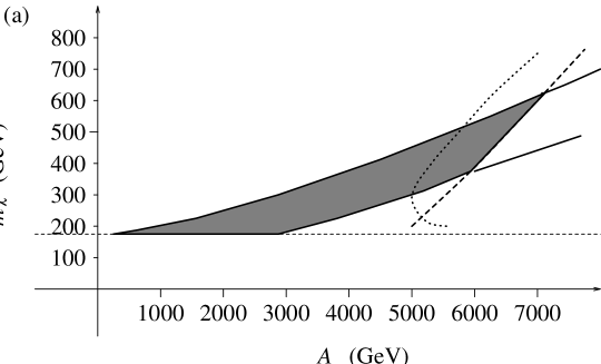
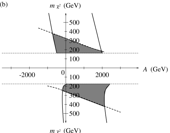
Figure 4: The region of parameters for the squared mass of scalar-quarks to be positive, for (a) $M_{2}+\mu>0$ and (b) $M_{2}-|\mu|<0$. The boundary of vanishing mass of u-type-scalar-quark is represented by solid lines, and that of d-type by dashed lines. In the case (a), allowed region for $m=100$ GeV, $\mu<0$, and $\tan\beta=10$ is denoted by shaded area. For $\tan\beta=100$, the allowed region is the right of dotted line bounded by two solid lines. In the case (b), allowed region for $\mu>0$ is shown in the upper half plane and that for $\mu<0$ in the lower half. Allowed region for $m=100$ GeV and $\tan\beta=10$ is denoted by shaded area.

The presence of the off-diagonal elements of $A$ generally helps to give a larger contribution to EDM. As shown in Fig. 3, the contribution of the chargino diagram to the EDM in fact increases and becomes of the order of $10^{-27}\sim 10^{-29}\ e\cdot\rm{cm}$. In Fig. 3, we have chosen $\tan\beta=10$ and $m_{\chi^{1}}=50$ GeV. One should note that EDM is approximately proportional to $\tan\beta$ for $\tan\beta>5$. In order to see the allowed parameter region, we have plotted in Fig. 4 the region of positive squared masses for scalar-quarks. The allowed parameter regions differ depending on $M_{2}>|\mu|$ (Fig. 4a) or $M_{2}<|\mu|$ (Fig. 4b).

Since d-type-scalar-quarks instead of u-type-scalar-quarks are involved in the loop diagram, we find that the EDM $d_{u}$ of u-quarks is smaller than that of d-quarks and is of the order of $10^{-33}\sim 10^{-35}\>e\cdot$cm.

Next let us examine the gluino contributions to the neutron EDM which is shown in Fig. 2,

$$d_{d}=\frac{e}{16\pi^{2}}g_{3}^{\>2}\frac{4}{3}\frac{1}{M_{3}}{\rm Im}\!\left(G\!\left(\frac{M_{\tilde{d}}^{\prime 2}}{M_{3}^{\>2}}\right)_{\rm RL}\right)_{11},$$ (3.14)

where $g_{3}$ and $M_{3}$ are the strong interaction coupling constant and the mass of the gluino respectively and

$$G(x)\equiv\frac{1}{3(1-x)^{3}}(1-x^{2}+2x\log x).$$ (3.15)

Diagonalizing explicitly the d-type-scalar-quark mass matrix, we find that the EDM $d_{d}$ of the down quark have contributions from this gluino diagram of the order of $10^{-34}\sim 10^{-35}\>e\cdot$cm. The complex phases in off-diagonal elements of $A$ terms are the major source of this contribution.

In the $SU(6)$ quark model, the neutron EDM is given in terms of the single quark EDM as

$$d_{n}={4\over 3}d_{d}-{1\over 3}d_{u}.$$ (3.16)

From the above results, we find that the neutron EDM from the single quark EDM is of the order of $10^{-27}\sim 10^{-29}\>e\cdot$cm for $\tan\beta=10$. The chargino diagram of Fig. 2 is the dominant contribution, since $A$ terms have off-diagonal elements. Although gluino diagrams can also contribute to EDM, its contribution is smaller than that of chargino, since complex phases are almost canceled if one takes the (1,1) component in generation indices.

The contribution of chargino diagram in Fig. 2 was also examined in ref. [10] with somewhat different values of parameters and a result of the order of $10^{-30}\>e\cdot$cm for the EDM of neutron was reported. We have taken account of the evolution of gaugino masses in our renormalization group analysis. This may be a reason for the fact that we have obtained a larger value for the neutron EDM in comparison to ref. [10].

4. Effects of the transition electric dipole moment

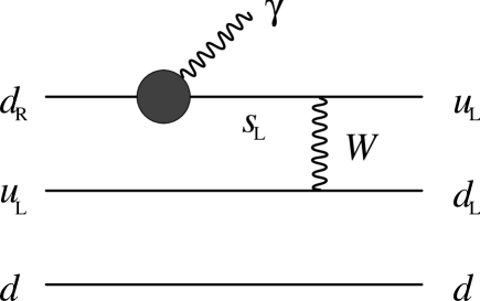
Figure 5: Contribution to the neutron EDM from the TEDM. The diagrams like Fig. 1 or Fig. 2 are inserted in the blob.

Figure 6: For the case $\det M_{\chi}>0$, TEDM ($d\rightarrow s\gamma$) is plotted as a function of the mass $m_{\chi^{2}}$ of the heavier chargino for various values of $A$ in the case (a) $M_{2}+\mu>0$ and (b) $M_{2}+\mu<0$. We have chosen parameters: universal scalar mass $m=100$ GeV, $\tan\beta=10$, and the mass of the light chargino $m_{\chi^{1}}=50$ GeV.

It has been shown that the neutron EDM is also induced in the nonsupersymmetric minimal standard model through the transition electric dipole moment (TEDM) of quarks within the baryon as illustrated in Fig. 6 [15, 16, 17]. In this section, we examine the TEDM, $d\rightarrow s+\gamma$, in the MSSM and calculate the neutron EDM based on their method. The matrix element of the electromagnetic current $j^{\mu}$ between single particle states of different Dirac particles can be written as follows,

$$\langle\mbox{\boldmath$p$}_{f},s_{f}|j^{\mu}(0)|\mbox{\boldmath$p$}_{i},s_{i}\rangle = \bar{u}_{f}(\mbox{\boldmath$p$}_{f},s_{f})\left[i\sigma^{\mu\nu}q_{\nu}\frac{F_{2}(q^{2})}{m_{f}+m_{i}}+\gamma_{5}\sigma^{\mu\nu}q_{\nu}\frac{F_{3}(q^{2})}{m_{f}+m_{i}}\right.$$

$$\qquad\qquad\quad+\{q^{2}\gamma^{\mu}-(m_{f}-m_{i})q^{\mu}\}F_{4}(q^{2})$$

$$\qquad\qquad\quad+\left.\left(\frac{q^{2}}{m_{f}+m_{i}}\gamma^{\mu}-q^{\mu}\right)\gamma_{5}F_{A}(q^{2})\right]u_{i}(\mbox{\boldmath$p$}_{i},s_{i}),$$

where $m_{i}$ and $m_{f}$ are initial and final Dirac fermion masses respectively. The dominant contribution to EDM comes from $F_{3}$ term as that of single quark case when the mass difference $|m_{f}-m_{i}|$ is small enough compared to the other relevant masses. In our particular case, the operator relevant to the TEDM can be written as

$$\kappa^{sd}\bar{s}(p_{s})i\sigma_{\mu\nu}(p_{s}-p_{d})^{\nu}\gamma_{5}d(p_{d}),$$ (4.2)

where

$$i\kappa^{sd}\approx\frac{F_{3}(0)}{m_{s}+m_{d}}.$$ (4.3)

Im $\kappa^{sd}$ is just the TEDM.

The TEDM in the nonsupersymmetric minimal standard model has already been calculated under the assumption that $m_{t}\ll M_{W}$ [15, 16]. Recently it is more and more certain experimentally that the top quark mass is very large [12]. Therefore we must redo the calculation in the nonsupersymmetric case by taking into account of the large top quark mass. Assuming $m_{d}$ and $m_{s}$ to be small in comparison with the masses of the internal lines of the loop diagram, we have the following contribution to the TEDM of $d\rightarrow s+\gamma$,

$$\kappa^{sd}=\frac{G_{F}}{\sqrt{2}}\frac{e}{(4\pi)^{2}}K_{ts}^{*}K_{td}(m_{d}-m_{s})\>f\!\left(\frac{m_{t}^{2}}{M_{W}^{\ 2}}\right),$$ (4.4)

where [20]

$$f(x)\equiv\frac{x}{6(x-1)^{4}}(-8x^{3}+3x^{2}+12x-7+6x(3x-2)\log x).$$ (4.5)

From the above equation, we obtain that the standard model gives $2\cdot 10^{-26}\>e\cdot$cm for the TEDM using the Cabibbo-Kobayashi-Maskawa matrix (A.35) – (A.37). Since the hadronic effects to convert the TEDM to the neutron EDM give a factor of $10^{-7}$ [16], the contribution from the TEDM in the standard model to the neutron EDM becomes of the order of $10^{-33}\>e\cdot$cm.

Next let us consider the TEDM of quarks in the MSSM. Similarly to the quark EDM, the chargino and gluino diagrams are most important. Since the bound state effects should be the same for supersymmetric and nonsupersymmetric models, we shall calculate these diagrams for the quark TEDM and compare them with those of the standard model.

In order to obtain the TEDM, we have only to replace $d_{L}$ by $s_{L}$ in the analysis in the previous section. Similarly to the diagram in Fig. 2, for instance, the chargino contribution is obtained from Eq. (3.4) as

$${\rm Im}\>\kappa^{sd}=\frac{e}{16\pi^{2}}(\tan\beta+\cot\beta)\frac{2}{v^{2}}m_{d}\,{\rm Im}\!\left[\mbox{\boldmath$K$}^{\dagger}\left\{F\!\left(\frac{M_{\tilde{u}}^{\prime 2}}{M_{\chi}^{\dagger}M_{\chi}}\right)_{\rm LR}\frac{1}{M_{\chi}}\right\}_{\rm hh}\mbox{\boldmath$m$}_{u}\mbox{\boldmath$K$}\right]_{12}.$$ (4.6)

Let us note that the element we are interested in is not (2,1) but (1,2) for the LR block of the scalar-quark mass matrix, since the Higgsino coupling changes chirality such as $\tilde{u}^{i}_{R}\rightarrow s_{L}$. By the same token, the gluino diagram for the quark TEDM corresponding to the diagram in Fig. 2 is obtained as

$${\rm Im}\>\kappa^{sd}=\frac{e}{16\pi^{2}}g_{3}^{\>2}\frac{4}{3}\frac{1}{M_{3}}{\rm Im}\!\left(G\!\left(\frac{M_{\tilde{d}}^{\prime 2}}{M_{3}^{\>2}}\right)_{\rm RL}\right)_{12}.$$ (4.7)

In this case, we take the (1,2) element for the RL block because gauge couplings do not change chirality.

We obtain the TEDM of the order of $10^{-25}\sim 10^{-27}\>e\cdot$cm for the chargino contribution as shown in Fig. 6 and $10^{-28}\sim 10^{-30}\>e\cdot$cm for the gluino one. Thus we find that the TEDM in the MSSM is of the same order of magnitude as that in the nonsupersymmetric standard model. By combining our results with the hadronic matrix elements estimated already in the nonsupersymmetric case, we find that the resulting neutron EDM becomes of the order of $10^{-32}\sim 10^{-34}\>e\cdot$cm.

Let us also consider the effects of other diagrams in the supersymmetric model. Besides the diagram which can be considered as the quark TEDM, there are diagrams where two or more quarks within the neutron exchange the SUSY particles. The R-parity conservation in the MSSM dictates that such diagrams must be box diagrams where all of the internal particles are SUSY ones. So the intermediate states at the hadronic level are of the order of mass scale of the SUSY particles which are much heavier than those in the diagrams that we have considered. Therefore the resulting neutron EDM is expected to be highly suppressed.

Apart from the TEDM that we have considered in Fig. 6, another proposal for an effect involving many quarks was made in ref. [17]. They considered the so-called penguin diagrams for the TEDM of quarks. They found that the conversion factor from TEDM to the neutron EDM is $10^{-4}$ instead of $10^{-7}$ due to a large QCD enhancement. Therefore this diagram gives the neutron EDM of the order of $10^{-30}\>e\cdot$cm which is the largest contribution in the nonsupersymmetric standard model. Since the enhancement due to the QCD corrections is the same order of magnitude in the MSSM as in the nonsupersymmetric standard model, we obtain that the neutron EDM is of the order of $10^{-29}\sim 10^{-31}\>e\cdot$cm. Moreover we find from Fig. 6 that the TEDM is of the same order of magnitude even for small values of $A$ such as $A<1$ TeV, whereas the single quark EDM becomes very small as shown in Fig. 3. Therefore the penguin diagram with TEDM is more important than a single quark EDM for smaller values of $A$ ($A\stackrel{{\scriptstyle<}}{{\sim}}1$ TeV).

One of the authors (N.S.) thanks to Y. Okada, T. Goto and J. Hisano for a useful discussion on supersymmetric models and flavor-changing neutral currents. This work is supported in part by Grant-in-Aid for Scientific Research (T.I. and Y.M.) and (No.05640334) (N.S.), and Grant-in-Aid for Scientific Research for Priority Areas (No.06221222) (N.S.) from the Ministry of Education, Science and Culture.

A Renormalization Group Equations

We define the scaling variable $t$ using the GUT scale $M_{GUT}$ and the relevant momentum $Q$ as

$$t\equiv\log\frac{M_{GUT}^{\ 2}}{Q^{2}}.$$ (A.1)

A tilde over couplings denotes a division by a factor $4\pi$, namely $\tilde{\alpha}\equiv\alpha/(4\pi)$. The renormalization group equations for the gauge couplings and gaugino masses $M_{i}$ are given as follows [21]:

$$\dot{\tilde{\alpha}}_{i} = -b_{i}\tilde{\alpha}_{i}^{\ 2},$$ (A.2)

$$\dot{M}_{i} = -b_{i}\tilde{\alpha}_{i}M_{i},$$ (A.3)

where

$$b_{1}=\frac{33}{5}, b_{2}=1, b_{3}=-3,$$ (A.4)

and we denote derivative by $t$ with a dot. The solutions are given as follows:

$$\tilde{\alpha}_{i}(t)=\frac{\tilde{\alpha}_{i}(t_{0})}{1+b_{i}(t-t_{0})\tilde{\alpha}_{i}(t_{0})}=\frac{\tilde{\alpha}_{G}}{1+b_{i}t\tilde{\alpha}_{G}},$$ (A.5)

$$M_{i}(t)=\frac{M_{i}(t_{0})}{1+b_{i}(t-t_{0})\tilde{\alpha}_{i}(t_{0})}=\frac{\tilde{\alpha}_{i}(t)}{\tilde{\alpha}_{i}(t_{0})}M_{i}(t_{0})=\frac{M}{\tilde{\alpha}_{G}}\tilde{\alpha}_{i}(t),$$ (A.6)

where we assume the gauge coupling unification and the universal gaugino mass at the GUT scale:

$$\alpha_{1}(0)=\alpha_{2}(0)=\alpha_{3}(0)=\alpha_{G},$$ (A.7)

$$M_{1}(0)=M_{2}(0)=M_{3}(0)=M.$$ (A.8)

The renormalization group equations for Yukawa couplings are written as follows [21]:

$$2\dot{\widetilde{\mbox{\boldmath$Y$}}}_{u} = \left(\frac{13}{15}\tilde{\alpha}_{1}+3\tilde{\alpha}_{2}+\frac{16}{3}\tilde{\alpha}_{3}\right)\widetilde{\mbox{\boldmath$Y$}}_{u}-\left[3\widetilde{\mbox{\boldmath$Y$}}_{u}\widetilde{\mbox{\boldmath$Y$}}_{u}^{\dagger}\widetilde{\mbox{\boldmath$Y$}}_{u}+3{\rm Tr}\left(\widetilde{\mbox{\boldmath$Y$}}_{u}\widetilde{\mbox{\boldmath$Y$}}_{u}^{\dagger}\right)\widetilde{\mbox{\boldmath$Y$}}_{u}\right]$$ (A.9)

$$-\widetilde{\mbox{\boldmath$Y$}}_{u}\widetilde{\mbox{\boldmath$Y$}}_{d}^{\dagger}\widetilde{\mbox{\boldmath$Y$}}_{d},$$

$$2\dot{\widetilde{\mbox{\boldmath$Y$}}}_{d} = \left(\frac{7}{15}\tilde{\alpha}_{1}+3\tilde{\alpha}_{2}+\frac{16}{3}\tilde{\alpha}_{3}\right)\widetilde{\mbox{\boldmath$Y$}}_{d}-\left[3\widetilde{\mbox{\boldmath$Y$}}_{d}\widetilde{\mbox{\boldmath$Y$}}_{d}^{\dagger}\widetilde{\mbox{\boldmath$Y$}}_{d}+3{\rm Tr}\left(\widetilde{\mbox{\boldmath$Y$}}_{d}\widetilde{\mbox{\boldmath$Y$}}_{d}^{\dagger}\right)\widetilde{\mbox{\boldmath$Y$}}_{d}\right]$$ (A.10)

$$-\widetilde{\mbox{\boldmath$Y$}}_{d}\widetilde{\mbox{\boldmath$Y$}}_{u}^{\dagger}\widetilde{\mbox{\boldmath$Y$}}_{u}-{\rm Tr}\left(\widetilde{\mbox{\boldmath$Y$}}_{e}\widetilde{\mbox{\boldmath$Y$}}_{e}^{\dagger}\right)\widetilde{\mbox{\boldmath$Y$}}_{d},$$

$$2\dot{\widetilde{\mbox{\boldmath$Y$}}}_{e} = \left(\frac{9}{5}\tilde{\alpha}_{1}+3\tilde{\alpha}_{2}\right)\widetilde{\mbox{\boldmath$Y$}}_{e}-\left[3\widetilde{\mbox{\boldmath$Y$}}_{e}\widetilde{\mbox{\boldmath$Y$}}_{e}^{\dagger}\widetilde{\mbox{\boldmath$Y$}}_{e}+{\rm Tr}\left(\widetilde{\mbox{\boldmath$Y$}}_{e}\widetilde{\mbox{\boldmath$Y$}}_{e}^{\dagger}\right)\widetilde{\mbox{\boldmath$Y$}}_{e}\right]$$ (A.11)

$$-3{\rm Tr}\left(\widetilde{\mbox{\boldmath$Y$}}_{d}\widetilde{\mbox{\boldmath$Y$}}_{d}^{\dagger}\right)\widetilde{\mbox{\boldmath$Y$}}_{e}.$$

We now define hermitian matrices $\tilde{\mbox{\boldmath$\alpha$}}_{f}$ ($f=u,d,e$),

$$\tilde{\mbox{\boldmath$\alpha$}}_{f}\equiv\widetilde{\mbox{\boldmath$Y$}}_{f}^{\dagger}\widetilde{\mbox{\boldmath$Y$}}_{f}.$$ (A.12)

The renormalization group equations for $\tilde{\mbox{\boldmath$\alpha$}}_{f}$ are given as follows:

$$2\dot{\tilde{\mbox{\boldmath$\alpha$}}}_{u} = 2\left(\frac{13}{15}\tilde{\alpha}_{1}+3\tilde{\alpha}_{2}+\frac{16}{3}\tilde{\alpha}_{3}\right)\tilde{\mbox{\boldmath$\alpha$}}_{u}-2\left[3\tilde{\mbox{\boldmath$\alpha$}}_{u}^{\ 2}+3{\rm Tr}\left(\tilde{\mbox{\boldmath$\alpha$}}_{u}\right)\tilde{\mbox{\boldmath$\alpha$}}_{u}\right]$$ (A.13)

$$-\tilde{\mbox{\boldmath$\alpha$}}_{d}\tilde{\mbox{\boldmath$\alpha$}}_{u}-\tilde{\mbox{\boldmath$\alpha$}}_{u}\tilde{\mbox{\boldmath$\alpha$}}_{d},$$

$$2\dot{\tilde{\mbox{\boldmath$\alpha$}}}_{d} = 2\left(\frac{7}{15}\tilde{\alpha}_{1}+3\tilde{\alpha}_{2}+\frac{16}{3}\tilde{\alpha}_{3}\right)\tilde{\mbox{\boldmath$\alpha$}}_{d}-2\left[3\tilde{\mbox{\boldmath$\alpha$}}_{d}^{\ 2}+3{\rm Tr}\left(\tilde{\mbox{\boldmath$\alpha$}}_{d}\right)\tilde{\mbox{\boldmath$\alpha$}}_{d}\right]-2{\rm Tr}\left(\tilde{\mbox{\boldmath$\alpha$}}_{e}\right)\tilde{\mbox{\boldmath$\alpha$}}_{d}$$ (A.14)

$$-\tilde{\mbox{\boldmath$\alpha$}}_{u}\tilde{\mbox{\boldmath$\alpha$}}_{d}-\tilde{\mbox{\boldmath$\alpha$}}_{d}\tilde{\mbox{\boldmath$\alpha$}}_{u},$$

$$\dot{\tilde{\mbox{\boldmath$\alpha$}}}_{e} = \left(\frac{9}{5}\tilde{\alpha}_{1}+3\tilde{\alpha}_{2}\right)\tilde{\mbox{\boldmath$\alpha$}}_{e}-\left[3\tilde{\mbox{\boldmath$\alpha$}}_{e}^{\ 2}+{\rm Tr}\left(\tilde{\mbox{\boldmath$\alpha$}}_{e}\right)\tilde{\mbox{\boldmath$\alpha$}}_{e}\right]-3{\rm Tr}\left(\tilde{\mbox{\boldmath$\alpha$}}_{d}\right)\tilde{\mbox{\boldmath$\alpha$}}_{e}.$$ (A.15)

The renormalization group equations for $A$’s can be written as follows [21, 10]:

$$2\dot{\mbox{\boldmath$A$}}_{u} = -2\left(\frac{13}{15}\tilde{\alpha}_{1}M_{1}+3\tilde{\alpha}_{2}M_{2}+\frac{16}{3}\tilde{\alpha}_{3}M_{3}\right){\bf 1}-2{\rm Tr}\left(3\mbox{\boldmath$A$}_{u}\tilde{\mbox{\boldmath$\alpha$}}_{u}\right){\bf 1}$$ (A.16)

$$-5\tilde{\mbox{\boldmath$\alpha$}}_{u}\mbox{\boldmath$A$}_{u}-\mbox{\boldmath$A$}_{u}\tilde{\mbox{\boldmath$\alpha$}}_{u}-\tilde{\mbox{\boldmath$\alpha$}}_{d}\mbox{\boldmath$A$}_{u}+\mbox{\boldmath$A$}_{u}\tilde{\mbox{\boldmath$\alpha$}}_{d}-2\mbox{\boldmath$A$}_{d}\tilde{\mbox{\boldmath$\alpha$}}_{d},$$

$$2\dot{\mbox{\boldmath$A$}}_{d} = -2\left(\frac{7}{15}\tilde{\alpha}_{1}M_{1}+3\tilde{\alpha}_{2}M_{2}+\frac{16}{3}\tilde{\alpha}_{3}M_{3}\right){\bf 1}-2{\rm Tr}\left(\mbox{\boldmath$A$}_{e}\tilde{\mbox{\boldmath$\alpha$}}_{e}+3\mbox{\boldmath$A$}_{d}\tilde{\mbox{\boldmath$\alpha$}}_{d}\right){\bf 1}$$ (A.17)

$$-5\tilde{\mbox{\boldmath$\alpha$}}_{d}\mbox{\boldmath$A$}_{d}-\mbox{\boldmath$A$}_{d}\tilde{\mbox{\boldmath$\alpha$}}_{d}-\tilde{\mbox{\boldmath$\alpha$}}_{u}\mbox{\boldmath$A$}_{d}+\mbox{\boldmath$A$}_{d}\tilde{\mbox{\boldmath$\alpha$}}_{u}-2\mbox{\boldmath$A$}_{u}\tilde{\mbox{\boldmath$\alpha$}}_{u},$$

$$\dot{\mbox{\boldmath$A$}}_{e} = -2\left(\frac{9}{5}\tilde{\alpha}_{1}M_{1}+3\tilde{\alpha}_{2}M_{2}\right){\bf 1}-2{\rm Tr}\left(\mbox{\boldmath$A$}_{e}\tilde{\mbox{\boldmath$\alpha$}}_{e}+3\mbox{\boldmath$A$}_{d}\tilde{\mbox{\boldmath$\alpha$}}_{d}\right){\bf 1}$$ (A.18)

$$-5\tilde{\mbox{\boldmath$\alpha$}}_{e}\mbox{\boldmath$A$}_{e}-\mbox{\boldmath$A$}_{e}\tilde{\mbox{\boldmath$\alpha$}}_{e}.$$

Next we consider the renormalization group equations in the super KM basis, i.e., we rotate Yukawa couplings $\widetilde{\mbox{\boldmath$Y$}}_{f}$ by the same amount as $\mbox{\boldmath$M$}_{f}$ in Eqs. (2.44) and (2.45), and $\mbox{\boldmath$A$}_{f}$ and $\tilde{\mbox{\boldmath$\alpha$}}_{f}$ by the same amount as $\mbox{\boldmath$A$}_{f}$ in Eq. (2.47). In this basis the renormalization group equations are given as follows:

$$2\dot{\tilde{\mbox{\boldmath$\alpha$}}}_{u} = 2\left(\frac{13}{15}\tilde{\alpha}_{1}+3\tilde{\alpha}_{2}+\frac{16}{3}\tilde{\alpha}_{3}\right)\tilde{\mbox{\boldmath$\alpha$}}_{u}-2\left[3\tilde{\mbox{\boldmath$\alpha$}}_{u}^{\ 2}+3{\rm Tr}\left(\tilde{\mbox{\boldmath$\alpha$}}_{u}\right)\tilde{\mbox{\boldmath$\alpha$}}_{u}\right]$$ (A.19)

$$-\mbox{\boldmath$K$}\tilde{\mbox{\boldmath$\alpha$}}_{d}\mbox{\boldmath$K$}^{\dagger}\tilde{\mbox{\boldmath$\alpha$}}_{u}-\tilde{\mbox{\boldmath$\alpha$}}_{u}\mbox{\boldmath$K$}\tilde{\mbox{\boldmath$\alpha$}}_{d}\mbox{\boldmath$K$}^{\dagger},$$

$$2\dot{\tilde{\mbox{\boldmath$\alpha$}}}_{d} = 2\left(\frac{7}{15}\tilde{\alpha}_{1}+3\tilde{\alpha}_{2}+\frac{16}{3}\tilde{\alpha}_{3}\right)\tilde{\mbox{\boldmath$\alpha$}}_{d}-2\left[3\tilde{\mbox{\boldmath$\alpha$}}_{d}^{\ 2}+3{\rm Tr}\left(\tilde{\mbox{\boldmath$\alpha$}}_{d}\right)\tilde{\mbox{\boldmath$\alpha$}}_{d}\right]-2{\rm Tr}\left(\tilde{\mbox{\boldmath$\alpha$}}_{e}\right)\tilde{\mbox{\boldmath$\alpha$}}_{d}$$ (A.20)

$$-\mbox{\boldmath$K$}^{\dagger}\tilde{\mbox{\boldmath$\alpha$}}_{u}\mbox{\boldmath$K$}\tilde{\mbox{\boldmath$\alpha$}}_{d}-\tilde{\mbox{\boldmath$\alpha$}}_{d}\mbox{\boldmath$K$}^{\dagger}\tilde{\mbox{\boldmath$\alpha$}}_{u}\mbox{\boldmath$K$},$$

$$\dot{\tilde{\mbox{\boldmath$\alpha$}}}_{e} = \left(\frac{9}{5}\tilde{\alpha}_{1}+3\tilde{\alpha}_{2}\right)\tilde{\mbox{\boldmath$\alpha$}}_{e}-\left[3\tilde{\mbox{\boldmath$\alpha$}}_{e}^{\ 2}+{\rm Tr}\left(\tilde{\mbox{\boldmath$\alpha$}}_{e}\right)\tilde{\mbox{\boldmath$\alpha$}}_{e}\right]-3{\rm Tr}\left(\tilde{\mbox{\boldmath$\alpha$}}_{d}\right)\tilde{\mbox{\boldmath$\alpha$}}_{e},$$ (A.21)

$$2\dot{\mbox{\boldmath$A$}}_{u} = -2\left(\frac{13}{15}\tilde{\alpha}_{1}M_{1}+3\tilde{\alpha}_{2}M_{2}+\frac{16}{3}\tilde{\alpha}_{3}M_{3}\right){\bf 1}-2{\rm Tr}\left(3\mbox{\boldmath$A$}_{u}\tilde{\mbox{\boldmath$\alpha$}}_{u}\right){\bf 1}$$ (A.22)

$$\!\!\!\!\!\!-5\tilde{\mbox{\boldmath$\alpha$}}_{u}\mbox{\boldmath$A$}_{u}-\mbox{\boldmath$A$}_{u}\tilde{\mbox{\boldmath$\alpha$}}_{u}-\mbox{\boldmath$K$}\tilde{\mbox{\boldmath$\alpha$}}_{d}\mbox{\boldmath$K$}^{\dagger}\mbox{\boldmath$A$}_{u}+\mbox{\boldmath$A$}_{u}\mbox{\boldmath$K$}\tilde{\mbox{\boldmath$\alpha$}}_{d}\mbox{\boldmath$K$}^{\dagger}-2\mbox{\boldmath$K$}\mbox{\boldmath$A$}_{d}\tilde{\mbox{\boldmath$\alpha$}}_{d}\mbox{\boldmath$K$}^{\dagger},$$

$$2\dot{\mbox{\boldmath$A$}}_{d} = -2\left(\frac{7}{15}\tilde{\alpha}_{1}M_{1}+3\tilde{\alpha}_{2}M_{2}+\frac{16}{3}\tilde{\alpha}_{3}M_{3}\right){\bf 1}-2{\rm Tr}\left(\mbox{\boldmath$A$}_{e}\tilde{\mbox{\boldmath$\alpha$}}_{e}+3\mbox{\boldmath$A$}_{d}\tilde{\mbox{\boldmath$\alpha$}}_{d}\right){\bf 1}$$ (A.23)

$$\!\!\!\!\!\!-5\tilde{\mbox{\boldmath$\alpha$}}_{d}\mbox{\boldmath$A$}_{d}-\mbox{\boldmath$A$}_{d}\tilde{\mbox{\boldmath$\alpha$}}_{d}-\mbox{\boldmath$K$}^{\dagger}\tilde{\mbox{\boldmath$\alpha$}}_{u}\mbox{\boldmath$K$}\mbox{\boldmath$A$}_{d}+\mbox{\boldmath$A$}_{d}\mbox{\boldmath$K$}^{\dagger}\tilde{\mbox{\boldmath$\alpha$}}_{u}\mbox{\boldmath$K$}-2\mbox{\boldmath$K$}^{\dagger}\mbox{\boldmath$A$}_{u}\tilde{\mbox{\boldmath$\alpha$}}_{u}\mbox{\boldmath$K$},$$

$$\dot{\mbox{\boldmath$A$}_{e}} = -2\left(\frac{9}{5}\tilde{\alpha}_{1}M_{1}+3\tilde{\alpha}_{2}M_{2}\right){\bf 1}-2{\rm Tr}\left(\mbox{\boldmath$A$}_{e}\tilde{\mbox{\boldmath$\alpha$}}_{e}+3\mbox{\boldmath$A$}_{d}\tilde{\mbox{\boldmath$\alpha$}}_{d}\right){\bf 1}$$ (A.24)

$$-5\tilde{\mbox{\boldmath$\alpha$}}_{e}\mbox{\boldmath$A$}_{e}-\mbox{\boldmath$A$}_{e}\tilde{\mbox{\boldmath$\alpha$}}_{e}.$$

In Eqs. (A.19) – (A.21), we give the initial conditions for $\tilde{\mbox{\boldmath$\alpha$}}_{f}$ ($f=u,d,e$) at the scale of $Z^{0}$ boson mass $M_{Z}$ which are obtained from the quark and lepton masses, i.e.,

$$\tilde{\mbox{\boldmath$\alpha$}}_{u} = \left(\frac{\sqrt{2}}{4\pi v\sin\beta}\right)^{2}\mbox{\boldmath$m$}_{u}^{\ 2},$$ (A.25)

$$\tilde{\mbox{\boldmath$\alpha$}}_{d} = \left(\frac{\sqrt{2}}{4\pi v\cos\beta}\right)^{2}\mbox{\boldmath$m$}_{d}^{\ 2},$$ (A.26)

$$\tilde{\mbox{\boldmath$\alpha$}}_{e} = \left(\frac{\sqrt{2}}{4\pi v\cos\beta}\right)^{2}\mbox{\boldmath$m$}_{e}^{\ 2}$$ (A.27)

at the scale $M_{Z}$ and we obtain solutions for $\tilde{\mbox{\boldmath$\alpha$}}_{f}$. The $\tilde{\mbox{\boldmath$\alpha$}}_{f}$ are diagonal at the initial condition and then $\tilde{\mbox{\boldmath$\alpha$}}_{e}$ is diagonal at all the scale but $\tilde{\mbox{\boldmath$\alpha$}}_{u}$ and $\tilde{\mbox{\boldmath$\alpha$}}_{d}$ are not diagonal at the higher scale.

In Eqs. (A.22) – (A.24), we give the initial conditions for $\mbox{\boldmath$A$}_{f}$ ($f=u,d,e$) at the GUT scale $M_{GUT}$ which are universal, i.e.,

$$\mbox{\boldmath$A$}_{u}(0)=\mbox{\boldmath$A$}_{d}(0)=\mbox{\boldmath$A$}_{e}(0)=A{\bf 1}.$$ (A.28)

The $\mbox{\boldmath$A$}_{f}$ are diagonal at the initial condition. Then $\mbox{\boldmath$A$}_{e}$ is diagonal at all the scale, but $\mbox{\boldmath$A$}_{u}$ and $\mbox{\boldmath$A$}_{d}$ are not diagonal at the lower scale. It is convenient to separate $\mbox{\boldmath$A$}_{f}$ into two parts.

$$\mbox{\boldmath$A$}_{f}=\mbox{\boldmath$A$}_{Lf}+\mbox{\boldmath$A$}_{Mf},$$ (A.29)

where $f=u,d,e$. The same renormalization group equations (A.22) – (A.24) as $\mbox{\boldmath$A$}_{f}$ are valid for $\mbox{\boldmath$A$}_{Mf}$ which are proportional to the universal gaugino mass $M$. Their initial conditions at the GUT scale are

$$\mbox{\boldmath$A$}_{Mu}(0)=\mbox{\boldmath$A$}_{Md}(0)=\mbox{\boldmath$A$}_{Me}(0)=0.$$ (A.30)

By deleting gaugino masses from Eqs. (A.22) – (A.24), we obtain linear equations for $\mbox{\boldmath$A$}_{Lf}$:

$$2\dot{\mbox{\boldmath$A$}}_{Lu} = -2{\rm Tr}\left(3\mbox{\boldmath$A$}_{Lu}\tilde{\mbox{\boldmath$\alpha$}}_{u}\right){\bf 1}-5\tilde{\mbox{\boldmath$\alpha$}}_{u}\mbox{\boldmath$A$}_{Lu}-\mbox{\boldmath$A$}_{Lu}\tilde{\mbox{\boldmath$\alpha$}}_{u}$$ (A.31)

$$-\mbox{\boldmath$K$}\tilde{\mbox{\boldmath$\alpha$}}_{d}\mbox{\boldmath$K$}^{\dagger}\mbox{\boldmath$A$}_{Lu}+\mbox{\boldmath$A$}_{Lu}\mbox{\boldmath$K$}\tilde{\mbox{\boldmath$\alpha$}}_{d}\mbox{\boldmath$K$}^{\dagger}-2\mbox{\boldmath$K$}\mbox{\boldmath$A$}_{Ld}\tilde{\mbox{\boldmath$\alpha$}}_{d}\mbox{\boldmath$K$}^{\dagger},$$

$$2\dot{\mbox{\boldmath$A$}}_{Ld} = -2{\rm Tr}\left(\mbox{\boldmath$A$}_{Le}\tilde{\mbox{\boldmath$\alpha$}}_{e}+3\mbox{\boldmath$A$}_{Ld}\tilde{\mbox{\boldmath$\alpha$}}_{d}\right){\bf 1}-5\tilde{\mbox{\boldmath$\alpha$}}_{d}\mbox{\boldmath$A$}_{Ld}-\mbox{\boldmath$A$}_{Ld}\tilde{\mbox{\boldmath$\alpha$}}_{d}$$ (A.32)

$$-\mbox{\boldmath$K$}^{\dagger}\tilde{\mbox{\boldmath$\alpha$}}_{u}\mbox{\boldmath$K$}\mbox{\boldmath$A$}_{Ld}+\mbox{\boldmath$A$}_{Ld}\mbox{\boldmath$K$}^{\dagger}\tilde{\mbox{\boldmath$\alpha$}}_{u}\mbox{\boldmath$K$}-2\mbox{\boldmath$K$}^{\dagger}\mbox{\boldmath$A$}_{Lu}\tilde{\mbox{\boldmath$\alpha$}}_{u}\mbox{\boldmath$K$},$$

$$\dot{\mbox{\boldmath$A$}}_{Le} = -2{\rm Tr}\left(\mbox{\boldmath$A$}_{Le}\tilde{\mbox{\boldmath$\alpha$}}_{e}+3\mbox{\boldmath$A$}_{Ld}\tilde{\mbox{\boldmath$\alpha$}}_{d}\right){\bf 1}-5\tilde{\mbox{\boldmath$\alpha$}}_{e}\mbox{\boldmath$A$}_{Le}-\mbox{\boldmath$A$}_{Le}\tilde{\mbox{\boldmath$\alpha$}}_{e}.$$ (A.33)

The initial conditions are the same as $\mbox{\boldmath$A$}_{f}$ and are proportional to $A$, i.e.,

$$\mbox{\boldmath$A$}_{Lu}(0)=\mbox{\boldmath$A$}_{Ld}(0)=\mbox{\boldmath$A$}_{Le}(0)=A{\bf 1}.$$ (A.34)

We consider $m_{t}=174$ GeV [12]. The Cabibbo-Kobayashi-Maskawa matrix is parametrized as [22]

$$\mbox{\boldmath$K$}=\left(\!\!\begin{array}[]{ccc}c_{2}c_{3}&c_{2}s_{3}&s_{2}e^{-i\delta}\\ -c_{1}s_{3}-s_{1}s_{2}c_{3}e^{i\delta}&c_{1}c_{3}-s_{1}s_{2}s_{3}e^{i\delta}&s_{1}c_{2}\\ s_{1}s_{3}-c_{1}s_{2}c_{3}e^{i\delta}&-s_{1}c_{3}-c_{1}s_{2}s_{3}e^{i\delta}&c_{1}c_{2}\end{array}\!\!\right),$$ (A.35)

where

$$c_{i}=\cos\theta_{i},\qquad s_{i}=\sin\theta_{i}\qquad(i=1,2,3).$$ (A.36)

We use the following angles from phenomenological analyses [22]

$$\theta_{1}=0.043,\quad\theta_{2}=0.005,\quad\theta_{3}=0.221,\quad\delta=0.86.$$ (A.37)

For $\tan\beta=10$ and $A=1$ GeV, we obtain $A_{Lf}$ at the scale $M_{Z}$ by solving the renormalization group equations:

$$\mbox{\boldmath$A$}_{Lu}=\left(\!\!\begin{array}[]{ccc}0.60&(-5.4+i1.8)\cdot 10^{-6}&(-3.6+i4.2)\cdot 10^{-5}\\ (-5.4-i1.8)\cdot 10^{-6}&0.60&-4.8\cdot 10^{-4}\\ (-3.6-i4.2)\cdot 10^{-5}&-4.8\cdot 10^{-4}&0.19\end{array}\!\!\right),$$ (A.38)

$$\mbox{\boldmath$A$}_{Ld}=\left(\!\!\begin{array}[]{ccc}0.96&(3.7+i2.2)\cdot 10^{-5}&(-8.3-i4.9)\cdot 10^{-4}\\ (3.7-i2.2)\cdot 10^{-5}&0.96&(5.7-i0.1)\cdot 10^{-3}\\ (-8.3+i4.9)\cdot 10^{-4}&(5.7+i0.1)\cdot 10^{-3}&0.79\end{array}\!\!\right),$$ (A.39)

$$\mbox{\boldmath$A$}_{Le}=\left(\!\!\begin{array}[]{ccc}0.96&0&0\\ 0&0.96&0\\ 0&0&0.95\end{array}\!\!\right).$$ (A.40)

For $\tan\beta=10$ and $M=1$ GeV, we obtain $A_{Mf}$ at the scale $M_{Z}$:

$$\mbox{\boldmath$A$}_{Mu}=\left(\!\!\begin{array}[]{ccc}-2.9&(1.1-i0.4)\cdot 10^{-5}&(7.6-i8.9)\cdot 10^{-5}\\ (1.1+i0.4)\cdot 10^{-5}&-2.9&0.0010\\ (7.6+i8.9)\cdot 10^{-5}&0.0010&-2.1\end{array}\!\!\right),$$ (A.41)

$$\mbox{\boldmath$A$}_{Md}=\left(\!\!\begin{array}[]{ccc}-3.7&(-8.0-i4.7)\cdot 10^{-5}&(1.8-i1.1)\cdot 10^{-3}\\ (-8.0+i4.7)\cdot 10^{-5}&-3.7&-0.012\\ (1.8+i1.1)\cdot 10^{-3}&-0.012&-3.3\end{array}\!\!\right),$$ (A.42)

$$\mbox{\boldmath$A$}_{Me}=\left(\!\!\begin{array}[]{ccc}-0.62&0&0\\ 0&-0.62&0\\ 0&0&-0.61\end{array}\!\!\right).$$ (A.43)

Figure captions

• The chargino contribution to the quark EDM involving Higgsino couplings. The arrow on each line stands for the chirality of the particle and the cross for mass insertion.

• The gluino contribution to the quark EDM.

• For the case $\det M_{\chi}>0$, EDM of the down quark is plotted as a function of the mass $m_{\chi^{2}}$ of the heavier chargino for various values of $A$ in the case (a) $M_{2}+\mu>0$ and (b) $M_{2}+\mu<0$. We have chosen parameters: universal scalar-mass $m=100$ GeV, $\tan\beta=10$, and the mass of the light chargino $m_{\chi^{1}}=50$ GeV.

• The region of parameters for the squared mass of scalar-quarks to be positive, for (a) $M_{2}+\mu>0$ and (b) $M_{2}-|\mu|<0$. The boundary of vanishing mass of u-type-scalar-quark is represented by solid lines, and that of d-type by dashed lines. In the case (a), allowed region for $m=100$ GeV, $\mu<0$, and $\tan\beta=10$ is denoted by shaded area. For $\tan\beta=100$, the allowed region is the right of dotted line bounded by two solid lines. In the case (b), allowed region for $\mu>0$ is shown in the upper half plane and that for $\mu<0$ in the lower half. Allowed region for $m=100$ GeV and $\tan\beta=10$ is denoted by shaded area.

• Contribution to the neutron EDM through the TEDM. The diagrams like Fig. 2 or Fig. 2 is inserted in the blob.

• For the case $\det M_{\chi}>0$, TEDM ($d\rightarrow s\gamma$) is plotted as a function of the mass $m_{\chi^{2}}$ of the heavier chargino for various values of $A$ in the case (a) $M_{2}+\mu>0$ and (b) $M_{2}+\mu<0$. We have chosen parameters: universal scalar mass $m=100$ GeV, $\tan\beta=10$, and the mass of the light chargino $m_{\chi^{1}}=50$ GeV.

Figure 1: The chargino contribution to the quark EDM involving Higgsino couplings. The arrow on each line stands for the chirality of the particle and the cross for mass insertion.

Figure 2: The gluino contribution to the quark EDM.

Figure 3: For the case $\det M_{\chi}>0$, EDM of the down quark is plotted as a function of the mass $m_{\chi^{2}}$ of the heavier chargino for various values of $A$ in the case (a) $M_{2}+\mu>0$ and (b) $M_{2}+\mu<0$. We have chosen parameters: universal scalar mass $m=100$ GeV, $\tan\beta=10$, and the mass of the light chargino $m_{\chi^{1}}=50$ GeV.

References

• [1] For a review on supersymmetric models, see for instance, H.P. Nilles, Phys. Rev. C110 (1984) 1; P. Nath, R. Arnowitt, and A. Chamseddine, Applied $N=1$ Supergravity, the ICTP Series in Theoretical Physics, Vol. I (World scientific) 1984; H. Haber and G. Kane, Phys. Rev. C117 (1985) 75; S. Ferrara, Supersymmetry, Vol. I and II (World scientific) 1987.
• [2] S. Dimopoulos and H. Georgi, Nucl. Phys. B193 (1981) 150; N. Sakai, Z. f. Phys. C11 (1981) 153; E. Witten, Nucl. Phys. B188 (1981) 513.
• [3] U. Amaldi, W. de Boer and H. Fürstenau, Phys. Lett. B260 (1991) 447; J. Ellis, S. Kelly and D.V. Nanopoulos, Phys. Lett. B260 (1991) 131.
• [4] A.D. Sakharov, JETP 5 (1967) 24; M. Yoshimura, Phys. Rev. Lett. 41 (1978) 281.
• [5] For a review on electric dipole moments, see for instance, S.M. Barr and W.J. Marciano, Electric dipole moments, in CP violation ed. C. Jarlskog, (1989, World Scientific., Singapore), p. 455.
• [6] Y. Kizukuri and N. Oshimo, Phys. Rev. D45 (1992) 1806; Phys. Rev. D46 (1992) 3025.
• [7] W. Buchmuller and D. Wyler, Phys. Lett. B121 (1983) 321; J. Polchinski and M.B. Wise, Phys. Lett. B125 (1983) 393; F. del Aguila et. al., Phys. Lett. B126 (1983) 71.
• [8] S. Weinberg, Phys. Rev. Lett. 63 (1989) 2333; R. Arnowitt, J.L. Lopez and D.V. Nanopoulos, Phys. Rev. D42 (1990) 2423; R. Arnowitt, M. Duff and K.S. Stelle, Phys. Rev. D43 (1991) 3085.
• [9] P. Nath, R. Arnowitt, and A. Chamseddine, Phys. Rev. Lett. 49 (1982) 970.
• [10] S. Bertolini and F. Vissani, Phys. Lett. B324 (1994) 164.
• [11] T. Goto, T. Nihei, and J. Arafune, 1994, Preprint No. ICRR-317-94-12, hep-ph/9404349.
• [12] CDF collaboration, Phys. Rev. Lett. 73 (1994) 225.
• [13] S. Dimopoulos and L.J. Hall, LBL-36269, hep-ph.9411273; R. Barbieri, L. Hall and A. Strumia, IFUP-TH 72/94, hep-ph.9501334; T. Kobayashi, M. Konmura, D. Suematsu, K. Yamada, and Y. Yamagishi, preprint Kanazawa-94-17.
• [14] T. Hayashi, Y. Koide, M. Matsuda, M. Tanimoto, and S. Wakaizumi, preprint UWThPh-1994-48.
• [15] B.F. Morel, Nucl. Phys. B157 (1979) 23; D.V. Nanopoulos, A. Yildiz, and P. Cox, Phys. Lett. B87 (1979) 53.
• [16] M.B. Gavela, A. Le Yaouanc, L. Oliver, O. Pène, J. C. Raynal and T.N. Pham, Phys. Lett. B109 (1982) 83; E.P. Shabalin, Sov. J. Nucl. Phys. 32 (1980) 228; N. Despande, G. Eilam, and W. Spence, Phys. Lett. B108 (1982) 42.
• [17] M.B. Gavela, A. Le Yaouanc, L. Oliver, O. Pène, J. C. Raynal and T.N. Pham, Phys. Lett. B109 (1982) 215.
• [18] S.P. Martin and P. Ramond, Phys. Rev. D48 (1993) 5365.
• [19] K. Inoue, A. Kakuto, H. Komatsu, and S. Takeshita, Prog. Theor. Phys. 67 (1983) 1889; L. Alvarez-Gaume, J. Polchinski, and M.B. Wise, Nucl. Phys. B221 (1983) 495.
• [20] T. Inami and C. S. Lim, Prog. Theor. Phys. 65 (1981) 297.
• [21] S. Bertolini, F. Borzumati, A. Masiero and G. Ridolfi, Nucl. Phys. B353 (1991) 591.
• [22] Review of Particle Properties, Particle Data Group, Phys. Rev. D45 (1992) 1.