DTP/95/26

March 1995

(Revised May 1995)

Deep Inelastic Electron–Pomeron
Scattering at HERA
T. Gehrmann and W.J. Stirling
Department of Physics, University of Durham
Durham DH1 3LE, England

The idea that the pomeron has partonic structure similar to any other hadron has been given strong support by recent measurements of the diffractive structure function at HERA. We present a detailed theoretical analysis of the diffractive structure function under the assumption that the diffractive cross section can be factorized into a pomeron emission factor and the deep inelastic scattering cross section of the pomeron. We pay particular attention to the kinematic correlations implied by this picture, and suggest the measurement of an angular correlation which should provide a first test of the whole picture. We also present two simple phenomenological models for the quark and gluon structure of the pomeron, which are consistent with various theoretical ideas and which give equally good fits to recent measurements by the H1 collaboration, when combined with the pomeron emission factor of Donnachie and Landshoff. We predict that a large fraction of diffractive deep inelastic events will contain charm, and discuss how improved data will be able to distinguish the models.

1 Introduction

Recent measurements at HERA have indicated that a significant fraction of deep inelastic electron-proton scattering events have a final state with a large rapidity gap between the proton beam direction and the observed final state particles [1, 2]. The lack of any hadronic activity around the proton beam direction and the mismatch between the initial-state and observed final-state energy requires the proton (deflected only by a small angle and therefore outside the rapidity coverage of the detectors) to be in the final state, still carrying a large fraction of its incident momentum. These events with a remnant proton in the final state are classified as diffractive scattering (DS). In analogy to the conventional deep inelastic scattering (DIS) cross section, the differential cross section for DS can be written as

$$\frac{{\rm d}\sigma^{D\!S}}{{\rm d}\alpha_{p}{\rm d}t{\rm d}x{\rm d}Q^{2}}\;=\;\frac{4\pi\alpha^{2}}{xQ^{4}}\;\left\{1-y+\frac{y^{2}}{2[1+R^{D\!S}(x,Q^{2},\alpha_{p},t)]}\right\}\;F_{2}^{D\!S}(x,Q^{2},\alpha_{p},t).$$ (1)

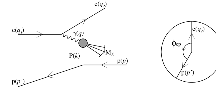
Figure 1: Kinematics of deep inelastic electron-pomeron scattering

The final state configuration of these events suggests that they are caused by a deep inelastic scattering of an uncharged and uncoloured object, which was emitted from the proton beforehand, Fig. 1. From the kinematical distribution of the diffractive events it seems most likely that this object is the pomeron, which so far has only been observed and identified by its $t$-channel trajectory [3] in the full hadron-hadron cross section. The idea that the pomeron has hard partonic constituents was first proposed by Ingelman and Schlein [5], and given strong support by the hadron collider experiments of the UA8 collaboration [6, 7].

If this interpretation is correct, then one would expect that the diffractive cross section could be factorized into a piece corresponding to the emission of an uncharged, colourless pomeron from the proton and a piece corresponding to a hard scattering off the partonic constituents of the pomeron:

$$\frac{{\rm d}\sigma^{D\!S}}{{\rm d}\alpha_{p}{\rm d}t{\rm d}z{\rm d}Q^{2}}\;=\;\frac{4\pi\alpha^{2}}{zQ^{4}}\;\left\{1-y_{P}+\frac{y_{P}^{2}}{2[1+R^{P}(z,Q^{2},t)]}\right\}\;F_{2}^{P}(z,Q^{2},t)f(\alpha_{p},t),$$ (2)

where $z=z(x,Q^{2},\alpha_{p},t)$ is the fraction of pomeron momentum carried by the struck parton and

$$y_{P}=\frac{yx}{\alpha_{p}z}$$ (3)

is the virtual photon energy ‘seen’ by the pomeron. $F_{2}^{P}(z,Q^{2},t)$ denotes the DIS structure function of the pomeron and $f(\alpha_{p},t)$ the probability for the emission of a pomeron with momentum fraction $\alpha_{p}$ and $t$-channel momentum $t$ off a proton.

A common but only approximately correct way of parametrizing this factorization property is to write the diffractive structure function as the product of an emission factor and the deep inelastic structure function of the pomeron [8, 9]:

$$F_{2}^{D\!S}(x,Q^{2},\alpha_{p},t)=F_{2}^{P}(z,Q^{2},t)\;f(\alpha_{p},t).$$ (4)

Note that the $R^{D\!S}$ and $R^{P}$ functions cannot be related in such a simple manner. We will discuss various tests of the factorizability of the cross section and investigate the applicability of the factorization at the level of structure functions (4).

Due to the lack of experimental information on the remnant proton, a complete kinematical reconstruction of diffractive scattering events is not possible at present. Both parameters describing the pomeron emission ($\alpha_{p}$ and $t$) can only estimated indirectly or have to be integrated out. The kinematical parameter $z$, describing the fraction of the pomeron’s light-cone momentum ‘seen’ by the virtual photon, can be (up to a small uncertainty) obtained by measuring the invariant mass of the hadronic system $X$ in Fig. 1. Since to a good approximation $\alpha_{p}=x/z$, the $\alpha_{p}$ dependence of $F_{2}^{D\!S}$ can be inferred and compared with theoretical predictions for the function $f$. In this approxmiation, the factorizability of the structure function (4) becomes an exact statement following from the factorizability of the cross section (2). We will discuss the reconstruction of the kinematics and the uncertainty on $\alpha_{p}$ caused by the lack of kinematical information on the remnant proton in Section 2.

If the object struck by the virtual photon in diffractive deep inelastic scattering is indeed the same pomeron which controls the high energy behaviour of hadronic scattering amplitudes, then its basic properties and in particular its coupling to the proton are already known. For example, Donnachie and Landshoff give a simple form for $f(\alpha_{p},t)$ [8] which they derive from an essentially nonperturbative model [10] of pomeron exchange dynamics in terms of Regge amplitudes:

$$f(\alpha_{p},t)=\frac{9b^{2}}{4\pi^{2}}\left[F_{1}(t)\right]^{2}\alpha_{p}^{1-2\alpha(t)}.$$ (5)

The Dirac form factor of the proton entering in $f(\alpha_{p},t)$ is well known from low-energy $ep$ scattering [13]:

$$F_{1}(t)=\frac{4M^{2}-2.8t}{4M^{2}-t}\left(\frac{1}{1-t/(0.7\;{\rm GeV}^{2})}\right)^{2},$$ (6)

where $M$ is the proton mass, whereas the pomeron coupling strength to quarks $b\approx 1.8\ {\rm GeV}^{-1}$ and the pomeron trajectory

$$\alpha(t)=1+\epsilon+\alpha^{\prime}t\quad\mbox{with}\quad\epsilon=0.086,\quad\alpha^{\prime}=0.25\ {\rm GeV}^{-2}$$ (7)

are tuned to explain a wide range of experimental results in elastic $pp$, $p\bar{p}$, and $\pi p$ scattering [3]. Other similar forms for $f$ have been proposed in the literature, see for example Ref. [5], but the differences are not crucial to the present discussion.

The above picture has recently been given strong support by a detailed analysis of diffractive deep inelastic scattering events by the H1 collaboration at HERA [14]. Their principle conclusions are: (i) the $Q^{2}$ dependence of $F_{2}^{D\!S}$ is consistent with scattering off pointlike objects, (ii) the factorization of the diffractive structure function into pieces which depend separately on $z$ and $\alpha_{p}$, Eq. (4), is observed, (iii) the $\alpha_{p}$ dependence of $f$ is consistent with that predicted by Donnachie and Landshoff, i.e. $\sim\alpha_{p}^{1-2\alpha(0)}$, and (iv) the pomeron structure function $F_{2}^{P}$ is ‘hard’, i.e. the pointlike constituents carry a significant fraction of the pomeron’s momentum on average. Not yet determined experimentally are: (i) the ‘nature’ of these hard constituents (i.e. whether the pomeron predominantly consists of quarks or of gluons), (ii) the explicit $t$-dependence of $F_{2}^{D\!S}$ predicted by Eqs. (5,6,7), (iii) the pomeron flux factor (i.e. a possible overall normalization factor in Eq. (5)), (iv) the kinematical distribution of the remnant protons, and (v) the magnitude of the $R$-factor (its impact on the H1 results has been shown to be less than 17% [14]).

It is these latter issues that are the subject of the present study. Having established experimentally that the overall picture is consistent with Fig. 1, the next task is to ask more detailed questions. We have already mentioned that the kinematic variable $\alpha_{p}$ cannot at present be measured directly, and so it is important to study the uncertainty which is introduced when it is reconstructed from observed quantities. The kinematical constraints implicit in Fig. 1 also lead to small but non-negligible correlations between the final state electron and proton. The magnitude of these correlations depends on the form of $f$ and $F_{2}^{P}$. Finally we shall investigate the $z$ and $Q^{2}$ dependence of $F_{2}^{P}$ itself. The H1 data already contain a significant amount of information.

In particular, we shall show that the data can be understood either in terms of a model in which the pomeron predominantly consists of gluons at a scale $Q_{0}^{2}=2\,\mbox{GeV}^{2}$, with a small admixture of quarks such that a momentum sum rule is satisfied, provided that the pomeron flux factor is rescaled, or in terms of a model in which the pomeron, like the photon, has pointlike couplings to quarks such that the structure function has an additional ‘direct’ contribution. In the case of the latter model, the pomeron flux factor requires no further rescaling. We shall discuss in the some detail the different $z$ and $Q^{2}$ behaviours expected in the two approaches. A common feature is the prediction of a sizeable charm quark contribution to diffractive deep inelastic scattering.

The paper is organized as follows. In the following section we study the kinematics of diffractive deep inelastic scattering, as implied by Fig. 1, in some detail. In Section 3 we present predictions for a particular kinematic correlation which should be straightforward to measure and which will provide a stringent test of the pomeron picture. In Section 4 we discuss models for the parton structure of the pomeron, and the corresponding predictions for the $z$ and $Q^{2}$ dependence of the pomeron structure function $F_{2}^{P}$. Our predictions are compared with the experimental data from H1 in Section 5. Finally, Section 6 contains our conclusions.

2 Kinematics of electron-pomeron deep inelastic scattering

2.1 Reconstruction of the kinematical invariants

To reconstruct all kinematical parameters in (2), it is sufficient to measure the momenta of the outgoing electron ($q_{2}$) and the remnant proton ($p^{\prime}$). It is convenient to parametrize these in a Sudakov decomposition using two lightlike vectors directed along the beam and a spacelike transverse vector. Since we are ignoring the electron mass we can use the incoming electron momentum $q_{1}$ for one of the lightlike vectors. For the other, we define

$$\bar{p}=p-{M^{2}\over s-M^{2}}\;q_{1}$$ (8)

where $s=(p+q_{1})^{2}$, $p^{2}=M^{2}$ and, by construction, $\bar{p}^{2}=0$. Hence we can write

$$q_{2} = A\bar{p}+Bq_{1}+\vec{q_{T}}$$

$$p^{\prime} = C\bar{p}+Dq_{1}+\vec{k_{T}},$$ (9)

which implies

$$q = -A\bar{p}+(1-B)q_{1}-\vec{q_{T}}$$

$$k = (1-C)\bar{p}+\left({M^{2}\over s-M^{2}}-D\right)q_{1}-\vec{k_{T}}.$$ (10)

The eight degrees of freedom in (9) are reduced to five by requiring that $q_{2}^{2}=0$, $p^{\prime 2}=M^{2}$ and disregarding an overall azimuthal angle. The next step is to relate these to more familiar deep inelastic and diffractive variables. The electron is described by the usual two DIS variables $x$ and $Q^{2}$, and three additional parameters define the proton:

$$\alpha_{p} =$$ fraction of longitudinal momentum transferred to the pomeron, (11)

$$t = t$$ -channel invariant momentum transfer to the pomeron, (12)

$$\phi_{ep} =$$ angle between the outgoing electron and outgoing proton (13)

in the plane transverse to the beam direction.

In terms of Lorentz invariants,

$$Q^{2}=-q^{2},\quad x={Q^{2}\over 2p\cdot q},\quad t=k^{2},\quad\alpha_{p}={k\cdot q_{1}\over p\cdot q_{1}}.$$ (14)

Some straightforward algebra then gives the result for the photon and pomeron momenta:

$$q = \left({Q^{2}\over s-M^{2}}\right)\;\left[-\bar{p}+\left({1\over x}+{M^{2}\over s-M^{2}}\right)q_{1}\right]-\vec{q_{T}}$$

$$k = \alpha_{p}\bar{p}+{t-\alpha_{p}M^{2}\over s-M^{2}}q_{1}-\vec{k_{T}},$$ (15)

where

$$q_{T}^{2} = Q^{2}\left(1-{Q^{2}\over x(s-M^{2})}-{M^{2}Q^{2}\over(s-M^{2})^{2}}\right)$$

$$k_{T}^{2} = -t(1-\alpha_{p})-\alpha_{p}^{2}M^{2}$$

$$\cos\phi_{ep} = {\vec{q_{T}}\cdot\vec{k_{T}}\over\sqrt{q_{T}^{2}k_{T}^{2}}}.$$ (16)

As already mentioned, neither $\alpha_{p}$ or $t$ are directly measured. An additional constraint can however be obtained by measuring the mass of the final state in the $\gamma^{\star}(q)P(k)\rightarrow X$ hard scattering, i.e. $M_{X}^{2}=(q+k)^{2}$. In analogy with the usual Bjorken $x$ variable, Eq. (14), we introduce

$$z=\frac{Q^{2}}{2q\cdot k}=\frac{Q^{2}}{M_{X}^{2}+Q^{2}-t}.$$ (17)

Substituting the expressions for $q$ and $k$ from Eq. (15) then gives the required constraint:

$${1\over z} = {\alpha_{p}\over x}\;+\;{2\alpha_{p}M^{2}-t\over s-M^{2}}$$ (18)

$$-\;{2\cos\phi_{ep}\over Q}\;\left[\left\{-t(1-\alpha_{p})-\alpha_{p}^{2}M^{2}\right\}\;\left\{1-{Q^{2}\over x(s-M^{2})}-{M^{2}Q^{2}\over(s-M^{2})^{2}}\right\}\right]^{1\over 2}.$$

From Eq. (6) we see that large values of $|t|$ are expected to be heavily suppressed, and this is consistent with the fact that no final-state protons are observed outside the beam pipe. It is therefore a reasonable first approximation to set $t=0$ in the kinematical relations. With $t=M^{2}=0$, Eq. (18) becomes

$${1\over z}={\alpha_{p}\over x}\quad\Rightarrow\quad\alpha_{p}={x\over z},$$ (19)

with the interpretation that the momentum fraction of the quark in the proton ($x$) is simply the product of the momentum fraction of the quark in the pomeron ($z$) and the momentum fraction of the pomeron in the proton ($\alpha_{p}$). Note that in this approximation

$$z=Q^{2}/(Q^{2}+M_{X}^{2}).$$ (20)

In this way, the parameter $\alpha_{p}$ is easily determined from measured quantities.

It is important to stress, however, that the corrections to (19) are not obviously negligible. In particular, we note that the terms of order $\sqrt{-t}/Q$ and $M/Q$ may not be small, while corrections to (20) start at order $t/(M_{X}^{2}+Q^{2})$ and will therefore be ignored in the following. In practice, the necessity to have a large rapidity gap in order to distinguish the diffractive events requires the pomeron to be slowly moving in the laboratory frame, and consequently $\alpha_{p}\ll 1$. In this limit, including the most important subleading corrections gives

$$\alpha_{p}={x\over z}\;\left[1+2\sqrt{1-\frac{Q^{2}}{xs}}\;\frac{z\sqrt{-t}}{Q}\;\cos\phi_{ep}\right].$$ (21)

This result shows that the distribution in the angle $\phi_{ep}$ will not be uniform in general. For any non-zero $t$, and at fixed $z$, $x$ and $Q^{2}$, $\alpha_{p}$ varies with $\phi_{ep}$. Since the diffractive structure function is a steeply falling function of $\alpha_{p}$, Eqs. (4,5), the effect can be quite large. This effect will be studied in greater detail below, and in particular the implications for angular correlations between the outgoing electron and the remnant proton will be elaborated in Section 3.

2.2 Estimates for the systematic uncertainties at HERA

The dependence of $\alpha_{p}$ on the presently unmeasurable angle $\phi_{ep}$ gives rise to a systematic uncertainty on reconstructing the variables $y_{P}$ and $\alpha_{p}$ which appear in (2). In this section we attempt to quantify these uncertainties in order to test the validity of the approximations

$$\alpha_{p}\approx\frac{x}{z},\qquad y_{P}\approx y$$ (22)

used to extract $F_{2}^{P}(z,Q^{2})$ from the HERA data [14]. We will also test the factorizability of the diffractive structure function (4).

For any parametrization of $f(\alpha_{p},t)$ which has a similar $\alpha_{p}$ dependence to (5), one obtains a diffractive cross section which decreases steeply with $\alpha_{p}$. Therefore the correction (21) will not average out over all angles $\phi_{ep}$, rather these corrections will accumulate to give a non-zero average deviation from (22). The relative deviation of $\alpha_{p}$ from $x/z$ is given by

$$\frac{\alpha_{p}-x/z}{x/z}=2\sqrt{1-\frac{Q^{2}}{xs}}\frac{z\sqrt{-t}}{Q}\cos\phi_{ep},$$ (23)

while the relative deviation of $y_{P}$ from $y$ has a similar form:

$$\frac{y_{P}-y}{y}=\frac{x}{z\alpha_{p}}-1\simeq-2\sqrt{1-\frac{Q^{2}}{xs}}\frac{z\sqrt{-t}}{Q}\cos\phi_{ep}=-\frac{\alpha_{p}-x/z}{x/z}.$$ (24)

Since $\phi_{ep}$ and $t$ are not directly measured, we define the expectation value of the deviation to be the weighted average over all angles and values of $t$:

$$\left\langle\frac{\alpha_{p}-x/z}{x/z}\right\rangle(x,z,Q^{2}) = \frac{\displaystyle\int_{-\infty}^{0}{\rm d}t\int_{0}^{2\pi}{\rm d}\phi_{ep}\left(\frac{\alpha_{p}-x/z}{x/z}\right)f(\alpha_{p},t)}{\displaystyle\int_{-\infty}^{0}{\rm d}t\int_{0}^{2\pi}{\rm d}\phi_{ep}f(\alpha_{p},t)},$$ (25)

$$\left\langle\frac{y_{P}-y}{y}\right\rangle(x,z,Q^{2}) = -\left\langle\frac{\alpha_{p}-x/z}{x/z}\right\rangle(x,z,Q^{2})$$ (26)

which becomes, for any $f(\alpha_{p},t)$ with a similar form to (5),

$$\left\langle\frac{\alpha_{p}-x/z}{x/z}\right\rangle(x,z,Q^{2})=2\left(1-\frac{Q^{2}}{xs}\right)\frac{z^{2}}{Q^{2}}\frac{\displaystyle\int_{-\infty}^{0}{\rm d}t\;(-t)(1-2\alpha(t))f\left(\frac{x}{z},t\right)}{\displaystyle\int_{-\infty}^{0}{\rm d}t\;f\left(\frac{x}{z},t\right)}.$$ (27)

Figure 2(a) shows this systematic deviation for the DL parametrization of $f(\alpha_{p},t)$ (5), which is independent of the overall normalization of $f(\alpha_{p},t)$ (the pomeron flux). We see that there is a small ($<$5%) negative correction to the approximation (22) for $\alpha_{p}$ and the same, positive, correction for $y_{P}$. This effect can be understood intuitively as follows. The form of $f(\alpha_{p},t)$ favours low values of $\alpha_{p}$ and therefore values of $90^{\circ}\leq\phi_{ep}\leq 270^{\circ}$, i.e. $\cos\phi_{ep}\leq 0$. In this region, the pomeron moves towards the virtual photon, thus increasing the virtual photon energy $y_{P}$ ‘seen’ by the pomeron. Note that this effect decreases with increasing $Q^{2}$ and so will vanish in the asymptotic scaling limit. Furthermore, the deviation is proportional to the intercept $2\alpha(0)-1$, which results in corrections of up to 8% for ‘hard’ parametrizations of $f(\alpha_{p},t)$, as suggested from BFKL phenomenology [11].

In order to examine the factorizability of the diffractive structure function (4), we return to Eq. (1) in its fully differential form:

$$\frac{{\rm d}\sigma^{D\!S}}{{\rm d}\alpha_{p}{\rm d}t{\rm d}x{\rm d}z{\rm d}Q^{2}}\; = \;\frac{4\pi\alpha^{2}}{xQ^{4}}\;\bigg{\{}\frac{1+(1-y)^{2}}{2}\;F_{2}^{D\!S}(x,Q^{2},\alpha_{p},t)$$ (28)

$$-\frac{y^{2}}{2}\;F_{L}^{D\!S}(x,Q^{2},\alpha_{p},t)\bigg{\}}\int_{0}^{2\pi}\frac{{\rm d}\phi_{ep}}{2\pi}\;\delta(z-z(x,Q^{2},\alpha_{p},t)),$$

where we have made the replacement

$$R(x,Q^{2},\alpha_{p},t)=\frac{F_{L}(x,Q^{2},\alpha_{p},t)}{F_{2}(x,Q^{2},\alpha_{p},t)-F_{L}(x,Q^{2},\alpha_{p},t)}.$$ (29)

Assuming that the factorization of the structure functions $F_{2}$ and $F_{L}$ gives a valid approximation for the factorizability of the cross section, this can be expressed as

$$\frac{{\rm d}\sigma^{D\!S}}{{\rm d}\alpha_{p}{\rm d}t{\rm d}x{\rm d}z{\rm d}Q^{2}}\; = \;\frac{4\pi\alpha^{2}}{xQ^{4}}\;\bigg{\{}\frac{1+(1-y)^{2}}{2}\;F_{2}^{P}(z,Q^{2},t)$$ (30)

$$-\frac{y^{2}}{2}\;F_{L}^{P}(z,Q^{2},t)\bigg{\}}f(\alpha_{p},t)\int_{0}^{2\pi}\frac{{\rm d}\phi_{ep}}{2\pi}\delta(z-z(x,Q^{2},\alpha_{p},t)).$$

After a simple integration over $\phi$ and $x$, restricted to the kinematically allowed values of the latter for fixed $\alpha_{p}$ and $z$, we obtain finally an expression for the differential cross section similar to (2):

$$\frac{{\rm d}\sigma^{D\!S}}{{\rm d}\alpha_{p}{\rm d}t{\rm d}z{\rm d}Q^{2}}\;=\;\frac{4\pi\alpha^{2}}{zQ^{4}}\left(1+\frac{4tz^{2}}{Q^{2}}\right)^{-\frac{1}{2}}\;\left\{1-y+\frac{y^{2}}{2[1+R^{P}(z,Q^{2},t)]}\right\}\;F_{2}^{P}(z,Q^{2},t)f(\alpha_{p},t).$$ (31)

Assuming $F_{2}^{P}$ and $F_{L}^{P}$ to be independent of $t$, we can estimate of the magnitude of the Jacobian factor,

$$\langle J\rangle(z,Q^{2},\alpha_{p})\equiv\left\langle\left(1+\frac{4tz^{2}}{Q^{2}}\right)^{-\frac{1}{2}}\right\rangle(z,Q^{2},\alpha_{p})=\frac{\displaystyle\int_{-Q^{2}/4z^{2}}^{0}{\rm d}t\;\left(1+\frac{4tz^{2}}{Q^{2}}\right)^{-\frac{1}{2}}f(\alpha_{p},t)}{\displaystyle\int_{-\infty}^{0}{\rm d}t\;f(\alpha_{p},t)},$$ (32)

which is shown in Fig. 2(b) as a function of $z$ and $Q^{2}$. We see that this Jacobian factor differs by less than 5% from unity for the whole kinematical range experimentally accessible at HERA. Together with the sytematic difference between $y_{P}$ and $y$, which is of about the same order, we find that the cross sections defined by (2) and (31) agree within a maximum deviation of 10%, which is attained only in the large-$z$ region. For values of $z<0.4$ the agreement is already better than 5%. Furthermore, both expressions become equal in the scaling limit $Q^{2}\rightarrow\infty$. As the experimental errors on the diffractive structure function are still well above these corrections [14], and uncertainties arising from the $R$-factor are twice as big as these corrections, it seems appropriate at this time to factorize the diffractive structure function into a pomeron emission factor and a deep inelastic structure function of the pomeron, Eq. (4). When, in the future, the data improve and the full pomeron kinematics can be reconstructed, it should be kept in mind that this factorization is only an approximation to the factorization of the diffractive cross section, Eq. (2).

A final point concerns the measured intercept of the pomeron trajectory. As a measurement of $t$ is not possible at present, only an ‘average’ coupling of the pomeron to the proton can be determined:

$$f(\alpha_{p})=\int_{-\infty}^{0}{\rm d}t\;f(\alpha,t)\sim\alpha_{p}^{-n(\mbox{eff})}.$$ (33)

Using the DL-parametrization (5) for $f(\alpha_{p})$, one finds $n(\mbox{eff})\simeq 1.09\pm 0.02$. The error here represents the spread in $n(\mbox{eff})$ values as $\alpha_{p}$ varies over the range $10^{-4}<\alpha_{p}<10^{-2}$. If $\alpha_{p}$ is approximated by $x/z$, the effective power increases slightly to $n(\mbox{eff})\simeq 1.11\pm 0.03$, which is a non-negligible shift. Both these values are significantly lower than the ‘naive’ approximation $n(\mbox{eff})\approx 1-2\alpha(0)=1.17$, and therefore this effect should be taken into account in comparing the measured intercept with model predictions.

In summary, we have shown in this section that effects arising from an incomplete reconstruction of the pomeron kinematics at HERA give systematic corrections of only a few percent to $\alpha_{p}$, $y_{P}$ and the measured intercept of the pomeron trajectory. Furthermore we have demonstrated that the factorization of the diffractive structure function gives a correct approximation of the factorization of the diffractive cross section up to a relatively minor error, which vanishes in the large $Q^{2}$ scaling limit.

3 Final-state electron-proton correlations

It should be clear from the above discussion that identification of the scattered proton and measurement of its four momentum $p^{\prime}$ will provide a crucial test of the pomeron picture. In principle, this would allow a direct measurement of the parameters $\alpha_{p}$ and $t$ and hence of the pomeron emission factor $f$. However in practice it will be difficult to make a precision measurement of the proton energy, which would be needed to obtain sufficient experimental resolution on $\alpha_{p}$ and hence a precise determination of $t$. In the short term, it therefore seems more promising to test the $t$-dependence of $f$ by using the angular correlation between the transverse momenta of the outgoing electron and proton, Fig. 1.

As discussed in the previous section, the $\alpha_{p}$ dependence of any Regge-motivated $f(\alpha_{p},t)$ favours low values of $\alpha_{p}$, and therefore final state configurations in which the scattered electron and proton are approximately back-to-back. This effect will be enhanced with increasing transverse momentum of the pomeron. Thus the distribution of events in the relative azimuthal angle $\phi_{ep}$ is a measure of the average scale of $t$ involved in the process. The $\phi_{ep}$ dependence of the diffractive cross section can be parametrized in the form of a distribution function:

$$\frac{{\rm d}N}{{\rm d}\phi_{ep}}(x,z,Q^{2},\phi_{ep})=\frac{\displaystyle\int_{t_{min}}^{0}{\rm d}t\;f\left(\frac{x}{z}+2x\sqrt{1-\frac{Q^{2}}{xs}}\frac{\sqrt{-t}}{Q}\cos\phi_{ep},t\right)}{\displaystyle\int_{-\infty}^{0}{\rm d}t\;f\left(\frac{x}{z},t\right)},$$ (34)

where the lower limit on $t$ arises from the physical range of the fractional proton momentum carried by the pomeron $0\leq\alpha_{p}\leq 1$:

$$t_{min}=\left\{\begin{array}[]{r@{\quad: \quad}l}\displaystyle-\frac{Q^{2}}{4z^{2}(1-Q^{2}/xs)\cos^{2}\phi_{ep}}&90^{\circ}\leq\phi_{ep}\leq 270^{\circ}\\ \displaystyle-\frac{Q^{2}}{4(1-Q^{2}/xs)\cos^{2}\phi_{ep}}\left(\frac{1}{x}-\frac{1}{z}\right)^{2}&\phi_{ep}<90^{\circ},\phi_{ep}>270^{\circ}.\end{array}\right.$$ (35)

In practice, these bounds on $t$ have minimal impact on the ${\rm d}N/{\rm d}\phi_{ep}$ distribution, since one expects $f$ to be strongly suppressed for $|t|$ values larger than a ‘typical’ hadronic scale of ${\cal O}(1\,\mbox{GeV}^{2})$.

Figure 3 shows the predicted correlation between the outgoing electron and the remnant proton as a function of $x$, $z$ and $Q^{2}$. In fact it turns out that this function is almost independent of the ratio $x/z$, the naive expectation for $\alpha_{p}$. As expected from (34), the maximum asymmetry between the same-side and opposite-side hemispheres is obtained for low values of $Q^{2}$ and high values of $z$. Note that the effect reaches a magnitude of up to 30% for realistic HERA kinematics ($Q^{2}=8\,\mbox{GeV}^{2},z=0.6$), and hence should be distinguishable from statistical fluctuations.

As we have discussed in detail in the previous section, the discrepancy between factorization at the level of the diffractive structure function and the diffractive cross section is of order $-t/Q^{2}$, which is subleading to the $\sqrt{-t}/Q$ dependence in (34). It is therefore appropriate to use this angular distribution in connection with the factorized structure function (4). Assuming the structure functions $F_{L}^{P}$ and $F_{2}^{P}$ to be independent of $t$, this yields the following result for the diffractive cross section:

$$\frac{{\rm d}\sigma^{D\!S}}{{\rm d}x{\rm d}z{\rm d}Q^{2}{\rm d}\phi_{ep}}\;=\;\frac{4\pi\alpha^{2}}{zQ^{4}}\;\left\{1-y+\frac{y^{2}}{2[1+R^{P}(z,Q^{2})]}\right\}\;F_{2}^{P}(z,Q^{2})\frac{1}{2\pi}\frac{{\rm d}N}{{\rm d}\phi_{ep}}(x,z,Q^{2},\phi_{ep}).$$ (36)

The error implicit in this expression due to the neglect of the Jacobian factor discussed in the previous section affects the normalization of ${\rm d}N/{\rm d}\phi_{ep}$, and leads to

$$\int_{0}^{2\pi}{\rm d}\phi_{ep}\;\frac{{\rm d}N}{{\rm d}\phi_{ep}}(x,z,Q^{2},\phi_{ep})>2\pi.$$ (37)

However this deviation is less that 5% for the kinematical range at HERA, since it only reparametrizes the Jacobian factor (32), which is small compared to the angular asymmetry of up to 30%.

Eq. (36) can be used to extract the ${\rm d}N/{\rm d}\phi_{ep}$ distribution from the HERA data, since it only requires information on the coordinates of the remnant proton, and not on its momentum. This distribution can provide a crucial test of the applicability of DL-like parametrizations of $f(\alpha_{p},t)$. Furthermore, any $t$-dependence of $F_{2}^{P}$ would result in deviations from the predicted $z$-dependence of ${\rm d}N/{\rm d}\phi_{ep}$. In particular, a significant $t$-dependent contribution to $F_{2}^{P}$ would map the $z$-dependence of $F_{2}^{P}$ onto the $z$-dependence of ${\rm d}N/{\rm d}\phi_{ep}$.

4 Predictions for F${}_{2}^{P}$ and F${}_{2}^{D\!S}$

4.1 Models for the partonic content of the pomeron

The type and distribution of the parton constituents of the pomeron has been a topic of some debate [15]. On one hand, it seems natural to assume that the pomeron is predominantly ‘gluonic’ [16]. On the other hand, the pomeron must couple to quarks at some level. In fact in Ref. [8] Donnachie and Landshoff have presented a prediction for the quark distribution in a pomeron

$$zq^{P}(z)\approx{\textstyle{1\over 3}}C\pi z(1-z),$$ (38)

with $C\approx 0.17$. This result is obtained from calculating the box diagram for $\gamma^{*}P\to q\bar{q}$, in the same way as the photon structure function is calculated in the parton model from the box diagram for $\gamma^{*}\gamma\to q\bar{q}$. A crucial difference for the above pomeron calculation is the softening of the pomeron–quark vertex by a form factor which suppresses large virtualities. This leads to the scaling behaviour (38) in the $Q^{2}\to\infty$ limit, in contrast to the asymptotic growth $q^{\gamma}(x,Q^{2})\sim a(x)\ln(Q^{2}/\Lambda^{2})$ obtained for the quark distributions in the photon.

The absence of pointlike pomeron–quark couplings in the above model, which gives rise to asymptotic Bjorken scaling for the pomeron structure function, suggests that the partonic content of the pomeron is on a similar footing to that of any other hadron. In particular, we would expect the parton distributions to satisfy a momentum sum rule, $f_{q}+f_{g}=1$, where $f_{q}$ ($f_{g}$) is the momentum fraction carried by quarks (gluons). If we take the Donnachie-Landshoff form (38) and assume three light flavours of quarks and antiquarks, we find $f_{q}=C\pi/3=0.18\ll 1$, which in turn suggests $g^{P}\gg q^{P}$. This is the basis of the model of Ingelman and Schlein [5]. If the gluon and quark distributions in the pomeron are both considered to be hard, as in Eq. (38) for example, then good agreement is obtained with the shape of the UA8 jet rapidity distribution [6]. However, preliminary analysis of the UA8 data has shown that the normalization of the data appears to be a factor of about $2-5$ smaller (depending on the assumed mixture of quarks and gluons) than the prediction obtained from folding momentum-sum-rule constrained quark and gluon distributions with pomeron emission factors such as that given by Eqs. (5,6) [7]. There are two possible resolutions to this discrepancy.

• It has been argued [17, 18, 19] that there is an ambiguity in the definition of the pomeron emission factor $f(\alpha_{p},t)$. Since the pomeron is not a ‘real’ particle, this factor cannot be interpreted as a probability in the strict sense, and therefore its normalization is process dependent. The normalization of the ’soft’ $f$ differs from the normalization of $f$ in any hard process. Even the normalizations in different hard processes do not necessarily have to be the same. In the expression for the diffractive structure function (4), one should therefore either replace the factor $f$ (obtained by a certain procedure from ‘soft’ hadronic cross sections) by ${\cal N}f$, or equivalently include an additional normalization factor ${\cal N}$ in the relationship between the pomeron structure function and the quark distributions, i.e. $F_{2}^{P}={\cal N}\sum_{q}e_{q}^{2}q^{P}$. We shall adopt the latter procedure below.

• The pomeron flux factor is (approximately) universal, but the pomeron has a pointlike coupling to quarks, which gives rise to a direct contribution to the pomeron structure function. The analogy here is with the photon structure function, which grows asymptotically as $q^{\gamma}\sim\log Q^{2}$. A model of pomeron structure of this type, i.e. with $q^{P}\sim\log Q^{2}$ has been presented in Ref. [20].

We would like to propose two very simple, physically motivated models for the pomeron’s parton structure based on each of the above assumptions. It will turn out that at present both are able to give an adequate description of the diffractive structure function measured by H1, but future more precise measurements, particularly of the $Q^{2}$ dependence, should be able to distinguish between them.

4.1.1 Model I

We assume that at some bound-state scale, $Q_{0}^{2}=2\;\mbox{GeV}^{2}$ (corresponding roughly to the mass scale of the glueball candidate reported in [4]), the pomeron is composed of valence gluons accompanied by a small amount of valence quarks and antiquarks. As the pomeron carries the quantum numbers of the vacuum, its quark and antiquark distributions have to be identical. Therefore, one only has to consider two parton distributions in the pomeron, the quark singlet $\Sigma^{P}=\sum_{i}(q_{i}^{P}+\bar{q}_{i}^{P})$ and the gluon. These are assumed to have the following, valence-like shapes at $Q_{0}^{2}$:

$$z\Sigma^{P}(z,Q_{0}^{2})=f_{q}(Q_{0}^{2})\;6z(1-z),\quad zg^{P}(z,Q_{0}^{2})=f_{g}(Q_{0}^{2})\;6z(1-z).$$ (39)

For $Q^{2}>Q_{0}^{2}$ additional quarks are generated dynamically, according to the GLAP evolution equations of QCD [22], and acquire a growing fraction of the pomeron’s momentum. In fact, leading-order perturbative QCD predicts that the asymptotic momentum fractions are, regardless of the type of hadron,

$$f_{q}\rightarrow{3n_{f}\over 16+3n_{f}},\quad f_{g}\rightarrow{16\over 16+3n_{f}}.$$ (40)

Our model is also motivated by the success of the dynamical parton model for the proton structure functions [23], in which the proton is a mixture of valence-like quarks and gluons [24] at some low scale.

In the evolution of these parton distributions we always define the quark singlet to be the sum of only three light quark flavours ($u,d,s$); contributions of heavy quarks to $F_{2}^{P}$, of which we will only consider the dominant charm contribution, are incorporated by projecting the massive contribution from the $\gamma^{\star}g\rightarrow c\bar{c}$ fusion process onto $F_{2}^{P}$. This treatment of heavy quark contributions to deep inelastic structure functions has been shown [25] to be more reliable than the construction of intrinsic heavy-quark distributions in the hadron, which then evolve like massless partons above a certain threshold. As argued in Ref. [25], quark mass effects clearly remain relevant even at energies above the HERA range, which calls into question a massless resummation of these contributions.

For completeness, we will briefly outline the QCD treatment of the light and heavy quark contributions to the pomeron structure, although it is identical to the procedure in Refs. [25, 26]. The parton distributions at higher $Q^{2}$ are determined from the leading-order GLAP evolution equations

$$\frac{\partial}{\partial\ln Q^{2}}\left(\begin{array}[]{c}q_{i}^{P}(z,Q^{2})\\ g^{P}(z,Q^{2})\end{array}\right)=\frac{\alpha_{s}(Q^{2})}{2\pi}\int^{1}_{z}{d\xi\over\xi}\;\left(\begin{array}[]{cc}P_{qq}\left({z\over\xi}\right)&P_{qg}\left({z\over\xi}\right)\\ P_{gq}\left({z\over\xi}\right)&P_{gg}\left({z\over\xi}\right)\end{array}\right)\left(\begin{array}[]{c}q_{i}^{P}(\xi,Q^{2})\\ g^{P}(\xi,Q^{2})\end{array}\right),$$ (41)

in which we keep the number of massless flavours fixed at $n_{f}=3$ in the splitting functions $P_{ij}$, while the number of active flavours in the running of $\alpha_{s}(Q^{2})$ is determined by the $Q^{2}$ scale. This procedure results in continuous parton distributions and couplings at each flavour threshold, while $\Lambda_{LO}^{QCD}$ is matched at each threshold. We use $\Lambda_{\rm LO}^{\rm QCD}(n_{f}=4)=200\;\mbox{MeV}$.

Assuming that SU(3) flavour symmetry is already established at $Q_{0}^{2}$, the contribution of the light quarks flavours to $F_{2}^{P}$ is just the singlet distribution times a charge factor:

$$F_{2}^{P(u,d,s)}(z,Q^{2})=\frac{2}{9}z\Sigma(z,Q^{2}).$$ (42)

The massive charm contribution arising from photon-gluon fusion takes the form

$$F_{2}^{P(c)}(z,Q^{2},m_{c}^{2})=2zq_{c}^{2}\frac{\alpha_{s}(\mu_{c}^{2})}{2\pi}\int_{az}^{1}{{\rm d}y\over y}\;C\left(\frac{z}{y},{m_{c}^{2}\over Q^{2}}\right)\;g^{P}(y,\mu_{c}^{2}),$$ (43)

with the kinematical bound $a=1+4m_{c}^{2}/Q^{2}$ and the LO coefficient function

$$C(\zeta,r) = \frac{1}{2}[\zeta^{2}+(1-\zeta)^{2}+4\zeta(1-3\zeta)r-8\zeta^{2}r^{2}]\ln{1+\beta\over 1-\beta}$$ (44)

$$+\frac{\beta}{2}[-1+8\zeta(1-\zeta)-4\zeta(1-\zeta)r],$$

where

$$\beta^{2}=1-{4r\zeta\over 1-\zeta}.$$ (45)

It has been shown in [25] that a mass factorization scale of $\mu_{c}^{2}=4m_{c}^{2}$ for the gluon distribution in the above expression is the most appropriate choice with regard to the perturbative stability of the expression. We will use $m_{c}=1.5\;\mbox{GeV}$ in our numerical evaluations presented below. The complete prediction for $F_{2}^{P}$ is therefore

$$F_{2}^{P}(z,Q^{2})={\textstyle{2\over 9}}z\Sigma^{P}(z,Q^{2})+F_{2}^{P(c)}(z,Q^{2},m_{c}^{2}).$$ (46)

The above treatment of the charm contribution takes proper account of the threshold behaviour which, as we will see in Section 5, makes a significant contribution to the $Q^{2}$ dependence of the structure function.

Finally, to take into account the ambiguity in the normalization of the pomeron flux factor discussed above, we multiply the structure function (46) by an overall normalization factor ${\cal N}$,

$$F_{2}^{P}(z,Q^{2})\longrightarrow{\cal N}F_{2}^{P}(z,Q^{2}).$$ (47)

We shall see that ${\cal N}\approx 2$ gives a good representation of the H1 data. Note that this factor cannot be directly compared to the ‘discrepancy factor’ obtained in the UA8 jet analysis [7], since hard diffractive hadron-hadron processes do not general possess the factorization properties which would lead to universality of the pomeron emission factor [18, 27, 28].

4.1.2 Model II

In the second approach discussed above, the pomeron structure function has two distinct contributions, a ‘resolved’ component which consists of hadron-like quark and gluon constituents, as in Model I, and a ‘direct’ component coming from an assumed pointlike coupling of the pomeron to the quarks. This is in exact analogy to the photon structure function, and there is consequently no overall momentum sum rule. The Donnachie-Landshoff flux factor is used without modification.

The resolved contribution is described in terms of parton distributions evolving from valence-like distributions for light quarks and gluons at a bound state scale of $Q_{0}^{2}=\;2\;\mbox{GeV}^{2}$:

$$z\Sigma^{P}(z,Q_{0}^{2})=f_{q}(Q_{0}^{2})\;6z(1-z),\quad zg^{P}(z,Q_{0}^{2})=f_{g}(Q_{0}^{2})\;6z(1-z).$$ (48)

The contribution of the light resolved quarks to $F_{2}^{P}$ is then:

$$F_{2}^{P(u,d,s),{\rm res.}}(z,Q^{2})=\frac{2}{9}z\Sigma^{{\rm res.}}(z,Q^{2}).$$ (49)

The resolved charm contribution arising from the fusion of a resolved gluon with the photon takes the same form as in Model I (43):

$$F_{2}^{P(c),{\rm res.}}(z,Q^{2},m_{c}^{2})=F_{2}^{P(c)}(z,Q^{2},m_{c}^{2})$$ (50)

The direct coupling of the pomeron to quarks with an unknown coupling $c$ gives rise to a pointlike contribution to $F_{2}^{P}$ from pomeron-photon fusion. Here we take only the nonresummed contribution from the corresponding parton-level subprocesses, as the resummed distributions tend to overestimate the magnitude of the distributions in the high-$z$ region. The light-quark contribution to the structure function is then

$$F_{2}^{P(u,d,s),{\rm dir.}}(z,Q^{2})=2\sum_{q}\;e_{q}^{2}\;\frac{3}{8\pi^{2}}\;c^{2}\;z\left[z^{2}+(1-z)^{2}\right]\ln\frac{Q^{2}(1-z)}{m_{q}^{2}z}=\frac{2}{9}z\Sigma^{{\rm dir.}}(z,Q^{2}).$$ (51)

Here we assume the mass regulator for all light quark masses to be $m_{q}=0.3\;\mbox{GeV}$. The full contribution from charm quarks above their production threshold

$$Q^{2}>4m_{c}^{2}\frac{z}{1-z}$$ (52)

takes the form

$$F_{2}^{P(c),{\rm dir.}}(z,Q^{2},m_{c}^{2})=2\;q_{c}^{2}\;\frac{3}{4\pi^{2}}\;c^{2}\;C\left(z,\frac{Q^{2}}{m_{c}^{2}}\right).$$ (53)

The structure function of the pomeron is therefore

$$F_{2}^{P}(z,Q^{2}) = F_{2}^{P(u,d,s),{\rm res.}}(z,Q^{2})+F_{2}^{P(c),{\rm res.}}(z,Q^{2},m_{c}^{2})$$ (54)

$$+F_{2}^{P(u,d,s),{\rm dir.}}(z,Q^{2})+F_{2}^{P(c),{\rm dir.}}(z,Q^{2},m_{c}^{2}).$$

We shall see below that both models can be adjusted to give satisfactory agreement with the recent H1 data, but give significantly different predictions for the $Q^{2}$-dependence of $F_{2}^{P}$ and for the charm content of diffractive scattering events.

4.2 Q² evolution of F${}_{2}^{D\!S}$

The assumption that $F_{2}^{D\!S}$ is factorizable into an emission and a DIS part (4) implies that the $Q^{2}$ dependence of $F_{2}^{D\!S}$ arises entirely from $F_{2}^{P}$. Furthermore, if the parton interpretation of $F_{2}^{P}$ is valid, then this $Q^{2}$ dependence should be given by the standard GLAP evolution equations (41) of perturbative QCD. The observation of this $Q^{2}$ dependence is an important test of the whole approach, in particular of the factorizability of diffractive scattering cross sections.

The $Q^{2}$ evolution of the resolved contribution to $F_{2}^{P}$ is given directly by the GLAP equations (41). For $F_{2}^{D\!S}$ we must fold the results with the pomeron flux factor $f$. In particular we can define ‘diffractive’ parton distributions in the proton by

$$\left(\begin{array}[]{c}q^{D\!S}(x,Q^{2},t)\\ g^{D\!S}(x,Q^{2},t)\end{array}\right)=\int_{0}^{1}{\rm d}z{\rm d}\alpha_{p}\;\left(\begin{array}[]{c}q^{P}(z,Q^{2},t)\\ g^{P}(z,Q^{2},t)\end{array}\right)f(\alpha_{P},t)\delta(z-x/\alpha_{p}),$$ (55)

where we have used (18), dropping the small corrections due to finite $t$ and $M^{2}$ effects. Taking $\partial/\partial\ln Q^{2}$ of both sides, and using the fact that the resolved pomeron parton distributions satisfy the GLAP equation, Eq. (41), gives

$$\frac{\partial}{\partial\ln Q^{2}}\left(\begin{array}[]{c}q^{D\!S}(x,Q^{2},t)\\ g^{D\!S}(x,Q^{2},t)\end{array}\right) = \frac{\alpha_{s}(Q^{2})}{2\pi}\;\int_{0}^{1}{\rm d}y^{\prime}{\rm d}\eta{\rm d}z{\rm d}\alpha_{p}\;\;\left[{\cal P}(\eta)\right]\;\left(\begin{array}[]{c}q^{P}(y^{\prime},Q^{2},t)\\ g^{P}(y^{\prime},Q^{2},t)\end{array}\right)$$ (61)

$$\times f(\alpha_{P},t)\;\delta(z-x/\alpha_{p})\;\delta(z-\eta y^{\prime}),$$

where $\left[{\cal P}(\eta)\right]$ is the $2\times 2$ matrix of splitting functions. Introducing $1=\int{\rm d}y\delta(y-y^{\prime}\alpha_{p})$ and integrating over $y^{\prime}$ and $z$ gives

$$\frac{\partial}{\partial\ln Q^{2}}\left(\begin{array}[]{c}q^{D\!S}(x,Q^{2},t)\\ g^{D\!S}(x,Q^{2},t)\end{array}\right)=\frac{\alpha_{s}(Q^{2})}{2\pi}\;\int_{x}^{1}\frac{{\rm d}y}{y}\;\left[{\cal P}(x/y)\right]\;\left(\begin{array}[]{c}q^{D\!S}(y,Q^{2},t)\\ g^{D\!S}(y,Q^{2},t)\end{array}\right)$$ (62)

which is the usual GLAP equation, but now for the resolved diffractive parton distributions.

If the pomeron has a direct coupling to quarks as discussed in Model II, this will result in a direct contibution to the diffractive structure function

$$F_{2}^{D\!S,{\rm dir.}}(x,Q^{2},t)=\int_{0}^{1}{\rm d}z{\rm d}\alpha_{p}F_{2}^{P,{\rm dir.}}(z,Q^{2})\;f(\alpha_{P},t)\delta(z-x/\alpha_{p}).$$ (63)

In the scaling limit $Q^{2}\rightarrow\infty$, this term will dominate the $Q^{2}$-dependence of $F_{2}^{D\!S}$

$$\frac{\partial}{\partial\ln Q^{2}}F_{2}^{D\!S,{\rm dir.}}(x,Q^{2},t)=2\sum_{q}\;e_{q}^{2}\;\frac{3}{8\pi^{2}}\;c^{2}\;\int_{x}^{1}{\rm d}\alpha_{p}\;\frac{x}{\alpha_{p}}\left[\left(\frac{x}{\alpha_{p}}\right)^{2}+\left(1-\frac{x}{\alpha_{p}}\right)^{2}\right]f(\alpha_{p},t),$$ (64)

where the sum runs over all flavours above their production threshold (52).

Therefore, one should find that the $Q^{2}$ dependence of both $F_{2}^{D\!S}(x,Q^{2},t)$ and $F_{2}^{P}(z,Q^{2},t)$ is consistent with perturbative QCD while the corresponding parton distributions are related by Eq. (55). A possible direct contribution to $F_{2}^{P}$ will dominate the $Q^{2}$-dependence of the diffractive structure function and should therefore be identifiable as the data improve.

It is worth stressing that the $Q^{2}$ dependences of the proton structure function $F_{2}$ and $F_{2}^{D\!S}$ at the same Bjorken $x$ value are completely unrelated. In particular, $F_{2}$ rises rapidly with increasing $Q^{2}$ at small $x$ as more and more slowly-moving partons are generated by the branching process. This rise is observed [29] to be proportional to $\ln Q^{2}$ at fixed $x$, which is consistent with recent parametrizations [26, 30, 31] of the parton densities in the proton. In contrast, the resolved quarks in the pomeron are sampled at $z$ values much larger than $x$, where the distributions evolve more slowly.

For a pomeron without a direct coupling to quarks (Model I), one should therefore find that the fraction of diffractive events at fixed $x$ is decreasing approximately like $1/\ln Q^{2}$. A direct coupling (Model II) will result in a rise of $F_{2}^{D\!S}$ proportional to $\ln Q^{2}$ at fixed $x$. The intercept of this rise is unrelatedto the rise of the proton structure function and could in principle be used to determine the coupling strength of the pomeron to quarks from Eq. (64).

5 Comparison with data

The H1 collaboration has recently measured [14] the diffractive structure function $F_{2}^{D(3)}$

$$\frac{{\rm d}\sigma^{D\!S}}{{\rm d}x{\rm d}Q^{2}{\rm d}x_{P}}\;=\;\frac{4\pi\alpha^{2}}{xQ^{4}}\;\frac{1+(1-y)^{2}}{2}\;F_{2}^{D(3)}(\beta,Q^{2},x_{P})$$ (65)

as a function of the three kinematic variables, $\{\beta,Q^{2},x_{P}\}$ where

$$\beta = {Q^{2}\over M_{X}^{2}+Q^{2}}\ \approx\ z$$

$$x_{P} = {x\over\beta}\ \approx\ \alpha_{P}$$ (66)

with the approximations becoming exact when $t=M^{2}=0$. The variables $\alpha_{P}$, $t$ and $\phi_{ep}$ are not measured directly. By implication $0\leq\phi_{ep}\leq 2\pi$, and it is estimated that $|t|\lower 3.01385pt\hbox{$\;\stackrel{{\scriptstyle\textstyle<}}{{\sim}}\;$}7$ GeV² [14].

By integrating Eq. (1) we obtain our prediction for the measured diffractive structure function

$$F_{2}^{D(3)}(\beta,Q^{2},x_{P})=\int_{0}^{1}{\rm d}\alpha_{p}\int_{t_{\rm min}}^{t_{\rm max}}{\rm d}t\int_{0}^{2\pi}{{\rm d}\phi_{ep}\over 2\pi}\;\delta\left(x_{P}-{x\over z}-{xt\over Q^{2}}\right)\;f(\alpha_{p},t)\;F_{2}^{P}(z,Q^{2},t),$$ (67)

with $z$ given in terms of the other variables by (18). Ignoring the $t$ dependence everywhere except in $f$, and setting the proton mass to zero, we obtain the simple factorizing approximation

$$F_{2}^{D(3)}(\beta,Q^{2},x_{P})\approx\left[\int_{t_{\rm min}}^{t_{\rm max}}{\rm d}t\;f(x_{P},t)\right]\;F_{2}^{P}(\beta,Q^{2}),$$ (68)

which implies that the dependence of the structure function on $x_{P}$ should be universal, i.e. independent of $\beta$ and $Q^{2}$. Furthermore, if we substitute for $f$ using Eq. (5) we find

$$F_{2}^{D(3)}(\beta,Q^{2},x_{P})\approx K\;x_{P}^{-n}\;F_{2}^{P}(\beta,Q^{2}).$$ (69)

Precisely this behaviour has recently been observed by the H1 collaboration [14]. In fact their measured ‘universal’ power $n$ of $x_{P}$ is $n=1.19\pm 0.06(stat.)\pm 0.07(sys.)$, which is in excellent agreement with our prediction of $1.11\pm 0.03$ (see Section 2) based on a correct treatment of kinematics and using the pomeron emission factor of Donnachie and Landshoff [8].

The H1 collaboration have also attempted to measure the pomeron structure function directly, by defining an $x_{P}$-integrated diffractive structure function

$$\tilde{F}_{2}^{D}(\beta,Q^{2})=\int_{0.0003}^{0.05}{\rm d}x_{P}\;F_{2}^{D(3)}(\beta,Q^{2},x_{P}),$$ (70)

where the range of integration is chosen to span the entire $x_{P}$ measurement range. According to the simple factorization hypothesis, the diffractive structure function is proportional to the pomeron structure function:

$$\tilde{F}_{2}^{D}(\beta,Q^{2})\approx A\;F_{2}^{P}(\beta,Q^{2}),$$ (71)

with

$$A=\int_{0.0003}^{0.05}{\rm d}\alpha_{p}\int_{t_{\rm min}}^{t_{\rm max}}{\rm d}t\;f(\alpha_{p},t)\approx 1.5.$$ (72)

The numerical value in (72) corresponds to the DL form for $f$. In what follows we will use Eq. (71) with $A=1.5$ to convert the measured structure function [14] into the pomeron structure function.

In Ref. [14], data on $\tilde{F}_{2}^{D}(\beta,Q^{2})$ are presented in four $Q^{2}$ bins, $Q^{2}=8.5,\;12,\;25,\;50$ GeV². In the first of these, the charm contribution should be relatively small, and hence $\tilde{F}_{2}^{D}(\beta,Q^{2})$ can be directly compared with the predictions of our simple models for the light quark distributions, which allows us to tune the parameters of both models.

5.1 Model I

As the pomeron fulfils a momentum sum rule in this model, the first moment of $\tilde{F}_{2}^{D}$, which is related to the the momentum fraction carried by quarks in the pomeron, contains the information needed to adjust the main parameters. Neglecting the charm contribution to $F_{2}^{P}$, this relation reads:

$$A^{-1}\;\int_{0}^{1}{\rm d}\beta\;\tilde{F}_{2}^{D}(\beta,Q^{2})\approx\int_{0}^{1}{\rm d}\beta\;F_{2}^{P}(\beta,Q^{2})\approx\frac{2}{9}{\cal N}\int_{0}^{1}{\rm d}z\;z\Sigma^{P}(z,Q^{2})=\frac{2}{9}{\cal N}f_{q}(Q^{2}).$$ (73)

The parameters ${\cal N}$ and $f_{q}(Q^{2}_{0})$ are strongly correlated — their product is essentially determined by the first moment of $\tilde{F}_{2}^{D}$ in the lowest $Q^{2}$ bin. Allowing for only a small charm contribution in this bin, we find the best agreement with the data for ${\cal N}=2$ and the following momentum fractions of quarks and gluons at $Q_{0}^{2}$:

$$f_{q}(Q_{0}^{2})=0.17,\quad f_{g}(Q_{0}^{2})=0.83.$$ (74)

Fig. 4 shows the values of $f_{q}$ extracted from the H1 data [14] in this way at the four $Q^{2}$ values. Note that in the measured $Q^{2}$ range, the momentum fractions are predicted to vary only slightly with $Q^{2}$. The apparent rise in the data has a simple interpretation as the onset of the charm contribution, as predicted by (46).

In Fig. 5 the predictions of this model for the pomeron structure function are compared with the data, as defined by (71). The solid curves show the full prediction including the charm contribution, and the dotted curves are the contributions from the three light quarks only. We note that for this model,

• an accurate description of the data without a direct pomeron coupling seems to be possible if the pomeron flux is adjusted;

• the variation of the dotted curves with $Q^{2}$ shows that the scaling violations predicted by the QCD evolution equations are rather weak in this kinematic range;

• the charm contribution grows rapidly above threshold (in fact, this growth is evidently responsible for the bulk of the predicted $Q^{2}$ dependence), and constitutes a significant fraction of the structure function at high $Q^{2}$ and low $z$;

• as $Q^{2}$ is increased to higher values, the pomeron structure function is expected to rise rapidly at low $z$ and to decrease slowly at high $z$.

Finally, in Fig. 6 we show the gluon and singlet (light) quark distributions in the pomeron, as predicted in this model. Since we are assuming exact SU(3) flavour symmetry, the individual quark or antiquark distributions are simply $q^{P}={\textstyle{\frac{1}{6}}}\Sigma^{P}$. Note that as $Q^{2}$ increases, both the quark and gluon distributions evolve slowly to small $z$, as expected. The emergence of a small-$z$ ‘sea’ of $q\bar{q}$ pairs can be seen at high $Q^{2}$.

5.2 Model II

In order to adjust the free parameters of this model (the ratio of resolved quarks and resolved gluons at $Q_{0}^{2}$ and the strength of the direct coupling $c$), we use the fact that the direct contribution (51) is concentrated in the high-$z$ region. Therefore, the $z=0.065$ data points can be used to adjust the resolved contribution to the pomeron structure function. Best agreement is found for

$$f_{q}(Q_{0}^{2})=0.3,\quad f_{g}(Q_{0}^{2})=0.7.$$ (75)

Having fixed the resolved contribution, the quark-pomeron coupling constant is determined from the data to be $c=1$. The parameters of this model are almost identical to the parameters of a similar model described in Ref. [20], obtained from an analysis of the rapidity and transverse energy distributions in diffractive photoproduction.

Figure 7 shows the predictions of this model for the pomeron structure function compared with the H1 data. The solid line represents the full $F_{2}^{P}$, Eq. (54), the dotted line is the sum of the resolved (49) and direct (51) light flavour contributions and the dashed line gives the resolved contribution summed over light (49) and charm (50) quarks. We note that for this model,

• a good description of the H1 data is obtained — in particular, the agreement in the $Q^{2}=25\ \mbox{GeV}^{2}$ bin is better than for Model I;

• the pomeron structure function grows with $Q^{2}$ over the whole range in $z$, due to the dynamical generation of a $q\bar{q}$ sea at low $z$ and the $P\rightarrow q\bar{q}$ splitting at high $z$;

• the charm contribution grows rapidly above threshold; in contrast to Model I, where the bulk of the charm events is concentrated at low $z$, we find a sizeable charm contribution in the high-$z$ region.

The different charm distribution in both models can be easily understood from the analytic forms of $F_{2}^{P(c)}$ (Eqs. (43), (50) and (53)): the coefficient function for the fusion of a virtual photon with a spin-1 boson to produce a massive quark-antiquark pair (44) is the same (up to colour and normalization factors) in all three contributions. In Model I and for the resolved contribution to Model II, this coefficient function is convoluted over the distribution of gluons in the pomeron. As this distribution vanishes for $z\rightarrow 1$, one will only find a small charm contribution directly below the threshold. The charm production from pomeron–photon fusion in Model II involves an (implicit) convolution of the above coefficient function with the distribution of ‘pomerons in the pomeron’, which is $\delta(1-z)$ at lowest order. Due to the form of the coefficient function, this contribution is increasing almost up to the threshold, where it falls off steeply.

The ratio between the light quark and gluon densities is twice as big in Model II as it is in Model I. Therefore, we expect only a small fraction of resolved events in Model II to contain charm quarks, and the main charm contribution will come from the direct fusion process. The entirely different shapes of these contributions close to the threshold explain the difference between the charm distributions in the two models.

Figure 8 shows the parton distributions in Model II, where again exact SU(3) flavour symmetry is assumed. The separate plots for the direct and resolved light-quark densities show the origin of the high- and low-$z$ peaks in the quark singlet distribution.

As both models give drastically different predictions for the $Q^{2}$-evolution of the pomeron structure function in the high-$z$ region and for the kinematical distribution of charm quarks, we expect that improved data will be able to distinguish between the different approaches.

6 Conclusions

The idea that the pomeron has partonic structure [5] has been given strong support by the recent measurements of the diffractive structure function at HERA. In this paper we have presented a detailed study of deep inelastic electron-pomeron scattering. We first derived the complete set of kinematic variables for the deep inelastic diffractive cross section. We showed that when expressed in terms of appropriate variables this cross section is expected to factorize into a pomeron structure function multiplied by a pomeron emission factor, the latter being obtainable from hadron-hadron cross sections. At present the variables which define the pomeron momentum are not directly measured, although they can be inferred from the observed hadronic final state. However, in terms of the measured variables the factorization is only approximate. In Section 2 we quantified the corresponding systematic error, and showed that it was below the present level of experimental precision.

When the remnant protons are eventually detected at HERA, it should be possible to measure their scattering angle relative to the electron in the transverse plane. If the electron-pomeron scattering picture is correct, this distribution is predicted to be non-uniform, with a preference for back-to-back scattering. We presented quantitative predictions for this angular distribution in Sec. 3, using the Donnachie-Landshoff parametrization for the pomeron emission factor.

Finally, we presented two simple phenomenological models for the pomeron structure function. The first is based on the idea that at a ‘bound-state’ $Q^{2}$ scale, the pomeron consists predominantly of valence-like gluons, with a small admixture of valence-like quarks. A momentum sum rule is imposed. At higher $Q^{2}$-scales the distributions are determined by standard GLAP perturbative evolution. Our starting quark distributions are identical in shape, and similar in size, to those calculated by Donnachie and Landshoff. In this model it is necessary to rescale the pomeron flux factor (by a factor of approximately 2 in the case of the DL function) to account for the normalization of the H1 data, whereupon good agreement is obtained with the measured $z$ and $Q^{2}$ dependence of the pomeron structure function. The light $(u,d,s)$ quarks carry about 17–25% of the pomeron’s momentum in the range of $Q^{2}$ currently measured by H1. Note that the fact that our quark and gluon distributions are ‘hard’ in the HERA $Q^{2}$ range means that standard linear GLAP evolution should be perfectly adequate. Gluon-recombination effects, giving rise to non-linear evolution (as studied for example in Ref. [9]), would eventually be expected to become important at very high $Q^{2}$ when the distributions have evolved to low $z$.

Our second model allows for a point-like coupling of the pomeron to quarks, which generates an additional ‘direct’ component for the structure function, in analogy to the photon structure function. In this model the pomeron flux factor obtained from soft hadronic processes requires no further rescaling, since the direct component is large and positive. In contrast to the resolved (hadron-like) contribution, the direct contribution grows linearly with $\ln Q^{2}$, at all $z$. Thus the asymptotic $Q^{2}\to\infty$ behaviours of the two models are very different, even though the current data are not yet precise enough to discriminate between them.

The experimentally-measured $(z,Q^{2})$ range of the pomeron structure function includes the charm quark threshold region. This requires special treatment, since the charm contribution to $F_{2}^{P}$ is expected to be significant above threshold. Motivated by the successful treatment of the charm content of the proton, we have calculated this using the photon–gluon fusion process, which takes the threshold kinematics correctly into account. We have found that the charm contribution to $F_{2}^{P}$ is indeed sizeable, especially at high $Q^{2}$ and low $z$. Indeed, in Model I the rapid increase of the charm contribution with increasing $Q^{2}$ appears to account for the bulk of the observed $Q^{2}$ dependence. In Model II a similarly large charm contribution is obtained, but this time mainly from the direct coupling of the pomeron to charm quarks. The distinguishing feature between the two models is that in Model II the charm contirbution is more concentrated at large $z$ (compare Figs. 5 and 7).

Our results on the quark and gluon content of the pomeron have many implications. As already mentioned, we expect that a significant fraction of hard diffractive scattering events will contain charm, and our distributions provide a way of quantifying this. Especially in Model I, the overall magnitude of the gluon distribution compared to the quark distribution also predicts a large value for the pomeron’s $R$-factor. In particular, we expect $R^{P}\sim O(1)$, in contrast to $R\sim O(\alpha_{s})\ll 1$ for the proton, which results in a similar magnitude of $R^{D\!S}$. However, a consistent estimate of this would require a full next-to-leading order perturbative calculation, which is beyond the scope of the present paper.

In summary, we have shown that simple quark and gluon parton models of the pomeron, combined with pomeron emission factors extracted from soft hadronic processes, give an excellent description of the H1 data. There are many ways in which this simple picture can be tested, and our two models distinguished, both at HERA and elsewhere. In the short term, the measurement of the $\phi_{ep}$ correlation, the $Q^{2}$ dependence of the pomeron structure function particularly at large $z$, and the identification of the predicted large charm contribution to the diffractive structure function appear to offer the best possibilities.

Figure 2: Systematic deviations after averaging over $t$ and $\phi_{ep}$, using the DL-parametrization for $f(\alpha_{p},t)$ (5): (a) systematic relative deviation between $\alpha_{p}$ and its approximation $x/z$ as a function of $x$. The upper lines correspond to $z=0.2$, the lower ones to $z=0.8$. $y_{P}$ and $y$ show the same systematic deviations with the opposite sign; (b) magnitude of the Jacobian factor defined in Eq. (32).

Figure 3: ${\rm d}N/{\rm d}\phi_{ep}(x,z,Q^{2},\phi_{ep})$ distribution for fixed values of $x/z$ and $Q^{2}$, at $z=0.2$ (solid lines), $z=0.4$ (dashed lines), $z=0.6$ (dotted lines), and $z=0.8$ (dot-dashed lines).

Figure 4: Fractions of total pomeron momentum carried by light quarks and gluons as predicted by leading-order GLAP evolution for three light flavours in Model I (see text). The H1 datapoints shown in comparison are the values for the momentum fraction carried by the sum of all light quarks under the naive assumption of a negligible direct charm contribution to $F_{2}^{P}$. A normalization of ${\cal N}=2$ for the pomeron emission factor of Donnachie and Landshoff is assumed.

Figure 5: The deep inelastic structure function of the pomeron $F_{2}^{P}(z,Q^{2})$ constructed from the parton distributions in Model I (described in the text) of the three light-quark flavours (dotted line) and with an additional charm contribution from the photon-gluon fusion process (solid line). The H1 data are obtained from values for the diffractive structure function in terms of these variables [14], divided by a pomeron emission factor of 1.5 (derived from the model of Donnachie and Landshoff). The theoretical predictions are scaled by a factor ${\cal N}=2$, as discussed in the text.

Figure 6: Parton distributions in the pomeron, assuming a valence-like structure at $Q_{0}^{2}=2\;\mbox{GeV}^{2}$ and no pointlike coupling of the pomeron to quarks (Model I). The relative normalizations are chosen such that gluons carry 83% and light quarks carry 17% of the pomeron’s momentum at $Q_{0}^{2}$.

Figure 7: The deep inelastic structure function of the pomeron $F_{2}^{P}(z,Q^{2})$ constructed from the parton distributions in Model II (described in the text) for three light-quark flavours (dotted line) and with an additional charm contribution from the photon–gluon and photon–pomeron fusion processes (solid line). The dashed line repesents the resolved contribution to $F_{2}^{P}$ for all four quark flavours. The H1 data are obtained from values for the diffractive structure function in terms of these variables [14], divided by a pomeron emission factor of 1.5 (derived from the model of Donnachie and Landshoff). This emission factor is taken literally to be the pomeron flux factor.

Figure 8: Parton distributions in the pomeron, assuming a valence-like structure of the resolved component at $Q_{0}^{2}=2\;\mbox{GeV}^{2}$ and a pointlike coupling with strength $c=1$ of the pomeron to quarks (Model II). The relative normalizations between resolved gluons and resolved light quarks are chosen to be 70:30 at $Q_{0}^{2}$. The lower plots show the resolved (Eq. 49) and direct (Eq. 51) contributions to the light-quark singlet distribution.

References

- [1] ZEUS collaboration: M. Derrick et al., Phys. Lett. B315 (1993) 481; B332 (1994) 228; B338 (1994) 483.
- [2] H1 collaboration: T. Ahmed et al., Nucl. Phys. B429 (1994) 477.
- [3] A. Donnachie and P.V. Landshoff: Nucl. Phys. B244 (1984) 322; B267 (1986) 690.
- [4] WA91 collaboration: S. Abatzis et al., Phys. Lett. B324 (1994) 509.
- [5] G. Ingelman and P. Schlein, Phys. Lett. B152 (1985) 256.
- [6] UA8 collaboration: R. Bonino et al., Phys. Lett. B211 (1988) 239; A. Brandt et al., Phys. Lett. B297 (1992) 417.
- [7] P. Schlein, Proc. Int. Europhysics Conf. on High Energy Physics, Marseille, France, July 1993, Editions Frontieres, eds. J. Carr and M. Perrottet.
- [8] A. Donnachie and P.V. Landshoff, Phys. Lett. B191 (1987) 309; B198 (1987) 590(E).
-
[9]
G. Ingelman and K. Janson-Prytz, Proc. Workshop ‘Physics at HERA’,
eds. W. Buchmüller and G. Ingelman, October 1991, p. 233.
G. Ingelman and K. Prytz, Z. Phys. C58 (1993) 285. -
[10]
P.V. Landshoff and J.C. Polkinghorne, Nucl. Phys. B32 (1971) 541.
G.A. Jaroskiewicz and P.V. Landshoff, Phys. Rev. D10 (1974) 170. -
[11]
A.H. Mueller and H. Navelet, Nucl. Phys. B282 (1987) 727.
M. Genovese, N.N. Nikolaev and B.G. Zakharov, KFA-Jülich preprint KFA-IKP(Th)-1994-37 and references therein. -
[12]
L.N. Lipatov, Sov. J. Nucl. Phys. 23 (1976) 338.
E.A. Kuraev, L.N. Lipatov and V.S. Fadin, Sov. Phys. JETP 45 (1977) 199.
Ya.Ya. Baltitsky and L.N. Lipatov, Sov. J. Nucl. Phys. 28 (1978) 822. - [13] H.A. Bethe and R. Jackiw: Intermediate Quantum Mechanics. Benjamin, Reading, Mass. (1968).
- [14] H1 collaboration: T. Ahmed et al., Phys. Lett. B348 (1995) 681.
-
[15]
H. Fritzsch and K.H. Streng, Phys. Lett. B164 (1985) 391.
N. Arteaga-Romero, P. Kessler and J. Silva, Mod. Phys. Lett. A1 (1986) 211; A4 (1989) 645.
E.L. Berger, J.C. Collins, D.E. Soper and G. Sterman, Nucl. Phys. B286 (1987) 704.
A. Donnachie and P.V. Landshoff, Nucl. Phys. B303 (1988) 634.
K.H. Streng, Proc. HERA Workshop, ed. R.D. Peccei, DESY Hamburg (1988), Vol. 1, p. 365.
J. Bartels and G. Ingelman, Phys. Lett. B235 (1990) 175.
A. Donnachie, Proc. Int. Workshop on Deep Inelastic Scattering and Related Subjects, Eilat, Israel, February 1994, University of Manchester preprint M-C-TH-94-07 (1994). -
[16]
F.E. Low, Phys. Rev. D12 (1975) 163.
S. Nussinov, Phys. Rev. Lett. 34 (1975) 1286; Phys. Rev. D14 (1976) 246. - [17] A. Donnachie and P.V. Landshoff, Ref. [15].
- [18] J.C. Collins et al., Phys. Rev. D51 (1995) 3182.
- [19] K. Goulianos, Rockefeller University preprint RU 95/E-06 (1995).
- [20] B.A. Kniehl, H.G. Kohrs abd G. Kramer, Z. Phys. C65 (1995) 657.
- [21] A. Capella, A. Kaidalov, C. Merino and J. Tran Thanh Van, Phys. Lett. B343 (1995) 403.
-
[22]
V.N. Gribov and L.N. Lipatov,
Sov. J. Nucl. Phys. 15 (1972) 438, 675.
G. Altarelli and G. Parisi, Nucl. Phys. B126 (1977) 298.
Yu.L. Dokshitzer, Sov. Phys. JETP 46 (1977) 641. -
[23]
G. Altarelli, N. Cabibbo, L. Maiani and R. Petronzio, Nucl. Phys. B69 (1974) 531.
M. Glück and E. Reya, Nucl. Phys. B130 (1977) 76. - [24] M. Glück, E. Reya and A. Vogt, Z. Phys. C48 (1990) 471, C53 (1992) 127.
- [25] M. Glück, E. Reya and M. Stratmann, Nucl. Phys. B422 (1994) 37.
- [26] M. Glück, E. Reya and A. Vogt, Dortmund preprint DO-TH 94/24 (1994).
-
[27]
L. Frankfurt, M. Strikman, Phys. Rev. Lett. 64
(1989) 1914.
J.C. Collins, L. Frankfurt, M. Strikman, Phys. Lett. B307 (1993) 161. - [28] A. Berera and D.E. Soper, Phys. Rev. D50 (1994) 4328.
-
[29]
H1 Collaboration: T. Ahmed et al., DESY preprint 95-006.
ZEUS Collaboration: M. Derrick et al., Z. Phys. C65 (1995) 379. - [30] A.D. Martin, R.G. Roberts and W.J. Stirling: Durham University preprint DTP/95/14.
- [31] CTEQ collaboration: H.L. Lai et al., Michigan State University preprint, MSU-HEP-41024 (1994).
- [32] ZEUS Collaboration: M. Derrick et al., DESY preprint 95-093.