DESY 95-023

DFTT 13/95

February 1995

An introduction to the perturbative QCD pomeron and to jet physics at large rapidities

Vittorio Del Duca

Deutsches Elektronen-Synchrotron

DESY, D-22603 Hamburg , GERMANY

Abstract

In these lectures we discuss the Balitsky, Fadin, Kuraev, and Lipatov (BFKL) theory, which resums the leading logarithmic contributions to the radiative corrections to parton scattering in the high-energy limit, and we apply it to hadronic two-jet production at large rapidity intervals.

1 Introduction

This is an expanded version of a few lectures I gave at the Universita‘ di Salerno and Torino, Italy, on the perturbative QCD pomeron and on jet physics at large rapidity intervals. The outline of the lectures is as follows: in the Introduction the parton-model and the factorization pictures, propedeutic to any calculation of strong-interaction processes, are sketched; in sect. 2 two-jet production at hadron colliders at the leading order in $\alpha_{s}$ is discussed, by examining the parton kinematics and dynamics in the exact configurations and in the large-rapidity limit; in sect. 3 higher-order corrections to two-parton scattering are considered in the limit of a strong rapidity ordering of the final-state partons. In resumming the leading logarithmic contributions to the radiative corrections, the BFKL equation describing the gluon-ladder evolution in transverse momentum is introduced; in sect. 4 the BFKL formalism is applied to the description of inclusive two-jet production at large rapidity intervals.

1.1 Jet Production and Factorization

The importance of jets in hadronic collisions has been realized since the conception of the parton model, where jets arise from the scattering between the constituent partons of the colliding hadrons. On the experimental side, hadronic jets were then actively searched at the CERN ISR collider, but their existence was demonstrated only at the CERN SPS collider [1], by applying a cut in the total scalar transverse energy of the event. This strongly reduced the soft-hadron background of low transverse-energy partons due to the “underlying event”, i.e. to the soft scattering between the spectator partons, and left mainly high transverse-energy jets

In the parton model the scattering process is factorized into two regions: $i$) a short-distance region, characterized by a hard scale $Q$, of the order of the jet transverse energy $\sim 10$ GeV and thus typical distances of about $10^{-2}$ fm, which describes the primary scattering between the partons; $ii$) a long-distance region, characterized by a hadronization scale $\sim\Lambda_{QCD}$ and distances of about 1 fm, which describes how the scattering partons split from the parent hadrons and how the scattered partons hadronize.

To see intuitively how this factorization comes about in the parton-model picture, let us imagine to sit in the center-of-mass frame of the hadron scattering. Then we observe two kinematic effects: $i)$ each hadron looks like a pancake, Lorentz contracted in the direction of the collision. Accordingly, the time it takes to parton $a$($b$), within hadron $A$($B$), to go through hadron $B$($A$) will be Lorentz contracted; $ii)$ the parton interactions within each hadron are time dilated. Therefore, the time it takes to a scattering parton to go through the other hadron is much less than the interaction time between two partons in the same hadron. That is, parton $a$($b$) sees hadron $B$($A$) as a frozen distribution of partons. Besides, the momentum transfer $Q$ being large, parton $a$($b$) probes on hadron $B$($A$) a region of transverse size $\sim 1/Q$, within which, unless the hadron is densely packed, it will meet only parton $b$($a$).

Then the production process can be thought of as the convolution of two contributions

$$\sigma=\sum_{ab}\int_{\zeta_{A}}^{1}dx_{A}\int_{\zeta_{B}}^{1}dx_{B}f_{a/A}(x_{A},\mu^{2})f_{b/B}(x_{B},\mu^{2})\hat{\sigma}_{ab}\left(\zeta_{A}/x_{A},\zeta_{B}/x_{B},\alpha_{s}(\mu^{2}),Q^{2}/\mu^{2}\right),$$ (1)

where $a$ and $b$ are summed over the parton species and flavors; $\zeta_{A}$, $\zeta_{B}$ and $\sigma$ are parametrized by the kinematic variables of the produced hadrons or jets; $\hat{\sigma}$ is the probability for the hard scattering to happen, which can be computed through perturbative quantum chromodynamics (QCD) calculations; $f_{a/A}(x_{A},\mu^{2})$ is the probability that parton $a$($b$) is found in hadron $A$($B$) carrying a fraction $x_{A(B)}$ of the parent hadron momentum. $f_{a/A}(x_{A},\mu^{2})$ is a universal quantity, i.e. it does not depend on the particular hard scattering $\hat{\sigma}$ considered, it can not be computed in perturbation theory and must be derived from the experimental data.

Eq.(1) expresses the factorization in the parton model, which is valid in the region where $x$ is fixed and $Q^{2}\rightarrow\infty$. For finite, and large, values of $Q$, the production cross section is expanded in powers of $1/Q$; then eq.(1) may be shown to be valid for the leading term of the expansion [3], called the leading twist from operator product expansion terminology. The remainder of the expansion, which does not usually factorize, is called the higher twist.

Then we proceed to calculate the partonic cross section $\hat{\sigma}$, as an expansion in the strong coupling constant $\alpha_{s}$

$$\hat{\sigma}\left(\zeta/x,\alpha_{s},Q^{2}/\mu^{2}\right)=\alpha_{s}^{h}\left[\hat{\sigma}^{(0)}\left(\zeta/x\right)+\sum_{n=1}^{\infty}\alpha_{s}^{n}\hat{\sigma}^{(n)}\left(\zeta/x,Q^{2}/\mu^{2}\right)\right],$$ (2)

where the power $h$ and the coefficients $\hat{\sigma}^{(i)}$ depend on the production process. In doing the calculation, we set the parton masses and transverse momenta to zero, since their contribution to eq.(1), of ${\cal O}(\Lambda_{QCD}/Q)$, is in the higher twist. Calculating the coefficients $\hat{\sigma}^{(i)}$, with $i\geq 1$, we encounter both ultraviolet and infrared divergences. The ultraviolet divergences are due to the virtual radiative corrections, they are an artifact of the perturbative expansion and are subtracted away by using a renormalization prescription. This introduces in the calculation the dependence on a renormalization scale $\mu$. Left over are then the infrared divergences, divided into soft divergences, which appear when a parton momentum vanishes, and collinear divergences, due to the collinear production of massless partons in a vertex. After including all the virtual and real radiative corrections to a given coefficient $\hat{\sigma}^{(i)}$, the soft divergences cancel out. The left-over collinear divergences are universal, i.e. are not specific to the coefficient $\hat{\sigma}^{(i)}$ we obtained them from. They are the outcome of the collinear emissions from parton $a$($b$) on its evolution toward the hard scattering. This evolution is space-like, hence during the evolution the absolute value of the parton virtuality grows. In particular the collinear emissions describe the distribution of parton $c$($d$) of momentum fraction $\zeta_{A(B)}$ and virtuality $\mu^{2}$, within parton $a$($b$) of momentum fraction $x_{A(B)}$ and zero mass and transverse momentum. Since the collinear parton evolution is universal we factorize it into the parton density $f_{a/A}(x_{A},\mu^{2})$.

While both the parton density and the partonic cross section depend on the renormalization/factorization scale $\mu$, their convolution (1) does not, since the physical process does not depend on the value of the virtuality $\mu^{2}$ we stop the collinear parton evolution at,

$${d\sigma\over d\ln\mu^{2}}=0.$$ (3)

Replacing into eq.(3) the factorization formula (1), we obtain renormalization group equations for the coefficients $\hat{\sigma}^{(i)}$ and for the parton densities [3]. The ones for the parton densities

$${df_{a/A}(x,\mu^{2})\over d\ln\mu^{2}}=\sum_{c}\int_{x}^{1}{d\xi\over\xi}P_{ac}\left(\xi,\alpha_{s}(\mu^{2})\right)f_{c/A}(x/\xi,\mu^{2}),$$ (4)

are called Altarelli-Parisi, or DGLAP, evolution equations [5], and describe the distribution of parton $c$ within parton $a$, as pictured in the paragraph above. The functions $P_{ac}$ are known as Altarelli-Parisi splitting functions and may be computed in perturbative QCD as an expansion in $\alpha_{s}$

$$P_{ac}\left(\xi,\alpha_{s}\right)=\sum_{n=1}^{\infty}\left({\alpha_{s}\over 2\pi}\right)^{n}P_{ac}^{(n-1)}(\xi).$$ (5)

Eq.(4) resums the collinear logarithms in the evolution at a given accuracy, determined by the splitting functions (5). Namely, the leading order (LO), or one-loop, splitting functions [5] yield the (all-order) leading logarithmic evolution in eq.(4), the next-to-leading order (NLO), or two-loop, splitting functions [7] yield the next-to-leading logarithmic evolution in eq.(4), and so on. Accordingly, the running of $\alpha_{s}$ in eq.(4) must be determined to the corresponding loop-accuracy.

Eq.(3) states the indipendence of the physical cross section on the factorization scale $\mu^{2}$, and it holds exactly if we know the full expansions (2) and (5). However, in a fixed-order expansion of the factorization formula (1), say at ${\cal O}(\alpha_{s}^{n})$, eq.(3) holds only up to corrections of ${\cal O}(\alpha_{s}^{n+1})$. Hence the more terms we know in the expansion of the partonic cross sections (2) and of the splitting functions (5), the less our evaluation of eq.(1) depends on the unphysical scale $\mu^{2}$.

In inclusive jet production the partonic cross sections $\hat{\sigma}$ are known at best at NLO in $\alpha_{s}$. Namely, at present 4-parton [8] and 5-parton [9] NLO matrix elements are available. By combining the 4-parton NLO matrix elements [8] with the 5-parton LO matrix elements [10], NLO one-jet [11] and two-jet [12]-[14] inclusive distributions have been computed. Besides reducing the dependence on the factorization scale $\mu^{2}$, they allow one an analysis of the dependence of jet production on the jet-cone size and of the parton distribution within the cone [11]. They appear to be in good agreement with the data on one-jet [15] and two-jet [16]-[19] inclusive distributions from the Fermilab Tevatron Collider.

1.2 Large Rapidities and the BFKL Evolution

In section 1.1 we have outlined how the collinear factorization applies to an inclusive production process and we have quoted the main results of the standard hadronic jet analysis. We have assumed that in the production process there is only one hard scale $Q$, the momentum transfer, of the order of the jet transverse energy; and that the hadron center-of-mass energy $\sqrt{s}$ is of the same order as $Q$. However, at the Fermilab Tevatron Collider and at future hadron colliders the semihard region of the kinematic phase space, where $\sqrt{s}\gg Q$, is accessible. If $\sqrt{\hat{s}}=\sqrt{x_{A}x_{B}s}$ is the parton center-of-mass energy, then

$$\ln{s\over Q^{2}}\,=\,\ln{1\over x_{A}}\,+\,\ln{\hat{s}\over Q^{2}}\,+\,\ln{1\over x_{B}}.$$ (6)

The logarithms, $\ln(1/x)$, appear in the evolution of the parton densities; the logarithm, $\ln(\hat{s}/Q^{2})$, parametrizes the hard scattering $\hat{\sigma}$. In the semihard region the left-hand side of eq.(6) is large. Then in the production process we may have large logarithms, $\ln(1/x)$, or large logarithms, $\ln(\hat{s}/Q^{2})$, related as we will see to the occurrence of large rapidity intervals between the produced jets. Thus, large non-collinear logarithms may have to be resummed either in the splitting functions (5) or in partonic cross section (2). A unified treatment of factorization which takes into account the general case where both these logarithms are large, and at the same time includes the collinear factorization (1), is given in ref. [20].

In these lectures, we deal with jet production in the semihard region, at large momentum fractions $x$’s of the incoming partons [21]. In this case there are no large logarithms, $\ln(1/x)$, in the splitting functions (5). Thus the parton densities evolve according to the usual Altarelli-Parisi evolution and the collinear factorization (1) is suitable to describe the production process. However large logarithms, $\ln(\hat{s}/Q^{2})$, may appear in the partonic cross section (2), and we consider the problem of resumming them.

Resummation techniques of large logarithms, $\ln(s/Q^{2})$, date back to the studies of the high-energy limit of quantum electrodynamics (QED) [22]. It is easy to see using power-counting arguments that at high center-of-mass energy $\sqrt{s}$ and fixed momentum transfer $Q$, the leading contribution to a given scattering amplitude comes from photon exchange in the crossed channel $t$. This contribution is responsible for letting the total cross section approach constant values at very high energies, in accordance with Pomeranchuk theorem [23]. Let us suppose then that along the photon exchanged in the $t$ channel a fermion pair is emitted. The ensuing ${\cal O}(\alpha^{2})$ radiative corrections to the scattering amplitude may contain large logarithms, $\ln(s/Q^{2})$ [22]. The leading powers of $\left[\alpha^{2}\,\ln(s/Q^{2})\right]$ may be resummed in the perturbative expansion, and the resummed series yields the total cross section for the amplitude with exchange of one photon in the $t$ channel.

The same techniques then have been applied by Lipatov and collaborators to non-abelian gauge theories [24]-[26], and in particular to perturbative QCD [27]. Like in QED, in the limit of high center-of-mass energy $\sqrt{\hat{s}}$ and fixed momentum transfer $Q$ the leading contribution to a given scattering amplitude in a physical gauge comes from gluon exchange in the $\hat{t}$ channel. However, due to the gluon self-coupling interaction, the radiative corrections which contain large logarithms, $\ln(\hat{s}/Q^{2})$, appear at ${\cal O}(\alpha_{s})$. Therefore, they are roughly a factor $\alpha_{s}/\alpha^{2}$ stronger than the corresponding corrections in QED, and may be of practical importance in computations of high-energy scattering.

2 Two-jet production at leading order

In this section two-jet production at hadron colliders at the leading order in $\alpha_{s}$ is discussed. We begin by defining the jet kinematic variables by which the high-energy process will be described; the two-parton kinematics as a function of the jet variables and the factorization formula that connects the parton subprocess to jet production are introduced; the parton dynamics is discussed and the relevant subprocess in the large-rapidity limit is computed; two-jet production at LO at the Tevatron and the LHC colliders is calculated using the kinematics and dynamics in the exact form and in the large-$y$ approximation; finally, it is sketched how two-jet production can be used to gain knowledge about the parton densities.

2.1 Rapidity

Let us consider two inertial frames with the longitudinal axes oriented along the beam direction of the colliding particles, and in relative motion in the beam direction. Then the motion of a particle, at rest in a frame, is characterized in the other frame by the relation

$$\tanh{y}={p_{{}_{||}}\over E},$$ (7)

where $E$, $p_{{}_{||}}$ and $y$ are respectively the particle energy, longitudinal momentum and rapidity. Inverting eq.(7), we obtain the definition of rapidity as

$$y={1\over 2}\ln{E+p_{{}_{||}}\over E-p_{{}_{||}}}.$$ (8)

Eq.(7) states that energy and longitudinal momentum scale like $\cosh{y}$ and $\sinh{y}$, respectively. The constant of proportionality is given by the mass-shell condition. Introducing the transverse mass, $m_{\perp}=\sqrt{m^{2}+p_{\perp}^{2}}$, where $m$ is the particle mass and $p_{\perp}$ the absolute value of the momentum in the plane transverse to the beam direction, the mass-shell condition reads $E^{2}=p_{{}_{||}}^{2}+m_{\perp}^{2}$. Using it in eq.(7), the particle energy and longitudinal momentum are expressed by

$$p_{{}_{||}} = m_{\perp}\sinh{y};$$ (9)

$$E = m_{\perp}\cosh{y}.$$

It is often convenient to introduce light-cone coordinates, by combining energy and longitudinal momentum

$$p^{\pm}=E\pm p_{{}_{||}}\,,$$ (10)

then the scalar product of two vectors is $p\cdot q=(p^{+}q^{-}+p^{-}q^{+})/2-p_{\perp}\cdot q_{\perp}$ and the non-vanishing components of the metric tensor are

$$2g_{+-}=2g_{-+}=-g_{xx}=-g_{yy}=1.$$ (11)

Using eq.(10), the particle 4-momentum is parametrized by mass, transverse momentum and rapidity as

$$p=\left(m_{\perp}e^{y},m_{\perp}e^{-y};{\bf p_{\perp}}\right),$$ (12)

where ${\bf p_{\perp}}=\left(p_{\perp}\,\cos\phi,p_{\perp}\,\sin\phi\right)$ and $\phi$ is the azimuthal angle between the vector $p_{\perp}$ and an arbitrary vector in the transverse plane. For massless particles we have from eq.(7) that $\tanh{y}=\cos{\theta}$, with $\theta$ the angle between the directions of the scattered particle and the beam. Then eq.(8) transforms to

$$y(m=0)={1\over 2}\ln{1+\cos{\theta}\over 1-\cos{\theta}}=-\ln\tan{\theta\over 2}.$$ (13)

Eq.(13) defines the pseudo-rapidity, $\eta\equiv y(m=0)$. This, and not the rapidity $y$, is the variable used in high-energy experiments, since its determination requires just tracking the particle direction. For massless particles, or in the case where $p_{\perp}\gg m$, the two definitions coincide. However, it is worth reminding the difference, since it is the rapidity $y$ to define the correct measure of the particle phase space

$${d^{3}p\over 2E(2\pi)^{3}}={dy\,d^{2}p_{\perp}\over 4\pi(2\pi)^{2}},$$ (14)

and to transform additively under boosts in the beam direction. Thus, the shape of a particle multiplicity distribution $dN/dy$ is boost invariant. To see the consequences of considering, on the contrary, multiplicity spectra in pseudo-rapidity $dN/d\eta$, let us take a typical hadron-hadron collision event, where the low transverse-momentum particles from the underlying event fill up, rather uniformly, the phase space in $y$. Now, consider eq.(9), and the analogous relation for pseudo-rapidity $\sinh{\eta}=p_{{}_{||}}/p_{\perp}$. Massive particles with $p_{\perp}\ll m$ will have $|\eta|>|y|$, hence they are pushed away from the pseudo-rapidity central region $\eta\simeq 0$. Then a fake excess of massless particles (photons) at $\eta\simeq 0$ is found in the pseudo-rapidity distribution $dN/d\eta$ [28].

2.2 Elastic Scattering

Let us consider the scattering of parton $a$ in hadron $A$ with parton $b$ in hadron $B$, in the hadron center-of-mass frame, which we choose to be the lab frame. In light-cone coordinates, the 4-momenta of the incoming partons are

$$p_{a} = \left(\sqrt{s}x_{A},0;{\bf 0}\right),$$ (15)

$$p_{b} = \left(0,\sqrt{s}x_{B};{\bf 0}\right).$$

The momenta of the outgoing partons, which at LO we identify with the observed jets, are given according to the parametrization (12) by

$$k_{i}=\left(k_{i\perp}e^{y_{i}},k_{i\perp}e^{-y_{i}};{\bf k_{i\perp}}\right),$$ (16)

with $i=a,b$. We introduce then the rapidity boost $\bar{y}=(y_{a}+y_{b})/2$, i.e. the rapidity of the parton center-of-mass frame with respect to the lab frame, and the rapidity difference $y=2y^{*}=y_{a}-y_{b}$, which is twice the rapidity $y^{*}$ of a parton in the center-of-mass frame. Since in jet production the parton final states are indistinguishable, without losing generality we assume that $y>0$.

Transverse momentum conservation requires that $k_{a\perp}=k_{b\perp}=k_{\perp}$, while light-cone momentum conservation determines the momentum fractions $x$’s of the incoming partons as a function of the jets kinematic variables

$$\begin{array}[]{ccccc}x_{A}&=&\displaystyle{k_{\perp}\over\sqrt{s}}e^{y_{a}}+{k_{\perp}\over\sqrt{s}}e^{y_{b}}&=&\displaystyle 2{k_{\perp}\over\sqrt{s}}e^{\bar{y}}\cosh{y^{*}},\\ \\ x_{B}&=&\displaystyle{k_{\perp}\over\sqrt{s}}e^{-y_{a}}+{k_{\perp}\over\sqrt{s}}e^{-y_{b}}&=&\displaystyle 2{k_{\perp}\over\sqrt{s}}e^{-\bar{y}}\cosh{y^{*}}.\end{array}$$ (17)

Taking the ratio, we obtain $2\bar{y}=\ln(x_{A}/x_{B})$, and in agreement with the definition of rapidity boost, $\bar{y}=0$ when the center-of-mass frame is at rest in the lab frame. The Mandelstam invariants, which characterize the parton scattering, are given in terms of the jet variables by

$$\hat{s} = 4k_{\perp}^{2}\cosh^{2}y^{*},$$

$$\hat{t} = -2k_{\perp}^{2}\cosh y^{*}e^{-y^{*}},$$ (18)

$$\hat{u} = -2k_{\perp}^{2}\cosh y^{*}e^{y^{*}}.$$

Note that the Mandelstam invariants do not depend on $\bar{y}$, since $\bar{y}$ does not belong to the center-of-mass frame kinematics. Using in eq.(18) the relation between the Mandelstam invariants and the scattering angle $\theta$ in the center-of-mass frame,

$$\hat{t} = -{\hat{s}\over 2}(1-\cos\theta),$$ (19)

$$\hat{u} = -{\hat{s}\over 2}(1+\cos\theta),$$

we find $y^{*}=-\ln\tan(\theta/2)$, in agreement with the definition (13) for massless partons.

2.3 Two-jet production

Having described the parton kinematics, we have to establish how the parton scattering is related to jet production at the hadron level. To do that, we need a factorization formula, as outlined in the introduction. The factorization formula for two-jet production cross section in terms of the jet rapidities and transverse momenta is in general given by

$${d\sigma\over d^{2}k_{a\perp}d^{2}k_{b\perp}dy_{a}dy_{b}}\ =\ \sum_{ij}\int dx_{A}x_{B}\,f_{i/A}(x_{A},\mu^{2})f_{j/B}(x_{B},\mu^{2})\,{d\hat{\sigma}_{ij}\over d^{2}k_{a\perp}d^{2}k_{b\perp}dy_{a}dy_{b}},$$ (20)

where $i$ and $j$ are summed over the parton species and flavors. The parton cross section for elastic scattering is

$$d\hat{\sigma}_{ij}={(2\pi)^{4}\delta^{4}(p_{a}+p_{b}-k_{a}-k_{b})\over 2\hat{s}}\,{dy_{a}\,d^{2}k_{a\perp}\over 4\pi\,(2\pi)^{2}}\,{dy_{b}\,d^{2}k_{b\perp}\over 4\pi\,(2\pi)^{2}}\,|M_{ij}|^{2},$$ (21)

where we have used the parametrization (14) for the phase space of the outgoing partons, and where $|M_{ij}|^{2}$ are the squared matrix elements, summed (averaged) over final (initial) parton helicities and colors.

Using eq.(17) in the momentum-conserving $\delta$-function to fix the parton momentum fractions, and replacing eq.(21) into eq.(20), we obtain the factorization formula for two-jet production at LO

$${d\sigma\over dk_{\perp}^{2}dy_{a}dy_{b}}\ =\ \sum_{ij}x_{A}\,f_{i/A}(x_{A},\mu^{2})\,x_{B}\,f_{j/B}(x_{B},\mu^{2})\,{d\hat{\sigma}_{ij}\over d\hat{t}},$$ (22)

where the cross section for elastic scattering is

$${d\hat{\sigma}_{ij}\over d\hat{t}}={|M_{ij}|^{2}\over 16\pi\hat{s}^{2}}.$$ (23)

Figure 1: Plane of the jet rapidities. The solid curves are lines of constant ${\bar{y}}$, the dashed curves are lines of constant $y$.

As noted after eq.(18), the Mandelstam invariants, and so $|M_{ij}|^{2}$, depend on the transverse momentum $k_{\perp}$ and the rapidity difference $y$, but not on the boost $\bar{y}$; while the parton momentum fractions $x$’s depend also on $\bar{y}$ (cf. eq.(17)). This affects the choice of variables which characterize two-jet production. To help visualize this, let us consider in Fig. 1 the plane of the jet rapidities. Then if the object of our study is the parton scattering, it is convenient to either fix $\bar{y}$ (the solid lines of Fig. 1) or integrate it out, since its variation induces just a varying contribution from the parton densities. If instead we are interested in the parton densities, then it is convenient to fix $k_{\perp}$ and $y$ (the dashed lines of Fig. 1), thereby fixing the contribution of the parton scattering to two-jet production.

2.4 Parton Dynamics at Large Rapidities

In order to use the formula for two-jet production at LO (22), we need to compute the squared matrix elements $|M_{ij}|^{2}$. They have been evaluated in ref.[29], and are

$$|{\cal M}_{q\,q^{\prime}\rightarrow q\,q^{\prime}}|^{2} = |{\cal M}_{q\,\bar{q}^{\prime}\rightarrow q\,\bar{q}^{\prime}}|^{2}={4\over 9}{\hat{s}^{2}+\hat{u}^{2}\over\hat{t}^{2}},$$ (24)

$$|{\cal M}_{q\,q\rightarrow q\,q}|^{2} = {4\over 9}\left({\hat{s}^{2}+\hat{u}^{2}\over\hat{t}^{2}}+{\hat{s}^{2}+\hat{t}^{2}\over\hat{u}^{2}}\right)-{8\over 27}{\hat{s}^{2}\over\hat{t}\hat{u}},$$ (25)

$$|{\cal M}_{q\,\bar{q}\rightarrow q\,\bar{q}}|^{2} = {4\over 9}\left({\hat{s}^{2}+\hat{u}^{2}\over\hat{t}^{2}}+{\hat{t}^{2}+\hat{u}^{2}\over\hat{s}^{2}}\right)-{8\over 27}{\hat{u}^{2}\over\hat{t}\hat{s}},$$ (26)

$$|{\cal M}_{q\,\bar{q}\rightarrow q^{\prime}\,\bar{q}^{\prime}}|^{2} = {4\over 9}{\hat{t}^{2}+\hat{u}^{2}\over\hat{s}^{2}},$$ (27)

$$|{\cal M}_{q\,\bar{q}\rightarrow g\,g}|^{2} = {32\over 27}{\hat{t}^{2}+\hat{u}^{2}\over\hat{t}\hat{u}}-{8\over 3}{\hat{t}^{2}+\hat{u}^{2}\over\hat{s}^{2}},$$ (28)

$$|{\cal M}_{g\,g\rightarrow q\,\bar{q}}|^{2} = {1\over 6}{\hat{t}^{2}+\hat{u}^{2}\over\hat{t}\hat{u}}-{3\over 8}{\hat{t}^{2}+\hat{u}^{2}\over\hat{s}^{2}},$$ (29)

$$|{\cal M}_{q\,g\rightarrow q\,g}|^{2} = {\hat{s}^{2}+\hat{u}^{2}\over\hat{t}^{2}}-{4\over 9}{\hat{s}^{2}+\hat{u}^{2}\over\hat{s}\hat{u}},$$ (30)

$$|{\cal M}_{g\,g\rightarrow g\,g}|^{2} = {9\over 2}\left(3-{\hat{t}\hat{u}\over\hat{s}^{2}}-{\hat{s}\hat{u}\over\hat{t}^{2}}-{\hat{t}\hat{s}\over\hat{u}^{2}}\right),$$ (31)

where $q$ and $q^{\prime}$ are quarks of different flavors, and $|M_{ij}|^{2}=g_{s}^{4}\,|{\cal M}_{ij}|^{2}$, with $g_{s}^{2}=4\pi\alpha_{s}$. Now, we examine the dependence of the parton subprocesses (24-31) on the rapidity interval $y=2y^{*}$, and as a sample we consider the subprocess $g\,g\rightarrow g\,g$ (31). Replacing in it the Mandelstam invariants (18), we obtain

$$|{\cal M}_{g\,g\rightarrow g\,g}|^{2}={9\over 2}\,{\left(4\cosh^{2}y^{*}-1\right)^{3}\over 4\cosh^{2}y^{*}},$$ (32)

then the corresponding parton cross section (23) is

$${d\hat{\sigma}_{gg\rightarrow gg}\over d\hat{t}}={9\over 2}\,\pi\,\alpha_{s}^{2}\,{1\over k_{\perp}^{4}}\,{\left(4\cosh^{2}y^{*}-1\right)^{3}\over\left(4\cosh^{2}y^{*}\right)^{3}}.$$ (33)

At small rapidities, eq.(33) increases with $y$,

$${d\hat{\sigma}_{gg\rightarrow gg}\over d\hat{t}}\sim 1+y^{*2}-{1\over 3}y^{*4}+{\cal O}(y^{*6}).$$ (34)

Then we consider the large-$y$ limit. For $y\gg 1$, we find from eq.(18) that

$$\hat{s} \simeq -\hat{u}\,\simeq\,k_{\perp}^{2}e^{y},$$ (35)

$$\hat{t} \simeq -k_{\perp}^{2}.$$

Combining eq.(35), the rapidity difference $y$ at large rapidities becomes

$$y=\ln\left(-{\hat{s}\over\hat{t}}\right),$$ (36)

i.e. the large-$y$ limit is equivalent to the high-energy limit at fixed momentum transfer. Four Feynman diagrams contribute to the subprocess $g\,g\rightarrow g\,g$: the exchange of a gluon in the $\hat{t}$ channel (Fig.2); the exchange of a gluon in the $\hat{s}$($\hat{u}$) channel, obtained from Fig.2 by crossing leg $k_{a}$ with leg $p_{b}$($k_{b}$); the four-gluon coupling. Since $\hat{s}\simeq|\hat{u}|\gg|\hat{t}|$, only the diagram with exchange of a gluon in the $\hat{t}$ channel contributes in the limit $y\gg 1$, as long as we consider only physical polarizations for the external gluons.

Figure 2: $g\,g\rightarrow g\,g$ scattering, with exchange of a gluon in the $\hat{t}$ channel. We label each external line with momentum, helicity and color.

Inverting the metric tensor (11) in order to let it act on the helicity labels of a complete basis of (polarization-like) unit vectors

$$g^{\mu\nu}=v_{\lambda}^{\mu}g^{\lambda\lambda^{\prime}}v_{\lambda^{\prime}}^{\nu}=2(v_{+}^{\mu}v_{-}^{\nu}+v_{-}^{\mu}v_{+}^{\nu})-v_{\perp}^{\mu}\cdot v_{\perp}^{\nu},$$ (37)

and using eq.(15) in the light-cone vectors

$$v_{+} = (1,0,{\bf 0})={1\over x_{A}\sqrt{s}}\,p_{a},$$ (38)

$$v_{-} = (0,1,{\bf 0})={1\over x_{B}\sqrt{s}}\,p_{b},$$

we can rewrite the metric tensor as

$$g^{\mu\nu}=2\,{p_{a}^{\mu}\,p_{b}^{\nu}+p_{a}^{\nu}\,p_{b}^{\mu}\over\hat{s}}-\delta^{\mu\nu}_{\perp},$$ (39)

where $\delta^{\mu\nu}_{\perp}$ is a Kronecker delta over the transverse components. Next, we compute the amplitude for the exchange of a gluon in the $\hat{t}$ channel, to leading ${\cal O}(\hat{s}/|\hat{t}|)$, and use eq.(39) in the gluon propagator. Then the amplitude of Fig.2 becomes

$$iM^{aa^{\prime}bb^{\prime}}_{\lambda_{a}\lambda_{a^{\prime}}\lambda_{b}\lambda_{b^{\prime}}} \simeq g_{s}\,f^{aa^{\prime}c}\,\left[g_{\mu_{a}\mu_{a^{\prime}}}(p_{a}+k_{a})_{\nu}+g_{\nu\mu_{a^{\prime}}}(-k_{a}+q)_{\mu_{a}}-g_{\mu_{a}\nu}(q+p_{a})^{\mu_{a^{\prime}}}\right]$$

$$\cdot (-i)2{p_{a}^{\rho}p_{b}^{\nu}\over\hat{s}}{1\over\hat{t}}$$

$$\cdot g_{s}\,f^{bb^{\prime}c}\,\left[g_{\mu_{b}\mu_{b^{\prime}}}(p_{b}+k_{b})_{\rho}-g_{\rho\mu_{b^{\prime}}}(k_{b}+q)_{\mu_{b}}+g_{\mu_{b}\rho}(q-p_{b})^{\mu_{b^{\prime}}}\right]$$

$$\cdot \epsilon_{\lambda_{a}}^{\mu_{a}}(p_{a})\,\epsilon_{\lambda_{b}}^{\mu_{b}}(p_{b})\,\epsilon_{\lambda_{a^{\prime}}}^{\mu_{a^{\prime}}}(k_{a})\,\epsilon_{\lambda_{b^{\prime}}}^{\mu_{b^{\prime}}}(k_{b}),$$

$$\simeq -2i\,g_{s}^{2}\,f^{aa^{\prime}c}\,g_{\mu_{a}\,\mu_{a^{\prime}}}\,{\hat{s}\over\hat{t}}\,f^{bb^{\prime}c}\,g_{\mu_{b}\,\mu_{b^{\prime}}}\,\epsilon_{\lambda_{a}}^{\mu_{a}}(p_{a})\,\epsilon_{\lambda_{b}}^{\mu_{b}}(p_{b})\,\epsilon_{\lambda_{a^{\prime}}}^{\mu_{a^{\prime}}}(k_{a})\,\epsilon_{\lambda_{b^{\prime}}}^{\mu_{b^{\prime}}}(k_{b}),$$

where $f^{abc}$ are the $SU(N_{c})$ structure constants, with $N_{c}=3$ the number of colors, and $\epsilon_{\lambda}^{\mu}$ are the gluon polarization vectors of helicity $\lambda$, and $q^{2}=\hat{t}$. Since in eq.(2.4) we are considering physical polarizations, $\epsilon_{\lambda}(p)\cdot p=0$, the leading contribution in $\hat{s}/|\hat{t}|$ comes from combining the helicity-conserving terms in the 3-gluon vertices with one of the two light-cone polarization modes in the gluon propagator. Then, we square the amplitude and sum over helicities and colors. We replace the sum over the gluon helicity states by

$$\sum_{\lambda}\,\epsilon_{\lambda}^{\mu}(p)\,\epsilon_{\lambda}^{\nu*}(p)\,=-\left(g^{\mu\nu}-{n^{\mu}\,p^{\nu}+n^{\nu}\,p^{\mu}\over n\cdot p}+{n^{2}\,p^{\mu}\,p^{\nu}\over(n\cdot p)^{2}}\right),$$ (41)

where $n$ is an arbitrary 4-vector. This is equivalent to use an axial gauge. For example, a convenient choice for the sum over the helicity states of gluon $p_{a}$ is to take $n\equiv p_{b}$. Then eq.(41) becomes

$$\sum_{\lambda_{a}}\,\epsilon_{\lambda_{a}}^{\mu_{a}}(p_{a})\,\epsilon_{\lambda_{a}}^{\nu_{a}*}(p_{a})\,=-\left(g^{\mu_{a}\nu_{a}}-{p_{a}^{\mu_{a}}\,p_{b}^{\nu_{a}}+p_{a}^{\nu_{a}}\,p_{b}^{\mu_{a}}\over p_{a}\cdot p_{b}}\right)=\delta^{\mu_{a}\nu_{a}}_{\perp},$$ (42)

where the use of eq.(39) shows that only physical polarization states are summed. Using eq.(42) in the amplitude (2.4) squared, we obtain for the sum over the helicity states of gluons $p_{a}$ and $k_{a}$,

$$g^{\mu_{a}\mu_{a^{\prime}}}\,g^{\nu_{a}\nu_{a^{\prime}}}\,\left[\sum_{\lambda_{a}}\,\epsilon_{\lambda_{a}}^{\mu_{a}}(p_{a})\,\epsilon_{\lambda_{a}}^{\nu_{a}*}(p_{a})\right]\left[\sum_{\lambda_{a^{\prime}}}\,\epsilon_{\lambda_{a^{\prime}}}^{\mu_{a^{\prime}}}(k_{a})\,\epsilon_{\lambda_{a^{\prime}}}^{\nu_{a^{\prime}}*}(k_{a})\right]\,=2\left(1+{\cal O}\left({\hat{t}\over\hat{s}}\right)\right),$$ (43)

which shows that helicity is conserved at the jet-production vertices, up to subleading terms.

The procedure we outlined in eq.(2.4-43) is not gauge invariant, since the terms we neglected in eq.(2.4) are subleading only if we consider physical polarizations, that is if we use a physical gauge. In order for gauge invariance to hold, Ward identities must be fulfilled, i.e. by replacing in the scattering amplitude one or more of the physical polarizations with the longitudinal one, $\epsilon_{\lambda}^{\mu}(p)\rightarrow p^{\mu}$, the amplitude must vanish. It is easy to see that this is not the case in eq.(2.4). To obtain then a gauge-invariant amplitude, one must consider the full expression of the amplitude for the exchange of a gluon in the $\hat{t}$ channel, given in eq.(2.4), and include also the Feynman diagrams for gluon exchange in the $\hat{s}$ or $\hat{u}$ channel and for four-gluon coupling. Thus, amplitude (2.4) assumes the form [25]

$$iM^{aa^{\prime}bb^{\prime}}_{\lambda_{a}\lambda_{a^{\prime}}\lambda_{b}\lambda_{b^{\prime}}}\simeq-2i\,g_{s}^{2}\,f^{aa^{\prime}c}\,\Gamma_{\mu_{a}\,\mu_{a^{\prime}}}\,{\hat{s}\over\hat{t}}\,f^{bb^{\prime}c}\,\Gamma_{\mu_{b}\,\mu_{b^{\prime}}}\,\epsilon_{\lambda_{a}}^{\mu_{a}}(p_{a})\,\epsilon_{\lambda_{b}}^{\mu_{b}}(p_{b})\,\epsilon_{\lambda_{a^{\prime}}}^{\mu_{a^{\prime}}}(k_{a})\,\epsilon_{\lambda_{b^{\prime}}}^{\mu_{b^{\prime}}}(k_{b}),$$ (44)

with

$$\Gamma^{\mu_{a}\,\mu_{a^{\prime}}}=g^{\mu_{a}\,\mu_{a^{\prime}}}-{p_{a}^{\mu_{a^{\prime}}}p_{b}^{\mu_{a}}+p_{b}^{\mu_{a^{\prime}}}k_{a}^{\mu_{a}}\over p_{a}\cdot p_{b}}-\hat{t}\,{p_{b}^{\mu_{a^{\prime}}}p_{b}^{\mu_{a}}\over 2(p_{a}\cdot p_{b})^{2}},$$ (45)

and the analogous expression for $\Gamma^{\mu_{b}\,\mu_{b^{\prime}}}$, by exchanging the labels $a$ and $b$. It is straightforward to check that amplitude (44) is gauge invariant, up to subleading terms. Besides, we could replace the sum over the gluon helicity states by

$$\sum_{\lambda}\epsilon_{\lambda}^{\mu}(p)\epsilon_{\lambda}^{\nu*}(p)=-g^{\mu\nu},$$ (46)

and obtain the right helicity counting,

$$\Gamma^{\mu_{a}\mu_{a^{\prime}}}\,\Gamma^{\nu_{a}\nu_{a^{\prime}}}\,\left[\sum_{\lambda_{a}}\,\epsilon_{\lambda_{a}}^{\mu_{a}}(p_{a})\,\epsilon_{\lambda_{a}}^{\nu_{a}*}(p_{a})\right]\left[\sum_{\lambda_{a^{\prime}}}\,\epsilon_{\lambda_{a^{\prime}}}^{\mu_{a^{\prime}}}(k_{a})\,\epsilon_{\lambda_{a^{\prime}}}^{\nu_{a^{\prime}}*}(k_{a})\right]\,=2.$$ (47)

However, considering only diagrams with gluon exchange in the $\hat{t}$ channel, as we did in eq.(2.4), is a correct procedure as long as we work consistently in a physical gauge.

The sum over colors then yields

$$f^{aa^{\prime}c}\,f^{a^{\prime}ac^{\prime}}\,f^{bb^{\prime}c}\,f^{b^{\prime}bc^{\prime}}\,=C_{A}^{2}\,\left(N_{c}^{2}-1\right),$$ (48)

where $C_{A}=N_{c}$ is the Casimir factor of the adjoint representation of $SU(3)$, under which the gluons transform. Replacing eq.(43) and (48) in the amplitude (2.4) squared, and averaging over the initial helicity and color states, we obtain

$$|M_{g\,g\rightarrow g\,g}|^{2}={4C_{A}^{2}\over N_{c}^{2}-1}\,g_{s}^{4}\,{\hat{s}^{2}\over\hat{t}^{2}}={9\over 2}\,g_{s}^{4}\,{\hat{s}^{2}\over\hat{t}^{2}},$$ (49)

which is in agreement with eq.(31), if there we take the Mandelstam invariants in the large-rapidity limit (35).

Then we examine the other subprocesses that contribute to two-jet production. Replacing eq.(35) into eq.(24-30), we realize that subprocesses (27), (28) and (29) do not give a leading contribution in $(\hat{s}/|\hat{t}|)$, since they have no diagrams with gluon exchange in the $\hat{t}$ channel. Subprocesses (24), (25), (26) and (30) yield, in the large-rapidity limit,

$$|M_{q\,q^{\prime}\rightarrow q\,q^{\prime}}|^{2} = |M_{q\,q\rightarrow q\,q}|^{2}\,=\,|M_{q\,\bar{q}\rightarrow q\,\bar{q}}|^{2}\,=\,{8\over 9}\,g_{s}^{4}\,{\hat{s}^{2}\over\hat{t}^{2}},$$ (50)

$$|M_{q\,g\rightarrow q\,g}|^{2} = 2\,g_{s}^{4}\,{\hat{s}^{2}\over\hat{t}^{2}}.$$ (51)

Eq.(50) and (51) may be obtained by taking in each subprocess the leading contribution to the diagram with gluon exchange in the $\hat{t}$ channel. Taking the ratios of eq.(49), (50), and (51), we obtain

$$|M_{g\,g\rightarrow g\,g}|^{2}\,=\,{9\over 4}\,|M_{q\,g\rightarrow q\,g}|^{2}\,=\,\left({9\over 4}\right)^{2}\,|M_{q\,q\rightarrow q\,q}|^{2},$$ (52)

where $9/4=C_{A}/C_{F}$ is the relative color strength in the jet-production vertices ($C_{F}\,=\,(N_{c}^{2}-1)/2N_{c}\,=\,4/3$ is the Casimir factor of the fundamental representation of $SU(3)$, under which the quarks transform). Thus it is enough to compute one of the three subprocesses in eq.(52) to describe the parton dynamics in the large-rapidity limit. Having done it for the subprocess $g\,g\rightarrow g\,g$, we can include the contribution of the others in two-jet production at LO (22) by using the effective parton density [31],

$$f_{eff}(x,\mu^{2})=G(x,\mu^{2})+{4\over 9}\sum_{f}\left[Q_{f}(x,\mu^{2})+\bar{Q}_{f}(x,\mu^{2})\right],$$ (53)

where the sum is over the quark flavors. We dropped the hadron label in eq.(53), since the effective parton density is charge-conjugation invariant. To complete the discussion of the parton dynamics at large rapidities, we note by using eq.(23) and (49), or taking the large-$y$ limit of eq.(33), that the parton cross section does not fall off as the parton center-of-mass energy rises,

$${d\hat{\sigma}\over d\hat{t}}={9\over 2}\,\pi\,\alpha_{s}^{2}\,{1\over\hat{t}^{2}}\,.$$ (54)

This is in agreement with expectations of a constancy of the total cross section at high energies [23].

Also the kinematics simplify in the large-$y$ limit: the parton momentum fractions (17) become

$$x_{A}^{0} = {k_{\perp}\over\sqrt{s}}e^{y_{a}},$$ (55)

$$x_{B}^{0} = {k_{\perp}\over\sqrt{s}}e^{-y_{b}},$$

i.e. each parton momentum fraction is determined by the kinematic variables of one jet only. Finally, we examine how the factorization formula (22) tranforms in the large-$y$ limit. The phase space for the production of two partons in eq.(21) is

$${\cal P}_{2}=\int{dy_{a}\,d^{2}k_{a\perp}\over 4\pi(2\pi)^{2}}\,{dy_{b}\,d^{2}k_{b\perp}\over 4\pi(2\pi)^{2}}\,(2\pi)^{4}\,\delta^{4}(p_{a}+p_{b}-k_{a}-k_{b})\,.$$ (56)

We can fix the rapidities using the light-cone momentum conservation (17) and the parametrizations (15) and (16),

$$2\int dy_{a}\,dy_{b}\,\delta\left(\sqrt{s}x_{A}\,-\,k_{\perp}e^{y_{a}}-k_{\perp}e^{y_{b}}\right)\,\delta\left(\sqrt{s}x_{B}\,-\,k_{\perp}e^{-y_{a}}-k_{\perp}e^{-y_{b}}\right)\,=\,$$

$${2\over\hat{s}}\,{\cosh{(y_{a}-y_{b})}+1\over\sinh{(y_{a}-y_{b})}}\,,$$ (57)

where the overall factor 2 on the left-hand side comes from the Jacobian in the change of variables (10). Taking the large-$y$ limit in the right-hand side or using the light-cone momentum conservation at large $y$ (55) in the left-hand side, eq.(57) reduces to $2/\hat{s}$. So the phase space for the production of two partons (56) becomes, in the large-$y$ limit,

$${\cal P}_{2}=\int{1\over 2\hat{s}}\,{d^{2}k_{a\perp}\over(2\pi)^{2}}\,{d^{2}k_{b\perp}\over(2\pi)^{2}}\,(2\pi)^{2}\,\delta^{2}(k_{a\perp}+k_{b\perp})\,,$$ (58)

and the cross section for elastic scattering (21) reduces to

$${d\hat{\sigma}_{ij}\over dk_{\perp}^{2}}={|M_{ij}|^{2}\over 16\pi\hat{s}^{2}}\,,$$ (59)

which coincides with eq.(23). Using then eq.(53) the factorization formula (22) becomes

$${d\sigma\over dk_{\perp}^{2}dy_{a}dy_{b}}\ =\ x^{0}_{A}\,f_{\rm eff}(x^{0}_{A},\mu^{2})\,x^{0}_{B}\,f_{\rm eff}(x^{0}_{B},\mu^{2})\,{d\hat{\sigma}_{gg}\over dk_{\perp}^{2}}.$$ (60)

Note that we could have obtained the factorization formula (60) from eq.(22) by simply recalling (cf. eq.(35)) that in the large-$y$ limit $\hat{t}\rightarrow-k_{\perp}^{2}$. However, the procedure we have followed above is suitable for generalizing eq.(60) to higher orders in $\alpha_{s}$.

2.5 Phenomenology of two-jet production at leading order

We are now ready to perform a quantitative study of two-jet production, as a function of the rapidity interval $y$ between the jets. First, we mention that the dominance of $\hat{t}$-channel gluon exchange as $y$ increases, as described in sect. 2.4, has been verified through a calculation of two-jet production as a function of $y$ at LO and NLO in $\alpha_{s}$ [12], which has been found in good agreement with the corresponding data from the Tevatron collider [16], [18].

In this section we outline how to perform a LO calculation of two-jet production, collecting the information we have acquired in the previous sections, and we examine the accuracy of the large-rapidity approximation at LO, at the Tevatron proton-antiproton ($\sqrt{s}=1.8$ TeV) and at the LHC proton-proton ($\sqrt{s}=14$ TeV) colliders. For an exact calculation we need the factorization formula (22), with the parton cross section given by eq.(23) and (24-31). The Mandelstam invariants and the parton momentum fractions are given in eq.(17) and (18) as functions of the jet kinematic variables. For the calculation in the large-$y$ approximation, the factorization formula (60) is to be used, with the effective parton density (53), and the parton cross section given by eq.(23) and (49). The corresponding Mandelstam invariants and parton momentum fractions are given in eq.(35) and (55).

Since we are mainly interested in understanding how the large-$y$ approximation works on the parton dynamics, we fix the rapidity boost $\bar{y}=0$ (cf. sect. 2.2 and 2.3). Then we take $p_{\perp}\geq 20$ GeV, so that the parton densities are evaluated at $x\mathrel{\mathchoice{\vbox{\offinterlineskip\halign{$\m@th\displaystyle\hfil#\hfil$\cr>\crcr\sim\crcr} }}{\vbox{\offinterlineskip\halign{$\m@th\textstyle\hfil#\hfil$\cr>\crcr\sim\crcr} }}{\vbox{\offinterlineskip\halign{$\m@th\scriptstyle\hfil#\hfil$\cr>\crcr\sim\crcr} }}{\vbox{\offinterlineskip\halign{$\m@th\scriptscriptstyle\hfil#\hfil$\cr>\crcr\sim\crcr} }}}2\cdot 10^{-2}$ at the Tevatron ($3\cdot 10^{-3}$ at the LHC). The choice of the factorization scale $\mu^{2}$ is arbitrary (cf. sect. 1.1); we fix its value at the jet transverse energy, $\mu^{2}=p_{\perp}^{2}$. For the LO evolution of the parton densities with $x$ and $\mu^{2}$, we take the CTEQ parton densities [32]. Finally, we evaluate $\alpha_{s}(\mu^{2})$, scaled from $\alpha_{s}(m_{Z}^{2})=0.12$, using the one-loop evolution with five flavors.

In Fig. 3 we plot the two-jet production cross section $d\sigma/dy\,d\bar{y}$ as a function of $y$, at the energies of the Tevatron and LHC colliders. The dashed (dot-dashed) curves are obtained from the exact (large-$y$) evaluation of the cross section. As expected the large-$y$ approximation improves as the size of the rapidity interval grows; at $y\mathrel{\mathchoice{\vbox{\offinterlineskip\halign{$\m@th\displaystyle\hfil#\hfil$\cr>\crcr\sim\crcr} }}{\vbox{\offinterlineskip\halign{$\m@th\textstyle\hfil#\hfil$\cr>\crcr\sim\crcr} }}{\vbox{\offinterlineskip\halign{$\m@th\scriptstyle\hfil#\hfil$\cr>\crcr\sim\crcr} }}{\vbox{\offinterlineskip\halign{$\m@th\scriptscriptstyle\hfil#\hfil$\cr>\crcr\sim\crcr} }}}3$ the difference between the curves is about 20%, thus, it is not bigger than the theoretical uncertainty due to the choice of factorization scale. The dot-dashed curves of Fig. 3 (the dashed ones, for large $y$) fall off with $y$. This is due to the parton densities. Indeed at fixed $y$ the $x$’s grow linearly with the jet transverse momentum (cf. eq.(17) and (55)), thus at larger values of $y$ the integration over $p_{\perp}$ starts at larger values of the $x$’s, where the parton densities give a lesser contribution [33], [34], [35]. The behavior of the curves at small $y$ is different, though. From eq.(54) we know that the parton cross section in the large-$y$ approximation is constant as $y$ grows. This, together with the reduction in phase space from the kinematics, yields the monotonic fall-off of the dot-dashed curves. The exact parton cross section (33), instead, grows with $y$ at small rapidities (34). This yields the initial rise of the dashed curves, followed then by the parton-density suppression.

Figure 3: Two-jet production at the Tevatron and LHC colliders, as a function of the rapidity interval $y$, at $\bar{y}=0$. The dashed and dot-dashed lines are respectively the exact and large-$y$ LO cross sections.

Next, we sketch how two-jet production may be used to obtain information on the parton densities. For $x\mathrel{\mathchoice{\vbox{\offinterlineskip\halign{$\m@th\displaystyle\hfil#\hfil$\cr>\crcr\sim\crcr} }}{\vbox{\offinterlineskip\halign{$\m@th\textstyle\hfil#\hfil$\cr>\crcr\sim\crcr} }}{\vbox{\offinterlineskip\halign{$\m@th\scriptstyle\hfil#\hfil$\cr>\crcr\sim\crcr} }}{\vbox{\offinterlineskip\halign{$\m@th\scriptscriptstyle\hfil#\hfil$\cr>\crcr\sim\crcr} }}}10^{-2}$ the quark densities are well known from precision measurements of the structure function $F_{2}$ in deeply inelastic scattering (DIS) [36]; from the target isospin dependence in Drell-Yan scattering [37]; from the $W^{\pm}$ asymmetry in hadron collisions [38]. The gluon density, though, is known only at $x\sim 0.4$ [39]. For $x<10^{-2}$ the gluon density is presently extracted from the quark sea in measurements of $F_{2}$ in DIS [40]. Also two-jet production may be used to determine the gluon density [14], [19]. This can be achieved by considering two-jet production with the jets on opposite sides (OS) on a plane in rapidity and azimuthal angle, the lego plot, or with the jets on the same side (SS) of a lego plot.

In OS two-jet production we fix $\bar{y}=0$ and let $y=2y^{*}$ grow; the center-of-mass frame is at rest in the lab frame, and the incoming partons carry the same fraction of the parent hadron energy, $x_{A}=x_{B}$. From eq.(22), the cross section behaves like

$$\sigma_{OS}\sim\sum_{ij}f_{i/A}(x_{A},\mu^{2})\,f_{j/B}(x_{A},\mu^{2})\,\hat{\sigma}_{OS}.$$ (61)

At the Tevatron collider $x_{A}$ is typically $\mathrel{\mathchoice{\vbox{\offinterlineskip\halign{$\m@th\displaystyle\hfil#\hfil$\cr>\crcr\sim\crcr} }}{\vbox{\offinterlineskip\halign{$\m@th\textstyle\hfil#\hfil$\cr>\crcr\sim\crcr} }}{\vbox{\offinterlineskip\halign{$\m@th\scriptstyle\hfil#\hfil$\cr>\crcr\sim\crcr} }}{\vbox{\offinterlineskip\halign{$\m@th\scriptscriptstyle\hfil#\hfil$\cr>\crcr\sim\crcr} }}}10^{-2}$, and its lower bound grows with $y$, as described in the paragraph above. Since at these values of $x_{A}$ the quark density is well known [36]-[38], eq.(61) may then be used to extract information on the gluon density at the same values of $x_{A}$.

In SS two-jet production we fix $y=0$ and let $\bar{y}=y^{*}$ grow; then one $x$, say $x_{A}$, grows and the other, $x_{B}$, decreases, i.e. one of the incoming partons is rather energetic and the other is wee, and the center-of-mass frame is boosted by $\bar{y}$ in the direction of the energetic parton. The wee parton is predominantly a gluon, since the gluon density dominates at small $x$. Then the cross section behaves like

$$\sigma_{SS}\sim\sum_{i}f_{i/A}(x_{A},\mu^{2})\,g(x_{B},\mu^{2})\,\hat{\sigma}_{SS},$$ (62)

with $x_{B}$ as small as $2\cdot 10^{-3}$ at the Tevatron collider. Since $x_{A}$ is now very large, the parton density $f_{i/A}(x_{A},\mu^{2})$ is dominated by the valence quarks, and its value is well known. So eq.(62) may be used to gain information on the gluon density at small values of $x$.

3 The perturbative QCD pomeron

In this section higher-order corrections to two-parton production are considered, in the limit of a strong rapidity ordering of the final-state partons. This kinematic regime yields the leading logarithmic contributions, of the type $\ln(\hat{s}/|\hat{t}|)$, to the radiative corrections. Tree-level three-gluon amplitudes, and the related production cross section, and one-loop elastic amplitudes are computed in this limit. Multigluon amplitudes are then introduced and used to evaluate the elastic scattering amplitude with exchange of a two-gluon ladder in the $\hat{t}$ channel. In doing this, the BFKL equation which describes the gluon-ladder evolution in transverse momentum is derived. The solution is found for color-octet [25], and for color-singlet exchange [26]. The singlet solution is related through unitarity to the total parton cross section, with exchange of a one-gluon ladder in the $\hat{t}$ channel [27].

3.1 The n-parton kinematics

Let us assume that in the parton scattering $n+2$ partons are produced (Fig. 6). The 4-momenta of the incoming and outgoing partons are parametrized like in eq.(15) and (16), with $i=0,...,n+1$. Momentum conservation requires that

$${\bf 0} = \sum_{i=0}^{n+1}{\bf k_{i\perp}},$$

$$x_{A} = \sum_{i=0}^{n+1}{k_{i\perp}\over\sqrt{s}}e^{y_{i}},$$ (63)

$$x_{B} = \sum_{i=0}^{n+1}{k_{i\perp}\over\sqrt{s}}e^{-y_{i}}.$$

Using eq.(63), the Mandelstam invariants can be written as [43]

$$\hat{s} = x_{A}x_{B}s=\sum_{i,j=0}^{n+1}k_{i\perp}k_{j\perp}e^{y_{i}-y_{j}}$$

$$\hat{s}_{ai} = -2p_{a}\cdot k_{i}=-\sum_{j=0}^{n+1}k_{i\perp}k_{j\perp}e^{-(y_{i}-y_{j})}$$ (64)

$$\hat{s}_{bi} = -2p_{b}\cdot k_{i}=-\sum_{j=0}^{n+1}k_{i\perp}k_{j\perp}e^{y_{i}-y_{j}}$$

$$\hat{s}_{ij} = 2k_{i}\cdot k_{j}=2k_{i\perp}k_{j\perp}\left[\cosh(y_{i}-y_{j})-\cos(\phi_{i}-\phi_{j})\right].$$

Eq.(64) generalizes eq.(18). As in that case, we note that the Mandelstam invariants depend only on rapidity differences, which again reflects the boost invariance of the center-of-mass frame with respect to the lab frame.

Next, we assume to work in the kinematic region where the outgoing partons are strongly ordered in rapidity and have comparable transverse momentum, of size $k_{\perp}$,

$$y_{0}\gg y_{1}\gg...\gg y_{n+1};\qquad k_{i\perp}\simeq k_{\perp},$$ (65)

From eq.(64) and (65), we obtain

$$\hat{s} \simeq k_{0\perp}k_{n+1\perp}e^{y_{0}-y_{n+1}}\,,$$

$$\hat{s}_{ai} \simeq -k_{0\perp}k_{i\perp}e^{y_{0}-y_{i}}\,,$$ (66)

$$\hat{s}_{bi} \simeq -k_{i\perp}k_{n+1\perp}e^{y_{i}-y_{n+1}}\,,$$

$$\hat{s}_{ij} \simeq k_{i\perp}k_{j\perp}e^{|y_{i}-y_{j}|}\,,$$

then eq.(65) can also be written as [24], [25]

$$\hat{s}\gg\hat{s}_{ij}\gg k_{i\perp}^{2},$$ (67)

$$\prod_{i=0}^{n}\hat{s}_{i,i+1}\,\simeq\,\hat{s}\prod_{i=1}^{n}k_{i\perp}^{2}\,.$$

The kinematic region where eq.(65), or eq.(67), is valid is called the multiregge kinematics [22], [24]-[27]. The parton momentum fractions (63) assume here the simple form

$$x_{A}^{0} \simeq {k_{0\perp}\over\sqrt{s}}e^{y_{0}},$$ (68)

$$x_{B}^{0} \simeq {k_{n+1\perp}\over\sqrt{s}}e^{-y_{n+1}}.$$

which trivially generalizes eq.(55). Then we introduce the vector $q_{1}=p_{a}-k_{0}$, which labels the first momentum exchanged in the $\hat{t}$ channel (Fig. 6). Using eq.(15), (16) and (63), and keeping only the leading terms,

$$q_{1}\simeq\left(k_{1\perp}e^{y_{1}},\,-k_{0\perp}e^{-y_{0}},\,-{\bf k_{0\perp}}\right).$$ (69)

Squaring $q_{1}$ and retaining only the leading term,

$$q_{1}^{2}\simeq-k_{0\perp}^{2}\,=\,-q_{1\perp}^{2},$$ (70)

i.e. only the transverse degrees of freedom are relevant in the momentum transfer $q_{1}$. The analysis can be repeated for the second momentum exchanged in the $\hat{t}$ channel, $q_{2}=q_{1}-k_{1}$, with the same conclusions, and so on for the following vectors $q_{i}$, i.e. in multiregge kinematics only the transverse components are relevant to parametrize the propagators of the gluons exchanged in the $\hat{t}$ channel,

$$\hat{t}_{i}=q_{i}^{2}\simeq-q_{i\perp}^{2}.$$ (71)

3.2 Three-parton production in multiregge kinematics

First, we compute the simplest amplitude in the multiregge kinematics, the $2\rightarrow 3$-gluons amplitude (Fig. 4). As discussed in sect. 2.4, we may consider just diagrams with gluon exchange in the $\hat{t}$ channel, as long as we work in a physical gauge. We consider first the diagram of Fig. 4a. Using the decomposition (39) for the gluon propagators in the $\hat{t}$ channel, the corresponding amplitude is

Figure 4: $2\rightarrow 3$-gluons Feynman diagrams, with gluon $k_{1}$ emitted $a)$ from the gluon exchanged in the $\hat{t}$ channel; $b)$ in the initial-state bremsstrahlung from the upper line; $c)$ in the final-state bremsstrahlung from the upper line. We have neglected the helicity labels, and we have omitted the diagrams with bremsstrahlung emission from the lower line.

$$iM(t)^{abd_{0}d_{1}d_{2}}_{\mu_{a}\mu_{b}\mu_{0}\mu_{1}\mu_{2}} \simeq \left(g_{s}\,f^{ad_{0}c_{1}}\,g_{\mu_{a}\,\mu_{0}}\right)\,\hat{s}(-i)\,{2\over\hat{s}\hat{t}_{1}}p_{a}^{\nu_{1}}$$ (72)

$$\cdot g_{s}\,f^{c_{1}c_{2}d_{1}}\,\left[g^{\nu_{1}\nu_{2}}(q_{1}+q_{2})^{\mu_{1}}+g^{\mu_{1}\nu_{2}}(-q_{2}+p_{1})^{\nu_{1}}-g^{\nu_{1}\mu_{1}}(p_{1}+q_{1})^{\nu_{2}}\right]$$

$$\cdot (-i)\,p_{b}^{\nu_{2}}\,{2\over\hat{s}\hat{t}_{2}}\hat{s}\left(g_{s}\,f^{bd_{2}c_{2}}\,g_{\mu_{b}\,\mu_{2}}\right),$$

where we have implied physical polarizations for the external gluons. Then, we introduce the vector $\hat{C}^{\mu}(q_{1},q_{2})$, which describes the contractions on the $q_{1}q_{2}k_{1}$-gluons vertex,

$$\hat{C}^{\mu_{1}}(q_{1},q_{2}) \equiv {2\over\hat{s}}\,p_{a}^{\nu_{1}}\left[g^{\nu_{1}\nu_{2}}(q_{1}+q_{2})^{\mu_{1}}+g^{\mu_{1}\nu_{2}}(-q_{2}+p_{1})^{\nu_{1}}-g^{\nu_{1}\mu_{1}}(p_{1}+q_{1})^{\nu_{2}}\right]p_{b}^{\nu_{2}}$$ (73)

$$\simeq (q_{1}+q_{2})^{\mu_{1}}_{\perp}-{\hat{s}_{a1}\over\hat{s}}p_{b}^{\mu_{1}}+{\hat{s}_{b1}\over\hat{s}}p_{a}^{\mu_{1}}\,,$$

where we have used the approximate form (66) of the Mandelstam invariants, and the decomposition (39) of $(q_{1}+q_{2})^{\mu}$,

$$(q_{1}+q_{2})^{\mu}\simeq(q_{1}+q_{2})^{\mu}_{\perp}+{\hat{s}_{a1}\over\hat{s}}p_{b}^{\mu}-{\hat{s}_{b1}\over\hat{s}}p_{a}^{\mu}\,,$$ (74)

with $q_{\perp}^{\mu}=(0,0,{\bf q}_{\perp})$, such that $q_{\perp}\cdot q_{\perp}=-q_{\perp}^{2}$. Replacing eq.(73) into eq.(72), the amplitude for the emission of gluon $k_{1}$ along the $\hat{t}$-channel gluon is

$$iM(t)^{abd_{0}d_{1}d_{2}}_{\mu_{a}\mu_{b}\mu_{0}\mu_{1}\mu_{2}} \simeq 2i\hat{s}\left(ig_{s}\,f^{ad_{0}c_{1}}\,g_{\mu_{a}\,\mu_{0}}\right)\,{1\over\hat{t}_{1}}$$

$$\cdot \left(ig_{s}\,f^{c_{1}d_{1}c_{2}}\hat{C}^{\mu_{1}}(q_{1},q_{2})\right)\,{1\over\hat{t}_{2}}$$

$$\cdot \left(ig_{s}\,f^{bd_{2}c_{2}}\,g_{\mu_{b}\,\mu_{2}}\right).$$

The calculation of the amplitudes for the initial and final bremsstrahlung emissions (Fig. 4b,c) from the upper line yields respectively

$$iM(i)^{abd_{0}d_{1}d_{2}}_{\mu_{a}\mu_{b}\mu_{0}\mu_{1}\mu_{2}} \simeq -2\hat{s}\,g_{s}^{3}\,f^{ac_{1}d_{1}}\,f^{c_{1}d_{0}c_{2}}\,f^{bd_{2}c_{2}}\,{2p_{a}^{\mu_{1}}\over\hat{s}_{a1}\hat{t}_{2}}\,g_{\mu_{a}\,\mu_{0}}\,g_{\mu_{b}\,\mu_{2}}\,,$$ (76)

$$iM(f)^{abd_{0}d_{1}d_{2}}_{\mu_{a}\mu_{b}\mu_{0}\mu_{1}\mu_{2}} \simeq 2\hat{s}\,g_{s}^{3}\,f^{c_{1}d_{0}d_{1}}\,f^{ac_{1}c_{2}}\,f^{bd_{2}c_{2}}\,{2p_{a}^{\mu_{1}}\over\hat{s}_{a1}\hat{t}_{2}}\,g_{\mu_{a}\,\mu_{0}}\,g_{\mu_{b}\,\mu_{2}}\,.$$

Reordering the color with the Jacobi identities

$$f^{ac_{1}c_{2}}\,f^{d_{0}d_{1}c_{1}}\,+\,f^{d_{0}c_{1}c_{2}}\,f^{d_{1}ac_{1}}\,+\,f^{d_{1}c_{1}c_{2}}\,f^{ad_{0}c_{1}}\,=\,0\,,$$ (77)

the sum of the amplitudes for the bremsstrahlung emission from the upper line gives

$$i\left(M(i)\,+\,M(f)\right)^{abd_{0}d_{1}d_{2}}_{\mu_{a}\mu_{b}\mu_{0}\mu_{1}\mu_{2}} \simeq 2i\hat{s}\left(ig_{s}\,f^{ad_{0}c_{1}}\,g_{\mu_{a}\,\mu_{0}}\right)\,{1\over\hat{t}_{1}}$$

$$\cdot \left(ig_{s}\,f^{c_{1}d_{1}c_{2}}{2\hat{t}_{1}\over\hat{s}_{a1}}\,p_{a}^{\mu_{1}}\right)\,{1\over\hat{t}_{2}}$$

$$\cdot \left(ig_{s}\,f^{bd_{2}c_{2}}\,g_{\mu_{b}\,\mu_{2}}\right).$$

Adding the amplitudes for the emission of the gluon from the $\hat{t}$ channel (3.2), the bremsstrahlung emission from the upper line (3.2), and the bremsstrahlung emission from the lower line (whose calculation is similar to the one of eq.(76)), we obtain the $2\rightarrow 3$-gluons amplitude in the multiregge kinematics,

$$iM^{abd_{0}d_{1}d_{2}}_{\mu_{a}\mu_{b}\mu_{0}\mu_{1}\mu_{2}} \simeq 2i\hat{s}\left(ig_{s}\,f^{ad_{0}c_{1}}\,g_{\mu_{a}\,\mu_{0}}\right)\,{1\over\hat{t}_{1}}$$

$$\cdot \left(ig_{s}\,f^{c_{1}d_{1}c_{2}}\,C^{\mu_{1}}(q_{1},q_{2})\right)\,{1\over\hat{t}_{2}}$$

$$\cdot \left(ig_{s}\,f^{bd_{2}c_{2}}\,g_{\mu_{b}\,\mu_{2}}\right),$$

where

$$C^{\mu_{1}}(q_{1},q_{2})\simeq\left[(q_{1}+q_{2})^{\mu_{1}}_{\perp}\,-\,\left({\hat{s}_{a1}\over\hat{s}}\,+\,2{\hat{t}_{2}\over\hat{s}_{b1}}\right)p_{b}^{\mu_{1}}\,+\left({\hat{s}_{b1}\over\hat{s}}\,+\,2{\hat{t}_{1}\over\hat{s}_{a1}}\right)p_{a}^{\mu_{1}}\right],$$ (80)

is the non-local effective Lipatov vertex [24], which summarizes the insertion of the third gluon along the $\hat{t}$ channel, and as a bremsstrahlung gluon. The Lipatov vertex is gauge invariant, indeed replacing the physical polarization with the longitudinal one, the Ward identity

$$C^{\mu}(q_{1},q_{2})\,(k_{1})_{\mu}\,=\,0\,,$$ (81)

holds. Now we want to show that the amplitude (3.2) yields indeed $\ln{(\hat{s}/|\hat{t}|)}$ corrections to the Born-level two-parton production considered in sect. 2.4. We square the amplitude (3.2) and sum over helicities and colors. The sum over the helicity of gluon $k_{1}$ may be performed using eq.(46) since the Lipatov vertex is gauge invariant (81),

$$C^{\mu}(q_{1},q_{2})\cdot C_{\mu}(q_{1},q_{2})\,=\,4\,{q_{1\perp}^{2}q_{2\perp}^{2}\over k_{1\perp}^{2}}\,,$$ (82)

where we have used the kinematic constraint $\hat{s}_{a1}\hat{s}_{b1}\,=\,k_{1\perp}^{2}\hat{s}$ from eq.(66). The sum over the helicities of gluons $k_{0}$ and $k_{2}$ is performed using eq.(42). By using then eq.(70) and (71) the square of amplitude (3.2), summed (averaged) over final (initial) helicities and colors, is

$$|M_{gg\rightarrow ggg}|^{2}\,=\,{16N_{c}^{3}g_{s}^{6}\over N_{c}^{2}-1}\,{\hat{s}^{2}\over k_{0\perp}^{2}k_{1\perp}^{2}k_{2\perp}^{2}}\,.$$ (83)

Eq.(83) may be also obtained by taking the exact (square) matrix elements for three-gluon production in gluon-gluon scattering [10], [44],

$$|M_{gg\rightarrow ggg}|^{2}\,=\,4\,(\pi\alpha_{s}N_{c})^{3}\,\sum_{i>j}\,\hat{s}_{ij}^{4}\,\sum_{[a,0,1,2,b]^{\prime}}\,{1\over\hat{s}_{a0}\hat{s}_{01}\hat{s}_{12}\hat{s}_{2b}\hat{s}_{ab}},$$ (84)

with i,j = a,0,1,2,b, and with the second sum over the noncyclic permutations of the set [a,0,1,2,b]. In the strong rapidity ordering (65) and (66), eq.(84) reduces to eq.(83) [45].

Next, we must examine how the phase space for three-parton production,

$${\cal P}_{3}\equiv\prod_{i=0}^{2}\int{dy_{i}\,d^{2}k_{i\perp}\over 4\pi(2\pi)^{2}}\,(2\pi)^{4}\,\delta^{4}(p_{a}+p_{b}-\sum_{i=0}^{2}k_{i})$$ (85)

transforms in multiregge kinematics. As we have seen in eq.(68), light-cone momentum conservation at large $y$ (55) simply generalizes to the multiregge kinematics. Accordingly, eq.(57) also applies to three partons, and using it in eq.(85) the phase space becomes

$${\cal P}_{3}=\int{1\over 2\hat{s}}\,{d^{2}k_{0\perp}\over(2\pi)^{2}}\,\left({dy_{1}\,d^{2}k_{1\perp}\over 4\pi(2\pi)^{2}}\right)\,{d^{2}k_{2\perp}\over(2\pi)^{2}}\,(2\pi)^{2}\,\delta^{2}\left(\sum_{i=0}^{2}k_{i\perp}^{2}\right)\,,$$ (86)

which straightforwardly generalizes eq.(58). The cross section for three-gluon production is then

$$\hat{\sigma}_{gg\rightarrow ggg}\,=\,{1\over 2\hat{s}}\,{\cal P}_{3}\,|M_{gg\rightarrow ggg}|^{2}\,,$$ (87)

and using eq.(83) and (86) and the transverse-momentum conservation it becomes

$${d\hat{\sigma}_{gg\rightarrow ggg}\over dk_{0\perp}^{2}dk_{2\perp}^{2}d\phi}\,=\,{N_{c}^{3}\alpha_{s}^{3}\over 4\pi}\,{y\over k_{0\perp}^{2}k_{2\perp}^{2}(k_{0\perp}^{2}+k_{2\perp}^{2}+2k_{0\perp}k_{2\perp}\cos{\phi})}\,,$$ (88)

where we have performed the integration of the rapidity of gluon $k_{1}$ over the range $y=y_{0}-y_{2}$, and where $\phi$ is the azimuthal angle between the transverse momenta $k_{0\perp}$ and $k_{2\perp}$. Since $y=\ln{(\hat{s}/k_{\perp}^{2})}$, eq.(88) shows the logarithmic enhancement of the three-parton production with respect to the two-parton production considered in sect.2.4. It also shows that the intermediate gluon is produced with equal probability over the allowed range in rapidity, i.e. eq.(88) is insensitive to the position in rapidity of the intermediate gluon. This approximation has important phenomenological consequences, and will be modified by subleading corrections, as we will see in sect. 4.3.

Figure 5: One-loop corrections to the elastic amplitude $gg\rightarrow gg$, with $\hat{t}$-channel exchange of two gluons $a)$ in the $\hat{s}$-channel physical region and $b)$ in the $\hat{u}$-channel physical region.

3.3 Virtual radiative corrections

Next, we consider the one-loop corrections to the subprocess $gg\rightarrow gg$. In the large-$y$ limit the diagrams with $\hat{t}$-channel exchange of two gluons in the $\hat{s}$-channel physical region (Fig.5a) and in the $\hat{u}$-channel physical region (Fig.5b) contribute. Let us consider the amplitude of Fig.5a and parametrize the momentum transfer $q^{2}=\hat{t}$ by the vector $q\simeq(0,0,{\bf q}_{\perp})$, where following the discussion at the end of sect. 3.1 only the transverse degrees of freedom are considered. Using the decomposition (39) for the gluon propagators in the $\hat{t}$ channel, the leading contribution to the amplitude of Fig.5a is

$$iM^{aa^{\prime}bb^{\prime}}_{\mu_{a}\mu_{a^{\prime}}\mu_{b}\mu_{b^{\prime}}}\simeq 2\hat{s}^{3}\,g_{s}^{4}\,f^{aa^{\prime\prime}c}f^{a^{\prime\prime}a^{\prime}c^{\prime}}f^{bb^{\prime\prime}c}f^{b^{\prime\prime}b^{\prime}c^{\prime}}\,g_{\mu_{a}\mu_{a^{\prime}}}g_{\mu_{b}\mu_{b^{\prime}}}\,I,$$ (89)

with $I$ the integral over the gluon propagators,

$$I = \int{d\alpha d\beta d^{2}k_{\perp}\over(2\pi)^{4}}\,{1\over\alpha\beta\hat{s}-k_{\perp}^{2}+i\epsilon}\,{1\over-(1-\alpha)\beta\hat{s}-k_{\perp}^{2}+i\epsilon}$$ (90)

$${1\over\alpha(1+\beta)\hat{s}-k_{\perp}^{2}+i\epsilon}\,{1\over\alpha\beta\hat{s}-(q-k)_{\perp}^{2}+i\epsilon}\,,$$

where we have decomposed the momentum $k$ on the light cone as

$$k^{\mu}=\alpha p_{a}^{\mu}+\beta p_{b}^{\mu}+k_{\perp}^{\mu},\quad{\rm with}\quad 0<\alpha,\beta<1\,,$$ (91)

and $d^{4}k=(\hat{s}/2)d\alpha d\beta d^{2}k_{\perp}$ the phase-space measure. Eq.(91) is called Sudakov decomposition. In eq.(90) all the propagators, but the second, have a pole in the lower complex half-plane of $\beta$, so the integral over $\beta$ may be easily performed in the upper half-plane, and we obtain

$$I\simeq-{i\over\hat{s}}\,\int{d\alpha d^{2}k_{\perp}\over(2\pi)^{3}}\,{1\over\alpha\hat{s}-k_{\perp}^{2}}{1\over k_{\perp}^{2}}{1\over(q-k)_{\perp}^{2}}\,,$$ (92)

The integral of $\alpha$ is then logarithmic over the range $(k_{\perp}^{2}/\hat{s})<\alpha<1$. Performing it and substituting eq.(92) back into eq.(89), the amplitude of Fig.5a becomes

$$iM^{aa^{\prime}bb^{\prime}}_{\mu_{a}\mu_{a^{\prime}}\mu_{b}\mu_{b^{\prime}}}\simeq-i{16\pi\alpha_{s}\over N_{c}}\,{\hat{s}\over\hat{t}}\,\ln{\hat{s}\over-\hat{t}}\,\alpha(\hat{t})\,f^{aa^{\prime\prime}c}f^{a^{\prime\prime}a^{\prime}c^{\prime}}f^{bb^{\prime\prime}c}f^{b^{\prime\prime}b^{\prime}c^{\prime}}\,g_{\mu_{a}\mu_{a^{\prime}}}g_{\mu_{b}\mu_{b^{\prime}}}\,,$$ (93)

where the adimensional function $\alpha(\hat{t})$ collects the loop transverse-momentum integrations,

$$\alpha(\hat{t})=\alpha_{s}\,N_{c}\,\hat{t}\int{d^{2}k_{\perp}\over(2\pi)^{2}}\,{1\over k_{\perp}^{2}(q-k)_{\perp}^{2}}\,.$$ (94)

The integral in $\alpha(\hat{t})$ may be evaluated by introducing an infrared cutoff $\mu$

$$\alpha(\hat{t})\simeq-{\alpha_{s}N_{c}\over 4\pi}\ln{q_{\perp}^{2}\over\mu^{2}}\,,$$ (95)

which shows that the amplitude (93) is doubly logarithmic divergent. The amplitude of Fig.5b is obtained by crossing the channels $\hat{s}$ and $\hat{u}$ in eq.(93). Using then $\hat{u}=-\hat{s}-\hat{t}$, and summing the diagrams of Fig.5, the amplitude for the exchange of two gluons in the $\hat{t}$ channel is, to leading order in $\hat{s}/\hat{t}$,

$$iM^{aa^{\prime}bb^{\prime}}_{\mu_{a}\mu_{a^{\prime}}\mu_{b}\mu_{b^{\prime}}} \simeq -i{16\pi\alpha_{s}\over N_{c}}\,{\hat{s}\over\hat{t}}\,g_{\mu_{a}\mu_{a^{\prime}}}g_{\mu_{b}\mu_{b^{\prime}}}\,\alpha(\hat{t})\,$$

$$f^{aa^{\prime\prime}c}f^{a^{\prime\prime}a^{\prime}c^{\prime}}\left[\ln{\hat{s}\over-\hat{t}}f^{bb^{\prime\prime}c}f^{b^{\prime\prime}b^{\prime}c^{\prime}}-\left(\ln{\hat{s}\over-\hat{t}}+i\pi\right)f^{bb^{\prime\prime}c^{\prime}}f^{b^{\prime\prime}b^{\prime}c}\right]\,.$$

The color dependence may be decomposed as a sum over the $SU(3)$ representations in the Kronecker product of the adjoint representations, $(\underline{8}\otimes\underline{8})$, for the two gluons exchanged in the $\hat{t}$ channel,

$$iM^{aba^{\prime}b^{\prime}}_{\mu_{a}\mu_{b}\mu_{a^{\prime}}\mu_{b^{\prime}}}\,=\,i\,g^{\mu_{a}\mu_{a^{\prime}}}\,g^{\mu_{b}\mu_{b^{\prime}}}\,\sum_{T}P^{aa^{\prime}}_{bb^{\prime}}(T)A^{T}(\hat{s},\hat{t}),$$ (97)

where we have also singled out the helicity dependence. $A^{T}(\hat{s},\hat{t})$ are then scalar amplitudes, and $P^{aa^{\prime}}_{bb^{\prime}}(T)$ are color projectors

$$P^{aa^{\prime}}_{bb^{\prime}}(T)\,P^{bb^{\prime}}_{cc^{\prime}}(T^{\prime})\,=\,P^{aa^{\prime}}_{cc^{\prime}}(T)\delta_{TT^{\prime}}\,.$$ (98)

For the exchange in the $\hat{t}$ channel of a representation in the antisymmetric part of the product, $(\underline{8}\otimes\underline{8})_{A}=\underline{8}_{A}\oplus\underline{10}\oplus\overline{\underline{10}}$, or of a singlet, which is in the symmetric part of the product, $(\underline{8}\otimes\underline{8})_{S}=\underline{1}\oplus\underline{8}_{S}\oplus\underline{27}$, the color projectors are [46], [47]

$$P^{aa^{\prime}}_{bb^{\prime}}(\underline{1}) = {1\over N_{c}^{2}-1}\delta^{aa^{\prime}}\delta_{bb^{\prime}}\,,$$

$$P^{aa^{\prime}}_{bb^{\prime}}(\underline{8}_{A}) = {1\over N_{c}}\,f^{aca^{\prime}}f^{bcb^{\prime}}\,,$$ (99)

$$P^{aa^{\prime}}_{bb^{\prime}}(\underline{10}\oplus\overline{\underline{10}}) = {1\over 2}(\delta_{ab}\delta_{a^{\prime}b^{\prime}}-\delta_{ab^{\prime}}\delta_{a^{\prime}b})-{1\over N_{c}}f^{aca^{\prime}}f^{bcb^{\prime}}\,.$$

The projectors (99) are normalized in order to satisfy the projection rule (98). But for the singlet which is going to be of later use, we do not report explicitly the projectors of $(\underline{8}\otimes\underline{8})_{S}$, since the leading contribution of it to eq.(3.3) cancels out because of the projectors parity under $\hat{s}\leftrightarrow\hat{u}$ crossing,

$$P^{aa^{\prime}}_{b^{\prime}b}(T)\,=\,(-1)^{T}\,P^{aa^{\prime}}_{bb^{\prime}}(T)\,,$$ (100)

with

$$(-1)^{T}=\left\{\begin{array}[]{ll}-1&\mbox{for $(\underline{8}\otimes\underline{8})_{A}$},\\ +1&\mbox{for $(\underline{8}\otimes\underline{8})_{S}$},\end{array}\right.$$ (101)

The contraction of the structure constants in eq.(3.3) with $P^{aa^{\prime}}_{bb^{\prime}}(\underline{10}\oplus\overline{\underline{10}})$ from eq.(99) cancels out exactly, so the only contribution to leading $\hat{s}/\hat{t}$ to eq.(3.3) comes from the octet in $(\underline{8}\otimes\underline{8})_{A}$. Computing then the contraction of the structure constants with $P^{aa^{\prime}}_{bb^{\prime}}(\underline{8}_{A})$, eq.(3.3) becomes,

$$iM^{aa^{\prime}bb^{\prime}}_{\mu_{a}\mu_{a^{\prime}}\mu_{b}\mu_{b^{\prime}}}\simeq-i8\pi\alpha_{s}\,{\hat{s}\over\hat{t}}\,g_{\mu_{a}\mu_{a^{\prime}}}g_{\mu_{b}\mu_{b^{\prime}}}\,f^{ada^{\prime}}f^{bdb^{\prime}}\,\ln{\hat{s}\over-\hat{t}}\,\alpha(\hat{t})\,,$$ (102)

which yields the ${\cal O}(\alpha_{s})$ virtual correction to eq.(2.4).

We note that between the subleading one-loop corrections we have neglected there are the self-energy and vertex-correction diagrams which determine the running of the coupling constant. Accordingly, in a leading logarithmic treatment of the radiative corrections $\alpha_{s}$ must be regarded as fixed.

3.4 Multiparton production in multiregge kinematics

In this section, we outline how the results of sect.3.2 and 3.3 are extended to higher orders. In multiregge kinematics, eq.(3.2) generalizes to the emission of an arbitrary number of gluons [25], namely the tree-level multigluon amplitude preserves the ladder structure (Fig. 6a), and for the production of $n+2$ gluons it is given by

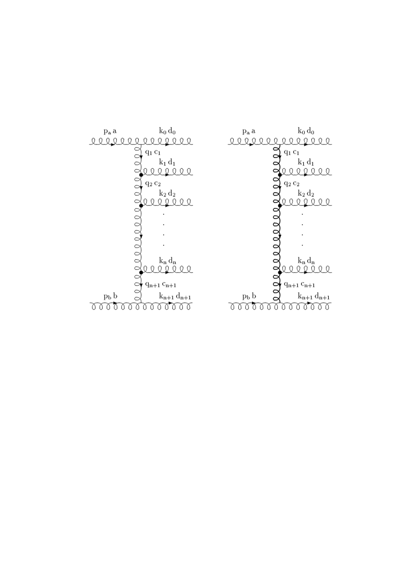
Figure 6: Multigluon amplitude in multiregge kinematics $a)$ at tree level and $b)$ with the virtual radiative corrections, represented by the thicker gluon line. The blobs remind that non-local effective Lipatov vertices are used for the gluon emissions along the ladder.

$$iM^{abd_{0}...d_{n+1}}_{\mu_{a}\mu_{b}\mu_{0}...\mu_{n+1}} \simeq 2i\hat{s}\left(ig_{s}\,f^{ad_{0}c_{1}}\,g_{\mu_{a}\,\mu_{0}}\right)\,{1\over\hat{t}_{1}}$$

$$\cdot \left(ig_{s}\,f^{c_{1}d_{1}c_{2}}\,C^{\mu_{1}}(q_{1},q_{2})\right)\,{1\over\hat{t}_{2}}$$

$$\cdot$$

$$\cdot$$

$$\cdot \left(ig_{s}\,f^{c_{n}d_{n}c_{n+1}}\,C^{\mu_{n}}(q_{n},q_{n+1})\right)\,{1\over\hat{t}_{n+1}}$$

$$\cdot \left(ig_{s}\,f^{bd_{n+1}c_{n+1}}\,g_{\mu_{b}\,\mu_{n+1}}\right),$$

where the Lipatov vertex (80) is

$$C^{\mu}(q_{i},q_{i+1})\simeq\left[(q_{i}+q_{i+1})^{\mu}_{\perp}\,-\,\left({\hat{s}_{ai}\over\hat{s}}\,+\,2{\hat{t}_{i+1}\over\hat{s}_{bi}}\right)p_{b}^{\mu}\,+\left({\hat{s}_{bi}\over\hat{s}}\,+\,2{\hat{t}_{i}\over\hat{s}_{ai}}\right)p_{a}^{\mu}\right].$$ (104)

A proof of the validity of eq.(3.4) may be found in sect. 4 of ref.[46].

Following ref. [24], we make the ansatz that the leading logarithmic approximation (LLA) in $\ln(\hat{s}/\hat{t})$ to the virtual radiative corrections, to all orders in $\alpha_{s}$, is obtained by replacing the propagator for the $i^{th}$ gluon with

$${1\over\hat{t}_{i}}\rightarrow{1\over\hat{t}_{i}}\left(-{\hat{s}_{i-1,i}\over\hat{t}_{i}}\right)^{\alpha(\hat{t}_{i})}={1\over\hat{t}_{i}}e^{\alpha(\hat{t}_{i})(y_{i-1}-y_{i})},$$ (105)

with $\alpha(\hat{t}_{i})$ as in eq.(94). Inserting eq.(105) into eq.(2.4) we obtain the amplitude for the subprocess $gg\rightarrow gg$, with the leading contribution of the virtual corrections to all orders in $\alpha_{s}$,

$$iM^{aba^{\prime}b^{\prime}}_{\mu_{a}\mu_{b}\mu_{a^{\prime}}\mu_{b^{\prime}}}\,=\,-8\pi i\alpha_{s}\,f^{aa^{\prime}c}\,g_{\mu_{a}\,\mu_{a^{\prime}}}\,{\hat{s}\over\hat{t}}\,e^{\alpha(\hat{t})\,(y_{a}-y_{b})}\,f^{bb^{\prime}c}\,g_{\mu_{b}\,\mu_{b^{\prime}}}.$$ (106)

In eq.(102) we have reproduced the calculation of the ${\cal O}(\alpha_{s}^{2})$ term of eq.(106) , the ${\cal O}(\alpha_{s}^{3})$ term has been computed in ref.[24], and in ref.[25] eq.(106) has been conjectured to be valid to all orders in $\alpha_{s}$. This entails that the leading contribution of the virtual radiative corrections to any order in $\alpha_{s}$ has the color-octet structure of one-gluon exchange. Thus, in the decomposition (97) of eq.(106) the only scalar amplitude that contributes to leading $\hat{s}/\hat{t}$ is,

$$A^{oct}(\hat{s},\hat{t})\,=\,-8\pi\alpha_{s}\,N_{c}\,{\hat{s}\over\hat{t}}\,e^{\alpha(\hat{t})\,(y_{a}-y_{b})}.$$ (107)

Replacing eq.(95) into eq.(105) we note that the argument of the exponential factor on the right-hand side is a negative product of a collinear logarithm and a logarithm of type $\ln(\hat{s}/\hat{t})$. This is an example of Sudakov form factor. Accordingly the amplitude (106) and the related production rate are infrared sensitive and vanish as we take $\mu\rightarrow 0$. This infrared behavior is general in gauge theories and was first noticed in QED [48], where the probability for having a scattering process without the emission, or with the emission of a finite number, of soft photons vanishes. It is only after the inclusion of the real radiative corrections that a cross section is well defined and finite order by order in perturbation theory [49].

Inserting then eq.(105) into eq.(3.4), we obtain the multigluon amplitude for the production of $n+2$ gluons, with the leading contribution of the virtual radiative corrections to all orders in $\alpha_{s}$

$$iM^{abd_{0}...d_{n+1}}_{\mu_{a}\mu_{b}\mu_{0}...\mu_{n+1}} \simeq 2i\hat{s}\left(ig_{s}\,f^{ad_{0}c_{1}}\,g_{\mu_{a}\,\mu_{0}}\right)\,{1\over\hat{t}_{1}}e^{\alpha(\hat{t}_{1})\,(y_{0}-y_{1})}$$

$$\cdot \left(ig_{s}\,f^{c_{1}d_{1}c_{2}}\,C^{\mu_{1}}(q_{1},q_{2})\right)\,{1\over\hat{t}_{2}}e^{\alpha(\hat{t}_{2})\,(y_{1}-y_{2})}$$

$$\cdot$$

$$\cdot$$

$$\cdot \left(ig_{s}\,f^{c_{n}d_{n}c_{n+1}}\,C^{\mu_{n}}(q_{n},q_{n+1})\right)\,{1\over\hat{t}_{n+1}}e^{\alpha(\hat{t}_{n+1})\,(y_{n}-y_{n+1})}$$

$$\cdot \left(ig_{s}\,f^{bd_{n+1}c_{n+1}}\,g_{\mu_{b}\,\mu_{n+1}}\right).$$

Eq.(3.4) has been verified for three-gluon production at one loop in ref. [25]. A proof of its validity to all orders in $\alpha_{s}$ may be found in the appendix of ref. [46]. We will follow, though, the original approach of ref. [25], namely we take eq.(3.4) as a corollary of the ansatz (105) and we prove its self-consistency by using eq.(3.4) to derive the elastic amplitude with the virtual radiative corrections in LLA to all orders in $\alpha_{s}$, and by showing that it coincides with eq.(106).

3.5 Partial wawe amplitudes

In this section we derive dispersion relations which will let us reconstruct the elastic amplitude with all the virtual radiative corrections (106).

First, we decompose the scalar amplitude $A^{T}(\hat{s},\hat{t})$ introduced in eq.(97)in $\hat{t}$-channel partial wawe amplitudes

$$A^{T}(\hat{s},\hat{t})=\sum_{l}\,(2l+1)\,A^{T}_{l}(\hat{s},\hat{t})\,P_{l}(z_{t}),$$ (109)

where $l$ is the angular momentum, $P_{l}(z)$ are Legendre polynomials and $z_{t}=-\cos\theta_{t}$ is the scattering angle in the $\hat{t}$-channel physical region, whose Mandelstam invariants are obtained from eq.(19) by crossing the channels $\hat{s}$ and $\hat{t}$,

$$\hat{s} = -{\hat{t}\over 2}(1-\cos\theta_{t}),$$ (110)

$$\hat{u} = -{\hat{t}\over 2}(1+\cos\theta_{t}).$$

Using the invariance of amplitude (97) under the crossing symmetry $\hat{s}\leftrightarrow\hat{u}$,

$$M^{aba^{\prime}b^{\prime}}_{\mu_{a}\mu_{b}\mu_{a^{\prime}}\mu_{b^{\prime}}}(\hat{s},\hat{t},\hat{u})\,=\,M^{ab^{\prime}a^{\prime}b}_{\mu_{a}\mu_{b^{\prime}}\mu_{a^{\prime}}\mu_{b}}(\hat{u},\hat{t},\hat{s})\,,$$ (111)

and the parity of the projectors (100), we obtain the parity of the scalar amplitudes under $\hat{s}\leftrightarrow\hat{u}$ crossing

$$A^{T}(-z_{t},\hat{t})=(-1)^{T}\,A^{T}(z_{t},\hat{t})\,,$$ (112)

with the change of sign of the scattering angle, $z_{t}\leftrightarrow-z_{t}$ under $\hat{s}\leftrightarrow\hat{u}$ crossing, as seen from eq.(110). Next, we write the elastic amplitude (97) through a dispersion relation, i.e. as an integral over the amplitude singularities, which are branch cuts over the real axis of the $\hat{s}$ complex plane, $-\hat{t}\leq\hat{s}<\infty$ for the physical $\hat{s}$ channel, and $-\hat{t}\leq\hat{u}<\infty$ for the physical $\hat{u}$ channel [50],

$$A(\hat{s},\hat{t})=\int_{-\infty}^{0}{ds^{\prime}\over 2\pi i}\,{{\rm Disc}\,A(s^{\prime},\hat{t})\over s^{\prime}-\hat{s}}\,+\,\int_{-\hat{t}}^{\infty}{ds^{\prime}\over 2\pi i}\,{{\rm Disc}\,A(s^{\prime},\hat{t})\over s^{\prime}-\hat{s}}\,,$$ (113)

with

$${\rm Disc}\,A(s^{\prime},\hat{t})=A(s^{\prime}+i\epsilon,\hat{t})-A(s^{\prime}-i\epsilon,\hat{t})\,,$$ (114)

and where we have used $\hat{u}=-\hat{s}-\hat{t}$, and $\hat{t}<0$. Since, from eq.(110),

$$z_{t}=-\left(1+{2\hat{s}\over\hat{t}}\right),$$ (115)

the dispersion relation (113) may be written as an integral over the complex plane of $z_{t}$,

$$A(\hat{s},\hat{t})=\int_{-\infty}^{-1}{dz_{t}^{\prime}\over 2\pi i}\,{{\rm Disc}\,A(z_{t}^{\prime},\hat{t})\over z_{t}^{\prime}-z_{t}}\,+\,\int_{1}^{\infty}{dz_{t}^{\prime}\over 2\pi i}\,{{\rm Disc}\,A(z_{t}^{\prime},\hat{t})\over z_{t}^{\prime}-z_{t}}\,.$$ (116)

We note that in the $\hat{t}$-channel physical region (110), where $z_{t}$ is the scattering angle, $-1\leq z_{t}\leq 1$, while the singularities are at $z_{t}<-1$ and $z_{t}>1$, where the $\hat{t}$ channel is unphysical (116). So at $-1\leq z_{t}\leq 1$ we may invert the partial-wawe expansion (109), to obtain the amplitude for the $l^{th}$ wawe

$$A^{T}_{l}(\hat{s},\hat{t})\,=\,{1\over 2}\int_{-1}^{1}dz_{t}\,P_{l}(z_{t})\,A^{T}(\hat{s},\hat{t})\,.$$ (117)

Introducing the Legendre function, associated to the Legendre polynomial

$$Q_{l}(z^{\prime})\,=\,{1\over 2}\int_{-1}^{1}{dz\over z^{\prime}-z}P_{l}(z)\,,$$ (118)

replacing the dispersion relation (116) into eq.(117), and using the parity under $\hat{s}\leftrightarrow\hat{u}$ crossing,

$$Q_{l}(-z_{t}) = (-1)^{l+1}\,Q_{l}(z_{t})\,,$$ (119)

$${\rm Disc}\,A^{T}(-z_{t},\hat{t}) = (-1)^{T+1}\,{\rm Disc}\,A^{T}(z_{t},\hat{t})\,,$$

the amplitude for the $l^{th}$ wawe becomes

$$A^{T}_{l}(\hat{s},\hat{t})\,=\,\left[1+(-1)^{l+T}\right]\,\int_{1}^{\infty}{dz^{\prime}\over 2\pi i}\,Q_{l}(z^{\prime})\,{\rm Disc}\,A^{T}(z^{\prime},\hat{t})\,.$$ (120)

Next, we introduce the Sommerfeld-Watson representation of the amplitude $A^{T}(\hat{s},\hat{t})$ in the complex plane of the angular momentum $l$ [51],

$$A^{T}(\hat{s},\hat{t})\,=\,\int_{\delta-i\infty}^{\delta+i\infty}{dl\over 2i}\,(2l+1)\,A^{T}_{l}(\hat{s},\hat{t})\,{P_{l}(-z_{t})\over\sin{\pi l}},$$ (121)

where the integral is done along a path parallel to the imaginary axis, to the right of all the singularities. All that we have considered so far in this section describes general properties of the analiticity of the scattering amplitude. Now, we consider the high-energy limit $\hat{s}\rightarrow\infty$ at fixed $\hat{t}$. From eq.(115) we have,

$$z_{t}\rightarrow-{2\hat{s}\over\hat{t}}\,,$$ (122)

and we take the asymptotic value for large $z_{t}$ of the Legendre polynomials and their associated functions [52]

$$P_{l}(z) \rightarrow {1\over\sqrt{\pi}}\,{\Gamma\left(l+{1\over 2}\right)\over\Gamma(l+1)}\,(2z)^{l}\,,$$ (123)

$$Q_{l}(z) \rightarrow \sqrt{\pi}\,{\Gamma(l+1)\over\Gamma\left(l+{3\over 2}\right)}\,(2z)^{-(l+1)}\,.$$

Replacing the amplitude for the $l^{th}$ wawe (120) into the Sommerfeld-Watson representation of the amplitude (121), and using the asymptotics (123), we obtain

$$A^{T}(\hat{s},\hat{t})\,=\,-{1\over 4\pi}\int_{\delta-i\infty}^{\delta+i\infty}dl\,{(-1)^{l}+(-1)^{T}\over\sin{\pi l}}e^{ly}{\cal F}^{T}_{l}(\hat{t})\,,$$ (124)

where ${\cal F}^{T}_{l}(\hat{t})$ is the Laplace transform of the discontinuity of the amplitude

$${\cal F}^{T}_{l}(\hat{t})\,=\,\int_{0}^{\infty}dy\,e^{-ly}\,{\rm Disc}\,A^{T}(z_{t},\hat{t})\,,$$ (125)

with $y=\ln{(z_{t}/2)}$.

3.6 The BFKL equation

Our goal is now to use the $\hat{s}$-channel unitarity and the multigluon amplitude with exchange of one gluon in the $\hat{t}$ channel (3.4) to evaluate the discontinuity of the amplitude for exchange of two gluons in the $\hat{t}$ channel in a physical gauge. From that by using the dispersion relations computed above the elastic amplitude with all the virtual radiative corrections (106) will be derived.

In order to evaluate the discontinuity of the amplitude, we compute and sum over $n$ the cut diagram of Fig.7. In evaluating the diagram at $n+1$ loops, we must put the internal legs $k_{i}$ on mass shell, by replacing the $n+2$ internal propagators with the cut ones [53]

$${i\over k_{i}^{2}}\rightarrow 2\pi\,\delta(k_{i}^{2})\,.$$ (126)

Multiplying then the mass-shell factors (126) by the $n+1$ loop-momentum integrals, we obtain the phase space for the production of $n+2$ partons

$${\cal P}_{n+2}\equiv\prod_{i=0}^{n}\int{d^{4}k_{i}\over(2\pi)^{4}}\,\prod_{j=0}^{n+1}2\pi\,\delta(k^{2}_{j})\,=\,\prod_{i=0}^{n+1}\int{dy_{i}\,d^{2}k_{i\perp}\over 4\pi(2\pi)^{2}}\,(2\pi)^{4}\,\delta^{4}(p_{a}+p_{b}-\sum_{i=0}^{n+1}k_{i})$$ (127)

where we have inserted the identity $\int d^{4}k_{n+1}\delta^{4}(p_{a}+p_{b}-\sum_{i=0}^{n+1}k_{i})=1$, and used eq.(14). Now we need to consider the phase space in the multiregge kinematics. This has already been computed for three-parton production in eq.(86). Since light-cone momentum conservation in the multiregge kinematics (68) has the same form for three or more partons, eq.(86) trivially generalizes to $n+2$ partons, and the phase space (127) becomes,

$${\cal P}_{n+2}=\int{1\over 2\hat{s}}\,{d^{2}k_{0\perp}\over(2\pi)^{2}}\,\left(\prod_{i=1}^{n}{dy_{i}\,d^{2}k_{i\perp}\over 4\pi(2\pi)^{2}}\right)\,{d^{2}k_{n+1\perp}\over(2\pi)^{2}}\,(2\pi)^{2}\,\delta^{2}\left(\sum_{i=0}^{n+1}k_{i\perp}^{2}\right)\,.$$ (128)

Figure 7: ${\cal O}(\alpha_{s}^{n+2})$ contribution to the discontinuity of the elastic amplitude with two-gluon ladder exchange in the $\hat{t}$ channel.

Then using eq.(3.4) the discontinuity of the amplitude of Fig.7 is

$${\rm Disc}\left[iM^{aba^{\prime}b^{\prime}}_{\mu_{a}\mu_{b}\mu_{a^{\prime}}\mu_{b^{\prime}}}(\hat{s},\hat{t})\right]\,=$$

$$\sum_{n=0}^{\infty}\int{1\over 2\hat{s}}\,{d^{2}k_{0\perp}\over(2\pi)^{2}}\,\left(\prod_{i=1}^{n}{dy_{i}\,d^{2}k_{i\perp}\over 4\pi(2\pi)^{2}}\right)\,{d^{2}k_{n+1\perp}\over(2\pi)^{2}}\,(2\pi)^{2}\,\delta^{2}\left(\sum_{i=0}^{n+1}k_{i\perp}^{2}\right)$$

$$\cdot (2i\hat{s})^{2}\,\delta_{\perp}^{\mu_{a}\mu_{a^{\prime}}}\,\delta_{\perp}^{\mu_{b}\,\mu_{b^{\prime}}}\,\left(ig_{s}\,f^{ad_{0}c_{1}}\right)\,\left(ig_{s}\,f^{c^{\prime}_{1}d_{0}a^{\prime}}\right)$$

$$\cdot {1\over\hat{t}_{1}}e^{\alpha(\hat{t}_{1})\,(y_{0}-y_{1})}\,{1\over\hat{t}^{\prime}_{1}}e^{\alpha(\hat{t}^{\prime}_{1})\,(y_{0}-y_{1})}$$

$$\cdot \left(ig_{s}\,f^{c_{1}d_{1}c_{2}}\right)\,\left(ig_{s}\,f^{c^{\prime}_{1}d_{1}c^{\prime}_{2}}\right)\,C^{\mu_{1}}(q_{1},q_{2})(-g_{\mu_{1}\mu^{\prime}_{1}})C^{\mu^{\prime}_{1}}(q-q_{1},q-q_{2})$$

$$\cdot {1\over\hat{t}_{2}}e^{\alpha(\hat{t}_{2})\,(y_{1}-y_{2})}\,{1\over\hat{t}^{\prime}_{2}}e^{\alpha(\hat{t}^{\prime}_{2})\,(y_{1}-y_{2})}$$

$$\cdot$$

$$\cdot$$

$$\cdot \left(ig_{s}\,f^{c_{n}d_{n}c_{n+1}}\right)\,\left(ig_{s}\,f^{c^{\prime}_{n}d_{n}c^{\prime}_{n+1}}\right)\,C^{\mu_{n}}(q_{n},q_{n+1})(-g_{\mu_{n}\mu^{\prime}_{n}})C^{\mu^{\prime}_{n}}(q-q_{n},q-q_{n+1})$$

$$\cdot {1\over\hat{t}_{n+1}}e^{\alpha(\hat{t}_{n+1})\,(y_{n}-y_{n+1})}\,{1\over\hat{t}^{\prime}_{n+1}}e^{\alpha(\hat{t}^{\prime}_{n+1})\,(y_{n}-y_{n+1})}$$

$$\cdot \left(ig_{s}\,f^{bd_{n+1}c_{n+1}}\right)\left(ig_{s}\,f^{c^{\prime}_{n+1}d_{n+1}b^{\prime}}\right)\,,$$

where $\hat{t}=q^{2}$ is the momentum transfer in the elastic scattering and $\hat{t}^{\prime}_{i}=(q-q_{i})^{2}$. In eq.(3.6) we have used the phase space (128), and we have done the sum over the helicities of the gluons emitted from the helicity-conserving vertices using eq.(42), and the ones over the $n$ intermediate gluons using eq.(46) since the Lipatov vertices are gauge invariant (81). The Lipatov vertex $C^{\mu^{\prime}_{i}}(q-q_{i},q-q_{i+1})$ in eq.(3.6) may be obtained either by direct construction as in sect. 3.2 or by simply inverting the sign of the momentum $k_{i}$ in eq.(104),

$$C^{\mu}(q-q_{i},q-q_{i+1})\simeq\left[\left((q-q_{i})\,+\,(q-q_{i+1})\right)^{\mu}_{\perp}\,+\,\left({\hat{s}_{ai}\over\hat{s}}\,+\,2{\hat{t}^{\prime}_{i+1}\over\hat{s}_{bi}}\right)p_{b}^{\mu}\,-\left({\hat{s}_{bi}\over\hat{s}}\,+\,2{\hat{t}^{\prime}_{i}\over\hat{s}_{ai}}\right)p_{a}^{\mu}\right].$$ (130)

Then using eq.(71), (104), (130) and the kinematic constraint $\hat{s}_{ai}\hat{s}_{bi}=k_{i\perp}^{2}\hat{s}$ from eq.(66), with $k_{i\perp}^{2}=(q_{i}-q_{i+1})_{\perp}^{2}$, the contraction of the Lipatov vertices becomes

$$C^{\mu}(q_{i},q_{i+1})\,C_{\mu}(q-q_{i},q-q_{i+1})\, = -2\left[q_{\perp}^{2}\,-\,{(q-q_{i})_{\perp}^{2}q_{i+1\perp}^{2}+(q-q_{i+1})_{\perp}^{2}q_{i\perp}^{2}\over(q_{i}-q_{i+1})_{\perp}^{2}}\right]$$ (131)

$$\equiv -2{\cal K}(q_{i},q_{i+1})\,.$$

Next, using eq.(97) we consider the scalar part ${\rm Disc}A^{T}(\hat{s},\hat{t})$ of the discontinuity (3.6). The contraction of the color projectors (99) with the structure constants in eq.(3.6) yields the color factor $C_{T}^{n+2}$, with

$$C_{T}=\left\{\begin{array}[]{ll}N_{c}&\mbox{for the {\sl singlet}},\\ {N_{c}/2}&\mbox{for the {\sl octet}},\end{array}\right.$$ (132)

where we have used the Jacobi identity (77) in the contraction with the octet projector. So the scalar part of the discontinuity (3.6) may be written using eq.(131) and (132) as,

$${\rm Disc}A^{T}(\hat{s},\hat{t}) = \sum_{n=0}^{\infty}\left(-g_{s}^{2}C_{T}\right)^{n+2}\int\prod_{i=1}^{n}{dy_{i}\over 4\pi}\,\prod_{j=1}^{n+1}{d^{2}q_{j\perp}\over(2\pi)^{2}}\,$$ (133)

$$\cdot 2i\,\hat{s}\,\prod_{l=1}^{n+1}{1\over\hat{t}_{l}\hat{t}^{\prime}_{l}}\,e^{(y_{l-1}-y_{l})[\alpha(\hat{t}_{l})+\alpha(\hat{t}^{\prime}_{l})]}\,\prod_{m=1}^{n}2{\cal K}(q_{m},q_{m+1})\,,$$

where we have used the conservation of the transverse momentum and we have changed integration variables from the transverse components of the produced gluons to the ones of the gluons exchanged in the $\hat{t}$ channel. In eq.(133) we have $n$ integrations over the rapidities of the gluons emitted within the ladder, while in the integrand there are $n+1$ rapidity differences. To disentangle the integrations, we take the Laplace transform (125) of eq.(133) with respect to the rapidity difference $y=y_{0}-y_{n+1}=\ln{(-\hat{s}/\hat{t})}$, and change the integrations over the rapidities $y$ and $y_{i}$, with $i=1,...,n$ to the ones over the rapidity differences $y_{i-1}-y_{i}$, with $i=1,...,n+1$. Then we perform the integrations, with boundaries given by the strong rapidity ordering (65), and we obtain

$${\cal F}^{T}_{l}(\hat{t}) = -2i\,\hat{t}\,(4\pi\alpha_{s})^{2}\,C_{T}^{2}\,\sum_{n=0}^{\infty}\int\prod_{j=1}^{n+1}{d^{2}q_{j\perp}\over(2\pi)^{2}}\,$$

$$\cdot {1\over\hat{t}_{1}\hat{t}^{\prime}_{1}}\,{1\over l-1-\alpha(\hat{t}_{1})-\alpha(\hat{t}^{\prime}_{1})}$$

$$\cdot (-2\alpha_{s}C_{T})\,{\cal K}(q_{1},q_{2})$$

$$\cdot {1\over\hat{t}_{2}\hat{t}^{\prime}_{2}}\,{1\over l-1-\alpha(\hat{t}_{2})-\alpha(\hat{t}^{\prime}_{2})}$$

$$\cdot$$

$$\cdot$$

$$\cdot (-2\alpha_{s}C_{T})\,{\cal K}(q_{n},q_{n+1})$$

$$\cdot {1\over\hat{t}_{n+1}\hat{t}^{\prime}_{n+1}}\,{1\over l-1-\alpha(\hat{t}_{n+1})-\alpha(\hat{t}^{\prime}_{n+1})}\,.$$

This may be written as a recursive relation,

$${\cal F}^{T}_{l}(\hat{t})\,=\,-2i\,\hat{t}\,(4\pi\alpha_{s})^{2}\,C_{T}^{2}\,\int{d^{2}q_{1\perp}\over(2\pi)^{2}}\,{1\over q_{1\perp}^{2}(q-q_{1})_{\perp}^{2}}\,f_{l}^{T}(q_{1},\hat{t})\,,$$ (135)

where the function $f_{l}^{T}(q,\hat{t})$ satisfies the integral equation,

$$\left[l-1-\alpha(\hat{t}_{1})-\alpha(\hat{t}^{\prime}_{1})\right]f_{l}^{T}(q_{1},\hat{t})\,=\,1-2\alpha_{s}C_{T}\int{d^{2}q_{2\perp}\over(2\pi)^{2}}\,{{\cal K}(q_{1},q_{2})\over q_{2\perp}^{2}(q-q_{2})_{\perp}^{2}}\,f_{l}^{T}(q_{2},\hat{t})\,,$$ (136)

with $\hat{t}_{i}=-q_{i\perp}^{2}$ and $\hat{t}^{\prime}_{i}=-(q-q_{i})_{\perp}^{2}$. Eq.(136) is the BFKL integral equation [25], describing the gluon-ladder evolution in the LLA of $\ln{(\hat{s}/\hat{t})}$. The function ${\cal K}(q_{1},q_{2})$, defined as the contraction of the Lipatov vertices (131), describes the contribution of the real radiative corrections and forms the kernel of the BFKL equation. The contribution of the virtual radiative corrections $\alpha(\hat{t})$ appears on the left-hand side of eq.(136).

Next, we are going to solve the BFKL equation for the color-octet exchange. Replacing then eq.(132) and the explicit form (94) of $\alpha(\hat{t})$ into eq.(136), this reduces to

$$(l-1)\,f_{l}^{oct}(q_{1},\hat{t})\,=\,1-\alpha_{s}N_{c}\,q_{\perp}^{2}\int{d^{2}k_{\perp}\over(2\pi)^{2}}\,{1\over k_{\perp}^{2}(q-k)_{\perp}^{2}}\,f_{l}^{oct}(k,\hat{t})\,,$$ (137)

which admits the solution

$$f_{l}^{oct}(q_{1},\hat{t})\,=\,f_{l}^{oct}(k,\hat{t})\,=\,{1\over l-1-\alpha(\hat{t})}\,.$$ (138)

The solution is unique, since eq.(136) is inhomogeneous, and it is constant with respect to the functional dependence from its first argument. Replacing eq.(138) into the Laplace transform (135) and using eq.(94) and (132), we obtain

$${\cal F}^{oct}_{l}(\hat{t})\,=\,-8\pi^{2}i\,N_{c}\,\alpha_{s}\,{\alpha(\hat{t})\over l-1-\alpha(\hat{t})}\,.$$ (139)

Replacing eq.(139) into the Sommerfeld-Watson representation of amplitude (124) and using the parity factor (101), the scalar part of the amplitude for octet exchange becomes

$$A^{oct}(\hat{s},\hat{t})\,=\,4\pi\,N_{c}\,\alpha_{s}\,{\pi\alpha(\hat{t})\over\sin{\pi\alpha(\hat{t})}}\,\left(1+e^{i\pi\alpha(\hat{t})}\right)\,\left(\hat{s}\over-\hat{t}\right)^{1+\alpha(\hat{t})}\,,$$ (140)

where the integral over the complex plane of $l$ has yielded a Regge pole at $l=1+\alpha(\hat{t})$, which then gives the Regge trajectory $\hat{s}^{1+\alpha(\hat{t})}$. Since $\alpha(\hat{t}=0)=0$, the intercept is at $l=1$, which corresponds to a reggeized gluon [25], [51].

Even though we started with a discontinuity (3.6) at ${\cal O}(\alpha_{s}^{2})$, that computes the radiative corrections due the insertion of a two-gluon ladder, the octet solution (140) is ${\cal O}(\alpha_{s})$, because the octet appears already at the one-gluon exchange level.

Finally, we note that in the multiregge region (65), where the collinear logarithms are not supposed to be large, $\alpha_{s}\ln{(q_{\perp}^{2}/\mu^{2})}\ll 1$. Then from eq.(95) we obtain that $\pi|\alpha(\hat{t})|\ll 1$. Taking this limit in eq.(140), we find it in agreement with eq.(107), proving thereby the self-consistency of the ansatz (105) for eq.(106) [25].

3.7 The pomeron solution

We are now interested to study the singlet solution of the BFKL equation (136), since it can be related via the optical theorem to the total cross section for one-gluon exchange in the $\hat{t}$ channel. Let us write first the function $f_{l}^{sing}(q_{1},\hat{t})$ in differential form,

$$f_{l}^{sing}(q_{1},\hat{t})\,=\,\int{d^{2}k_{\perp}\over(2\pi)^{2}}{\bar{f}}_{l}(q_{1},k,\hat{t})\,.$$ (141)

Replacing it into eq.(136) and using eq.(132), we obtain the BFKL equation for color-singlet exchange,

$$\left[l-1-\alpha(\hat{t}_{1})-\alpha(\hat{t}^{\prime}_{1})\right]{\bar{f}}_{l}(q_{1},k,\hat{t})\,=$$

$$(2\pi)^{2}\,\delta^{2}(q_{1}-k)\,-\,2\alpha_{s}N_{c}\,\int{d^{2}q_{2\perp}\over(2\pi)^{2}}\,{{\cal K}(q_{1},q_{2})\over q_{2\perp}^{2}(q-q_{2})_{\perp}^{2}}\,{\bar{f}}_{l}(q_{2},k,\hat{t})\,.$$ (142)

Since by pomeron exchange it is meant conventionally the exchange of something with quantum numbers of the vacuum, the exchange of a two-gluon ladder in a color-singlet configuration defines the exchange of a perturbative QCD pomeron.

The kernel ${\cal K}(q_{1},q_{2})$ (131) is regular as $q^{2}_{2\perp}\rightarrow\infty$, making the right-hand side of eq.(142) ultraviolet finite. There are ultraviolet divergences as $q^{2}_{1\perp}\rightarrow\infty$ in the virtual radiative corrections (95) in the left-hand side of eq.(142), but they cancel in the singlet solution (135). As for the infrared behavior of eq.(142), the kernel vanishes at $q_{2\perp}^{2}=0$, or at $(q-q_{2})_{\perp}^{2}=0$, where accordingly the right-hand side of eq.(142) is regular. The kernel is singular at $q_{1}^{2}=q_{2}^{2}$, however making the substitution

$$\int d^{2}q_{2}{q_{1\perp}^{2}\over q_{2\perp}^{2}(q_{1}-q_{2})_{\perp}^{2}}\,=\,2\,\int d^{2}q_{2}{q_{1\perp}^{2}\over\left[q_{2\perp}^{2}+(q_{1}-q_{2})_{\perp}^{2}\right]\,(q_{1}-q_{2})_{\perp}^{2}}\,,$$ (143)

in the virtual radiative-corrections terms of eq.(142), it is easy to see that the singularity at $q_{1}^{2}=q_{2}^{2}$ cancels between the virtual and real radiative corrections. Still, eq.(142) has infrared divergences as $q_{1}^{2}\rightarrow 0$ in the virtual radiative corrections. Besides, at $q_{1\perp}^{2}=0$ or $(q-q_{1})_{\perp}^{2}=0$ the kernel vanishes, and after using eq.(141), eq.(142) reduces to eq.(137), thus the two-gluon ladder reduces to a one-gluon ladder, which is infrared sensitive as we know from sect.3.4 and 3.6. However, it is possible to show that in particular cases, like for the exchange of a singlet gluon ladder between colorless objects, the solution of eq.(142) has no infrared divergences at all [54].

Since we are interested in the forward scattering amplitude and in the total cross section, we look for the solution of eq.(142) at $q=0$. From eq.(82) and (131) we obtain

$${\cal K}(q_{1},q_{2})|_{q=0}\,=\,-2\,{q_{1\perp}^{2}q_{2\perp}^{2}\over(q_{1}-q_{2})_{\perp}^{2}}\,.$$ (144)

Doing then the substitution of variables,

$$f_{l}(q_{1},k)\,=\,{1\over 8\pi^{2}}\,{k_{\perp}^{2}\over q_{1\perp}^{2}}\,{\bar{f}}_{l}(q_{1},k,\hat{t}=0)\,,$$ (145)

the BFKL equation for singlet exchange at $\hat{t}=0$ becomes

$$(l-1)\,f_{l}(q_{1},k)\,=$$ (146)

$${1\over 2}\,\delta^{2}(q_{1}-k)\,+\,{\alpha_{s}N_{c}\over\pi^{2}}\int d^{2}q_{2\perp}\,{1\over(q_{1}-q_{2})_{\perp}^{2}}\,\left[f_{l}(q_{2},k)-{q_{1\perp}^{2}\over 2q_{2\perp}^{2}}\,f_{l}(q_{1},k)\right]\,.$$

This is a inhomogeneous integral equation with a self-adjoint kernel, given by the real radiative corrections to the discontinuity of the amplitude. As we have done for eq.(142), in order to regulate the divergence at $q_{1}^{2}=q_{2}^{2}$ we make the substitution (143) in the virtual radiative-corrections term on the right-hand side of eq.(146) (cf. Appendix A), then the BFKL equation at $\hat{t}=0$ reads

$$(l-1)\,f_{l}(q_{1},k)\,=$$ (147)

$${1\over 2}\,\delta^{2}(q_{1}-k)\,+\,{\alpha_{s}N_{c}\over\pi^{2}}\int d^{2}q_{2\perp}\,{1\over(q_{1}-q_{2})_{\perp}^{2}}\,\left[f_{l}(q_{2},k)-{q_{1\perp}^{2}\over q_{2\perp}^{2}+(q_{1}-q_{2}){\perp}^{2}}\,f_{l}(q_{1},k)\right]\,.$$

The homogeneous equation associated to eq.(147), may be written as

$$(l-1)\,f_{l}(q_{1},k)\,=$$ (148)

$${\alpha_{s}N_{c}\over\pi^{2}}\int d^{2}q_{2\perp}\,\left\{{f_{l}(q_{2},k)\over(q_{1}-q_{2})_{\perp}^{2}}\,-\,{q_{1\perp}^{2}\over q_{2\perp}^{2}}\left[{1\over(q_{1}-q_{2})_{\perp}^{2}}\,-\,{1\over q_{2\perp}^{2}+(q_{1}-q_{2})_{\perp}^{2}}\right]\,f_{l}(q_{1},k)\right\}\,,$$

and admits a solution as a Fourier series

$$f_{l}(q_{1},k)\,=\,\sum_{n=-\infty}^{\infty}\,\int_{-\infty}^{\infty}d\nu\,a(\nu,n)\,e^{i\nu(\lambda_{1}-\lambda)}\,e^{in(\phi_{1}-\phi)}\,,$$ (149)

with $\lambda_{1}=\ln(q_{1}^{2}/m^{2})$, $\lambda=\ln(k^{2}/m^{2})$, $m^{2}$ a scale factor, and $\phi_{1}-\phi$ the azimuthal angle between the vectors $k_{\perp}$ and $q_{1\perp}$. Using then the integral representation of the $\delta$-function, the inhomogeneous term in eq.(147) can be expanded as

$$\delta^{2}(q_{1}-k)\,=\,{1\over(k_{\perp}^{2}q_{1\perp}^{2})^{1/2}}\,{1\over 2\pi^{2}}\,\sum_{n=-\infty}^{\infty}\int_{-\infty}^{\infty}d\nu\,e^{i\nu(\lambda_{1}-\lambda)}\,e^{in(\phi_{1}-\phi)}\,.$$ (150)

Replacing eq.(150) into eq.(147) and calling $\omega(\nu,n)$ the eigenvalue of the homogeneous equation (148), we obtain the condition

$$(l-1)\,a(\nu,n)\,=\,{1\over(k_{\perp}^{2}q_{1\perp}^{2})^{1/2}}\,{1\over(2\pi)^{2}}\,+\,\omega(\nu,n)a(\nu,n)\,,$$ (151)

which fixes the coefficient $a(\nu,n)$ in the solution (149),

$$f_{l}(q_{1},k)\,=\,{1\over(2\pi)^{2}}\,{1\over(k_{\perp}^{2}q_{1\perp}^{2})^{1/2}}\,\sum_{n=-\infty}^{\infty}\int_{-\infty}^{\infty}d\nu\,{1\over l-1-\omega(\nu,n)}\,e^{i\nu(\lambda_{1}-\lambda)}\,e^{in(\phi_{1}-\phi)}\,.$$ (152)

To find the spectrum of eigenvalues, we replace the solution (152) into the homogeneous equation (148), and obtain

$$\omega(\nu,n)\, = {\alpha_{s}N_{c}\over\pi}\,\left[2\,{\rm Re}\int_{0}^{1}dx\,{x^{{|n|-1\over 2}+i\nu}\over 1-x}-2\int_{0}^{1}dx\,{1\over 1-x}\right.$$ (153)

$$\left.-\,\int_{0}^{1}dx\,{1\over x}\,+\,\int_{0}^{1}dx\,{1\over x\sqrt{1+4x^{2}}}\,+\,\int_{0}^{1}dx\,{1\over\sqrt{x^{2}+4}}\right]\,,$$

with

$$x=\,\left\{\begin{array}[]{ll}q_{2}^{2}/q_{1}^{2}&\mbox{for $q_{2}^{2}<q_{1}^{2}$}\,,\\ q_{1}^{2}/q_{2}^{2}&\mbox{for $q_{2}^{2}>q_{1}^{2}$}\,.\end{array}\right.$$ (154)

The last three terms in eq.(153) cancel out, and introducing the logarithmic derivative of the $\Gamma$ function

$${d\ln{\Gamma(y)}\over dy}\,=\,\psi(y)\,=\,\int_{0}^{1}dx{x^{y-1}-1\over x-1}-\gamma\,,$$ (155)

with $\gamma=-\psi(1)=0.577215...$ the Euler-Mascheroni constant, the eigenvalue (153) becomes

$$\omega(\nu,n)\,=\,-2{\alpha_{s}N_{c}\over\pi}\,{\rm Re}\left[\psi\left({|n|+1\over 2}+i\nu\right)-\psi(1)\right]\,.$$ (156)

$\omega(\nu,n)$ is regular at both the integration limits (155), entailing that eq.(147) is regular at $q_{2}^{2}=0$, $q_{2}^{2}=q_{1}^{2}$, and $q_{2}^{2}\rightarrow\infty$, i.e. that all the infrared and ultraviolet divergences cancel out.

Next, we use the solution (152) in the Laplace transform of the discontinuity of the amplitude (135). The right-hand side of eq.(135) is proportional to $\hat{t}$, so it seems to vanish. However, the factor $\hat{t}$ was due to replacing $\hat{s}=-\hat{t}e^{y_{0}-y_{n+1}}$ into eq.(133), and for the $\hat{t}=0$ case we should have rather done the substitution $\hat{s}=k_{\perp}^{2}e^{y_{0}-y_{n+1}}$, with $k_{\perp}^{2}$ as in eq.(65). Doing so, and using eq.(132), (141) and (145), the Laplace transform of the discontinuity for singlet exchange becomes

$${\cal F}^{sing}_{l}(\hat{t}=0)\,=\,16i\,k_{\perp}^{2}\,\alpha_{s}^{2}\,N_{c}^{2}\,\int d^{2}k_{a\perp}\,d^{2}k_{b\perp}\,{1\over k_{a\perp}^{2}k_{b\perp}^{2}}f_{l}(k_{a},k_{b})\,,$$ (157)

with $f_{l}(k_{a},k_{b})$ as in eq.(152), with eigenvalue (156). Before taking the inverse Laplace transform of eq.(157),

$${\rm Disc}A(\hat{s},\hat{t})\,=\,\int{dl\over 2\pi i}e^{ly}{\cal F}_{l}(\hat{t})\,,$$ (158)

it is convenient to examine the eigenvalue (156) to determine where the leading singularity at large $y$ is. The leading contribution to $\omega(\nu,n)$ comes from $n=\nu=0$ (cf. Appendix B), and for small $\nu$ the eigenvalue admits the expansion (189)

$$\omega(\nu,n=0)\,=\,2{\alpha_{s}N_{c}\over\pi}\,\left(2\ln{2}-7\zeta(3)\,\nu^{2}\,+\,...\right)\,.$$ (159)

Replacing it into eq.(152), and evaluating the integral over the complex plane of $\nu$, we obtain the leading contribution to the solution for the singlet,

$$f_{l}(k_{a},k_{b})\,\simeq\,{1\over(2\pi)^{2}}\,{1\over(k_{a\perp}^{2}k_{b\perp}^{2})^{1/2}}\,{\pi\over\left[B(l-1-A)\right]^{1/2}}\,e^{-\nu_{0}|\ln({k_{a\perp}^{2}/k_{b\perp}^{2}})|}\,.$$ (160)

with

$$A\,=\,4\ln{2}\,{\alpha_{s}N_{c}\over\pi}\,;\qquad B\,=\,14\zeta(3)\,{\alpha_{s}N_{c}\over\pi}\,;\qquad\nu_{0}\,=\,\left({l-1-A\over B}\right)^{1/2}\,.$$ (161)

Replacing it into the discontinuity (158), we see that in the complex plane of $l$ the leading singularity of the pomeron solution is a branch cut, extending from $-\infty$ up to $l=1+A$ [26].

Now, let us go back to the full solution (152). Taking the inverse Laplace transform (158) of eq.(157) and using eq.(152), the discontinuity of the amplitude for singlet exchange is

$${\rm Disc}A^{sing}(\hat{s},\hat{t}=0)\,=\,16i\,\hat{s}\,\alpha_{s}^{2}\,N_{c}^{2}\,\int d^{2}q_{a\perp}\,d^{2}q_{b\perp}\,{1\over q_{a\perp}^{2}q_{b\perp}^{2}}f(q_{a},q_{b},y)\,,$$ (162)

with $y=\ln{(\hat{s}/k_{\perp}^{2})}$ and,

$$f(q_{a},q_{b},y)\,=\,{1\over(2\pi)^{2}}\,{1\over(q_{a\perp}^{2}q_{b\perp}^{2})^{1/2}}\,\sum_{n=-\infty}^{\infty}e^{in\bar{\phi}}\,\int_{-\infty}^{\infty}d\nu\,e^{\omega(\nu,n)y}\,e^{i\nu\ln(q_{a\perp}^{2}/q_{b\perp}^{2})}\,,$$ (163)

with $\bar{\phi}$ the azimuthal angle between the vectors $q_{a\perp}$ and $q_{b\perp}$, corresponding to the first and the last gluon momenta exchanged on the ladder (Fig.8). $f(q_{a},q_{b},y)$ may be also written as the inverse Laplace transform of the solution (152) with respect to $\omega=l-1$.

Next, we consider unitarity and the optical theorem to relate the total cross section for gluon-gluon scattering with exchange of a one-gluon ladder (Fig.6b) to the forward amplitude for gluon-gluon elastic scattering with exchange of a two-gluon ladder (Fig.7),

$$\hat{\sigma}_{tot}\,=\,{1\over 2\hat{s}}\,\int d{\cal P}M\,M^{\dagger}\,=\,-{1\over 2\hat{s}}\,{\rm Disc}\left[i{\overline{M}}(\hat{s},\hat{t}=0)\right]\,,$$ (164)

with ${\cal P}$ the phase space of eq.(127), and where we have used eq.(114). ${\overline{M}}(\hat{s},\hat{t}=0)$ is the forward amplitude summed (averaged) over final (initial) colors and helicities. From eq.(97) it can be written as

$${\overline{M}}(\hat{s},\hat{t})\,=\,{1\over N_{c}^{2}-1}\,A^{sing}(\hat{s},\hat{t})\,.$$ (165)

Using then eq.(162) and (165), the total cross section for gluon-gluon scattering (164) in multiregge kinematics is given by [27]

$$\hat{\sigma}_{tot}\,=\,{8N_{c}^{2}\over N_{c}^{2}-1}\,\alpha_{s}^{2}\,\int d^{2}k_{a\perp}\,d^{2}k_{b\perp}\,{1\over k_{a\perp}^{2}k_{b\perp}^{2}}f(k_{a},k_{b},y)\,,$$ (166)

with $k_{a\perp}=-q_{a\perp}$ and $k_{b\perp}=q_{b\perp}$, as in Fig.8. $f(k_{a},k_{b},y)$ is given by eq.(163) with $\phi=\bar{\phi}+\pi$ the azimuthal angle between the vectors $k_{a\perp}$ and $k_{b\perp}$, and $y=\ln{(\hat{s}/k_{a\perp}k_{b\perp})}$ the rapidity interval between gluons $k_{a}$ and $k_{b}$.

Figure 8: Two-gluon production with exchange of a BFKL ladder, represented schematically by the double-lined square.

As noted after eq.(156), the solution (152) or (163) of the BFKL equation for singlet exchange at $\hat{t}=0$ has no infrared and ultraviolet divergences. Namely, the doubly logarithmic enhancements of the virtual and real radiative corrections cancel out, leaving as a residue single logarithms. Accordingly, the expansion of eq.(163) is finite order by order in $\alpha_{s}$. This is due to the optical theorem (164) which relates the forward scattering amplitude to the total cross section, for which all the infrared and ultraviolet logarithmic divergences in the radiative corrections to the Born amplitude cancel out, order by order in $\alpha_{s}$. Besides, as discussed at the end of sect. 3.3 the coupling constant $\alpha_{s}$ in eq.(147) must be regarded as fixed, thus the total cross section (166) does not depend on a renormalization scale $\mu$. Finally, we note that because of the leading singularity (160) at $l=1+A$, the growth of the total cross section, $\hat{\sigma}_{tot}\,=\,\hat{s}^{A}$, violates the Froissart unitarity bound $\sigma_{tot}\propto\ln^{2}{s}$ [51].

3.8 The total parton cross section

Summarizing the conclusions of sect.3.7, the parton cross section for the production of two gluons, resummed to all orders of $\alpha_{s}\ln{(\hat{s}/k_{\perp}^{2})}$, is obtained from eq.(163) and (166),

$${d\hat{\sigma}_{gg}\over d^{2}k_{a\perp}d^{2}k_{b\perp}}\ =\ \biggl{[}{C_{A}\alpha_{s}\over k_{a\perp}^{2}}\biggr{]}\,f(k_{a},k_{b},y)\,\biggl{[}{C_{A}\alpha_{s}\over k_{b\perp}^{2}}\biggr{]}\ ,$$ (167)

with $y=y_{a}-y_{b}$ and $f(k_{a},k_{b},y)$ the inverse Laplace transform of the singlet solution $f_{l}(k_{a},k_{b})$ (152),

$$f(k_{a},k_{b},y)\,=\,\int{d\omega\over 2\pi i}\,e^{\omega y}\,f_{l}(k_{a},k_{b})\,,$$ (168)

with $\omega=l-1$. Eq.(167) is written as a convolution of the singlet solution (168) with the parton-production vertices on each side of the rapidity interval. The structure of eq.(167) is generic and valid for any scattering process in multiregge kinematics (cf. Appendix C).

First, we consider the limit $\alpha_{s}y\rightarrow 0$ in eq.(167), for which all the real and virtual radiative corrections vanish, and the singlet solution (168) reduces to the inhomogeneous term of the BFKL equation,

$$f(k_{a},k_{b},y)|_{{\cal O}(\alpha_{s}^{0})}\,=\,\delta(k_{a\perp}^{2}-k_{b\perp}^{2})\,\delta(\phi-\pi)\,,$$ (169)

i.e. at the Born level only two partons are produced, and they are balanced in $k_{\perp}$ and back-to-back in $\phi$, and eq.(167) reduces to the Born parton cross section (54).

By integrating eq.(167) over the azimuthal angle only the $n=0$ contribution to the eigenvalue (156) survives

$${d\hat{\sigma}_{gg}\over dk_{a\perp}^{2}dk_{b\perp}^{2}}\ =\ {C_{A}^{2}\alpha_{s}^{2}\over 4k_{a\perp}^{3}k_{b\perp}^{3}}\,\int_{-\infty}^{\infty}d\nu\,e^{\omega(\nu,n=0)y}\ e^{i\nu\ln(k_{a\perp}^{2}/k_{b\perp}^{2})}\,.$$ (170)

In the asymptotic limit of large rapidities, we may approximate the eigenvalue (156) with its expansion (159) at small $\nu$, and perform the integral over $\nu$ by the saddle-point method,

$${d\hat{\sigma}_{gg}\over dk_{a\perp}^{2}dk_{b\perp}^{2}}\ =\ {\pi C_{A}^{2}\alpha_{s}^{2}\over 4k_{a\perp}^{3}k_{b\perp}^{3}}\,{e^{Ay}\over\sqrt{\pi By}}\,\exp\left(-{\ln^{2}(k_{a\perp}^{2}/k_{b\perp}^{2})\over 4By}\right)\,,$$ (171)

with $A$ and $B$ given in eq.(161). Eq.(171) shows a diffusion pattern, namely it has the form of a Gaussian distribution in $\ln(k_{a\perp}^{2}/k_{b\perp}^{2})$ with the peak positioned where the partons are balanced in $k_{\perp}$ and with a width growing with $y$. This is not accidental, since the BFKL equation may be written as a diffusion equation, with diffusion rate $\ln(k_{a\perp}^{2}/k_{b\perp}^{2})\sim y^{1/2}$ (cf. Appendix D).

Let us go back to eq.(170), and perform the integration over the parton transverse momenta above a cutoff $p_{\perp\rm min}$. As noted at the end of sect. 3.3 and 3.7, in the BFKL formalism the coupling constant is fixed. Accordingly, for all of the partons produced in the gluon ladder the coupling must be evaluated at a single scale. Typical scales are the transverse momenta $k_{a\perp}$ and $k_{b\perp}$ of the partons with respect to which the ladder is being resummed, and their cutoff $p_{\perp\rm min}$. Choosing as a scale any combination of them is theoretically equally valid, and anyway we expect from eq.(171) that different choices do not make a large difference within the BFKL approximation. Here we choose $\alpha_{s}=\alpha_{s}(p_{\perp\rm min}^{2})$ [21], since it allows us to perform analitically the integrations over the transverse momenta, thus obtaining the total parton cross section,

$$\hat{\sigma}_{gg}\,=\,{C_{A}^{2}\alpha_{s}^{2}\over 4p_{\perp\rm min}^{2}}\,\int_{-\infty}^{\infty}d\nu\,{e^{\omega(\nu,n=0)y}\over\nu^{2}+{1\over 4}}\,.$$ (172)

Approximating then the eigenvalue (156) with its expansion (159) at small $\nu$, and performing the integral over $\nu$, we obtain the large-$y$ asymptotics of the total cross section,

$$\hat{\sigma}_{gg}\,=\,{\pi C_{A}^{2}\alpha_{s}^{2}\over 2p_{\perp\rm min}^{2}}\,{e^{4\ln 2N_{c}\alpha_{s}y/\pi}\over\sqrt{7\zeta(3)N_{c}\alpha_{s}y/2}}\,.$$ (173)

Eq.(171) and (173) show the exponential growth in $y$, corresponding to a power-like growth in $\hat{s}$, characteristic of the pomeron solution (160). Dividing eq.(172) or (173) by eq.(54), with $\hat{t}$ integrated over the transverse-momentum cutoff $p_{\perp\rm min}^{2}$, we obtain the $K$-factor, i.e. the growth rate of the total cross section due to the radiative corrections,

$$K\,=\,{1\over 2\pi}\,\int_{-\infty}^{\infty}d\nu\,{e^{\omega(\nu,n=0)y}\over\nu^{2}+{1\over 4}}\,\simeq\,{e^{4\ln 2N_{c}\alpha_{s}y/\pi}\over\sqrt{7\zeta(3)N_{c}\alpha_{s}y/2}}\,,$$ (174)

Figure 9: $K$-factor as a function of $\sqrt{\hat{s}}$ at different values (in GeV) of $p_{\perp\rm min}$. The solid curves are obtained by doing numerically the integral over $\nu$ in eq.(174), while the dashed curves correspond to the asymptotic expression on the right-hand side of eq.(174).

with $y=\ln(\hat{s}/p_{\perp\rm min}^{2})$. In fig.9 we plot the $K$-factor as a function of the parton center-of-mass energy $\sqrt{\hat{s}}$ at different values of the transverse-momentum cutoff $p_{\perp\rm min}$. We scale $\alpha_{s}=\alpha_{s}(p_{\perp\rm min}^{2})$ from $\alpha_{s}(m_{Z}^{2})=0.12$ using the one-loop evolution with five flavors. Even though the power of $\hat{s}$ in the $K$-factor is not very large (at $p_{\perp\rm min}=20$ GeV, the power is $\sim 0.4$), the $K$-factor grows quickly .

4 Two-jet production at large rapidities

In this section inclusive jet production is considered as an experimental signature of the BFKL theory discussed in sect. 3. The original proposal of Mueller and Navelet [21] of linking the growth rate of the inclusive two-jet production to the $K$-factor of the total parton cross section is recalled, and its modifications to fixed-energy colliders are discussed; finally, the jet-jet decorrelation in transverse momentum is proposed as a probe of the BFKL dynamics, and an assessment is made of the phenomenological importance of higher-order and next-to-leading logarithmic corrections to the BFKL formalism.

4.1 The Mueller-Navelet jets

In order to analyze two-jet production in a way that resembles the configuration assumed in the BFKL theory, we select all the jets in the event above a transverse momentum cutoff $p_{\perp\rm min}$, and rank them by their rapidity, i.e. we tag the two jets with the largest and smallest rapidity and observe the distributions as a function of these two tagging jets (in the standard hadronic-jet analysis jets are ranked by their transverse energy [11]-[14]). Since the jet production is inclusive, the distributions are affected by the hadronic activity in the rapidity interval $y$ between the tagging jets, whether or not these hadrons pass the jet-selection criteria.

In order to obtain the inclusive two-jet production we must convolute eq.(167) with parton densities, whose dependence on the parton momentum fractions is given by eq.(68), with $k_{0}=k_{a}$ and $k_{n+1}=k_{b}$. Our goal is to examine the parton process (167) at growing values of $y$, to check if indeed it shows the exponential growth in $y$ of the pomeron solution. At the same time it would be convenient to keep the $x$’s fixed, in order to disentangle the eventual dynamical rise due to eq.(167) from kinematic variations induced by the parton densities. Thus, Mueller and Navelet [21] have proposed to measure two-jet production at fixed $x$’s and different values of $y$. This implies that the hadron center-of-mass energy $\sqrt{s}$ has to be risen proportionally with the parton center-of-mass energy $\sqrt{\hat{s}}$, i.e. with the exponential of the rapidity interval $y$ between the tagging jets.

We need a factorization formula which relates the parton cross section (167) to jet production. The factorization formula for the two-jet production cross section in terms of the jet rapidities and transverse momenta has been given in general in eq.(20). The parton cross section for the production of $n+2$ partons is

$$d\hat{\sigma}_{ij}\,=\,{1\over 2\hat{s}}\,d{\cal P}_{n+2}\,|M_{ij}|^{2}\,,$$ (175)

with the differential phase space (127) for the production of $n+2$ partons. Using the light-cone momentum conservation in the exact kinematics (63), and eq.(175), the two-jet production cross section (20) becomes

$${d\sigma\over d^{2}k_{a\perp}d^{2}k_{b\perp}dy_{a}dy_{b}}\,=$$ (176)

$$\sum_{n=0}^{\infty}\,\int\left(\prod_{l=1}^{n}\int{dy_{l}\,d^{2}k_{l\perp}\over 4\pi(2\pi)^{2}}\right)\,\sum_{ij}\,x_{A}f_{i/A}(x_{A},\mu^{2})\,x_{B}f_{j/B}(x_{B},\mu^{2})\,{|M_{ij}|^{2}\over 16\pi^{2}\hat{s}^{2}}\,\delta^{2}\left(\sum_{l=0}^{n+1}k_{l\perp}\right)\,,$$

where the $n=0$ term reproduces eq.(22). In the large-$y$ limit the phase space for the production of $n+2$ partons is given by eq.(128), where the approximate kinematics (68) is used, and the parton momentum fractions fix the jet rapidities (cf. eq.(57)). Using eq.(128) and (175) into eq.(176) we obtain the two-jet production cross section in multiregge kinematics,

$${d\sigma\over d^{2}k_{a\perp}d^{2}k_{b\perp}dy_{a}dy_{b}}\,=\,x_{A}^{0}f_{eff}(x_{A}^{0},\mu^{2})\,x_{B}^{0}f_{eff}(x_{B}^{0},\mu^{2})\,{d\hat{\sigma}_{gg}\over d^{2}k_{a\perp}d^{2}k_{b\perp}}\,,$$ (177)

with the parton cross section as in eq.(167). In eq.(177) we have used again the effective parton density (53) since the leading contribution to two-jet production in multiregge kinematics always comes from the exchange of a gluon ladder in the $\hat{t}$ channel, the only difference between subprocesses with initial-state quarks or gluons being the different color strength in the jet-production vertices. From eq.(68) and (177) we can now easily derive the factorization formula at fixed parton momentum fractions,

$${d\sigma\over dx_{A}^{0}dx_{B}^{0}d^{2}k_{a\perp}d^{2}k_{b\perp}}\,=\,f_{eff}(x_{A}^{0},\mu^{2})\,f_{eff}(x_{B}^{0},\mu^{2})\,{d\hat{\sigma}_{gg}\over d^{2}k_{a\perp}d^{2}k_{b\perp}}\,.$$ (178)

The value of the factorization scale $\mu$ in the parton densities is arbitrary, and since from the collinear-factorization standpoint (cf. the Introduction) eq.(167) has the same accuracy as a LO calculation, the dependence of the jet-production rate (178) on $\mu$ is maximal. In eq.(178) Mueller and Navelet fix the factorization scale at the transverse momentum cutoff, $\mu=p_{\perp\rm min}$, in order to take the parton densities out of the integration over the jet transverse momenta. Then the jet-production rate at fixed $x$’s may be directly related to the total parton cross section (172),

$${d\sigma\over dx_{A}^{0}dx_{B}^{0}}\,=\,f_{eff}(x_{A}^{0},p_{\perp\rm min}^{2})\,f_{eff}(x_{B}^{0},p_{\perp\rm min}^{2})\,\hat{\sigma}_{gg}\,.$$ (179)

The total parton cross section at the Born level, in the large-$y$ limit, is given by eq.(54), with $\hat{t}$ integrated over the transverse-momentum cutoff $p_{\perp\rm min}^{2}$. We use it, with the parton momentum fractions (55), in the factorization formula (179) to compute the two-jet production rate at fixed $x$’s, at the Born level. Normalizing then the two-jet production rate (179), with $\hat{\sigma}_{gg}$ given by eq.(172), to the one at the Born level the parton densities cancel out. Thus, the $K$-factor of two-jet production at fixed $x$’s, i.e. the growth rate due to the radiative corrections, coincides with the $K$-factor of the total parton cross section (174) [21]. Then Fig.9 implies that, could we perform such a measurement and were the BFKL approximation correct, we should see a large enhancement in the data with respect to the Born-level estimate of two-jet production at fixed $x$’s.

4.2 Two-jet production at fixed-energy colliders

In sect.4.1 we have discussed how, in a hadron collider at variable center-of-mass energy, the growth rate of two-jet production at fixed parton momentum fractions may be related to the growth rate of the total parton cross section due to the BFKL pomeron. However, this measurement may be difficult to implement experimentally, since we do not dispose nowadays of a variable-energy collider where such a ramping run experiment may be performed.

In this section we consider then two-jet production at fixed $\sqrt{s}$ as a function of the jet rapidities (177). Since at fixed $\sqrt{s}$ and rapidities, the $x$’s grow linearly with the jet transverse momenta (68), the integration over $p_{\perp}$ in the jet production rate will entail a varying contribution from the parton densities, which we cannot avoid. Our goal, however, is to examine the parton dynamics and not the parton densities, so we may at least fix, or integrate out, the rapidity boost $\bar{y}=(y_{a}+y_{b})/2$ (cf. sect.2.3), since the parton dynamics (64) and (66) does not depend on it. Then we rewrite the factorization formula (177) as

$${d\sigma\over dyd{\bar{y}}dk_{a\perp}^{2}dk_{b\perp}^{2}d\phi}\,=\,x_{A}^{0}f_{eff}(x_{A}^{0},\mu^{2})\,x_{B}^{0}f_{eff}(x_{B}^{0},\mu^{2})\,{d\hat{\sigma}_{gg}\over dk_{a\perp}^{2}dk_{b\perp}^{2}d\phi}\,,$$ (180)

where the parton cross section is, from eq.(167) and (168),

$${d\hat{\sigma}_{gg}\over dk_{a\perp}^{2}dk_{b\perp}^{2}d\phi}\,=\,{9\alpha_{s}^{2}\over 4\pi k_{a\perp}^{3}\,k_{b\perp}^{3}}\,\sum_{n=-\infty}^{\infty}e^{in(\phi-\pi)}\,\int_{0}^{\infty}d\nu e^{\omega(n,\nu)\,y}\cos\left(\nu\,\ln{k_{a\perp}^{2}\over k_{b\perp}^{2}}\right)\,.$$ (181)

First, we consider the evaluation of the $K$-factor at fixed $\sqrt{s}$, as a function of $y$. In sect.2.5 (cf. Fig.3) the two-jet production cross section $d\sigma/dy\,d\bar{y}$ as a function of $y$, at $\bar{y}=0$, has been computed at the Born level at the energies of the Tevatron and LHC colliders. In ref.[34] (cf. also ref.[33] and [35]) the resummation of the radiative corrections, using eq.(180) and (181), has been considered. At Tevatron energies the corrections turn out not to be appreciably different from the Born calculation, while at LHC energies they are substantially larger than the Born estimate, but anyway much smaller than what expected from the calculation of the $K$-factor at fixed $x$’s. This is due to the parton-density contribution to eq.(180). As we know from the analysis of sect.2.5 and Fig.3, the parton densities fall monotonically as $y$ increases. However, the decrease in phase space is more pronounced for the resummed two-jet cross section than for the one at the Born level. In order to see it, let us consider the behavior of the factorization formulae (180) and (60) as $x\rightarrow 1$. The parton densities have a $(1-x)^{\beta}$ behavior, with $\beta$ positive, as $x\rightarrow 1$. The $x$’s grow linearly with the jet transverse momenta, according to eq.(55) and (68). Trasforming then the integration over the transverse momenta into an integration over the $x$’s, we see that the resummed two-jet production (180) goes like $(1-x)^{2(\beta+1)}$, as $x\rightarrow 1$, while the one at the Born level (60) goes like $(1-x)^{2\beta+1}$. Accordingly, the corresponding $K$-factor falls like $(1-x)$ as $y$ increases [33]-[35].

Figure 10: $\phi$ distribution at $\sqrt{s}=1.8$ TeV, normalized to the uncorrelated cross section $d\sigma/dyd{\bar{y}}$. From top to bottom, relative to the peak, the solid lines are the $\phi$ distributions at $y$= 5, 6 and 7.

Another feature of the parton cross section in the BFKL formalism (167) is the jet-jet decorrelation in transverse momentum $p_{\perp}$ and azimuthal angle $\phi$. Eq.(167) has embodied the correct transverse-momentum conservation, and at the Born level (169) only two partons, balanced in $p_{\perp}$ and back-to-back in $\phi$, are produced. However, in the large-$y$ limit the leading contribution to the eigenvalue (156) in eq.(167) comes from the $n=0$ term (159), for which the partons are uncorrelated in $\phi$; and also the correlation in $p_{\perp}$ fades away as $y$ increases (171). So eq.(181) should allow us to go from one end (total correlation at the Born level) to the other (total decorrelation at asymptotically large $y$) and examine how the decorrelation in $p_{\perp}$ and $\phi$ increases with $y$. This analysis has been performed for the $p_{\perp}$-decorrelation in ref.[33], [34], and for the $\phi$-decorrelation in ref.[34], [35], [57]. From ref.[34] we report in Fig.10 the $\phi$ distribution at the Tevatron energy as a function of $y$, at $\bar{y}=0$. The jet transverse momenta are integrated above $p_{\perp\rm min}=20$ GeV, and the distribution $N(\phi)$ is obtained from the two-jet production rate $d\sigma/dyd{\bar{y}}d\phi$ (180), normalized to the uncorrelated one $d\sigma/dyd{\bar{y}}$. The renormalization and factorization scales are set to $\mu^{2}=k_{a\perp}k_{b\perp}$.

The plot of Fig.10 may be understood in terms of the BFKL-ladder picture. As the rapidity interval $y$ between the tagging jets is increased, along the gluon ladder more and more partons are produced which decorrelate the tagging jets in $p_{\perp}$ and $\phi$. The decorrelation in $p_{\perp}$ and $\phi$ as $y$ is increased has been indeed observed in two-jet production [18], [58]. However, it is still to be established whether the interpretation of this phenomenon in terms of the BFKL ladder is correct, since the decorrelation may be also produced via the collinear emission in the parton-density evolution [58].

4.3 The higher-order corrections

The jet-jet decorrelation examined in sect.4.2 raises a few questions. How important are in the jet-jet decorrelation configurations where three or more jets are produced? On kinematic grounds, we would expect these configurations to be relevant when the tagging jets are not correlated. How well are reproduced within the BFKL formalism configurations with three or more jets? To answer these questions we must examine the kinematics in greater detail. From eq.(128) we know that in the multiregge kinematics transverse-momentum conservation is correctly taken into account, however in the light-cone momentum conservation (68) only the leading term is kept. At the Born level, where both the produced partons are tagged as jets, we know that this is a good approximation for $y\mathrel{\mathchoice{\vbox{\offinterlineskip\halign{$\m@th\displaystyle\hfil#\hfil$\cr>\crcr\sim\crcr} }}{\vbox{\offinterlineskip\halign{$\m@th\textstyle\hfil#\hfil$\cr>\crcr\sim\crcr} }}{\vbox{\offinterlineskip\halign{$\m@th\scriptstyle\hfil#\hfil$\cr>\crcr\sim\crcr} }}{\vbox{\offinterlineskip\halign{$\m@th\scriptscriptstyle\hfil#\hfil$\cr>\crcr\sim\crcr} }}}3$ (cf. sect. 2.5). In this section we examine how good the approximation is when we consider higher-order corrections to the Born-level configuration. In order to do that, since we do not dispose yet of complete next-to-leading logarithmic corrections to the BFKL formalism [59], we use the knowledge of the exact three-parton kinematics and matrix elements [10].

Figure 11: $p_{\perp}$ distribution of the forward jet in rapidity, with the transverse momentum of the trailing jet fixed at 50 GeV, at ${\bar{y}}=0$ and at $y=2$ and 6. The jet-cone size $R_{cut}$ is fixed at 0.7.

In sect.3.2 we have noted that the exact matrix elements for three-gluon production in gluon-gluon scattering (84) reduce in the limit of strong-rapidity ordering (65) and (66) to the ones computed through the BFKL formalism (83). To examine the accuracy of this approximation as well as of the one on the light-cone momentum conservation (68), we report from ref.[43] the contribution of the three-parton configurations to the $p_{\perp}$ decorrelation. In Fig.11 the $p_{\perp}$ decorrelation is plotted at $\sqrt{s}=1.8$ TeV as a function of the transverse momentum $p_{1\perp}\equiv k_{a\perp}$ of the forward jet in rapidity, at a fixed value of the transverse momentum $p_{2\perp}\equiv k_{b\perp}=50$ GeV of the trailing jet in rapidity. The solid curves are computed through the large-$y$ parton cross section (88) and kinematics (68), using the factorization formula (180); the dotted curves are computed like the solid ones, but using instead the exact kinematics (63) for three-parton production; the dashed curves are computed through the exact matrix elements [10] and kinematics (63), using the three-parton contribution to the exact factorization formula (176). All the curves show an infrared divergence at $k_{a\perp}\simeq k_{b\perp}$, where the third parton becomes soft. In the exact calculation also collinear divergences are present, when two of the final-state partons become collinear. These are disposed of by discarding configurations where the distance $R=\left[(y_{i}-y_{j})^{2}+(\phi_{i}-\phi_{j})^{2}\right]^{1/2}$ between two partons on the lego plot is smaller than the jet-cone size $R_{cut}$.

From Fig.11 we see that the error in using the large-$y$ approximation grows with the imbalance in transverse momentum of the tagging jets. The dotted curves, which are theoretically inconsistent, are plotted just to show that while at small $y$’s the error is distributed between the approximation on the matrix elements and the one on the parton densities, at large $y$’s most of the error comes in using the large-$y$ approximation (68) in the parton densities. To understand it, we recall that in the three-gluon cross section (88) the intermediate gluon $k_{1}$ is produced with equal probability over the rapidity range determined by the tagging jets. This is also true at the hadron level if we neglect the contribution of the intermediate gluon to the light-cone momentum conservation (68). However, we see from the exact kinematics (63) that this can be a bad approximation if $k_{1\perp}$ is not small, particularly when the intermediate gluon is close in rapidity to the tagging jets. In this case using the exact kinematics in the parton densities produces a large suppression, so the rapidity range that the intermediate gluon may effectively span is reduced substantially. The BFKL (solid) curve neglects this effect, and so it grossly overestimates the cross section. However, at $k_{a\perp}\simeq k_{b\perp}$ the transverse momentum of the intermediate parton is small, so its contribution to the $x$’s in (63) can be safely neglected.

This entails that the BFKL approximation works at its best when the tagging jets are balanced in $p_{\perp}$ and back-to-back in $\phi$, and may have large errors, even at large $y$’s, when the jets are not correlated. This picture suggests that the tails in the $\phi$ distributions of Fig. 10 may be overestimated, in other words that the $\phi$ decorrelation given by the BFKL approximation is too strong. This seems to be confirmed by the preliminary data of the D0 Collaboration [58].

A remedy to this problem is to use the knowledge of the exact three-parton configurations and the ambiguity in the definition of rapidity in the BFKL approximation. We identify the rapidity $y_{BFKL}=\ln(\hat{s}/k_{\perp}^{2})$ in the BFKL ladder, with $k_{\perp}^{2}$ a typical transverse-momentum scale, with the kinematic rapidity $y=y_{a}-y_{b}$. However, the BFKL formalism being a leading logarithmic approximation, $y_{BFKL}$ is defined only up to a factor which is subleading at large rapidities. In ref.[43] this ambiguity has been exploited in order to define an effective rapidity $\hat{y}$ which differs from the kinematic one $y$ by subleading terms, and which keeps into account the exact three-parton configurations described above. Using $\hat{y}$, instead of $y$, in the BFKL resummation for the $\phi$ decorrelation [57] has yielded a much better agreement with the data [58]. However, this is only a phenomenological improvement, since from the theoretical point of view to use $y$ or $\hat{y}$ in the BFKL resummation is equally valid.

5 Conclusions

In these lectures we have analysed the BFKL formalism, which resums the leading logarithmic contributions, in $\ln(\hat{s}/\hat{t})$, to the radiative corrections to two-parton processes, and we have applied it to inclusive two-jet production at large rapidity intervals.

After sketching the parton-model and factorization ideas in the Introduction, all the ingredients necessary to cook up two-jet production at leading order in $\alpha_{s}$ are listed in sect. 2; then the two-parton dynamics is analysed in detail in the large-$y$ limit (sect. 2.4) and it is shown that the large-$y$ approximation to two-jet production agrees well with the exact calculation for $y\mathrel{\mathchoice{\vbox{\offinterlineskip\halign{$\m@th\displaystyle\hfil#\hfil$\cr>\crcr\sim\crcr} }}{\vbox{\offinterlineskip\halign{$\m@th\textstyle\hfil#\hfil$\cr>\crcr\sim\crcr} }}{\vbox{\offinterlineskip\halign{$\m@th\scriptstyle\hfil#\hfil$\cr>\crcr\sim\crcr} }}{\vbox{\offinterlineskip\halign{$\m@th\scriptscriptstyle\hfil#\hfil$\cr>\crcr\sim\crcr} }}}3$.

In sect. 3 the tree-level three-gluon amplitudes (3.2) and the one-loop corrections to the two-gluon amplitudes (102) are computed in the large-$y$ limit, and an ansatz is made on the elastic (106) and the multigluon (3.4) amplitudes in the leading logarithmic approximation; its self-consistency is shown by using the multigluon amplitudes to evaluate the elastic amplitude for gluon-gluon scattering (106). In evaluating the elastic amplitude, the BFKL equation (136) which describes the evolution in transverse momentum of the gluon ladder exchanged in the $\hat{t}$ channel is introduced. The solution of the equation for color-singlet exchange at $\hat{t}=0$ (152), corresponding to the exchange of a (cut) BFKL pomeron, is then related to the total cross section for gluon-gluon scattering in the large-$y$ limit (166). The analytic structure of the total cross section is examined in sect. 3.8, and its growth rate with $\hat{s}$, due to the BFKL pomeron, is stressed in Fig. 9.

In sect. 4 the BFKL formalism is applied to estimate two-jet inclusive production at large $y$’s, starting with Mueller-Navelet proposal which relates the growth rate of two-jet production at fixed $x$’s (179) to the one of the total parton cross section; in sect. 4.2 then two-jet production at fixed-energy colliders at large $y$’s is considered, and the jet-jet decorrelation in transverse momentum as a function of $y$ is proposed as a signature of BFKL dynamics. Finally, in sect. 4.3 knowledge of the exact next-to-leading order kinematics is used to improve the phenomenological analysis of the jet-jet decorrelation.

Even though the parton dynamics described by the BFKL formalism is rather sophisticated, a few caveats are in order in dealing with its applications to jet production: the formalism has, from the collinear-factorization standpoint (cf. sect. 1), the same valence as a leading-order calculation, accordingly it has the maximal dependence on the renormalization and factorization scales; the rapidity interval to use in the BFKL resummation is defined only up to subleading terms, which may be quite important at the energies of the Tevatron and LHC colliders (cf. sect.4.3); the jet structure, being a subleading feature of jet production [43], cannot be resolved by the BFKL formalism. These considerations and the results of sect. 4.3 seem to suggest that a complete calculation of next-to-leading logarithmic corrections to the BFKL formalism should improve substantially the analysis of jet physics at large rapidities.

Appendix A More on the BFKL equation at $\hat{t}=0$

Here we consider the BFKL equation at $\hat{t}=0$ (146), without making the replacement (143) in the virtual radiative-corrections term. Substituting the solution (152) into the homogeneous equation associated to eq.(146), we obtain the spectrum of the eigenvalues

$$\omega(\nu,n)\,=\,{\alpha_{s}N_{c}\over\pi}\,\left[2\,{\rm Re}\int_{0}^{1}dx\,{x^{{|n|-1\over 2}+i\nu}\over 1-x}-\int_{0}^{1}dx\,{1\over 1-x}\,-\,{1\over 2}\,\int_{0}^{1}dx\,{1\over x}\right]\,,$$ (182)

with $x$ defined as in eq.(154). The eigenvalue has divergences at $x=0\leftrightarrow q^{2}_{2\perp}=0$, and $x=1\leftrightarrow(q_{2}-q_{1})^{2}_{\perp}=0$. In order to regulate them, we require that

$$q^{2}_{2\perp}>\mu^{2} \leftrightarrow x>\mu^{2}/q^{2}_{1\perp}\,,$$ (183)

$$(q_{2}-q_{1})^{2}_{\perp}>\mu^{2} \leftrightarrow x<1-\mu/q_{1\perp}\,,$$

with $\mu^{2}$ an infrared regulator. Then in the last term of eq.(182) we move the singularity from $q^{2}_{2\perp}=0$ to $(q_{2}-q_{1})^{2}_{\perp}=0$,

$${1\over 2}\,\int_{\mu^{2}/q_{2}^{2}}^{1-\mu/q_{2}}dx\,{1\over x}\,=\,\int_{\mu^{2}/q_{2}^{2}}^{1-\mu/q_{2}}dx\,{1\over 1-x}\,,$$ (184)

and we obtain a spectrum which is well behaving in the integration limits,

$$\omega(\nu,n)\,=\,2\,{\alpha_{s}N_{c}\over\pi}\,{\rm Re}\int_{0}^{1}dx\,{x^{{|n|-1\over 2}+i\nu}-1\over 1-x}\,,$$ (185)

and agrees with eq.(156). The calculation we have outlined here is equivalent to the one done in sect. 3.7, indeed the regulation of the infrared divergences that we do in eq.(183) and (184) is done in sect. 3.7 by eq.(143).

Appendix B The eigenvalue $\omega(\nu,n)$

From the properties of the $\psi$ function [52], the largest values of the eigenvalue in eq.(156) are at $|n|=0$. In particular for $\nu=0$ we have

$$\omega(\nu=0,n)\,=\,-4{\alpha_{s}N_{c}\over\pi}\,\cdot\left\{\begin{array}[]{ll}\displaystyle-\ln{2}+\sum_{k=1}^{m}{1\over 2k-1}&\mbox{for $|n|=2m$}\,,\\ \displaystyle{1\over 2}\,\sum_{k=1}^{m}{1\over k}&\mbox{for $|n|=2m+1$}\,,\end{array}\right.$$ (186)

So we fix $|n|=0$ and look at the dependence of $\omega(\nu,n)$ on $\nu$. Using the expansion [52]

$$\psi(1+y)-\psi(1)\,=\,\sum_{k=2}^{\infty}(-1)^{k}\,\zeta(k)\,y^{k-1}\,,$$ (187)

valid for small $y$, with $\zeta(k)$ the Riemann $\zeta$-function, and the doubling formula,

$$2\psi(2y)\,=\,2\ln{2}+\psi(y)+\psi\left(y+{1\over 2}\right)\,,$$ (188)

we obtain

$$\omega(\nu,n=0)\,=\,2{\alpha_{s}N_{c}\over\pi}\,\left[2\ln{2}+\sum_{k=1}^{\infty}(-1)^{k}\,(2^{2k+1}-1)\,\zeta(2k+1)\,\nu^{2k}\right]\,.$$ (189)

Appendix C Inserting pomeron amplitudes on Born diagrams

We show here a simple way of inserting one or more BFKL ladders on cut diagrams at the Born level. Let us consider the Born cross section for the production of gluons $k_{a}$ and $k_{b}$, in the large-$y$ limit (54), rewritten as

$${d\hat{\sigma}_{gg}\over d^{2}k_{a\perp}d^{2}k_{b\perp}}\,=\,{C_{A}^{2}\alpha_{s}^{2}\over 2k_{a\perp}^{2}\,k_{b\perp}^{2}}\,\delta^{2}(k_{a\perp}+k_{b\perp})\,.$$ (190)

Then we insert the (cut) pomeron off-shell amplitude $f(k_{a},k_{b},y)$ (168) on the Born diagram, and assume that the cross section for the production of two gluons, resummed to all orders of $\alpha_{s}y$ has the form,

$${d\hat{\sigma}_{gg}\over d^{2}k_{a\perp}d^{2}k_{b\perp}}\,=\,{C\alpha_{s}^{2}\over k_{a\perp}^{2}\,k_{b\perp}^{2}}\,f(k_{a},k_{b},y)\,.$$ (191)

The coefficient $C$ here is unknown, and is determined by requiring that at the Born level eq.(191) reproduces eq.(190). At the Born level there are no radiative corrections, so the singlet solution (152) is given by the inhomogeneous term of eq.(147),

$$f_{l}(k_{a},k_{b})\,=\,{1\over 2(l-1)}\,\delta^{2}(k_{a\perp}+k_{b\perp})\,,$$ (192)

where as usual $k_{a\perp}=q_{a\perp}$ and $k_{b\perp}=-q_{b\perp}$. Substituting eq.(168) and (192) into eq.(191), and comparing with the Born cross section (190), we obtain $C=C_{A}^{2}$, and eq.(191) agrees with the resummed parton cross section (167).

In the same way we may derive the BFKL corrections to the cross sections for production of two heavy-quark pairs in photon-photon scattering [27], for forward-jet production in DIS [56], for (Higgs-boson + one-jet) production in gluon-gluon scattering [33], provided the respective Born cross sections are known in the large-$y$ limit.

Figure 12: Three-gluon production with exchange of two BFKL ladders, represented schematically by the double-lined squares.

Now suppose that we want to derive the cross section for the production of three gluons $k_{a}$, $k_{b}$ and $k_{c}$, with rapidity ordering $y_{a}\gg y_{c}\gg y_{b}$, assuming that between each pair of gluons $(k_{a},k_{c})$ and $(k_{c},k_{b})$ a BFKL ladder is exchanged [60]. The corresponding Born cross section may be derived from eq.(88), or from eq.(191) with the singlet solution (152) corresponding to the emission of a real gluon in the rapidity interval $y_{a}-y_{b}$ (cf. the kernel of eq.(147)),

$$f_{l}(k_{a},k_{b})\,=\,{\alpha_{s}C_{A}\over\pi^{2}}\,{1\over(k_{a}-k_{b})^{2}}\,{1\over 2(l-1)^{2}}\,.$$ (193)

and we obtain

$${d\hat{\sigma}_{gg\rightarrow ggg}\over d^{2}k_{a\perp}d^{2}k_{b\perp}d^{2}k_{c\perp}dy_{c}}\,=\,{C_{A}^{3}\alpha_{s}^{3}\over 2\pi^{2}k_{a\perp}^{2}k_{b\perp}^{2}k_{c\perp}^{2}}\,\delta^{2}(k_{a\perp}+k_{b\perp}+k_{c\perp})\,.$$ (194)

where the rapidities of gluons $k_{a}$ and $k_{b}$ are as usual fixed by the parton momentum fractions. Guided by eq.(194), we assume that the cross section for three-gluon production with the insertion of two BFKL ladders has the form (Fig.12),

$${d\hat{\sigma}_{gg\rightarrow ggg}\over d^{2}k_{a\perp}d^{2}k_{b\perp}d^{2}k_{c\perp}dy_{c}}\,=$$ (195)

$$D\,{\alpha_{s}^{3}\over k_{a\perp}^{2}k_{b\perp}^{2}k_{c\perp}^{2}}\,\int d^{2}q_{c}d^{2}q_{d}\,\delta^{2}(q_{c\perp}-q_{d\perp}-k_{c\perp})\,f\left(q_{a},q_{c},y_{ac}\right)\,f\left(q_{d},q_{b},y_{cb}\right)\,,$$

with $y_{ac}=y_{a}-y_{c}$ and $y_{cb}=y_{c}-y_{b}$. In order to determine the coefficient $D$ we take the singlet solution at the Born level (192), and insert it into the pomeron amplitudes $f\left(q_{a},q_{c},y_{ac}\right)$ and $f\left(q_{d},q_{b},y_{cb}\right)$. By comparing then the result with the corresponding Born cross section (194), we obtain $D=2C_{A}^{3}/\pi^{2}$. Thus, eq.(195) agrees with the three-gluon production cross section with exchange of two BFKL ladders computed in ref. [60]. This procedure is straightforwardly generalizable to the production cross section for $n$ rapidity-ordered gluons, with exchange of a BFKL ladder between each pair of nearest-neighbor gluons.

Appendix D The diffusion equation

In order to understand the asymptotic behavior (171) of the parton cross section, which follows from taking the leading singularity (160) of the partial-wave solution in the complex plane of $l$, we must consider the recursive relation (135) at a very high value of the order parameter $n$ in the iteration procedure. Accordingly, we take the BFKL equation (147) at a high value of $n$, for which the inhomogeneous term is not important. Then from eq.(148) we obtain

$$(l-1)\,f_{l}^{(n)}(q_{1},k)\,=$$ (196)

$${\alpha_{s}N_{c}\over\pi^{2}}\int d^{2}q_{2\perp}\,\left[{f_{l}^{(n-1)}(q_{2},k)-\,(q_{1\perp}^{2}/q_{2\perp}^{2})\,f_{l}^{(n-1)}(q_{1},k)\over(q_{1}-q_{2})_{\perp}^{2}}\,+\,{q_{1\perp}^{2}f_{l}^{(n-1)}(q_{1},k)\over q_{2\perp}^{2}\left[q_{2\perp}^{2}+(q_{1}-q_{2})_{\perp}^{2}\right]}\right]\,.$$

Next, we take the solution (152), averaged over the azimuthal angle, and consider only its dependence on $q_{1\perp}$,

$$f_{l}^{(n)}(q_{1})\sim(q_{1\perp}^{2})^{-1/2}\psi_{n}(\lambda_{1})\,,\qquad{\rm with}\quad\lambda_{1}=\ln(q_{1\perp}^{2}/m^{2})\,,$$ (197)

and we replace it in eq.(196), in the limit $(n|\ln(q_{1\perp}^{2}/q_{2\perp}^{2})|)\ll 1$, for which the produced partons are approximately balanced in $q_{\perp}$. Then we expand the solution (197) taking the configuration where the partons are balanced in $q_{\perp}$ as a stable point,

$$\psi_{n-1}(\lambda_{2})\,=\,\psi_{n-1}(\lambda_{1})\,+\,{(\lambda_{2}-\lambda_{1})^{2}\over 2}{\partial^{2}\psi_{n-1}(\lambda_{1})\over\partial\lambda_{1}^{2}}\,,$$ (198)

and for the recursive relation (196) we obtain

$$(l-1)\,\psi_{n}(\lambda_{1})\, = {\alpha_{s}N_{c}\over\pi}\int_{0}^{\infty}d\lambda_{2}\left[\left({e^{(\lambda_{2}-\lambda_{1})/2}-1\over|1-e^{\lambda_{2}-\lambda_{1}}|}\,+\,{1\over\sqrt{1+4e^{2(\lambda_{2}-\lambda_{1})}}}\right)\,\psi_{n-1}(\lambda_{1})\right.$$ (199)

$$+ \left.{(\lambda_{2}-\lambda_{1})^{2}\over 2}\,{e^{(\lambda_{2}-\lambda_{1})/2}\over|1-e^{\lambda_{2}-\lambda_{1}}|}\,{\partial^{2}\psi_{n-1}(\lambda_{1})\over\partial\lambda_{1}^{2}}\right]\,.$$

The integration over the first two terms on the right-hand side yields the eigenvalue (156), of which we take the asymptotic solution (159). Neglecting then subleading terms, the recursion relation becomes

$$(l-1)\,\psi_{n}(\lambda_{1})\,=\,A\,\psi_{n-1}(\lambda_{1})\,+\,{\alpha_{s}N_{c}\over\pi}\,\int_{0}^{\infty}dz\,{z^{2}e^{z/2}\over e^{z}-1}\,{\partial^{2}\psi_{n-1}(\lambda_{1})\over\partial\lambda_{1}^{2}}\,,$$ (200)

with $A$ given in eq.(161). Using the integral representation of the Riemannn $\zeta$-function [52],

$$\zeta(x)\,=\,{2^{x}\over(2^{x}-1)\Gamma(x)}\,\int_{0}^{\infty}dt\,{e^{t}t^{x-1}\over e^{2t}-1}\,,$$ (201)

and B as given in eq.(161), and going to continuous values for $n$, we obtain a diffusion equation,

$$(l-1)\,{\partial\psi(n,\lambda)\over\partial n}\,=\,\left[A-(l-1)\right]\,\psi(n,\lambda)\,+\,B\,{\partial^{2}\psi(n,\lambda)\over\partial\lambda^{2}}\,.$$ (202)

This is a Schrödinger-type equation, with $n$ playing the role of time, and with a constant potential, $A-(l-1)$. Therefore the solution is separable [61], $\psi(n,\lambda)=f(n)g(\lambda)$. At the singularity $l=1+A$ the diffusion equation is,

$$A\,{\partial\psi(n,\lambda)\over\partial n}\,=\,B\,{\partial^{2}\psi(n,\lambda)\over\partial\lambda^{2}}\,,$$ (203)

with diffusion rate $\lambda\sim n^{1/2}$. Supposing that at the time $n=0$ the wave function has a Gaussian shape,

$$\psi(n=0,\lambda)\,=\,{1\over(\sigma^{2}\pi)^{1/4}}\,\exp\left(-{\lambda^{2}\over 2\sigma^{2}}\right)\,,$$ (204)

we obtain the solution as a wave packet spreading in time [46], in qualitative agreement with eq.(171) if we make the correspondence $Ay\sim n$,

$$\psi(n,\lambda)\,\sim\,\left({A\over 4Bn}\right)^{1/2}\,\exp\left(-{A\lambda^{2}\over 4Bn}\right)\,,$$ (205)

where we have neglected the initial width, $A\sigma^{2}\ll 2Bn$.

References

• [1] UA2 Collaboration, M. Banner et al., Phys. Lett. 118B, 203 (1982);
UA1 Collaboration, G. Arnison et al., Phys. Lett. 123B, 115 (1983).
• [2] R.K. Ellis and W.G. Scott, in Proton-Antiproton Collider Physics Ed. G. Altarelli and L. Di Lella, World Scientific, Singapore, 1989.
• [3] J.C. Collins, D.E. Soper and G. Sterman in Perturbative Quantum Chromodynamics Ed. A.H.Mueller, World Scientific, Singapore, 1989.
• [4] G. Sterman, An Introduction to Quantum Field Theory, Cambridge University Press 1993.
• [5] V.N. Gribov and L.N. Lipatov, Yad. Fiz. 15, 781 (1972) [Sov. J. Nucl. Phys. 46, 438 (1972)];
L.N. Lipatov, Yad. Fiz. 20, 181 (1974) [Sov. J. Nucl. Phys. 20, 95 (1975)];
G. Altarelli and G. Parisi, Nucl. Phys. B126, 298 (1977);
Yu. L. Dokshitzer, Zh. Eksp. Teor. Fiz. 73, 1216 (1977) [Sov. Phys. JETP 46, 641 (1977)].
• [6] G. Altarelli, Phys. Rep. C81, 1 (1982).
• [7] E.G. Floratos, D.A. Ross and C.T. Sachrajda, Nucl. Phys. B152, 493 (1979);
G. Curci, W. Furmanski and R. Petronzio, Nucl. Phys. B175, 27 (1980);
E.G. Floratos, C. Kounnas and P. Lacaze, Phys. Lett. 98B, 89, 225 (1981).
• [8] R.K. Ellis and J.C. Sexton, Nucl. Phys. B269, 445 (1986);
Z. Bern and D. A. Kosower, Nucl. Phys. B379, 451 (1992);
Z. Kunszt, A. Signer and Z. Trocsanyi, Nucl. Phys. B411, 397 (1994).
• [9] Z. Bern, L. Dixon and D.A. Kosower, Phys. Rev. Lett. 70, 2677 (1993);
Z. Kunszt, A. Signer and Z. Trocsanyi, Phys. Lett. 336B, 529 (1994);
Z. Bern, L. Dixon and D.A. Kosower, preprint SLAC-PUB-6663.
• [10] T. Gottschalk and D. Sivers, Phys. Rev. D 21, 102 (1980);
Z. Kunszt and E. Pietarinen, Nucl. Phys. B164, 45 (1980);
F.A. Berends et al., Phys. Lett. 103B, 102 (1981).
• [11] S.D. Ellis, Z. Kunszt and D.E. Soper, Phys. Rev. D 40, 2188 (1989); Phys. Rev. Lett. 64, 2121 (1990);
F. Aversa, M. Greco, P. Chiappetta and J.Ph. Guillet, Phys. Rev. Lett. 65, 401 (1990); Z. Phys. C 49, 459 (1991).
• [12] S.D. Ellis, Z. Kunszt and D.E. Soper, Phys. Rev. Lett. 69, 1496 (1992).
• [13] W.T. Giele, E.W.N. Glover, and D.A. Kosower, Phys. Rev. Lett. 73, 2019 (1994).
• [14] W.T. Giele, E.W.N. Glover, and D.A. Kosower, Phys. Lett. 339B, 181 (1994); preprint FERMILAB-PUB-94/382-T.
• [15] CDF Collaboration, F. Abe et al., Phys. Rev. Lett. 68, 1104 (1992).
• [16] CDF Collaboration, F. Abe et al., Phys. Rev. Lett. 69, 2896 (1992).
• [17] CDF Collaboration, F. Abe et al., in Lepton and Photon Interactions, Proc. of the $16^{th}$ International Symposium, Ithaca, New York, 1993, Ed. P. Drell and D. Rubin, AIP, New York, 1994.
• [18] H. Weerts for the D0 Collaboration, preprint FERMILAB-CONF-94/035-E.
• [19] CDF Collaboration, F. Abe et al., preprint FERMILAB-CONF-93/203-E; E. Kovacs, preprint FERMILAB-CONF-94/215-E;
F. Nang for the D0 Collaboration, preprint FERMILAB-CONF-94/323-E.
• [20] S. Catani and F. Hautmann, Nucl. Phys. B427, 475 (1994).
• [21] A.H. Mueller and H. Navelet, Nucl. Phys. B282, 727 (1987).
• [22] G.V. Frolov, V.N. Gribov and L.N. Lipatov, Phys. Lett. 31B, 34 (1970); Yad. Fiz. 12, 994 (1970) [Sov. J. Nucl. Phys. 12 543 ((1971)];
H. Cheng and T.T. Wu, Expanding Protons: Scattering at High Energies, The MIT Press 1987, and references therein.
• [23] I. Ya. Pomeranchuk, Zh. Eksp. Teor. Fiz 34, 725 (1958) [Sov. Phys. JETP 7 499 (1958)].
• [24] L.N. Lipatov, Yad. Fiz. 23, 642 (1976) [Sov. J. Nucl. Phys. 23, 338 (1976)].
• [25] E.A. Kuraev, L.N. Lipatov and V.S. Fadin, Zh. Eksp. Teor. Fiz. 71, 840 (1976) [Sov. Phys. JETP 44, 443 (1976)].
• [26] E.A. Kuraev, L.N. Lipatov and V.S. Fadin, Zh. Eksp. Teor. Fiz. 72, 377 (1977) [Sov. Phys. JETP 45, 199 (1977)].
• [27] Ya.Ya. Balitsky and L.N. Lipatov, Yad. Fiz. 28 1597 (1978) [Sov. J. Nucl. Phys. 28, 822 (1978)].
• [28] J. Pumplin, Phys. Rev. D50, 6811 (1994).
• [29] B.L. Combridge, J. Kripfganz and J. Ranft, Phys. Lett. 70B, 234 (1977);
R. Cutler and D. Sivers, Phys. Rev. D16, 679 (1977); Phys. Rev. D17, 196 (1978).
• [30] R.D. Field, Applications of Perturbative QCD, Addison-Wesley Publ. 1989.
• [31] B.L. Combridge and C.J. Maxwell, Nucl. Phys. B239, 429 (1984).
• [32] J. Botts et al., Michigan State Univ. preprint MSU-HEP/41024, CTEQ 404.
• [33] V. Del Duca and C.R. Schmidt, Phys. Rev. D 49, 177, (1994).
• [34] V. Del Duca and C.R. Schmidt, Phys. Rev. D 49, 4510, (1994).
• [35] W.J. Stirling, Nucl. Phys. B423, 56 (1994).
• [36] BCDMS Collaboration, A.C. Benvenuti et al., Phys. Lett. 223B, 485 (1989); Phys. Lett. 237B, 592 (1990);
NMC Collaboration, P. Amaudruz et al., Phys. Lett. 295B, 159 (1992);
CCFR Collaboration, W.C. Leung et al., Phys. Lett. 317B, 655 (1993);
P.Z. Quintas et al., Phys. Rev. Lett. 71, 1307 (1993).
• [37] NA51 Collaboration, A. Baldit et al., Phys. Lett. 332B, 244 (1994).
• [38] CDF Collaboration, preprint FERMILAB-CONF-94/146-E.
• [39] WA70 Collaboration, M. Bonesini et al., Z. Phys. C38, 371 (1988).
• [40] ZEUS Collaboration, M. Derrick et al., preprint DESY 94-192;
J. Feltesse for the H1 Collaboration, preprint DAPNIA-SPP-94-35.
• [41] M. Ciafaloni, Nucl. Phys. B296, 49 (1988);
S. Catani, F. Fiorani and G. Marchesini, Phys. Lett. 234B, 339 (1990), Nucl. Phys. B336, 18 (1990);
S. Catani, F. Fiorani, G. Marchesini and G. Oriani, Nucl. Phys. B361, 645 (1991).
• [42] A.H. Mueller, Nucl. Phys. B415, 373 (1994).
• [43] V. Del Duca and C.R. Schmidt, preprint DESY 94-114, SCIPP 94/17.
• [44] S.J. Parke and T. Taylor, Phys. Rev. Lett. 56, 2459 (1986).
• [45] V. Del Duca, Phys. Rev. D48, 5133 (1993).
• [46] L.N. Lipatov in Perturbative Quantum Chromodynamics Ed. A.H.Mueller, World Scientific, Singapore, 1989.
• [47] J. Bartels, Z. Phys. C60, 471 (1993).
• [48] F. Bloch and A. Nordsieck, Phys. Rev. 52, 54 (1937).
• [49] D.R. Yennie, S.C. Frautschi and H. Suura, Ann. Phys. 13, 379 (1961).
• [50] J.D. Bjorken and S.D. Drell, Relativistic Quantum Fields, McGraw-Hill, 1965 (sect. 18.9).
• [51] P.D.B. Collins, An introduction to Regge theory and high energy scattering, Cambridge University Press, 1977.
• [52] I.S. Gradshteyn and I.H. Ryzhik, Table of Integrals, Series and Products, Academic Press, 1965.
• [53] P. Ramond, Field Theory: A Modern Primer, Addison-Wesley, 1989, (sect. 4.9).
• [54] L.N. Lipatov, Zh.Exsp.Teor.Fiz. 90, 1536 (1986) [Sov. Phys. JETP 63, 904 (1986)].
• [55] A.J. Askew, J. Kwiecinski, A.D. Martin and P.J. Sutton, Phys. Rev. D47, 3775 (1993); Phys. Rev. D49, 4402 (1994).
• [56] A.H. Mueller, Nucl.Phys. B (Proc.Suppl.) 18C, 125 (1991);
J. Bartels, A. De Roeck and M. Loewe, Z. Phys. C54, 635 (1992);
W.-K. Tang, Phys. Lett. 278B, 363 (1991).
• [57] V. Del Duca and C.R. Schmidt, preprint DESY 94-128, SCIPP 94/20.
• [58] T. Heuring for the D0 Collaboration, preprint FERMILAB-CONF-94/323-E; C. Kim for the D0 Collaboration, Proc. of the $2^{nd}$ Workshop on Small-$x$ and Diffractive Physics at the Tevatron, Fermilab 1994.
• [59] V.S. Fadin and L.N. Lipatov, Nucl. Phys. B406, 259 (1993).
• [60] V. Del Duca, M.E. Peskin and W.-K. Tang, Phys. Lett. 306B, 151 (1993).
• [61] L. Schiff, Quantum Mechanics, McGraw-Hill, 1955.