TEMPERATURE DEPENDENCE OF HEAVY MESON MASSES

Abstract:Using a previously derived QCD effective hamiltonian we find the masses of heavy quarkonia states. Non perturbative effects are included through temperature dependent gluonic condensates. We find that even a moderate change in these condensates in a hot hadronic environment (below the deconfining transition) is sufficient to significantly change the heavy meson masses.

The study of hadronic matter at high temperatures and densities has direct relevance for heavy-ion experiments. Apart from the search of quark gluon plasma, serious attention has been given to signatures of a hot system composed by hadrons below the deconfining transition. Among these signatures, changes in the masses due to medium effects play a major role. They have been extensively studied with the Nambu-Jona-Lasinio model [1], with non-relativistic potential models [2] , with QCD sum-rules [3] and in lattice QCD [4].

The experimental detection of medium effects on the masses is a very difficult problem. On the other hand, from the theoretical point of view the situation is not quite clear. Some calculations predict a significant decrease ($\sim 400$ MeV) of the $\eta_{c}$, $J/\psi$ and $\psi^{\prime}$ masses. Some others suggest that the masses stay constant. We will argue that they may increase.

The approach to this problem adopted in the present work is in many aspects similar to QCD sum-rules at finite temperature. In particular, our results for the heavy quarkonium spectrum depend primarily on perturbation theory (which is related to the value of $\alpha_{s}$) and on the gluon condensate. The same conclusion is found in ref. [3]. The main difference between this work and the above mentioned spectrum calculations is that we give special emphasys to vacuum changes with temperature.

It has been known since the late seventies that the QCD (physical) vacuum is full of soft gluons or, equivalently, contains chromoelectric (E) and magnetic (B) fields. Such a state, $|\Omega\rangle$, has lower energy than a state without any fields, the perturbative vacuum, $|0\rangle$. This picture is supported by the existence of non-vanishing gluon condensates, i.e.,

$$\langle\Omega|\,\frac{\alpha_{s}}{\pi}\;F_{\mu\nu}\,F^{\mu\nu}|\Omega\rangle=\phi^{2}\neq 0$$ (1)

where $F_{\mu\nu}$ is the usual QCD field tensor.

At increasing temperatures, lattice calculations predict a phase transition to a deconfined phase. In terms of the vacuum state this transition can be interpreted as the passage from the non-perturbative (or physical) to the perturbative vacuum, i.e., $|\Omega\rangle\rightarrow|0\rangle$. Roughly speaking, one can say that the background soft gluon fields would then “boil away”, implying that $\phi^{2}\rightarrow 0$. In fact some specific lattice calculations [5] suggest that even above the deconfining phase transition there may be non-vanishing gluon condensates, but they are not yet conclusive and therefore from lattice simulations we cannot extract the temperature dependence of the gluon condensate over a wide range of temperatures. Model calculations using chiral perturbation theory [6] or dilaton fields [7] come to the conclusion that $\phi^{2}$ stays almost constant until the phase transition temperature $T_{c}$ and then starts to drop faster going to zero very slowly.

We will now shortly describe the basic elements of our “effective QCD” applied to the study of heavy quarkonium. Our meson states incorporate the background soft gluon fields . Together with the usual quark anti-quark states, $|q\overline{q}\,\rangle$, we will have also $|q\,E\,\overline{q}\,\rangle$ or $|q\,B\,\overline{q}\,\rangle$. In the first case the quark and anti-quark are in a color singlet representation and we call it a singlet state. In the second case, because of the interaction with the vacuum, the combination $q\,E\,\overline{q}$ (or $q\,B\,\overline{q}\ldots$) is a color singlet but the quark anti-quark pair is in a color octect representation. We call therefore these states octect states.

In order to ensure the gauge invariance of our calculations we will make our meson states gauge invariant by construction. This can be done with the help of the color transport operator

$$T_{ab}\left(\vec{x}_{2},\vec{x}_{1}\right)=P\,\exp\left(-ig\int^{\vec{x}_{2},t}_{\vec{x}_{1},t}dx^{\mu}\,A_{\mu}\right)_{ab}\quad.$$ (2)

The path ordered exponential (denoted by $P\,\exp$) of the background gluon field $A_{\mu}(x)$ transports along a straight line the color index $b$ (of the fundamental representation of the gauge group) at position $\vec{x}_{1}$ to index $a$ at position $\vec{x}_{2}$. This operator was introduced in this context by Schaden and Glazek [8] and extensively used later on by Nunes [9]. It is easy to show that canonical anti-commutation relations for the quark and anti-quark operators imply that the singlet meson basis states defined below are orthonormal.

Considering all that was said above we can write now our heavy meson basis states explicitly. For simplicity we restrict ourselves to the pseudoscalar mesons, which are then

$$|S\rangle = \frac{1}{\sqrt{6}}\sum_{ab;\alpha}u^{\dagger\alpha}_{a}\left(\vec{x}_{2}\right)\,T_{ab}\left(\vec{x}_{2},\vec{x}_{1}\right)\,v^{\alpha}_{a}\left(\vec{x}_{1}\right)|\Omega\rangle$$ (3)

$$|B\rangle = \sum_{a,b,c;\alpha,\beta}\;\frac{g}{\pi\phi}\;u^{\dagger\alpha}_{a}\left(\vec{x}_{2}\right)\,\vec{\sigma}^{\alpha\beta}\cdot\vec{B}_{ab}\,T_{bc}\left(\vec{x}_{2},\vec{x}_{1}\right)\,v^{\beta}_{c}\left(\vec{x}_{1}\right)|\Omega\rangle$$ (4)

$$|E_{1}\rangle = \sum_{a,b,c;\alpha}\;\frac{\sqrt{3g}}{\pi\phi}\;u^{\dagger\alpha}_{a}\left(\vec{x}_{2}\right)\,\vec{E}_{ab}\cdot\left(\vec{x}_{2}-\vec{x}_{1}\right)\,T_{bc}\left(\vec{x}_{2},\vec{x}_{1}\right)\,v^{\alpha}_{c}\left(\vec{x}_{1}\right)|\Omega\rangle$$ (5)

$$|E_{2}\rangle = \sum_{a,b,c;\alpha,\beta}\;\frac{i\,\sqrt{3g}}{\sqrt{2\pi}\,\phi}\;u^{\dagger\alpha}_{a}\left(\vec{x}_{2}\right)\,\vec{E}_{ab}\cdot\left(\vec{\sigma}^{\alpha\beta}\times\left(\vec{x}_{2}-\vec{x}_{1}\right)\right)\,T_{bc}\left(\vec{x}_{2},\vec{x}_{1}\right)\,v^{\beta}_{c}\left(\vec{x}_{1}\right)|\Omega\rangle\quad.$$ (6)

The pseudoscalar meson $\eta$ can be well represented by a linear combination of the above basis states

$$|\eta\rangle=\sum_{M=S,E_{1},E_{2},B}\,\int_{1,2}\psi_{M}(2,1)\,|2,1\rangle_{M}\quad.$$ (7)

The interaction between heavy quarks is described by the QCD Lagrangian with two simplifying approximations: a) non relativistic limit with the inverse heavy quark mass expansion up to first order and  b) separation of the gluon fields into classical background nonperturbative fields (which will later give rise to the condensates) and quantum high momentum fields. Expansions involving both types of fields will include only lower order terms because we will consider only the lowest order gluon condensates and also because higher powers of the quantum high momentum fields will couple only in the perturbative regime and can be neglected since $\alpha_{s}$ is small for high momentum couplings.

Denoting the quark fields by $\psi$ and gluon fields by $V_{\mu}$ the QCD Lagrangian is written as

$${\cal L}_{QCD}\;=\;-\,\frac{1}{4}\;F^{a}_{\mu\nu}\,F^{\mu\nu}_{a}+\overline{\psi}\left(i\not\!\partial+g\,T^{a}\!\not\!V_{a}\right)\psi-m\overline{\psi}\psi\quad.$$ (8)

We make then a Foldy-Wouthuysen transformation in the quark fields

$$\begin{array}[]{l}\psi\longrightarrow\exp\left(i\vec{\gamma}\cdot\vec{D}/2m\right)\psi\\ \overline{\psi}\longrightarrow\overline{\psi}\exp\left(-\,i\vec{\gamma}\cdot\vec{D}/2m\right)\end{array}$$ (9)

obtaining a non-relativistic Lagrangian

$${\cal L}_{NRQCD}\;=\;-\,\frac{1}{4}\;F^{a}_{\mu\nu}\,F^{\mu\nu}_{a}+\overline{\psi}\left(i\gamma^{0}D_{0}-m\right)\psi+\frac{1}{2m}\;\overline{\psi}\,\vec{D}^{2}\,\psi+\frac{1}{2m}\;\overline{\psi}\,g\,\vec{\Sigma}\cdot\vec{B}\,\psi$$ (10)

where  $\vec{D}=\vec{\partial}-ig\vec{V}$ and $\vec{\Sigma}=\left(\begin{array}[]{cc}\vec{\sigma}&0\\ 0&\vec{\sigma}\end{array}\right)$  does not couple upper and lower spinor components. We next separate the gluon field in background ($A_{\mu}$) and quantum ($Q_{\mu}$) fields

$$V^{a}_{\mu}=A^{a}_{\mu}+Q^{a}_{\mu}\quad.$$ (11)

We choose the Coulomb background gauge for the quantum fields

$$D_{i}\,Q^{i}=0$$ (12)

where $D_{\mu}Q_{\nu}=\partial_{\mu}Q_{\nu a}+gf^{abc}A_{\mu b}Q_{\nu c}$. The background fields are defined in a modified Schwinger gauge [10]

$$A^{b}_{j}\;=\;-\,\frac{1}{2}\,F^{b}_{ji}\,x^{i}\quad;\qquad A^{b}_{0}\;=\;-\,F^{b}_{oi}\,x^{i}\quad.$$ (13)

The field $A_{\mu}$ is treated as an external field and therefore satisfies the equation of motion $D_{\mu}F^{A}_{\mu\nu}=0$, where $F^{A}_{\mu\nu}$ is the background field strength which is assumed to be practically constant over the extent of the heavy meson.

We next expand the nonrelativistic Lagrangian only to second order in the quantum fields and subsequently integrate them out in favour of an effective (coulombic) interaction. These calculations have been carried out in more detail in ref. [9,11] and will not be presented here. It is important to mention that during the calculations retardation effects have been neglected (this instantaneous approximation should be correct up to order $1/m$) and that matrix elements of $A_{\mu}$ have been parametrized, producing terms proportional to $\phi^{2}$. The resulting effective Hamiltonian was presented in ref. [9,11] and is still complicated. We have numerically diagonalized it in the basis (3 - 6) and found the solution of the resulting set of coupled differential equations for the wave functions. We have then checked that for the description of the low lying states of the spectrum it is enough to keep the terms of order $(1/m)^{0}$ plus the kinetic energy terms. The effective Hamiltonian can be finally written as

$$H = \int d^{3}x\left\{u^{\dagger}(\vec{x}\,)\,m\,u(\vec{x}\,)+v(\vec{x}\,)\,m\,v^{\dagger}(\vec{x}\,)\,-\,\frac{1}{4}\;F_{\mu\nu}\,F^{\mu\nu}\right.$$

$$-\,u^{\dagger}(\vec{x}\,)\,T^{A}\,g\,E^{A}_{i}\,x_{i}\,u(\vec{x}\,)-v(\vec{x}\,)\,\overline{T}^{A}\,g\,E^{A}_{i}\,x_{i}\,v^{\dagger}(\vec{x}\,)$$

$$-\,u^{\dagger}(\vec{x}\,)\;\frac{\vec{\nabla}^{2}_{x}}{2m}u(\vec{x}\,)-v(\vec{x}\,)\;\frac{\vec{\nabla}^{2}_{x}}{2m}\;v^{\dagger}(\vec{x}\,)$$

$$+\,\alpha_{s}\int d^{3}y\,u^{\dagger}(\vec{x}\,)\,T^{A}\,u(\vec{x}\,)\,\frac{1}{r}\;v(\vec{y}\,)\,\overline{T}^{A}\,v^{\dagger}(\vec{y}\,)$$

where the second line corresponds to the “Stark effect” discussed by Leutwyler [14] and Voloshin [13]. Here $u(\vec{x}\,)$ and $v(\vec{x}\,)$ denote the annihilation operators for a quark and antiquark of mass $m$ respectively whose spin and color indices have been suppressed, $\vec{r}=\vec{x}-\vec{y}$ and $T^{A}$, $\overline{T}^{A}$ are the Hermitian generators of the $SU(3)$ color Lie-algebra in the $3$ and $\overline{3}$ representations respectively.

Diagonalysing our effective Hamiltonian in the basis (3–6) only the states $S$ and $E_{1}$ couple and we obtain the following set of coupled differential equations for the wave functions.

$$\left[2m-E+C-\frac{1}{m}\;\frac{\partial^{2}}{\partial r^{2}}\,-\,\frac{4}{3}\;\frac{\alpha_{s}}{r}\right]S(r)\,=\,-\,\frac{\pi\phi\,r}{3\sqrt{2}}\;E_{1}(r)$$

$$\left[2m-E-\frac{1}{m}\left(\frac{\partial^{2}}{\partial r^{2}}\,-\,\frac{2}{r^{2}}\right)+\frac{\alpha_{s}}{6}\right]E_{1}(r)\,=\,\frac{\pi\phi\,r}{3\sqrt{2}}\,S(r)$$

where $E$ is the mass eigenvalue of the quarkonium and $\,m\,$ is the mass of the constituent quarks. The functions $\,S(r)\,$ and $\,E_{1}(r)\,$ are related to the wave function components in the expansion (7) via

$$\psi_{S}(r)=\frac{1}{r}\,S(r)\quad;\qquad\psi_{E_{1}}(r)=\frac{E_{1}}{r^{2}}\,(r)\quad.$$

In order to include the scale dependence (or distance dependence) of $\alpha_{s}$ we use in eq. (15)

$$\alpha_{s}=\alpha_{s}(r)=4\pi\frac{1}{b_{0}f(r)}[1+\frac{2\gamma_{E}+53/75}{f(r)}-\frac{462}{625}\frac{ln(f(r)}{f(r)}]$$

where

$$f(r)=ln[\frac{1}{(\Lambda r)^{2}}+b]$$

$$b_{0}=25/3$$

This is the result of the two loop calculation given in ref. [12]. In the above expression $\gamma_{E}=0.5772$, $\Lambda=200$ MeV and $b=20$. Among the matrix elements we find some involving the energy of the background fields. In particular we find

$$\langle S\,|\int\,d^{3}x\left(-\frac{1}{4}\,F_{\mu\nu}\,F^{\mu\nu}\right)|S\rangle\,=\,\langle\Omega|F^{2}|\Omega\rangle\,=\,C\,=\,C_{0}\phi^{2}$$

$$\langle E_{1}|\int d^{3}x\left(-\frac{1}{4}\,F_{\mu\nu}\,F^{\mu\nu}\right)|E_{1}\rangle\,\sim\,\langle\Omega|EF^{2}E|\Omega\rangle=0$$

where $\phi^{2}$ is the gluon condensate defined in (1) , $C_{0}$ is a positive constant and C is the energy appearing in eq. (15a). The last line follows from the assumption that higher order vacuum expectation values of the background fields are zero.

As it can be seen there is a splitting between “singlet” and “octet” states given by C. Since $\phi^{2}$ is negative C will be also negative and the singlet states have a negative energy with respect to the octet states. The constant factor $C_{0}$ was fixed by reproducing the observed energy levels of the groundstate and first excited charmonium and bottomium states at zero temperature. In the $(1/m)^{0}$ approximation pseudoscalar and vector mesons are degenerate and our calculations are valid for the $J/\psi$ , $\psi^{\prime}$ ,$\Upsilon$ and $\Upsilon^{\prime}$ states. For an energy splitting between $\psi^{\prime}$ and $J/\psi$ of $600$ MeV we obtain $C=-737$ MeV.

In order to investigate the temperature dependence of our results we consider the temperature dependence of the gluon condensates. In view of the existing estimates of this dependence we parametrize it in the folowing way :

$$\frac{\phi^{2}}{\phi_{0}^{2}}=1-(\frac{T}{T_{0}})^{4}$$

where $\phi_{0}^{2}$ is the value of the condensate at $T=0$ ( $\phi_{0}^{2}=360MeV^{4}$) and $T_{0}$ is some critical temperature at which $\phi^{2}=0$. $T_{0}$ might be much larger than the deconfining transition temperature. With $T_{0}=250$ MeV eq. (17) interpolates the results compiled in ref. [6]. Inserting eq. (17) into (15) and solving it for several values of T between 0 and $T_{0}$ we find the wave functions and masses of the fundamental and first excited states at different temperatures. The results for the masses are shown in figure 1. The quark masses were taken to be $m_{c}=1640$ MeV and $m_{b}=4800$ MeV. The first interesting aspect in figure 1 is that the masses are increasing with temperature. We understand this behaviour in the following way : any physical state considered is a mixture of singlet and octet components but for the low-lying states , such as $J/\psi$ , $\psi^{\prime}$, $\Upsilon$ and $\Upsilon^{\prime}$ the singlet component is largely dominant. In the first of equations 15 (15a) , the constant C has the effect of shifting the energy of the state to smaller values (since it is negative). The temperature dependence of the condensate implies that

$$C=C(T)=C_{0}\phi^{2}(T)$$

As $\phi^{2}(T)$ decreases with temperature , so does C and the energy levels of the states are shifted to larger values. Roughly speaking we “ boil away ” the physical vacuum and raise the energy of the states. A similar effect occurs in the context of thermodynamics of quarks and hadrons during the deconfining transition, where a suppression of the physical vacuum brings an additional term (in the simple bag model language this is the bag constant) to the quark energy density.

Our conclusion about the behaviour of heavy quarkonium masses with temperature is in contradiction with those of ref. [1] and [2] but in agreement with the lattice simulations performed in ref. [4].

The second interesting aspect in fig. 1 is the sudden disappearence of the $\psi^{\prime}$ line much below the critical temperature. Excited states (specially light ones) are less tightly bounded and therefore sensitive to subtle changes in the confining potential. Moreover they contain larger octet components , which vary rapidly with the condensate. In our approach, as extensively discussed in ref. [11] , the gluon condensate generates the mid range part of the potential, which other authors parametrize as being linear. Our calculations indicate that within the approximation 16b , i. e. , neglecting higher order condensates, a small reduction in $\phi^{2}$ due to the temperature is enough to make the existence of $\psi^{\prime}$ impossible. This might be true but might be just a consequence of the approximation, which breaks down for very large states.

There is some uncertainty in the quark masses $m_{c}$ and $m_{b}$. One might think that a different value of $m_{c}$ would change our results not only quantitatively but also qualitatively. We therefore present in figure 2 plots of the charmonium mass (scaled by its mass at zero temperature) as a function of temperature for three different charm quark masses $m_{1}=1200$, $m_{2}=1400$ and $m_{3}=1640$ MeV. For each value of $m_{c}$ the octet-singlet energy splitting constant C has to be chosen so as to properly reproduce the 1S-2S charmonium mass splitting at T = 0. The chosen values were $C_{1}=-995$ , $C_{2}=-885$ and $C_{3}=-737$ MeV. We concentrate on the charmonium because it is larger than the bottomium and therefore more sensitive to variations of the parameters. In figure 2a and 2b we show the behaviour with temperature of the charmonium fundamental and first excited state respectively. As it can be seen the curves corresponding to the three quark masses are similar and exhibit the same increasing trend. In the same way as charm states have a stronger dependence with temperature than bottom states, we observe that lighter charm masses lead to a stronger dependence of the bound state with temperature. We have checked that changes in the values of the parameters $\Lambda$ , b and $\phi^{2}$ lead to curves with the same aspect of those presented in figures 1 and 2. This is also true for the bottomium. From what was said above we can see that our results are stable under variations of the parameters.

ACKNOWLEDGEMENTS

This work was partially supported by FAPESP – Brazil and CNPq – Brazil. We are indebted to H. Leutwyler,to H. Satz and specially to M. Schaden for fruitful discussions. F. S. N. is grateful to H. Satz for the hospitality extended to him in Germany , during the Workshop “Thermodynamics of Quarks and Hadrons”.

REFERENCES

• F.O. Gottfried and S.P. Klevansky, Phys. Lett. B286 (1992) 221.

• T. Hashimoto et al., Phys. Rev. Lett. 57 (1988) 2123; Z. Phys. C38 (1988) 251.

• R.J. Furnstahl, T. Hatsuda and S. H. Lee, Phys. Rev. D42 (1990) 1744.

• T. Hashimoto et al., Nucl. Phys. B400 (1993) 267; Nucl. Phys. B406 (1993) 325.

• S. H. Lee, Phys. Rev. D40 (1989) 2484 ; M. Campostrini and A. Di Giacomo, Phys. Lett. B197 (1987) 403.

• V. Bernard and U.G. Mei$\beta$ner, Phys. Lett. B227 (1989) 465.

• J. Sollfrank et al., Nucl. Phys. A566 (1994) 563c.

• S. Glazek and M. Schaden, Phys. Lett. B198 (1987) 42.

• C.A.A. Nunes, PhD. Thesis, T.V. Munich (1992).

• G. Curci et al., Z. Phys. C18 (1983) 135.

• C.A.A. Nunes, F.S. Navarra, P. Ring and M. Schaden, USP Report IFUSP/P-1120, 1994.

• K. Igi and S. Ono, Phys. Rev. D33 (1986) 3349.

• M.B. Voloshin, Nucl. Phys. B154 (1979) 365.

• H. Leutwyler, Phys. Lett. 98B (1981) 447.

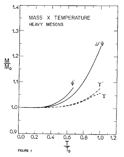
Figure 1: Mass (in vacuum mass units) plotted against temperature (in critical temperature units). $m_{c}=1640$ MeV

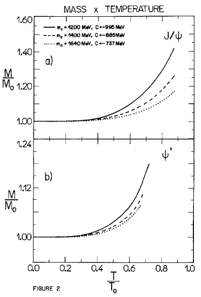
Figure 2: a) Mass (in vacuum mass units) of the charmonium groundstate as a function of temperature (in critical temperature units) for charm quark masses equal to 1200, 1400 and 1640 MeV. b) The same as a) for the charmonium first excited state.