TU-479

March, 1995

Ph.D thesis
Effects of the Gravitino on the Inflationary Universe
Takeo Moroi
Department of Physics, Tohoku University, Sendai 980-77, Japan

Chapter 1 Introduction

1.1 Overview

When we think of new physics beyond the standard model, supersymmetric (SUSY) extension [1] of the standard model is one of the most attractive candidates. Cancellation of quadratic divergences in SUSY models naturally explains the stability of the electroweak scale against radiative corrections [2, 3]. Furthermore, if we assume the particle contents of the minimal SUSY standard model (MSSM), the three gauge coupling constants in the standard model meet at $\sim 10^{16}$GeV [4, 5], which strongly supports grand unified theory (GUT) based on SUSY [6, 7].

In spite of these strong motivations, no direct evidence of SUSY (especially superpartners) has been discovered yet. Therefore, the SUSY is broken in nature, if it exists. Although many efforts have been made to understand the origin of the SUSY breaking, no convincing scenario of SUSY breaking has found yet. Nowadays, many people expect the existence of local SUSY (i.e. supergravity) [8] and try to find a mechanism to break SUSY spontaneously in the framework. In the broken phase of the supergravity, super-Higgs effect occurs and gravitino, which is the superpartner of graviton, acquires mass by absorbing the Nambu-Goldstone fermion associated with SUSY breaking. In this case, the gravitino mass $m_{3/2}$ is expected to give us some informations about the SUSY breaking mechanism. For example, in models with the minimal kinetic term, the following (tree level) super-trace formula among the mass matrices ${\bf M}_{J}^{2}$’s holds;

$${\rm Str}{\bf M}^{2}\equiv\sum_{{\rm spin}~{}J}(-1)^{2J}(2J+1){\rm tr}{\bf M}^{2}_{J}\simeq 2(n_{\phi}-1)m_{3/2}^{2},$$ (1.1)

where $n_{\phi}$ is the number of the chiral multiplets in the spontaneously broken local SUSY model. In this case, all the SUSY breaking masses of squarks and sleptons are equal to the gravitino mass at the Planck scale. Meanwhile in models with “no-scale like” Kähler potential [9, 10], SUSY breaking masses for sfermions vanish at the gravitational scale and are induced by radiative corrections, and hence the gravitino mass is not directly related to the scale of the SUSY breaking in the observable sector (which contains ordinary particles in the standard model and their superpartners). In order to understand the physics of the SUSY breaking, it is significant to clarify the property of the gravitino. But contrary to our theoretical interests, we have no hope to see the gravitino in collider experiments since its interaction is extremely weak.

On the contrary, cosmological arguments provide us some informations about the gravitino. In general, cosmology severely constrains properties of exotic particles. Let us review the constraints derived from cosmology.

• The first is on the mass density of the exotic particle during the big-bang nucleosynthesis. If it is too large, it speeds up the expansion rate of the universe during that epoch and results in too many ⁴He.

• The second is on the entropy production by the decay of the exotic particle. If the decay of the exotic particle releases a large amount of entropy, the baryon-to-photon ratio may become much well below what is observed today.

• The third arises from the effects of the decay products on the big-bang nucleosynthesis. If the photon or some charged particle is produced by the decay of the exotic particle after the big-bang nucleosynthesis has started, energetic photons induced by the decay products may destruct light nuclei (D, ³He, ⁴He) and destroy the great success of the big-bang nucleosynthesis.

• Furthermore, one can obtain the fourth constraints by considering the cosmic microwave background distortion by the exotic particle with lifetime larger than $\sim 10^{10}{\rm sec}$.

• If exotic particle is stable, its present mass density provides us a fifth constraint.

In fact, the most severe constraints on models based on supergravity are derived from the light element photo-dissociation and the present mass density of the universe.

Following the above arguments, we can obtain stringent constraints on the gravitino mass in the standard big-bang cosmology. If the gravitino is unstable, it may decay after the big-bang nucleosynthesis and releases tremendous amount of entropy, which may conflict with the big-bang nucleosynthesis scenario. As Weinberg first pointed out [11], the gravitino mass should be larger than $\sim 10{\rm TeV}$ so that the gravitino can decay before the big-bang nucleosynthesis starts. Furthermore in SUSY models with $R$-parity invariance, unstable gravitino produces heavy stable particle (i.e. the lightest superparticle) in its decay processes, which results in unacceptably high mass density of the present universe [12]. In order to reduce the number density of the lightest superparticle through pair annihilation processes, gravitinos should decay when the temperature of the universe is higher than (1 – 10)GeV. This requires that the gravitino mass should be larger than ($10^{6}$ – $10^{7}$)GeV, which seems to be disfavored from the naturalness point of view. In the case of stable gravitino, the gravitino mass larger than $\sim 1{\rm keV}$ is excluded since the present mass density of the gravitino exceeds the critical density of the present universe [13]. The above constraints on the gravitino mass seem to be very stringent especially for models with the minimal Kähler potential, since in such models the gravitino mass is expected to give the scale of the SUSY breaking in observable sector.

In the inflationary universe [14], however, situation changes [15]. In this case, the initial abundance of the gravitino is diluted during the inflation, and hence the number density of the gravitino becomes much less than that in the case of the standard big-bang cosmology. But even in the inflationary universe, the gravitino may cause the cosmological problems mentioned above since secondary gravitinos are produced through scattering processes off the background radiations or decay processes of superparticles. As we will see later, number density of the secondary gravitinos is approximately proportional to the reheating temperature after the inflation and hence the upperbound on the reheating temperature is derived.

In this thesis, we study details on the gravitino production in early universe and on its effects in the inflationary universe. Compared with the previous works, we have made an essential improvement on the following points.

• Gravitino production cross sections are calculated by using full relevant terms in the local SUSY lagrangian.

• High energy photon spectrum induced by the gravitino decay is obtained by solving the Boltzmann equations numerically.

• Time evolutions of the light nuclei (D, ³He, ⁴He) with non-standard energetic photons are calculated by modifying Kawano’s computer code.

In our analysis, we assume that the light elements are synthesized through the (almost) standard scenario of the big-bang nucleosynthesis (with baryon-to-photon ratio $10^{-9}$ – $10^{-10}$), and take the reheating temperature as a free parameter.

1.2 Organization of this thesis

The outline of this thesis is as follows. The former half of this thesis is devoted to the review of related topics, especially that of the gravitino properties. In Chapter 2, we review the motivation of SUSY. In Chapter 3, the gravitino field which is the gauge field associated with local SUSY transformation is introduced. Furthermore, lagrangian based on local SUSY is also shown in Chapter 3 and the super-trace formula in that framework is derived. Conventions used in Chapter 3 (and in other chapters) are shown in Appendix A. In Chapter 4, we quantize a massive gravitino field and derive Feynman rules for gravitino.

In the latter half of this thesis, we study the cosmology with the gravitino in detail. Overview of phenomenology with the gravitino is given in Chapter 5. In Chapter 6, effects of unstable gravitino in the inflationary cosmology are analyzed in detail. In deriving constraints, we first derive photon spectrum induced by the decay of the gravitino. The procedure to obtain the photon spectrum is given in Appendix B. Then, we calculate the time evolution of light nuclei with the obtained high energy photon spectrum, and we derive constraints on the reheating temperature and on the gravitino mass. In our analysis, we assume the standard big-bang nucleosynthesis scenario which is reviewed in Appendix C. The case of stable gravitino is discussed in Chapter 7. Chapter 8 is devoted to discussions.

Chapter 2 Motivations of supersymmetry

2.1 Hierarchy problem in the standard model

For particle physicists, symmetries in nature are significant guiding principles. Especially, interactions of elementary particles (like quarks and leptons) can be understood by using the concept of the local gauge symmetry. Strong interaction is expected to originate to ${\rm SU(3)}_{C}$ gauge group, and its theoretical predictions (like three gluon vertex and asymptotic free nature of its gauge coupling constant) have been confirmed experimentally. Meanwhile, results of recent electroweak precision measurements are in good agreements with the predictions of the spontaneously broken ${\rm SU(2)}_{L}$ $\times$ ${\rm U(1)}_{Y}$ gauge theory. Accompanied by theoretical and experimental successes, the standard model, based on the ${\rm SU(3)}_{C}$ $\times$ ${\rm SU(2)}_{L}$ $\times$ ${\rm U(1)}_{Y}$ gauge group, is regarded as the established one which describes particle interactions below the energy scale $\sim$ 100GeV.

But once we look up high energy scale, one unpleasant problem, which is called hierarchy problem, appears in the standard model. In the standard model, existence of the elementary scalar boson, i.e. Higgs boson, is assumed in order to cause a spontaneous breaking of the gauge symmetry ${\rm SU(2)}_{L}$ $\times$ ${\rm U(1)}_{Y}$ $\rightarrow$ ${\rm U(1)}_{em}$. This is the origin of the hierarchy problem. As one can easily see, radiative corrections to the Higgs boson mass squared $\delta m_{H}^{2}$ are quadratically divergent. Therefore, if one assumes the existence of the cut-off scale of the standard model $\Lambda_{CUT}$ at which the parameters in the standard model are set by a more fundamental theory, $\delta m_{H}^{2}$ $\sim$ $O(\alpha\Lambda_{CUT}^{2})$ where $\alpha$ represents the coupling factor. The relation between the bare mass squared $m_{H,B}^{2}$ and the renormalized one $m_{H,R}^{2}$ is written in the following way;

$$m_{H,R}^{2}=m_{H,B}^{2}+\delta m_{H}^{2}.$$ (2.1)

In order to give the electroweak scale correctly, the renormalized mass squared $m_{H,R}^{2}$ should be $O((100{\rm GeV})^{2})$. On the other hand, if we assume a larger value of $\Lambda_{CUT}$, $\delta m_{H}^{2}$ increases quadratically and a fine tuning of $m_{H,B}^{2}$ is needed so that the renormalized mass squared $m_{H,R}^{2}$ remains $O((100{\rm GeV})^{2})$. For example, if we assume the cut-off scale of the standard model to be at the Planck scale $\sim$ $10^{19}{\rm GeV}$, both $m_{H,B}^{2}$ and $\delta m_{H}^{2}$ are $O((10^{19}{\rm GeV})^{2})$ for $\alpha$ $\sim$ $O(1)$, and they should be chosen as

$$m_{H,B}^{2}+\delta m_{H}^{2}\sim O((10^{19}{\rm GeV})^{2})-O((10^{19}{\rm GeV})^{2})\sim O((100{\rm GeV})^{2}).$$ (2.2)

This is a terrific fine tuning. Therefore, if one assume that the cut-off scale of the standard model is much larger than the electroweak scale, we have to accept an unbelievable fine tuning of Higgs boson mass. This is the hierarchy problem. In fact, this problem stems from the fact that there is no symmetry which stabilizes the electroweak scale [16, 17]. In order to solve this problem, we hope that some new physics (in other words, some new symmetry) in which quadratic divergences do not exist at all, appears at a energy scale $O(100{\rm GeV}-1{\rm TeV})$ and solve this difficulty.

2.2 Supersymmetric extension of the standard model

One of the most attractive solution to the hierarchy problem is SUSY [1]. SUSY is a symmetry which transforms bosons into fermions and vice versa. Therefore, in SUSY models the number of bosonic degrees of freedom is equal to that of fermionic ones. As we will see later, quadratic divergence of the Higgs (and other) boson masses are canceled out between the contributions from boson and fermion loops.

Experimentally, however, we have not found any superpartners of the observed particles. This fact indicates that SUSY is broken in nature, if it exists. In order to solve the hierarchy problem, the SUSY must be broken softly [18] so that quadratic divergences do not exist at all. Usually, such a softly broken global SUSY model is regarded as a low energy effective theory of the spontaneously broken local SUSY model. We will comment on this point in the next chapter and here, we consider a phenomenologically acceptable (softly broken) SUSY model.

When we extend the standard model to the supersymmetric one, we usually add “superpartners” for the ordinary particles existed in the standard model. In Table 2.1, we show the particles in the minimal SUSY standard model (MSSM) and their gauge quantum numbers. Along with the existence of the superpartners, one big difference between the standard model and the SUSY one is the number of Higgs doublets, i.e. the MSSM requires two Higgs doublets (see Table 2.1). In the SUSY standard model, Higgs bosons are accompanied by their fermionic superpartners which have the same gauge quantum numbers as the Higgs bosons. In this case, anomaly cancellation is not guaranteed if both of $H_{1}$ and $H_{2}$ are not included. Furthermore, in order to give fermion masses to up-type quarks as well as down-type quarks and leptons from Yukawa couplings of Higgs bosons, at least two chiral superfields $H_{1}$ and $H_{2}$ are needed. Mainly from the above two reasons, two Higgs doublets with representation $({\bf 1},{\bf 2},-1/2)$ and $({\bf 1},{\bf 2},1/2)$ are introduced into the MSSM.

Gauge sector
Representation	Boson $(R=+1)$	Fermion $(R=-1)$
$({\bf 8},{\bf 1},0)$	$G_{\mu}$	$\tilde{g}$
$({\bf 1},{\bf 3},0)$	$W_{\mu}$	$\tilde{w}$
$({\bf 1},{\bf 1},0)$	$B_{\mu}$	$\tilde{b}$

Higgs sector
Representation	Boson $(R=+1)$	Fermion $(R=-1)$
$({\bf 1},{\bf 2},-1/2)$	$H_{1}$	$\chi_{H_{1}}$
$({\bf 1},{\bf 2},1/2)$	$H_{2}$	$\chi_{H_{2}}$

Quark / lepton sector
Representation	Boson $(R=-1)$	Fermion $(R=+1)$
$({\bf 3},{\bf 2},1/6)$	$\tilde{q}_{i}$	$q_{i}$
$({\bf 3^{*}},{\bf 1},-2/3)$	$\tilde{u}^{c}_{i}$	$u^{c}_{i}$
$({\bf 3^{*}},{\bf 1},1/3)$	$\tilde{d}^{c}_{i}$	$d^{c}_{i}$
$({\bf 1},{\bf 2},-1/2)$	$\tilde{l}_{i}$	$l_{i}$
$({\bf 1},{\bf 2},1)$	$\tilde{e}^{c}_{i}$	$e^{c}_{i}$

Table 2.1: Particle content of the minimal SUSY standard model. Index $i$ is the generation index which runs from 1 to 3. For each particles, representation of the ${\rm SU(3)}_{C}$ $\times$ ${\rm SU(2)}_{L}$ $\times$ ${\rm U(1)}_{Y}$ gauge group is also shown.

Next, we will see the lagrangian of the MSSM. As a first step, we comment on $R$-parity. If we assume a particle content of the MSSM shown in Table 2.1, we can write down interactions which violate baryon- or lepton-number conservations. For example, interactions such as $u^{c}d^{c}\tilde{d}^{c}$ or $d^{c}q\tilde{l}$ cannot be forbidden by gauge invariance or renormalizability. But phenomenologically, strength of these interactions is severely constrained since they may induce unwantedly high rate of nucleon decay and neutron-anti-neutron oscillation, and they wash out baryon number in the early universe [19]. Rather than assuming extremely small coupling constants for them, we usually forbid these dangerous terms by introducing a discrete symmetry, that is called $R$-parity. $R$-parity assigns $+1$ for ordinary particles in the standard model and $-1$ for their superpartners. One can see that if we require the invariance under the $R$-parity, baryon- and lepton-numbers are conserved under the restriction of renormalizability. In this thesis, we adopt the $R$-invariance below. Notice that $R$-invariance also guarantees the stability of the lightest $R$-odd particle, i.e. the lightest superparticle (LSP).

Assuming the $R$-invariance, the superpotential of the MSSM is given by

$$W_{\rm MSSM} = y^{(u)}_{ij}u^{c}_{i}q_{j}H_{2}+y^{(d)}_{ij}d^{c}_{i}q_{j}H_{1}+y^{(e)}_{ij}e^{c}_{i}l_{j}H_{1}$$ (2.3)

$$+\mu_{H}H_{1}H_{2},$$

where $i$ and $j$ are generation indices, and we have omitted the group indices for simplicity. Here, $y^{(u)}$, $y^{(d)}$ and $y^{(e)}$ are the Yukawa coupling constants of the up-, down- and lepton-sector, respectively.

Since the SUSY should be broken in nature, SUSY breaking terms are also necessary in lagrangian. In order not to induce quadratic divergences, SUSY should be broken softly. In general, soft SUSY breaking terms are gaugino mass terms, scalar mass terms and trilinear coupling terms for scalar bosons of same chirality [18]. In the MSSM, SUSY breaking terms are given by

$${\cal L}_{\rm soft} = -m^{2}_{\tilde{q}ij}\tilde{q}^{*}_{i}\tilde{q}_{j}-m^{2}_{\tilde{u}ij}\tilde{u}^{c*}_{i}\tilde{u}^{c}_{j}-m^{2}_{\tilde{d}ij}\tilde{d}^{c*}_{i}\tilde{d}^{c}_{j}-m^{2}_{\tilde{l}ij}\tilde{l}^{*}_{i}\tilde{l}_{j}-m^{2}_{\tilde{e}ij}\tilde{e}^{c*}_{i}\tilde{e}^{c}_{j}$$ (2.4)

$$-\left(A^{(u)}_{ij}\tilde{u}^{c}_{i}\tilde{q}_{j}H_{2}+A^{(d)}_{ij}\tilde{d}^{c}_{i}\tilde{q}_{j}H_{1}+A^{(e)}_{ij}\tilde{e}^{c}_{i}\tilde{l}_{j}H_{1}+h.c.\right)$$

$$-m_{H_{1}}^{2}\left|H_{1}\right|^{2}-m_{H_{2}}^{2}\left|H_{2}\right|^{2}-\left(m_{3}^{2}H_{1}H_{2}+h.c.\right)$$

$$-\left(m_{G3}\tilde{g}\tilde{g}+m_{G2}\tilde{w}\tilde{w}+m_{G1}\tilde{b}\tilde{b}+h.c.\right),$$

where $m^{2}_{\tilde{q}}$ – $m^{2}_{\tilde{e}}$ are the squark and slepton masses, and $m_{G3}$ – $m_{G1}$ the gauge fermion masses. In the next chapter, we will see that these SUSY breaking parameters can be obtained in a low energy effective theory of local SUSY models.

Figure 2.1: Quadratically divergent Feynman diagrams for the $H_{2}$ mass. Diagram with CF (CB, GB, GF) is the contribution from chiral fermion (chiral boson, gauge boson, gauge fermion) loop. Dashed lines in external lines represent $H_{2}$. Notice that the diagram with $H_{2}$ loop (lower-left) originates to the gauge $D$-term, and hence we classify it as the contribution of gauge boson.

As mentioned before, quadratic divergence of the two point functions of scalar bosons disappears in SUSY models. At the one loop level, this can be easily seen. For example, we will see the cancellation in the mass of $H_{2}$. Feynman diagrams which give quadratically divergent radiative corrections to the $H_{2}$ mass are shown in Fig. 2.1. Each of them are quadratically divergent;

$$\left.\delta m_{H_{2}}^{2}\right|_{\rm CB} \simeq \frac{1}{8\pi^{2}}y^{(u)}_{ij}y^{(u)*}_{ij}\Lambda_{CUT}^{2}+\cdot\cdot\cdot,$$ (2.5)

$$\left.\delta m_{H_{2}}^{2}\right|_{\rm CF} \simeq -\frac{1}{8\pi^{2}}y^{(u)}_{ij}y^{(u)*}_{ij}\Lambda_{CUT}^{2}+\cdot\cdot\cdot,$$ (2.6)

$$\left.\delta m_{H_{2}}^{2}\right|_{\rm GB} \simeq \frac{1}{4\pi^{2}}\left(\frac{1}{2}g_{2}^{2}+\frac{1}{4}g_{1}^{2}\right)\Lambda_{CUT}^{2}+\cdot\cdot\cdot,$$ (2.7)

$$\left.\delta m_{H_{2}}^{2}\right|_{\rm GF} \simeq -\frac{1}{4\pi^{2}}\left(\frac{1}{2}g_{2}^{2}+\frac{1}{4}g_{1}^{2}\right)\Lambda_{CUT}^{2}+\cdot\cdot\cdot,$$ (2.8)

where CF (CB, GB, GF) represents the contribution from chiral fermion (chiral boson, gauge boson, gauge fermion), $\cdot\cdot\cdot$ the terms which do not contain quadratic divergences and $\Lambda_{CUT}$ the cut-off. These quadratic divergences, however, cancel out between boson and fermion loops. Quadratic divergences in other scalar masses also disappear in the same way, and hence the hierarchy problem can be solved by extending the standard model to the supersymmetric one.

In the MSSM, other interesting new physics, i.e. the grand unified theory (GUT) [20], is suggested from the renormalization group analysis [4, 5]. As mentioned before, SUSY extension of the standard model increases the number of particles, which changes the renormalization group equation of the gauge coupling constants. In Fig. 2.2, we show the renormalization group flow of ${\rm SU(3)}_{C}$, ${\rm SU(2)}_{L}$ and ${\rm U(1)}_{Y}$ gauge coupling constants in the MSSM case and in the standard model case. In the MSSM case, three gauge coupling constants meet at the energy scale $\sim 10^{16}{\rm GeV}$ which may be identified with the GUT scale, while in the standard model case, the renormalization group flow of the gauge coupling constants conflicts with the gauge coupling unification.

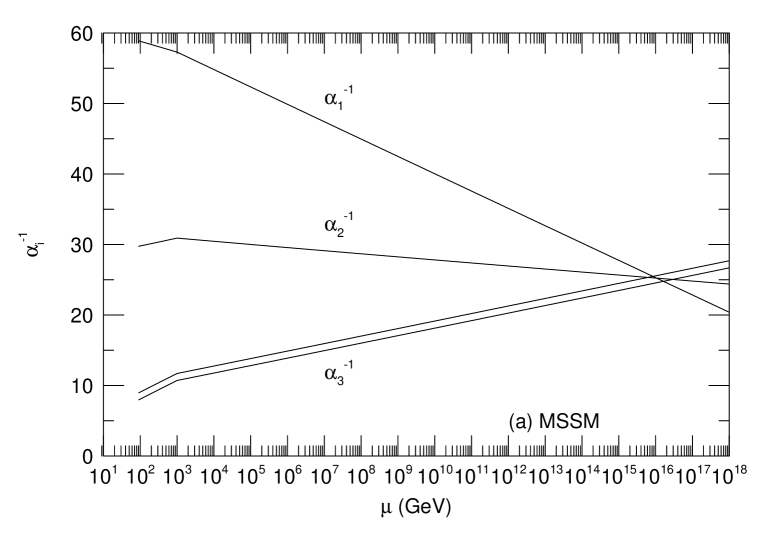
Figure 2.2: Renormalization group flow of the coupling constants of ${\rm SU(3)}_{C}$, ${\rm SU(2)}_{L}$ and ${\rm U(1)}_{Y}$ gauge group for the case of (a) the MSSM, and (b) the standard model. Here, we use two loop renormalization group equations, and take the SUSY scale at 1TeV for the MSSM case.

Another indirect evidence of SUSY GUT is the bottom-tau mass ratio [21, 22, 23]. In SU(5) or SO(10) GUT, Yukawa coupling constants of down- and lepton-sectors to the Higgs boson are also expected to be unified at the GUT scale, and hence we can get a relation between the bottom- and tau-Yukawa coupling constants at the electroweak scale. By using this relation, the mass of the bottom quark is obtained once the tau-lepton mass ($\simeq 1.777{\rm GeV}$ [24]) is fixed. In Fig. 2.3, we show the predicted bottom-quark mass as a function of $\tan\beta=\left\langle{H_{1}}\right\rangle/\left\langle{H_{2}}\right\rangle$. Notice that the maximal and minimal values for $\tan\beta$ are determined so that all the Yukawa coupling constants do not blow up below the GUT scale. As one can see, SUSY GUT predicts the bottom-quark mass to be (4 – 6)GeV which is close to that determined from experiments; $m_{b}(m_{b})=(4.25\pm 0.2){\rm GeV}$ [25] (where we have doubled the uncertainty), especially when $\tan\beta$ approaches its maximal or minimal value.

Figure 2.3: The predicted value of the running bottom-quark mass $m_{b}(m_{b})$ is shown as a function of $\tan\beta$ for $\alpha_{3}(m_{Z})=0.11$ and 0.12. Here, we take the (on-shell) top-quark mass at 174GeV.

Contrary to those attractive features, no direct evidence of SUSY has been found, which certainly indicates that the SUSY is a (softly) broken symmetry. The physics of SUSY breaking is, however, still an open question and we have not understood it yet. Especially in the framework of global SUSY, it seems to be very much difficult to construct a phenomenologically favorable model. One of the reason is that there exists a mass formula in the global SUSY model;

$${\rm Str}{\bf M}^{2}\equiv\sum_{J=0}^{1}(-1)^{J}{\rm tr}{\bf M}_{J}^{2}=0,$$ (2.9)

which prevents all the squarks and sleptons from having masses larger than those of quarks and leptons. To avoid this constraint, many people extend the global SUSY to the local one and consider the physics of SUSY breaking in the framework of supergravity. In the next chapter, we will investigate local SUSY model and see how the mass formula in global SUSY models (2.9) is modified.

Chapter 3 Review of supergravity

In this chapter, we will introduce a lagrangian which is invariant under the local SUSY transformation, and derive super-trace formula in that framework. Conventions used in this chapter are essentially equal to those used in ref.[26] except that we use the metric (in flat space-time) as $g_{\mu\nu}\simeq{\rm diag}(1,-1,-1,-1)$. For our convention, see also Appendix A.

3.1 Heuristic approach to supergravity lagrangian

Compared with the global SUSY, one of the characteristics of the local one is the existence of a gauge field associated with the local SUSY, which is called gravitino. As in the case of ordinary gauge theories, the gravitino couples to a Noether current of SUSY and maintains the invariance under the local SUSY transformation. In this section, we will briefly review the role of the gravitino in the local SUSY theory by using the simplest model, which is the Wess-Zumino model [1] without interactions.

Let us begin with the global case. In this case, total lagrangian contains only two terms, one is the kinetic term of a massless complex scalar boson $\phi$ and the other is that of a massless chiral fermion $\chi$;

$${\cal L}_{\rm WZ}=\partial^{\mu}\phi\partial_{\mu}\phi^{*}+i\overline{\chi}\bar{\sigma}^{\mu}\partial_{\mu}\chi.$$ (3.1)

Up to total derivative, this lagrangian is invariant under the following global SUSY transformation,

$$\delta\phi = \sqrt{2}\xi\chi,$$ (3.2)

$$\delta\chi = -i\sqrt{2}\sigma^{\mu}\overline{\xi}(\partial_{\mu}\phi),$$ (3.3)

where $\xi$ is the infinitesimal Grassmann-odd parameter.

If $\xi$ has space-time dependence, lagrangian (3.1) is not invariant but extra terms which are proportional to $\partial\xi$ or $\partial\overline{\xi}$ appear with the supertransformation (3.2) and (3.3);

$$\delta{\cal L}_{\rm WZ} = \sqrt{2}\left\{(\partial_{\mu}\xi)\sigma^{\nu}\bar{\sigma}^{\mu}\chi(\partial_{\nu}\phi^{*})+\overline{\chi}\bar{\sigma}^{\mu}\sigma^{\nu}(\partial_{\mu}\overline{\xi})(\partial_{\nu}\phi)\right\}+({\rm total~{}derivative})$$ (3.4)

$$\equiv i(\partial_{\mu}\xi)J^{\mu}+h.c.+({\rm total~{}derivative}).$$

where

$$J^{\mu}\equiv-i\sqrt{2}\sigma^{\nu}\bar{\sigma}^{\mu}\chi(\partial_{\nu}\phi^{*}).$$ (3.5)

Notice that $J^{\mu}$ is the Noether current of SUSY, which is called supercurrent. In order to keep invariance, we introduce a gauge field $\psi_{\mu}$. As in the cases of ordinary gauge theories, the gauge field $\psi_{\mu}$ couples to the supercurrent in the following way;

$${\cal L}_{\psi J}=-\frac{i}{2}G_{S}\psi_{\mu}J^{\mu}+h.c.~{},$$ (3.6)

where $G_{S}$ is the “coupling constant” which we will determine later. Since the charge of SUSY has a Grassmann-odd nature with spin index, the gauge field $\psi_{\mu}$ associated with SUSY is a spin $\frac{3}{2}$ fermion. Varying eq.(3.6), one obtains

$$\delta{\cal L}_{\psi J}=-\frac{i}{2}G_{S}\left\{(\delta\psi_{\mu})J^{\mu}+\psi_{\mu}(\delta J^{\mu})\right\}+h.c.$$ (3.7)

Therefore, if $\psi_{\mu}$ transforms as

$$\delta\psi_{\mu}\sim\frac{2}{G_{S}}\partial_{\mu}\xi,$$ (3.8)

the first term in eq.(3.7) cancels out the contribution from eq.(3.4).

Next, we will consider the second term in eq.(3.7). Supertransformation of the supercurrent (3.5) gives energy-momentum tensor ${T_{\mu}}^{\nu}$ of the chiral multiplet $(\phi,\chi)$;

$$\left\{\overline{Q}_{\dot{\alpha}},J^{\mu}_{\alpha}\right\} = -2\sigma^{\nu}_{\alpha\dot{\alpha}}{T_{\nu}}^{\mu}+({\rm total~{}derivative}),$$

$$\left\{Q^{\alpha},\overline{J}^{\mu\dot{\alpha}}\right\} = -2\bar{\sigma}^{\nu\dot{\alpha}\alpha}{T_{\nu}}^{\mu}+({\rm total~{}derivative}),$$ (3.9)

where $Q$ and $\overline{Q}$ are the generators of the SUSY transformation, and hence the second term in eq.(3.7) becomes

$$-\frac{i}{2}G_{S}\left\{\psi_{\mu}(\delta J^{\mu})\right\}+h.c.=\frac{i}{2}G_{S}\left\{\psi_{\mu}\sigma_{\nu}\overline{\xi}+\psi_{\nu}\sigma_{\mu}\overline{\xi}+\overline{\psi}_{\mu}\bar{\sigma}_{\nu}\xi+\overline{\psi}_{\nu}\bar{\sigma}_{\mu}\xi\right\}T^{\mu\nu}.$$ (3.10)

In order to cancel out these terms, we rewrite the lagrangian (3.1) by explicitly expressing the metric tensor $g_{\mu\nu}$;

$${\cal L}_{\rm WZ}\rightarrow\sqrt{-g}g_{\mu\nu}\left(\partial^{\mu}\phi\partial^{\nu}\phi^{*}+i\overline{\chi}\bar{\sigma}^{\mu}\partial^{\nu}\chi\right),$$ (3.11)

where $g\equiv\det{g_{\mu\nu}}$, and use the fact that the metric is the gauge field associated with the energy-momentum tensor (which is the Noether current of the space-time translation), that is, the energy-momentum tensor ${T_{\mu}}^{\nu}$ is obtained if one varies lagrangian by $g_{\mu\nu}$;

$$\frac{\partial{\cal L}}{\partial g_{\mu\nu}}\sim 2T^{\mu\nu}.$$ (3.12)

Then, the metric tensor $g_{\mu\nu}$ (i.e. graviton) can be regarded as a superpartner of the gravitino field $\psi_{\mu}$, and its transformation law is determined so that the local SUSY invariance is maintained;

$$\delta g_{\mu\nu}\frac{\delta{\cal L}_{\rm WZ}}{\delta g_{\mu\nu}}\sim-\frac{i}{2}G_{S}\left\{\psi^{\mu}\sigma^{\nu}\overline{\xi}+\psi^{\nu}\sigma^{\mu}\overline{\xi}+\overline{\psi}^{\mu}\bar{\sigma}^{\nu}\xi+\overline{\psi}^{\nu}\bar{\sigma}^{\mu}\xi\right\}T_{\mu\nu}.$$ (3.13)

Combining eq.(3.12) with eq.(3.13), one can obtain the transformation law of the metric tensor;

$$\delta g_{\mu\nu}\sim-iG_{S}\left(\psi_{\mu}\sigma_{\nu}\overline{\xi}+\psi_{\nu}\sigma_{\mu}\overline{\xi}+\overline{\psi}_{\mu}\bar{\sigma}_{\nu}\xi+\overline{\psi}_{\nu}\bar{\sigma}_{\mu}\xi\right).$$ (3.14)

In the following arguments, in fact, it is more convenient to use the vierbein ${e_{\mu}}^{a}$ rather than the metric tensor $g_{\mu\nu}=\eta_{ab}{e_{\mu}}^{a}{e_{\nu}}^{b}$, where $\eta_{ab}={\rm diag}(1,-1,-1,-1)$ is the metric tensor in flat space-time. In supergravity models, transformation law of the vierbein ${e_{\mu}}^{a}$ is defined as

$$\delta{e_{\mu}}^{a}=-iG_{S}\left(\xi\sigma^{a}\overline{\psi}_{\mu}+\overline{\xi}\bar{\sigma}^{a}\psi_{\mu}\right),$$ (3.15)

with $G_{S}=M^{-1}$. This transformation law gives eq.(3.14). Under the local SUSY transformation, the vierbein ${e_{\mu}}^{a}$ and the gravitino $\psi_{\mu}$ (and some other auxiliary fields) make up a multiplet, which we call a supergravity multiplet.

As we have seen, if we extend the global SUSY to the local one, the metric tensor $g_{\mu\nu}$ automatically comes into the theory, and hence we must consider gravity. This is the reason why the local SUSY is sometimes called supergravity.

3.2 Minimal supergravity model

In the previous section, we have introduced the gravitino field $\psi_{\mu}$ in order to keep the local SUSY invariance. As we have seen, the gravitino field couples to the supercurrent, but the strength $G_{S}$ of the coupling between the gravitino and the supercurrent has not been determined yet. In order to determine the coupling strength $G_{S}$, we must see the invariance of the kinetic terms of ${e_{\mu}}^{a}$ and $\psi_{\mu}$ under the local SUSY transformation.

In this section, we will explicitly investigate the local SUSY invariance of the minimal supergravity model which contains only the graviton ${e_{\mu}}^{a}$ and the gravitino field $\psi_{\mu}$. As a result, we will see the coupling strength $G_{S}$ should be equal to the inverse of the gravitational scale.

The lagrangian of the minimal supergravity model is given by

$${\cal L}_{\rm MSG}={\cal L}_{\rm EH}+{\cal L}_{\rm RS},$$ (3.16)

where ${\cal L}_{\rm EH}$ is the usual Einstein-Hilbert lagrangian, and ${\cal L}_{\rm RS}$ is the Rarita-Schwinger lagrangian which is essentially the kinetic term of the spin $\frac{3}{2}$ gravitino field. The Einstein-Hilbert lagrangian is given by

$${\cal L}_{\rm EH}=-\frac{M^{2}}{2}eR,$$ (3.17)

with

$$R\equiv{e_{a}}^{\mu}{e_{b}}^{\nu}\left(\partial_{\mu}{\omega_{\nu}}^{ab}-\partial_{\nu}{\omega_{\mu}}^{ab}-{\omega_{\mu}}^{ac}{\omega_{\nu c}}^{b}+{\omega_{\nu}}^{ac}{\omega_{\mu c}}^{b}\right),$$ (3.18)

where ${\omega_{\mu}}^{ab}$ denotes the spin connection and $e\equiv\det{e_{a}}^{\mu}$. On the other hand, the Rarita-Schwinger lagrangian can be written as

$${\cal L}_{\rm RS}=e\epsilon^{\mu\nu\rho\sigma}\overline{\psi}_{\mu}\bar{\sigma}_{\nu}\tilde{{\cal D}}_{\rho}\psi_{\sigma},$$ (3.19)

where $\epsilon^{\mu\nu\rho\sigma}$ is the totally anti-symmetric tensor ($\epsilon_{0123}=-1$ in flat space-time) and the covariant derivative of the gravitino field is given by

$$\tilde{\cal D}_{\mu}\psi_{\nu}\equiv\partial_{\mu}\psi_{\nu}+\frac{1}{2}{\omega_{\mu}}^{ab}\sigma_{ab}\psi_{\nu}.$$ (3.20)

In the following, we will see the invariance of the minimal supergravity lagrangian (3.16) under the local SUSY transformation;

$$\delta{e_{\mu}}^{a}=-iG_{S}\left(\xi\sigma^{a}\overline{\psi}_{\mu}+\overline{\xi}\bar{\sigma}^{a}\psi_{\mu}\right),$$ (3.21)

$$\delta\psi_{\mu}=\frac{2}{G_{S}}\tilde{\cal D}_{\mu}\xi\equiv\frac{2}{G_{S}}\left(\partial_{\mu}\xi+\frac{1}{2}{\omega_{\mu}}^{ab}\sigma_{ab}\xi\right),$$ (3.22)

where parameter $G_{S}$ will be determined so that the local SUSY invariance is maintained (see eq.(3.8) and eq.(3.15)).

Before checking the invariance of the minimal supergravity lagrangian (3.16), we will comment on the spin connection ${\omega_{\mu}}^{ab}$. As we will see below, ${\omega_{\mu}}^{ab}$ is represented as a function of the vierbein ${e_{\mu}}^{a}$ and the gravitino $\psi_{\mu}$ by solving its field equation;

$$\frac{\delta{\cal L}_{\rm MSG}}{\delta{\omega_{\mu}}^{ab}}=\frac{\partial{\cal L}_{\rm MSG}}{\partial{\omega_{\mu}}^{ab}}-\partial_{\nu}\frac{\partial{\cal L}_{\rm MSG}}{\partial\left(\partial_{\nu}{\omega_{\mu}}^{ab}\right)}=0,$$ (3.23)

and hence ${\omega_{\mu}}^{ab}$ is regarded as an auxiliary field. From eq.(3.23), one can obtain

$$M^{2}\left\{\left(\partial_{\mu}{e_{\nu}}^{a}+{\omega_{\mu}}^{ab}e_{\nu b}\right)-\left(\partial_{\nu}{e_{\mu}}^{a}+{\omega_{\nu}}^{ab}e_{\mu b}\right)\right\}=-\frac{i}{2}\left(\overline{\psi}_{\mu}\bar{\sigma}^{a}\psi_{\nu}-\overline{\psi}_{\nu}\bar{\sigma}^{a}\psi_{\mu}\right).$$ (3.24)

By solving this equation, explicit form of the spin connection is given by

$$\omega_{\mu\rho\sigma} \equiv e_{\rho a}e_{\sigma b}{\omega_{\mu}}^{ab}$$ (3.25)

$$= \frac{1}{2}\left\{e_{\sigma a}\left(\partial_{\mu}{e_{\rho}}^{a}-\partial_{\rho}{e_{\mu}}^{a}\right)+e_{\rho a}\left(\partial_{\sigma}{e_{\mu}}^{a}-\partial_{\mu}{e_{\sigma}}^{a}\right)-e_{\mu a}\left(\partial_{\rho}{e_{\sigma}}^{a}-\partial_{\sigma}{e_{\rho}}^{a}\right)\right\}$$

$$-\frac{i}{4M^{2}}e_{\sigma a}\left(\psi_{\rho}\sigma^{a}\overline{\psi}_{\mu}-\psi_{\mu}\sigma^{a}\overline{\psi}_{\rho}\right)-\frac{i}{4M^{2}}e_{\rho a}\left(\psi_{\mu}\sigma^{a}\overline{\psi}_{\sigma}-\psi_{\sigma}\sigma^{a}\overline{\psi}_{\mu}\right)$$

$$+\frac{i}{4M^{2}}e_{\mu a}\left(\psi_{\sigma}\sigma^{a}\overline{\psi}_{\rho}-\psi_{\rho}\sigma^{a}\overline{\psi}_{\sigma}\right).$$

Now let us see the invariance of the lagrangian (3.16). With the help of chain rule, variation of the total lagrangian is given by

$$\delta{\cal L}_{\rm MSG} = \delta{e_{\mu}}^{a}\left.\frac{\delta{\cal L}_{\rm MSG}}{\delta{e_{\mu}}^{a}}\right|_{\psi,\omega}+\delta\psi_{\mu}\left.\frac{\delta{\cal L}_{\rm MSG}}{\delta\psi_{\mu}}\right|_{e,\omega}$$ (3.26)

$$+\left(\delta{e_{\mu}}^{a}\frac{\delta{\omega_{\mu}}^{ab}}{\delta{e_{\mu}}^{a}}+\delta\psi_{\mu}\frac{\delta{\omega_{\mu}}^{ab}}{\delta\psi_{\mu}}\right)\left.\frac{\delta{\cal L}_{\rm MSG}}{\delta{\omega_{\mu}}^{ab}}\right|_{e,\psi}~{},$$

where we have used the fact that the spin connection ${\omega_{\mu}}^{ab}$ is a function of the vierbein ${e_{\mu}}^{a}$ and the gravitino $\psi_{\mu}$. The important point is that the last two terms in eq.(3.26) which are proportional to $(\delta{\cal L}_{\rm MSG}/\delta\omega)$ vanish since the spin connection obeys its field equation $(\delta{\cal L}_{\rm MSG}/\delta\omega)=0$. Therefore, we only have to vary ${e_{\mu}}^{a}$ and $\psi_{\mu}$ (with ${\omega_{\mu}}^{ab}$ fixed) in order to obtain $\delta{\cal L}_{\rm MSG}$. (We denote this operation $\Delta$.)

Variation of the Einstein-Hilbert lagrangian ${\cal L}_{\rm EH}$ gives the Einstein tensor multiplied by $\delta{e_{\mu}}^{a}$;

$$\Delta{\cal L}_{\rm EH} \equiv \delta{e_{\mu}}^{a}\left.\frac{\delta{\cal L}_{\rm EH}}{\delta{e_{\mu}}^{a}}\right|_{\psi,\omega}+\delta\psi_{\mu}\left.\frac{\delta{\cal L}_{\rm EH}}{\delta\psi_{\mu}}\right|_{e,\omega}$$ (3.27)

$$= iG_{S}M^{2}e\left({R_{a}}^{\mu}-\frac{1}{2}{e_{a}}^{\mu}R\right)\overline{\psi}_{\mu}\sigma^{a}\xi+h.c.~{},$$

with

$${R_{\mu}}^{a}\equiv{e_{b}}^{\nu}\left(\partial_{\mu}{\omega_{\nu}}^{ab}-\partial_{\nu}{\omega_{\mu}}^{ab}-{\omega_{\mu}}^{ac}{\omega_{\nu c}}^{b}+{\omega_{\nu}}^{ac}{\omega_{\mu c}}^{b}\right).$$ (3.28)

On the other hand, after some straightforward calculations, $\Delta{\cal L}_{\rm RS}$ becomes the following form;

$$\Delta{\cal L}_{\rm RS} \equiv \delta{e_{\mu}}^{a}\left.\frac{\delta{\cal L}_{\rm RS}}{\delta{e_{\mu}}^{a}}\right|_{\psi,\omega}+\delta\psi_{\mu}\left.\frac{\delta{\cal L}_{\rm RS}}{\delta\psi_{\mu}}\right|_{e,\omega}$$ (3.29)

$$= \left\{-\frac{i}{G_{S}}M^{2}e\left({R_{a}}^{\mu}-\frac{1}{2}{e_{a}}^{\mu}R\right)\overline{\psi}_{\mu}\bar{\sigma}^{a}\xi+h.c.\right\}$$

$$-e\epsilon^{\mu\nu\rho\sigma}\left\{\frac{2}{G_{S}}\left(\partial_{\mu}{e_{\nu}}^{a}+{\omega_{\mu}}^{ab}e_{\nu b}\right)+iG_{S}\left(\overline{\psi}_{\mu}\bar{\sigma}^{a}\psi_{\nu}\right)\right\}\overline{\xi}\bar{\sigma}_{a}\tilde{\cal D}_{\rho}\psi_{\sigma}.$$

By setting $G_{S}=M^{-1}$, the first line in eq.(3.29) is equal to $-\Delta{\cal L}_{\rm EH}$, the second line vanishes due to eq.(3.24), and hence $\delta{\cal L}_{\rm MSG}$ vanishes;

$$\delta{\cal L}_{\rm MSG}=\Delta{\cal L}_{\rm EH}+\Delta{\cal L}_{\rm RS}=0.$$ (3.30)

This is the end of the proof of the invariance. We have seen the invariance of the minimal supergravity lagrangian (3.16) under the local SUSY transformation (3.21) and (3.22) with $G_{S}=M^{-1}$.

This fact suggests that the coupling strength $G_{S}$ between the gravitino field $\psi_{\mu}$ and the supercurrent $J_{\mu}$ is not a free parameter but a model independent constant which is determined by the requirement that the kinetic term of the supergravity multiplet ($\psi_{\mu}$, ${e_{\mu}}^{a}$) is invariant under the local SUSY transformation. In the next section, we can see that general supergravity lagrangian contains interaction terms between the gravitino field $\psi_{\mu}$ and the supercurrent $J_{\mu}$ with definite coupling strength (i.e. $G_{S}=M^{-1}$);

$${\cal L}_{\psi J}=-\frac{i}{2M}\psi_{\mu}J^{\mu}+h.c.$$ (3.31)

As we will see in the following chapters, such interaction terms become very important in investigating phenomenology with the gravitino.

3.3 General supergravity lagrangian

In this section, we will extend the minimal supergravity model to general one. Derivation of the general supergravity lagrangian is given in elsewhere [8, 26], but it is very much complicated task. Therefore, we only give a final form here by following ref.[26]. In this section, we use the $M=1$ unit for simplicity.

The general supergravity lagrangian is essentially characterized by three functions; Kähler potential $K(\phi,\phi^{*})$, superpotential $W(\phi)$, and kinetic function $f(\phi)$ for vector multiplets. Notice that the Kähler potential $K(\phi,\phi^{*})$ is a function of scalar fields $\phi$ and $\phi^{*}$, while the superpotential $W(\phi)$ and the kinetic function $f(\phi)$ depend scalar fields with definite chirality.

By using these functions, the general form of the supergravity lagrangian, which contains scalar field $\phi$, chiral fermion $\chi$, gauge boson $A_{\mu}$, and gauge fermion $\lambda$ as well as the vierbein ${e_{\mu}}^{a}$ and the gravitino $\psi_{\mu}$ can be written as

$${\cal L}_{\rm SUGRA} = -\frac{1}{2}eR+eg_{ij^{*}}\tilde{\cal D}_{\mu}\phi^{i}\tilde{\cal D}^{\mu}\phi^{*j}-\frac{1}{2}eg^{2}D_{(a)}D^{(a)}$$ (3.32)

$$+ieg_{ij^{*}}\overline{\chi}^{j}\bar{\sigma}^{\mu}\tilde{\cal D}_{\mu}\chi^{i}+e\epsilon^{\mu\nu\rho\sigma}\overline{\psi}_{\mu}\bar{\sigma}_{\nu}\tilde{{\cal D}}_{\rho}\psi_{\sigma}$$

$$-\frac{1}{4}ef^{R}_{(ab)}F_{\mu\nu}^{(a)}F^{\mu\nu(b)}+\frac{1}{8}e\epsilon^{\mu\nu\rho\sigma}f^{I}_{(ab)}F_{\mu\nu}^{(a)}F_{\rho\sigma}^{(b)}$$

$$+\frac{i}{2}e\left[\lambda_{(a)}\sigma^{\mu}\tilde{\cal D}_{\mu}\overline{\lambda}^{(a)}+\overline{\lambda}_{(a)}\bar{\sigma}^{\mu}\tilde{\cal D}_{\mu}\lambda^{(a)}\right]-\frac{1}{2}f^{I}_{(ab)}\tilde{\cal D}_{\mu}\left[e\lambda^{(a)}\sigma^{\mu}\overline{\lambda}^{(b)}\right]$$

$$+\sqrt{2}egg_{ij^{*}}X^{*j}_{(a)}\chi^{i}\lambda^{(a)}+\sqrt{2}egg_{ij^{*}}X^{i}_{(a)}\overline{\chi}^{j}\overline{\lambda}^{(a)}$$

$$-\frac{i}{4}\sqrt{2}eg\partial_{i}f_{(ab)}D^{(a)}\chi^{i}\lambda^{(b)}+\frac{i}{4}\sqrt{2}eg\partial_{i^{*}}f^{*}_{(ab)}D^{(a)}\overline{\chi}^{i}\overline{\lambda}^{(b)}$$

$$-\frac{1}{4}\sqrt{2}e\partial_{i}f_{(ab)}\chi^{i}\sigma^{\mu\nu}\lambda^{(a)}F_{\mu\nu}^{(b)}-\frac{1}{4}\sqrt{2}e\partial_{i^{*}}f^{*}_{(ab)}\overline{\chi}^{i}\bar{\sigma}^{\mu\nu}\overline{\lambda}^{(a)}F_{\mu\nu}^{(b)}$$

$$+\frac{1}{2}egD_{(a)}\psi_{\mu}\sigma^{\mu}\overline{\lambda}^{(a)}-\frac{1}{2}egD_{(a)}\overline{\psi}_{\mu}\bar{\sigma}^{\mu}\lambda^{(a)}$$

$$-\frac{1}{2}\sqrt{2}eg_{ij^{*}}\tilde{\cal D}_{\nu}\phi^{*j}\chi^{i}\sigma^{\mu}\bar{\sigma}^{\nu}\psi_{\mu}-\frac{1}{2}\sqrt{2}eg_{ij^{*}}\tilde{\cal D}_{\nu}\phi^{i}\overline{\chi}^{j}\bar{\sigma}^{\mu}\sigma^{\nu}\overline{\psi}_{\mu}$$

$$-\frac{i}{4}e\left[\psi_{\mu}\sigma^{\nu\rho}\sigma^{\mu}\overline{\lambda}_{(a)}+\overline{\psi}_{\mu}\bar{\sigma}^{\nu\rho}\bar{\sigma}^{\mu}\lambda_{(a)}\right]\left[F_{\nu\rho}^{(a)}+\hat{F}_{\nu\rho}^{(a)}\right]$$

$$+\frac{1}{4}eg_{ij^{*}}\left[i\epsilon^{\mu\nu\rho\sigma}\psi_{\mu}\sigma_{\nu}\overline{\psi}_{\rho}+\psi_{\mu}\sigma^{\sigma}\overline{\psi}^{\mu}\right]\chi^{i}\sigma_{\sigma}\overline{\chi}^{i}$$

$$-\frac{1}{8}e\left[g_{ij^{*}}g_{kl^{*}}-2R_{ij^{*}kl^{*}}\right]\chi^{i}\chi^{k}\overline{\chi}^{j}\overline{\chi}^{l}$$

$$+\frac{1}{16}e\left[2g_{ij^{*}}f^{R}_{(ab)}+f^{R(cd)-1}\partial_{i}f_{(bc)}\partial_{j^{*}}f^{*}_{(ad)}\right]\overline{\chi}^{j}\bar{\sigma}^{\mu}\chi^{i}\overline{\lambda}^{(a)}\bar{\sigma}_{\mu}\lambda^{(b)}$$

$$+\frac{1}{8}e\nabla_{i}\partial_{j}f_{(ab)}\chi^{i}\chi^{j}\lambda^{(a)}\lambda^{(b)}+\frac{1}{8}e\nabla_{i^{*}}\partial_{j^{*}}f^{*}_{(ab)}\overline{\chi}^{i}\overline{\chi}^{j}\overline{\lambda}^{(a)}\overline{\lambda}^{(b)}$$

$$+\frac{1}{16}ef^{R(cd)-1}\partial_{i}f_{(ac)}\partial_{j}f_{(bd)}\chi^{i}\lambda^{(a)}\chi^{j}\lambda^{(b)}$$

$$+\frac{1}{16}ef^{R(cd)-1}\partial_{i^{*}}f^{*}_{(ac)}\partial_{j^{*}}f^{*}_{(bd)}\overline{\chi}^{i}\overline{\lambda}^{(a)}\overline{\chi}^{j}\overline{\lambda}^{(b)}$$

$$-\frac{1}{16}eg^{ij^{*}}\partial_{i}f_{(ab)}\partial_{j^{*}}f^{*}_{(cd)}\lambda^{(a)}\lambda^{(b)}\overline{\lambda}^{(c)}\overline{\lambda}^{(d)}$$

$$+\frac{3}{16}e\lambda_{(a)}\sigma^{\mu}\overline{\lambda}^{(a)}\lambda_{(b)}\sigma_{\mu}\overline{\lambda}^{(b)}$$

$$+\frac{i}{4}\sqrt{2}e\partial_{i}f_{(ab)}\left[\chi^{i}\sigma^{\mu\nu}\lambda^{(a)}\psi_{\mu}\sigma_{\nu}\overline{\lambda}^{(b)}-\frac{1}{4}\overline{\psi}_{\mu}\bar{\sigma}^{\mu}\chi^{i}\lambda^{(a)}\lambda^{(b)}\right]$$

$$+\frac{i}{4}\sqrt{2}e\partial_{i^{*}}f^{*}_{(ab)}\left[\overline{\chi}^{i}\bar{\sigma}^{\mu\nu}\overline{\lambda}^{(a)}\overline{\psi}_{\mu}\bar{\sigma}_{\nu}\lambda^{(b)}-\frac{1}{4}\psi_{\mu}\sigma^{\mu}\overline{\chi}^{i}\overline{\lambda}^{(a)}\overline{\lambda}^{(b)}\right]$$

$$-ee^{K/2}\left\{W^{*}\psi_{\mu}\sigma^{\mu\nu}\psi_{\nu}+W\overline{\psi}_{\mu}\bar{\sigma}^{\mu\nu}\overline{\psi}_{\nu}\right\}$$

$$+\frac{i}{2}\sqrt{2}ee^{K/2}\left\{D_{i}W\chi^{i}\sigma^{\mu}\overline{\psi}_{\mu}+D_{i^{*}}W^{*}\overline{\chi}^{i}\bar{\sigma}^{\mu}\psi_{\mu}\right\}$$

$$-\frac{1}{2}ee^{K/2}\left\{{\cal D}_{i}D_{j}W\chi^{i}\chi^{j}+{\cal D}_{i^{*}}D_{j^{*}}W^{*}\overline{\chi}^{i}\overline{\chi}^{j}\right\}$$

$$+\frac{1}{4}ee^{K/2}g^{ij^{*}}\left\{D_{j^{*}}W^{*}\partial_{i}f_{(ab)}\lambda^{(a)}\lambda^{(b)}+D_{i}W\partial_{j^{*}}f^{*}_{(ab)}\overline{\lambda}^{(a)}\overline{\lambda}^{(b)}\right\}$$

$$-ee^{K}\left[g^{ij^{*}}\left(D_{i}W\right)\left(D_{j^{*}}W^{*}\right)-3W^{*}W\right],$$

where $f^{R}\equiv{\rm Re}f$ and $f^{I}\equiv{\rm Im}f$. Indices $i,j,\cdot\cdot\cdot$ represent species of chiral multiplets, and $(a),(b),\cdot\cdot\cdot$ are indices for adjoint representation of gauge group (with gauge coupling constant $g$ and structure constant $f^{abc}$) which are raised and lowered with $f^{R}_{(ab)}$ and its inverse. Notice that the Kähler potential $K$ and the superpotential $W$ in the total lagrangian (3.32) can be arranged into the following form;

$$G\equiv K+\ln\left(W^{*}W\right).$$ (3.33)

Covariant derivatives are defined as

$$\tilde{\cal D}_{\mu}\phi^{i} \equiv \partial_{\mu}\phi^{i}-gA_{\mu}^{(a)}X^{i}_{(a)},$$ (3.34)

$$\tilde{\cal D}_{\mu}\chi^{i} \equiv \partial_{\mu}\chi^{i}+\frac{1}{2}{\omega_{\mu}}^{ab}\sigma_{ab}\chi^{i}+\Gamma^{i}_{jk}\tilde{\cal D}_{\mu}\phi^{j}\chi^{k}-gA_{\mu}^{(a)}\frac{\partial X^{i}_{(a)}}{\partial\phi^{j}}\chi^{j}$$ (3.35)

$$-\frac{1}{4}\left(K_{j}\tilde{\cal D}_{\mu}\phi^{j}-K_{j^{*}}\tilde{\cal D}_{\mu}\phi^{*j}\right)\chi^{i}-\frac{i}{2}gA_{\mu}^{(a)}{\rm Im}F_{(a)}\chi^{i},$$

$$\tilde{\cal D}_{\mu}\lambda^{(a)} \equiv \partial_{\mu}\lambda^{(a)}+\frac{1}{2}{\omega_{\mu}}^{ab}\sigma_{ab}\lambda^{(a)}-gf^{abc}A_{\mu}^{(b)}\lambda^{(c)}$$ (3.36)

$$+\frac{1}{4}\left(K_{j}\tilde{\cal D}_{\mu}\phi^{j}-K_{j^{*}}\tilde{\cal D}_{\mu}\phi^{*j}\right)\lambda^{(a)}+\frac{i}{2}gA_{\mu}^{(b)}{\rm Im}F_{(b)}\lambda^{(a)},$$

$$\tilde{\cal D}_{\mu}\psi_{\nu} \equiv \partial_{\mu}\psi_{\nu}+\frac{1}{2}{\omega_{\mu}}^{ab}\sigma_{ab}\psi_{\nu}$$ (3.37)

$$+\frac{1}{4}\left(K_{j}\tilde{\cal D}_{\mu}\phi^{j}-K_{j^{*}}\tilde{\cal D}_{\mu}\phi^{*j}\right)\psi_{\nu}+\frac{i}{2}gA_{\mu}^{(b)}{\rm Im}F_{(b)}\psi_{\nu}.$$

$F_{\mu\nu}^{(a)}$ is the field strength tensor for the gauge boson $A_{\mu}^{(a)}$, and $\hat{F}_{\mu\nu}^{(a)}$ is defined as

$$\hat{F}_{\mu\nu}^{(a)}\equiv F_{\mu\nu}^{(a)}-\frac{i}{2}\left(\psi_{\mu}\sigma_{\nu}\overline{\lambda}^{(a)}+\overline{\psi}_{\mu}\bar{\sigma}_{\nu}\lambda^{(a)}+\psi_{\nu}\sigma_{\mu}\overline{\lambda}^{(a)}+\overline{\psi}_{\nu}\bar{\sigma}_{\mu}\lambda^{(a)}\right).$$ (3.38)

Differentiation by the scalar field $\phi^{i}$ is symbolically represented by the index $i$;

$$(\cdot\cdot\cdot)_{i}\equiv\partial_{i}(\cdot\cdot\cdot)\equiv\frac{\partial(\cdot\cdot\cdot)}{\partial\phi^{i}},~{}~{}~{}(\cdot\cdot\cdot)_{i^{*}}\equiv\partial_{i^{*}}(\cdot\cdot\cdot)\equiv\frac{\partial(\cdot\cdot\cdot)}{\partial\phi^{*i}}.$$ (3.39)

With the help of eq.(3.39), “derivatives” of the superpotential are defined as

$$D_{i}W \equiv W_{i}+K_{i}W,$$ (3.40)

$${\cal D}_{i}D_{j}W \equiv W_{ij}+K_{ij}W+K_{i}D_{j}W+K_{j}D_{i}W-K_{i}K_{j}W-\Gamma^{k}_{ij}D_{k}W.$$ (3.41)

“Metric of the Kähler manifold” $g_{ij^{*}}$ is defined by varying the Kähler potential $K$ by the scalar fields $\phi^{i}$ and $\phi^{*j}$;

$$g_{ij^{*}}\equiv\frac{\partial^{2}K}{\partial\phi^{i}\partial\phi^{*j}},$$ (3.42)

and $g^{ij^{*}}$ is its inverse,

$$g_{ij^{*}}g^{ik^{*}}=\delta_{j^{*}}^{k^{*}},{}~{}~{}~{}g_{ij^{*}}g^{kj^{*}}=\delta_{i}^{k}.$$ (3.43)

From this metric, “connection” $\Gamma^{k}_{ij}$ and “curvature” $R_{ij^{*}kl^{*}}$ is given by

$$\Gamma^{k}_{ij} \equiv g^{kl^{*}}\frac{\partial}{\partial\phi^{i}}g_{jl^{*}},$$ (3.44)

$$R_{ij^{*}kl^{*}} \equiv \frac{\partial}{\partial\phi^{i}}\frac{\partial}{\partial\phi^{j^{*}}}g_{kl^{*}}-g^{mn^{*}}\left(\frac{\partial}{\partial\phi^{j^{*}}}g_{ml^{*}}\right)\left(\frac{\partial}{\partial\phi^{i}}g_{kn^{*}}\right).$$ (3.45)

By using the connection given in eq.(3.44), “covariant derivative” $\nabla_{i}$ is defined as

$$\nabla_{i}V_{j}\equiv\frac{\partial}{\partial\phi^{i}}V_{j}-\Gamma^{k}_{ij}V_{k}.$$ (3.46)

(Here, $V_{i}$ is a function of scalar fields with index $i$.)

Next, we will comment on $X^{(a)i}$ and $D^{(a)}$. $X^{(a)i}(\phi)$ is the Killing vector associated with Kähler metric $g_{ij^{*}}$. That is, with the field transformation

$$\phi^{i} \rightarrow \phi^{i\prime}=\phi^{i}+X^{(a)i}(\phi)\epsilon,$$ (3.47)

$$\phi^{i*} \rightarrow \phi^{i*\prime}=\phi^{i*}+X^{*(a)i}(\phi^{*})\epsilon,$$ (3.48)

(where $\epsilon$ is a infinitesimal parameter), the Lie derivative $\delta^{(L)}_{X}$ of $g_{ij^{*}}$ vanishes;

$$\delta^{(L)}_{X}g_{\tilde{i}\tilde{j}} \equiv X^{(a)\tilde{k}}\frac{\partial}{\partial\phi^{\tilde{k}}}g_{\tilde{i}\tilde{j}}+g_{\tilde{i}\tilde{k}}\frac{\partial}{\partial\phi^{\tilde{j}}}X^{(a)\tilde{k}}+g_{\tilde{j}\tilde{k}}\frac{\partial}{\partial\phi^{\tilde{i}}}X^{(a)\tilde{k}}$$ (3.49)

$$= \nabla_{\tilde{i}}X^{(a)}_{\tilde{j}}+\nabla_{\tilde{j}}X^{(a)}_{\tilde{i}}$$

$$= 0,$$

where $X^{(a)}_{\tilde{i}}\equiv g_{\tilde{i}\tilde{j}}X^{(a)\tilde{j}}$, and the index $\tilde{i}$ represents both $i$ and $i^{*}$. From the above equation, we obtain two equations for the Killing vectors $X^{(a)i}(\phi)$ and $X^{*(a)i}(\phi^{*})$;

$$\nabla_{i}X^{(a)}_{j}+\nabla_{j}X^{(a)}_{i} = 0,$$ (3.50)

$$\nabla_{i}X^{(a)}_{j^{*}}+\nabla_{j^{*}}X^{(a)}_{i} = 0.$$ (3.51)

The former equation is automatically satisfied, while the latter allows one to write down the Killing vectors $X^{(a)i}(\phi)$ and $X^{*(a)i}(\phi^{*})$ as derivatives of some function $D^{(a)}$ (which is called Killing potential);

$$X^{(a)i}(\phi) = -ig^{ij^{*}}\frac{\partial}{\partial\phi^{*j}}D^{(a)},$$ (3.52)

$$X^{*(a)i}(\phi^{*}) = ig^{ij^{*}}\frac{\partial}{\partial\phi^{i}}D^{(a)}.$$ (3.53)

By solving eq.(3.51), eq.(3.52) and eq.(3.53), the Killing vectors $X^{(a)i}(\phi)$, $X^{*(a)i}(\phi^{*})$, and the Killing potential $D^{(a)}$ can be obtained. $F^{(a)}$, which is a analytic function of $\phi^{i}$, is defined as

$$F^{(a)}\equiv-ig^{ij^{*}}\frac{\partial D^{(a)}}{\partial\phi^{*j}}\frac{\partial K}{\partial\phi^{i}}+iD^{(a)}.$$ (3.54)

For example for the minimal Kähler potential $K^{min}=\phi^{i}\phi^{*i}$, the Killing vectors and the Killing potential take the following forms;

$$X^{(a)i}(\phi) = -iT^{a}_{ij}\phi^{j},$$ (3.55)

$$X^{*(a)i}(\phi^{*}) = i\phi^{*j}T^{a}_{ji},$$ (3.56)

$$D^{(a)} = \phi^{*i}T^{a}_{ij}\phi^{j},$$ (3.57)

where $T^{a}_{ij}$ is a generator of gauged Lie group.

For the local SUSY transformation, variations of each component field are given by

$$\delta{e_{\mu}}^{a} = -i\left(\xi\sigma^{a}\overline{\psi}_{\mu}+\overline{\xi}\bar{\sigma}^{a}\psi_{\mu}\right),$$ (3.58)

$$\delta\phi^{i} = \sqrt{2}\xi\chi^{i},$$ (3.59)

$$\delta\chi^{i} = i\sqrt{2}\sigma^{\mu}\left(\tilde{\cal D}_{\mu}\phi^{i}-\frac{1}{\sqrt{2}}\psi_{\mu}\chi^{i}\right)-\Gamma^{i}_{jk}\delta\phi^{j}\chi^{k}$$ (3.60)

$$+\frac{1}{4}\left(K_{j}\delta\phi^{j}-K_{j^{*}}\delta\phi^{j^{*}}\right)\chi^{i}-\sqrt{2}F^{i}\xi$$

$$+\frac{1}{2\sqrt{2}}\xi g^{ij^{*}}\partial_{j^{*}}f^{*}_{(ab)}\overline{\lambda}^{(a)}\overline{\lambda}^{(b)},$$

$$\delta A_{\mu}^{(a)} = i\left(\xi\sigma_{\mu}\overline{\lambda}^{(a)}+\overline{\xi}\bar{\sigma}_{\mu}\lambda^{(a)}\right),$$ (3.61)

$$\delta\lambda^{(a)} = \hat{F}_{\mu\nu}^{(a)}\sigma^{\mu\nu}\xi-\frac{1}{4}\left(K_{j}\delta\phi^{j}-K_{j^{*}}\delta\phi^{j^{*}}\right)\lambda^{(a)}-igD^{(a)}\xi$$ (3.62)

$$+\frac{1}{2\sqrt{2}}\xi f^{R(ab)-1}\partial_{i}f_{(bc)}\chi^{i}\lambda^{(c)}-\frac{1}{2\sqrt{2}}\xi f^{R(ab)-1}\partial_{i^{*}}f_{(bc)}^{*}\overline{\chi}^{i}\overline{\lambda}^{(c)},$$

$$\delta\psi_{\mu} = 2\tilde{\cal D}_{\mu}\xi-\frac{i}{2}\sigma_{\mu\nu}\xi g_{ij^{*}}\chi^{i}\sigma^{\nu}\overline{\chi}^{j}+\frac{i}{2}\left({e_{\mu}}^{a}e_{\nu a}+\sigma_{\mu\nu}\right)\xi\lambda_{(a)}\sigma^{\nu}\overline{\lambda}^{(a)}$$ (3.63)

$$-\frac{1}{4}\left(K_{j}\delta\phi^{j}-K_{j^{*}}\delta\phi^{j^{*}}\right)\psi_{\mu}+ie^{K/2}W\sigma_{\mu}\overline{\xi}.$$

with

$$F^{i}\equiv e^{K/2}g^{ij^{*}}D_{j^{*}}W^{*}.$$ (3.64)

Notice that $F^{i}$ given in eq.(3.64) corresponds to the auxiliary field in chiral multiplet in the global SUSY case. (Do not confuse $F^{i}$ with $F^{(a)}$ defined in eq.(3.54).)

As mentioned in the previous section, the total lagrangian (3.32) contains interaction terms between the gravitino field $\psi_{\mu}$ and the supercurrent $J_{\mu}$ in the form of eq.(3.31). For a later convenience, we note the interaction terms here;

$${\cal L}_{\psi J} = -\frac{1}{\sqrt{2}M}eg_{ij^{*}}\tilde{\cal D}_{\nu}\phi^{*j}\chi^{i}\sigma^{\mu}\bar{\sigma}^{\nu}\psi_{\mu}-\frac{1}{\sqrt{2}M}eg_{ij^{*}}\tilde{\cal D}_{\nu}\phi^{i}\overline{\chi}^{j}\bar{\sigma}^{\mu}\sigma^{\nu}\overline{\psi}_{\mu}$$ (3.65)

$$-\frac{i}{2M}e\left(\psi_{\mu}\sigma^{\nu\rho}\sigma^{\mu}\overline{\lambda}_{(a)}+\overline{\psi}_{\mu}\bar{\sigma}^{\nu\rho}\bar{\sigma}^{\mu}\lambda_{(a)}\right)F_{\nu\rho}^{(a)},$$

where we have explicitly written down the $M$-dependence.

3.4 Super-Higgs mechanism

With the general supergravity lagrangian (3.32), we now can investigate the super-Higgs mechanism [8] which is closely related to the spontaneous breaking of the local SUSY. If the global SUSY is broken spontaneously, massless Nambu-Goldstone fermion which is called goldstino appears, while in spontaneously broken local SUSY models, this goldstino component is absorbed by the gravitino through the super-Higgs mechanism. In this section, we will discuss this mechanism in more detail. (As in the previous section, we take $M=1$ unit in this and the next sections.)

We will begin by considering the SUSY breaking in supergravity. In global SUSY models, a spontaneous breaking occurs if some auxiliary field, which is obtained by the SUSY transformation of some chiral fermion $\chi$ or gauge fermion $\lambda$, receives non-vanishing vacuum-expectation values. In the local SUSY case, we also use $\delta\chi$ and $\delta\lambda$ as order parameters of the SUSY breaking from the reasons mentioned below. As one can see in eq.(3.60) and eq.(3.62), the local SUSY transformations of spin $\frac{1}{2}$ fermions contain terms which are similar to the auxiliary fields obtained in the global case. Assuming (local) Lorentz invariance of the ground state and no fermion-fermion condensation (like gaugino-gaugino condensation), $\left\langle{\delta\chi}\right\rangle\neq 0$ and $\left\langle{\delta\lambda}\right\rangle\neq 0$ reduce to the following conditions;

$$\langle\delta\chi^{i}\rangle=-\sqrt{2}\langle F^{i}\rangle\xi\neq 0,$$ (3.66)

$$\langle\delta\lambda^{(a)}\rangle=-ig\langle D^{(a)}\rangle\xi\neq 0.$$ (3.67)

As we will see later, if $\delta\chi$ or $\delta\lambda$ has non-vanishing vacuum-expectation value, the gravitino, which is the gauge field associated with the local SUSY, absorbs a massless eigenstate of fermion mass matrix and acquires a non-vanishing mass (which is called super-Higgs mechanism). Furthermore, the vacuum-expectation value of $F^{i}$ or $D^{(a)}$ may provide a mass splitting of bosonic and fermionic states (i.e. ${\rm Str}{\bf M}^{2}\neq 0$, see the next section). These phenomena indicate a spontaneous breaking of SUSY and hence in this thesis, we regard $\delta\chi$ and $\delta\lambda$ as order parameters of SUSY even in local SUSY case.

Before investigating detail of the fermion mass matrix, we give some comments. The first comment is on kinetic terms of chiral and vector multiplets. In supergravity lagrangian (3.32), these kinetic terms are characterized by the Kähler potential $K$ and the kinetic function $f$, respectively. The kinetic terms are properly normalized if $g_{ij^{*}}\equiv K_{ij^{*}}=\delta_{ij^{*}}+\cdot\cdot\cdot$, and $f_{(ab)}=\delta_{ab}+\cdot\cdot\cdot$, where $\cdot\cdot\cdot$ represents the higher order terms which produce interactions of higher dimensions. For simplicity, we ignore these higher order terms and use the minimal Kähler potential $K^{min}$ and the minimal kinetic function $f^{min}$;

$$K^{min}=\sum_{i}\phi^{i}\phi^{*i},~{}~{}~{}f_{(ab)}^{min}=\delta_{ab}.$$ (3.68)

Another comment is on the cosmological constant. Since we are interested in field theories in the Minkowski space-time, we require the cosmological constant to vanish. In the supergravity models, the vanishing cosmological constant is obtained if the following condition is satisfied;

$$e^{K}\left\{\left(D_{i}W\right)\left(D_{i^{*}}W^{*}\right)-3W^{*}W\right\}+\frac{1}{2}g^{2}D^{(a)}D^{(a)}=0.$$ (3.69)

If $e^{K/2}D_{i}W$ or $D^{(a)}$ has a non-vanishing vacuum-expectation value, the superpotential $W$ should have a non-vanishing vacuum-expectation value in order to satisfy the condition (3.69). As we will see later, the gravitino mass is given by $e^{K/2}W$, and hence the condition for the vanishing cosmological constant (3.69) requires non-vanishing gravitino mass.

Now, let us discuss the super-Higgs mechanism. We first write down the quadratic part of the fermion terms without derivative in the lagrangian (3.32) by using $G$ defined in eq.(3.33);

$${\cal L}_{\rm F}^{(2)} = -e^{G/2}\left(\psi_{\mu}\sigma^{\mu\nu}\psi_{\nu}+\overline{\psi}_{\mu}\bar{\sigma}^{\mu\nu}\overline{\psi}_{\nu}\right)$$ (3.70)

$$+\frac{1}{2}gD^{(a)}\psi_{\mu}\sigma^{\mu}\overline{\lambda}^{(a)}-\frac{1}{2}gD^{(a)}\overline{\psi}_{\mu}\bar{\sigma}^{\mu}\lambda^{(a)}$$

$$-e^{G/2}\left(\frac{i}{\sqrt{2}}G_{i}\chi^{i}\sigma^{\mu}\overline{\psi}_{\mu}+\frac{i}{\sqrt{2}}G_{i^{*}}\overline{\chi}^{i}\bar{\sigma}^{\mu}\psi_{\mu}\right)$$

$$-e^{G/2}\left\{\frac{1}{2}\left(G_{ij}+G_{i}G_{j}\right)\chi^{i}\chi^{j}+\frac{1}{2}\left(G_{i^{*}j^{*}}+G_{i^{*}}G_{j^{*}}\right)\overline{\chi}^{i}\overline{\chi}^{j}\right\}$$

$$+\sqrt{2}g\left(-iD^{(a)}_{i}\chi^{i}\lambda^{(a)}+iD^{(a)}_{i^{*}}\overline{\chi}^{i}\overline{\lambda}^{(a)}\right).$$

Notice that if $e^{K/2}D_{i}W$ or $D^{(a)}$ has a non-vanishing vacuum-expectation value, the gravitino field $\psi_{\mu}$ mixes with spin $\frac{1}{2}$ fermion $\chi$ or $\lambda$. These mixing terms can be eliminated by a shift of the gravitino field $\psi_{\mu}$;

$${\cal L}_{\rm F}^{(2)} = -e^{G/2}\left(\psi_{\mu}+\frac{1}{3}\overline{\eta}\bar{\sigma}_{\mu}\right)\sigma^{\mu\nu}\left(\psi_{\nu}-\frac{1}{3}\sigma_{\nu}\overline{\eta}\right)$$ (3.71)

$$-e^{G/2}\left(\frac{1}{2}G_{i^{*}j^{*}}+\frac{1}{6}G_{i^{*}}G_{j^{*}}\right)\overline{\chi}^{i}\overline{\chi}^{j}$$

$$-\frac{1}{6}e^{-G/2}g^{2}D^{(a)}D^{(b)}\overline{\lambda}^{(a)}\overline{\lambda}^{(b)}$$

$$+i\left(\sqrt{2}gD^{(a)}_{i^{*}}-\frac{\sqrt{2}}{3}gG_{i^{*}}D^{(a)}\right)\overline{\chi}^{i}\overline{\lambda}^{(a)}+h.c.~{},$$

with

$$\overline{\eta}\equiv\frac{i}{\sqrt{2}}G_{i^{*}}\overline{\chi}^{i}+\frac{1}{2}e^{-G/2}gD^{(a)}\overline{\lambda}^{(a)}.$$ (3.72)

From the above lagrangian, we can read off the gravitino mass $m_{3/2}$ as

$$m_{3/2}=e^{G/2}\equiv|e^{K/2}W|.$$ (3.73)

On the other hand, masses of the spin $\frac{1}{2}$ fermions $(\chi^{i},\lambda^{(a)})$ can be obtained from the following mass matrix

$$\left(\begin{array}[]{cc}m_{ij}^{(1/2)}&m_{ib}^{(1/2)}\\ m_{ja}^{(1/2)}&m_{ab}^{(1/2)}\end{array}\right),$$ (3.76)

whose each components are given by

$$m_{ij}^{(1/2)} \equiv e^{G/2}\left(G_{ij}+\frac{1}{3}G_{i}G_{j}\right),$$ (3.77)

$$m_{ab}^{(1/2)} \equiv \frac{1}{3}e^{-G/2}g^{2}D^{(a)}D^{(b)},$$ (3.78)

$$m_{ia}^{(1/2)} \equiv i\sqrt{2}\left(-gD^{(a)}_{i}+\frac{1}{3}gG_{i}D^{(a)}\right).$$ (3.79)

One can easily check that the fermionic field $\eta$ defined in eq.(3.72) is a massless eigenstate of the mass matrix (3.76) and hence it is a goldstino component. Therefore, the gravitino field $\psi_{\mu}$ absorbs the goldstino component $\eta$ and acquires a non-vanishing mass $m_{3/2}=e^{G/2}$.

3.5 Super-trace formula in supergravity

Having seen the structure of the mass matrix of fermionic sector in the previous section, we will next investigate mass differences between bosonic and fermionic states. For this purpose, we use the super-trace of the mass-squared matrices

$${\rm Str}{\bf M}^{2}\equiv\sum_{J=0}^{3/2}(-1)^{J}{\rm tr}{\bf M}_{J}^{2},$$ (3.80)

since it represents some information on the mass splitting of bosons and fermions.

First, let us consider trace of the scalar mass matrix. In deriving masses of scalar bosons (and other fields), we expand the scalar potential $V$ at a stationary point in scalar field. From the supergravity lagrangian (3.32), scalar potential $V$ is given by

$$V(\phi,\phi^{*})=e^{G}\left(G_{i}G_{i^{*}}-3\right)+\frac{1}{2}g^{2}D^{(a)}D^{(a)}.$$ (3.81)

Stationary condition can be written as

$$0 = \frac{\partial V}{\partial\phi^{j}}$$ (3.82)

$$= G_{j}e^{G}\left(G_{i}G_{i^{*}}-3\right)+e^{G}\left(G_{ij}G_{i^{*}}+G_{i}G_{i^{*}j}\right)+g^{2}D^{(a)}D^{(a)}_{j}.$$

Multiplying this equation by $G_{j^{*}}$, and using the identity $D^{(a)}_{j}G_{j^{*}}=D^{(a)}$, one can obtain

$$e^{G}G_{j}G_{j^{*}}\left(G_{i}G_{i^{*}}-3\right)+e^{G}\left(G_{ij}G_{i^{*}}G_{j^{*}}+G_{i}G_{i^{*}}\right)+g^{2}D^{(a)}D^{(a)}=0.$$ (3.83)

Furthermore, we demand the cosmological constant to vanish at the stationary point. The condition for vanishing cosmological constant has been derived in eq.(3.69), which becomes

$$e^{G}\left(G_{i}G_{i^{*}}-3\right)+\frac{1}{2}g^{2}D^{(a)}D^{(a)}=0.$$ (3.84)

The mass-squared matrix for scalar fields can be obtained from the second derivative of the scalar potential $V$. Especially, its diagonal part is given by

$$\frac{\partial^{2}V}{\partial\phi^{j}\partial\phi^{*k}} = e^{G}\biggl{\{}G_{j}G_{k^{*}}\left(G_{i}G_{i^{*}}-3\right)+\delta_{jk^{*}}\left(G_{i}G_{i^{*}}-3\right)+G_{ij}G_{i^{*}k^{*}}$$ (3.85)

$$+G_{j}\left(G_{k^{*}}+G_{i}G_{i^{*}k^{*}}\right)+G_{k^{*}}\left(G_{ij}G_{i^{*}}+G_{j}\right)+\delta_{jk^{*}}\biggl{\}}$$

$$+g^{2}\left(D^{(a)}_{j}D^{(a)}_{k^{*}}+D^{(a)}D^{(a)}_{jk^{*}}\right).$$

With the stationary condition (3.83) and the condition for vanishing cosmological constant (3.84), the trace of the scalar mass matrix ${\bf M}^{2}_{0}$ can be obtained as

$${\rm tr}{\bf M}^{2}_{0} = 2\frac{\partial^{2}V}{\partial\phi^{j}\partial\phi^{*j}}$$ (3.86)

$$= \left(-n_{\phi}-1\right)g^{2}D^{(a)}D^{(a)}-\frac{1}{2}e^{-G}\left(g^{2}D^{(a)}D^{(a)}\right)^{2}$$

$$+2e^{G}\left(G_{ij}G_{i^{*}j^{*}}+n_{\phi}\right)+2g^{2}\left(D^{(a)}_{i}D^{(a)}_{i^{*}}+D^{(a)}D^{(a)}_{ii^{*}}\right),$$

where $n_{\phi}\equiv\sum_{i}g_{ii^{*}}$ is the number of chiral multiplets.

Next, we will consider the mass matrix for vector bosons. Mass terms of vector bosons come from the covariant derivatives of scalar fields;

$$\frac{1}{2}m_{A}^{2(ab)}A_{\mu}^{(a)}A^{(b)\mu}=g^{2}\phi^{i}T^{a}_{ij}T^{b}_{jk}\phi^{k}A_{\mu}^{(a)}A^{(b)\mu}.$$ (3.87)

From the above equation, one can easily read off the mass-squared matrix for vector bosons, and its trace is given by

$${\rm tr}{\bf M}^{2}_{1} = 3\times 2g^{2}\phi^{*i}T^{a}_{ij}T^{a}_{jk}\phi^{k}$$ (3.88)

$$= 6g^{2}D^{(a)}_{i}D^{(a)}_{i^{*}},$$

where the Killing potential $D^{(a)}$ for the case of the minimal Kähler potential is given in eq.(3.57). Notice that the prefactor 3 in the right-hand side of eq.(3.88) corresponds to the number of polarization of a massive vector boson.

The mass matrix of fermionic sector has been derived in the previous section, and we can easily obtain the trace of it. Masses of spin $\frac{1}{2}$ fermions are obtained from the matrix (3.76), and the trace of the spin $\frac{1}{2}$ fermion mass-squared matrix is given by

$${\rm tr}{\bf M}_{1/2}^{2} = 2\times\left(\sum_{ij}\left|m_{ij}^{(1/2)}\right|^{2}+\sum_{ab}\left|m_{ab}^{(1/2)}\right|^{2}+2\sum_{ia}\left|m_{ia}^{(1/2)}\right|^{2}\right)$$ (3.89)

$$= 2e^{G}\left(G_{ij}G_{i^{*}j^{*}}-1\right)-2g^{2}D^{(a)}D^{(a)}$$

$$-\frac{1}{2}e^{-G}\left(g^{2}D^{(a)}D^{(a)}\right)^{2}+8g^{2}D^{(a)}_{i}D^{(a)}_{i^{*}}.$$

In supergravity, spin $\frac{3}{2}$ particle is only the gravitino, and the trace of its mass matrix is given by

$${\rm tr}{\bf M}_{3/2}^{2}=4e^{G}=4m_{3/2}^{2}.$$ (3.90)

Combining eq.(3.86), eq.(3.88), eq.(3.89) and eq.(3.90), the super-trace of the mass-squared matrices are given by

$${\rm Str}{\bf M}^{2}=2\left(n_{\phi}-1\right)m_{3/2}^{2}-\left(n_{\phi}-1\right)g^{2}D^{(a)}D^{(a)}+2g^{2}D^{(a)}D^{(a)}_{ii^{*}}.$$ (3.91)

In SUSY models with $e^{K/2}D_{i}W\neq 0$ and $D^{(a)}=0$ (i.e. if the SUSY is broken by the $F$-term condensation), the SUSY breaking is characterized by gravitino mass $m_{3/2}$, and scalar particles are expected to become heavier than their superparticles. This is phenomenologically favorable. In the next section, we will see an example for such models.

3.6 Model with Polonyi’s superpotential

In constructing a phenomenologically acceptable model based on supergravity, we mostly consider a model which contains two sectors; a so-called hidden sector responsible for the spontaneous breaking of SUSY, and an observable sector which contains ordinary particles such as quarks, leptons, Higgses, gauge fields, and their superpartners. The strength of interactions between the hidden and the observable sectors are at the same order of gravitational one, and hence these two sectors couple very weakly for each other. In this section, we will investigate a simple model for the hidden sector proposed by Polonyi [27]. As we will see below, this model is simple but very suggestive.

We first discuss the hidden sector. The simplest hidden sector, proposed by Polonyi, contains only one chiral multiplet $(\phi_{P},\chi_{P})$, which takes the following superpotential $W_{\rm P}$;

$$W_{\rm P}=\mu^{2}\left(\phi_{P}+\omega\right),$$ (3.92)

where $\mu$ and $\omega$ are the free parameters which we will determine by the phenomenological requirements. For the Kähler potential for the Polonyi field $\phi_{P}$, we use the minimum one, i.e. $K=\phi^{*}_{P}\phi_{P}$. In this model, the order parameter of SUSY breaking is given by

$$F_{P}=\mu^{2}\left\{\frac{\phi_{P}^{*}}{M^{2}}\left(\phi_{P}+\omega\right)+1\right\}e^{\phi_{P}\phi_{P}^{*}/2M^{2}}.$$ (3.93)

For the case $|\omega|<2M$, solution to the equation $F_{P}=0$ does not exist, and the SUSY is expected to be spontaneously broken. The scalar potential for the Polonyi field $\phi_{P}$ is obtained as

$$V\left(\phi_{P}\right)=\mu^{4}\left\{\left|\frac{1}{M^{2}}\phi_{P}^{*}\left(\phi_{P}+\omega\right)+1\right|^{2}-\frac{3}{M^{2}}\left|\phi_{P}+\omega\right|^{2}\right\}e^{\phi_{P}\phi_{P}^{*}/M^{2}}.$$ (3.94)

The minimum of this potential is given by the solution to the following equation;

$$0 = \frac{\partial V}{\partial\phi_{P}}$$ (3.95)

$$= \frac{\mu^{4}}{M^{2}}\Biggl{[}\left(\phi_{P}+\omega\right)\left\{\frac{1}{M^{2}}\phi_{P}^{*}\left(\phi_{P}+\omega\right)+1\right\}$$

$$+\phi_{P}\left\{\frac{1}{M^{2}}\phi_{P}\left(\phi_{P}^{*}+\omega\right)+1\right\}-3\left(\phi_{P}^{*}+\omega\right)\Biggr{]}e^{\phi_{P}\phi_{P}^{*}/M^{2}}$$

$$+\frac{\mu^{4}}{M^{2}}\left\{\left|\frac{1}{M^{2}}\phi_{P}^{*}\left(\phi_{P}+\omega\right)+1\right|^{2}-\frac{3}{M^{2}}\left|\phi_{P}+\omega\right|^{2}\right\}\phi_{P}^{*}e^{\phi_{P}\phi_{P}^{*}/M^{2}}.$$

Furthermore, since we are interested in field theories in flat space-time, we demand the cosmological constant to vanish at the potential minimum;

$$\left\langle{V}\right\rangle=\left\langle{\mu^{4}\left\{\left|\frac{1}{M^{2}}\phi_{P}^{*}\left(\phi_{P}+\omega\right)+1\right|^{2}-\frac{3}{M^{2}}\left|\phi_{P}+\omega\right|^{2}\right\}e^{\phi_{P}\phi_{P}^{*}/M^{2}}}\right\rangle=0.$$ (3.96)

The parameter $\omega$ is chosen so that eq.(3.95) and eq.(3.96) have a solution simultaneously. Then $\omega$ is determined to be $\omega=\pm(2-\sqrt{3})M$. Hereafter, we use the branch $\omega=(2-\sqrt{3})M$.

By solving eq.(3.95), vacuum-expectation value of the Polonyi field $\phi_{P}$ is given by

$$\left\langle{\phi_{P}}\right\rangle=\left(\sqrt{3}-1\right)M,$$ (3.97)

and one can obtain the vacuum-expectation value of the superpotential $W_{\rm P}$ and the order parameter $F_{P}$;

$$\left\langle{W_{\rm P}}\right\rangle = \mu^{2}M,$$ (3.98)

$$\left\langle{F_{P}}\right\rangle = \sqrt{3}e^{2-\sqrt{3}}\mu^{2}.$$ (3.99)

From the vacuum-expectation value of $W_{\rm P}$, the gravitino acquires a non-vanishing mass

$$m_{3/2}=e^{2-\sqrt{3}}\frac{\mu^{2}}{M}.$$ (3.100)

Notice that for the given gravitino mass $m_{3/2}$, the scale of the condensation of $F_{P}$ (which is the same order of $\mu^{2}$) is determined; $\left\langle{F_{P}}\right\rangle\sim O(m_{3/2}M)$.

The mass eigenvalues $m_{\phi_{P1}}$ and $m_{\phi_{P2}}$ for the scalar fields are obtained by expanding Polonyi field $\phi_{P}$ around its vacuum-expectation value;

$$\phi_{P}=(\sqrt{3}-1)M+\frac{1}{\sqrt{2}}\left(\phi_{P1}+i\phi_{P2}\right).$$ (3.101)

Substitute this to the potential (3.94), the masses are given by

$$m_{\phi_{P1}}^{2}=2\sqrt{3}m_{3/2}^{2},~{}~{}~{}m_{\phi_{P2}}^{2}=(4-2\sqrt{3})m_{3/2}^{2},$$ (3.102)

while the superpartner of $\phi_{P}$ is a goldstino and absorbed in the gravitino.

Now, let us consider the coupling between hidden and observable sectors. The hidden sector couples to the observable sector if we introduce a superpotential $W_{\rm obs}$ for the observable sector;

$$W=W_{\rm P}+W_{\rm obs}(\phi_{\rm obs}),$$ (3.103)

where we denote the particles in the observable sector by $\phi_{\rm obs}$. Assuming the minimal Kähler potential for $\phi_{\rm obs}$, the scalar potential is given by

$$V\left(\phi_{P},\phi_{\rm obs}\right) = \exp\left(\frac{\left|\phi_{P}\right|^{2}+\sum_{i}\left|\phi_{\rm obs}^{i}\right|^{2}}{M^{2}}\right)$$ (3.104)

$$\times\left(\left|\frac{\phi_{P}^{*}}{M^{2}}W+\frac{\partial W_{\rm P}}{\partial\phi_{P}}\right|^{2}+\sum_{i}\left|\frac{\phi_{\rm obs}^{i*}}{M^{2}}W+\frac{\partial W_{\rm obs}}{\partial\phi_{\rm obs}^{i}}\right|^{2}-\frac{3}{M^{2}}|W|^{2}\right).$$

In the potential (3.104), all interactions between the hidden and the observable sectors are suppressed by powers of $M^{-1}$.

In order to derive a low energy effective theory for the observable sector, we take a limit $M\rightarrow\infty$ with gravitino mass $m_{3/2}=\langle e^{K/2M^{2}}W/M^{2}\rangle$ fixed. (This is sometimes called flat limit.) Then, one can obtain a potential for the observable sector;

$$V(\phi_{\rm obs}) \simeq \sum_{i}\left|\frac{\partial\tilde{W}_{\rm obs}}{\partial\phi_{\rm obs}^{i}}\right|^{2}+m_{3/2}^{2}\sum_{i}\left|\phi_{\rm obs}^{i}\right|^{2}$$ (3.105)

$$+m_{3/2}\left[\sum_{i}\phi_{\rm obs}^{i}\frac{\partial\tilde{W}_{\rm obs}}{\partial\phi_{\rm obs}^{i}}+\left\{b^{*}(a+b)-3\right\}\tilde{W}_{\rm obs}+h.c.\right],$$

where

$$\tilde{W}_{\rm obs}\equiv\left\langle{e^{K/2M^{2}}}\right\rangle W_{\rm obs},$$ (3.106)

$$a^{*}\equiv\left\langle{\frac{(\partial W_{\rm P}/\partial\phi_{P})M}{W_{\rm P}}}\right\rangle=1,$$ (3.107)

$$b\equiv\left\langle{\frac{\phi_{P}}{M}}\right\rangle=\sqrt{3}-1.$$ (3.108)

The above potential is nothing but a potential for the softly broken (global) SUSY. The first term in eq.(3.108) is a scalar potential in a global supersymmetric model, while the rest can be regarded as soft SUSY breaking terms for scalar bosons. Especially, in this model all the scalars in the observable sector receive an universal SUSY breaking mass which is fixed by gravitino mass $m_{3/2}$.

In order to keep the masses of squarks and sleptons at $O(100{\rm GeV}-1{\rm TeV})$ so that the hierarchy problem is solved, the gravitino mass $m_{3/2}$ is taken smaller than $O(1{\rm TeV})$. From this phenomenological requirement, $\left\langle{F_{P}}\right\rangle$ is determined;

$$\left\langle{F_{P}}\right\rangle\sim(10^{11}-10^{12}){\rm GeV},$$ (3.109)

provided $m_{3/2}\sim O(100{\rm GeV}-1{\rm TeV})$.

Finally we will comment on gauge fermion mass. In a model with the minimal kinetic function for gauge multiplet; $f_{(ab)}=\delta_{(ab)}$, gauge fermion remains massless. To generate a non-vanishing gauge fermion mass term, we assume a non-minimal kinetic function; $(\partial f_{(ab)}/\partial\phi_{P})\neq 0$. Then with a SUSY breaking in the hidden sector, gauge fermion acquires mass from the interaction in the total supergravity lagrangian (3.32);

$${\cal L}_{\lambda\lambda}=\frac{1}{4}\left\langle{F_{P}\frac{\partial f_{(ab)}}{\partial\phi_{P}}}\right\rangle\lambda^{(a)}\lambda^{(b)}+h.c.$$ (3.110)

The simplest example for the non-minimal kinetic function is

$$f_{(ab)}=\delta_{(ab)}\left\{1+\frac{\kappa}{M}\left(\phi_{P}-\left\langle{\phi_{P}}\right\rangle\right)\right\},$$ (3.111)

where $\kappa$ is a dimensionless coupling parameter. Then, the gauge fermion mass is given by $\kappa\left\langle{F_{P}}\right\rangle/2M$, which is of the order of the gravitino mass $m_{3/2}$ for $\kappa\sim O(1)$.

3.7 Mass of a scalar field in the hidden sector

As we have seen in the previous section, masses of the Polonyi fields $\phi_{P1}$ and $\phi_{P2}$ are of the order of the gravitino mass $m_{3/2}$. In fact, this is not an accidental case, i.e. in supergravity there exists a scalar field with mass of order $m_{3/2}$ in a wide class of models with the following features.

• At the stationary point of the scalar potential $V$, cosmological the constant vanishes.

• SUSY is broken by a condensation of a $F$-term in the hidden sector. (In this case, the vacuum-expectation value of $\langle F\rangle$ is $O(m_{3/2}M)$ so that the cosmological constant vanishes.)

• Cut-off scale of the model is of the order of the gravitational scale $M$.

As we will see below, a scalar boson with mass of order $m_{3/2}$ exists in a model with these conditions.

The existence of such a scalar field can be seen by using only simple order estimations. Assuming the cosmological constant to vanish, the condensation of $F$-terms are constrained as

$$\langle F^{i}\rangle\mathop{}_{\textstyle\sim}^{\textstyle<}O(\langle e^{G/2M^{2}}W/M\rangle)\sim O(m_{3/2}M)~{}~{}~{}({\rm for~{}all}~{}i).$$ (3.112)

Combining this condition with the stability condition $\langle\partial V/\partial\phi\rangle=0$, we get [28, 29]

$$\left\langle{Me^{G/2M^{2}}G_{ij}F^{j}}\right\rangle\mathop{}_{\textstyle\sim}^{\textstyle<}O(m_{3/2}^{2}M),$$ (3.113)

where we have used that the cut-off scale of the model is of order $M$, i.e. $\langle G_{ijk^{*}}\rangle\mathop{}_{\textstyle\sim}^{\textstyle<}M^{-1}$.

The mass squared matrix of the scalar fields are given by the second derivative of the scalar potential $V$. Especially, the diagonal part is given by

$$\left\langle{\frac{\partial^{2}V}{\partial\phi^{i}\partial\phi^{j^{*}}}}\right\rangle = \langle Me^{G/2M^{2}}G_{ik}\rangle\langle g^{kl^{*}}\rangle\langle Me^{G/2M^{2}}G_{l^{*}j^{*}}\rangle$$ (3.114)

$$-\left(\langle Me^{G/2M^{2}}G_{ik}\rangle\langle g^{kl^{*}}K_{l^{*}j^{*}m}\rangle\langle F^{m}\rangle+h.c.\right)$$

$$+O(m_{3/2}^{2}).$$

Denoting the chiral multiplet which breaks SUSY $(\phi^{X},\chi^{X},F^{X})$, the vacuum expectation value of $F^{X}$ is given by $\langle F^{X}\rangle\sim O(m_{3/2}M)$. Then, constraint (3.113) leads to

$$\left\langle{Me^{G/2M^{2}}G_{Xi}}\right\rangle\mathop{}_{\textstyle\sim}^{\textstyle<}O(m_{3/2}),$$ (3.115)

and hence

$$\left\langle{\frac{\partial^{2}V}{\partial\phi^{X}\partial\phi^{X^{*}}}}\right\rangle\mathop{}_{\textstyle\sim}^{\textstyle<}O(m_{3/2}^{2}).$$ (3.116)

From the above, we can conclude that the mass-squared matrix of scalar fields has a eigenvalue of order $m_{3/2}^{2}$ or less. We should note here that such a scalar field may cause serious cosmological difficulty [30] (so-called Polonyi problem) which will be discussed in Chapter 5.

Chapter 4 Feynman rules for the gravitino

In the previous chapter, we have seen that the gravitino, which is the gauge field associated with local SUSY invariance, plays a crucial role in supergravity. In order to see physics of the gravitino, we must discuss a field theory for it.

In supergravity, however, there exist non-renormalizable interactions which are suppressed by $M^{-1}$ (or its higher power), and hence we cannot calculate loop effects by using the full supergravity lagrangian given in the previous chapter. Furthermore, because of these non-renormalizable interactions, the Born-unitarity breaks down at high energy scales of order $M$. Therefore, we regard the supergravity as a low energy effective theory which is appropriate for energy scales much below the gravitational one, and only consider tree level processes.

In this chapter, we derive Feynman rules for the massive gravitino field by using the supergravity lagrangian (3.32). For this purpose, we first solve the field equation for massive Rarita-Schwinger field, and then we discuss the quantization of the free gravitino field. Hereafter, we only consider the nature of the gravitino in (nearly) flat space-time, and hence we restrict the background metric in that of flat space-time $g_{\mu\nu}={\rm diag}(1,-1,-1,-1)$.

4.1 Four-component notation for fermions

For our following arguments, it is more convenient to use a four-component spinor for a fermionic field rather than two-component one used in the previous chapter. Therefore, we briefly introduce it before quantizing the gravitino field. (For our notations and conventions, see Appendix A).

The four-component spinors $\psi$ (in chiral representation) can be constructed from two component spinors $\xi$ and $\eta$;

$$\psi\sim\left(\begin{array}[]{c}\xi_{\alpha}\\ \overline{\eta}^{\dot{\alpha}}\end{array}\right),~{}~{}~{}\overline{\psi}\sim\left(\eta^{\alpha},\overline{\xi}_{\dot{\alpha}}\right).$$ (4.3)

Corresponding to this, $\gamma$-matrix consists of $2\times 2$ matrices $\sigma^{\mu}$ and $\bar{\sigma}^{\mu}$;

$$\gamma^{\mu}=\left(\begin{array}[]{cc}0&\bar{\sigma}^{\mu}\\ \sigma^{\mu}&0\end{array}\right).$$ (4.6)

In the above representation, we define four-component spinors for the gravitino, $\psi_{\mu}^{(M)}$, gaugino, $\lambda^{(M)}$, and chiral fermion, $\chi_{R}^{(D)}$;

$$\psi_{\mu}^{(M)}\equiv\left(\begin{array}[]{c}\psi_{\mu}\\ \overline{\psi}_{\mu}\end{array}\right) ,~{}~{}~{} \overline{\psi}_{\mu}^{(M)}\equiv\left(\psi_{\mu},\overline{\psi}_{\mu}\right),$$ (4.9)

$$\lambda^{(M)}\equiv\left(\begin{array}[]{c}\lambda\\ \overline{\lambda}\end{array}\right) ,~{}~{}~{} \overline{\lambda}^{(M)}\equiv\left(\lambda,\overline{\lambda}\right),$$ (4.12)

$$\chi^{(D)}_{R}\equiv\left(\begin{array}[]{c}\chi\\ 0\end{array}\right) ,~{}~{}~{} \overline{\chi}_{L}^{(D)}\equiv\left(0,\overline{\chi}\right).$$ (4.15)

Notice that $\psi_{\mu}^{(M)}$ and $\lambda^{(M)}$ satisfies the Majorana condition

$$\psi_{\mu}^{(M)}=\psi_{\mu}^{(M)C}\equiv C\overline{\psi}_{\mu}^{(M)T},~{}~{}~{}\lambda^{(M)}=\lambda^{(M)C}\equiv C\overline{\lambda}^{(M)T},$$ (4.16)

where $C$ is the charge conjugation matrix (see Appendix A), while $\chi_{R}^{(D)}$ is chiral fermion with a definite chirality;

$$\frac{1}{2}\left(1+\gamma_{5}\right)\chi_{R}^{(D)}=\chi_{R}^{(D)},~{}~{}~{}\frac{1}{2}\left(1-\gamma_{5}\right)\chi_{R}^{(D)}=0,$$ (4.17)

where $\gamma_{5}\equiv i\gamma^{0}\gamma^{1}\gamma^{2}\gamma^{3}$.

4.2 Wave function for massive gravitino

We will start by discussing the wave function for massive gravitino. The lagrangian for the free gravitino field is given in the full supergravity lagrangian (3.32). In the four-component notation, it can be written as

$${\cal L}_{\rm MRS}=-\frac{1}{2}\epsilon^{\mu\nu\rho\sigma}\overline{\psi}_{\mu}\gamma_{5}\gamma_{\nu}\partial_{\rho}\psi_{\sigma}-\frac{1}{4}m_{3/2}\overline{\psi}_{\mu}\left[\gamma^{\mu},\gamma^{\nu}\right]\psi_{\nu},$$ (4.18)

where we have dropped the index ($M$) for the gravitino field, for simplicity. (Hereafter, we use only the four-component notation otherwise mentioned, and drop indices ($M$) and ($D$) in order to avoid complications due to too many indices.) By using the Majorana condition for the gravitino field; $\psi_{\mu}=C\overline{\psi}_{\mu}^{T}$, the lagrangian (4.18) becomes

$${\cal L}_{\rm MRS}=\frac{1}{2}\epsilon^{\mu\nu\rho\sigma}\psi^{T}_{\mu}C^{\dagger}\gamma_{5}\gamma_{\nu}\partial_{\rho}\psi_{\sigma}+\frac{1}{4}m_{3/2}\psi^{T}_{\mu}C^{\dagger}\left[\gamma^{\mu},\gamma^{\nu}\right]\psi_{\nu}.$$ (4.19)

This lagrangian is our starting point.

Varying the above lagrangian for $\psi_{\mu}$, we can obtain the field equation for the free gravitino field;

$$0 = \left\{\left(\frac{\partial}{\partial\psi_{\mu}}\right)-\partial_{\nu}\left(\frac{\partial}{\partial\left(\partial_{\nu}\psi_{\mu}\right)}\right)\right\}{\cal L}_{\rm MRS}$$ (4.20)

$$= \epsilon^{\mu\nu\rho\sigma}C^{\dagger}\gamma_{5}\gamma_{\nu}\partial_{\rho}\psi_{\sigma}+\frac{1}{2}m_{3/2}C^{\dagger}\left[\gamma^{\mu},\gamma^{\nu}\right]\psi_{\nu}.$$

From this, the following two equations are derived;

$$m_{3/2}\left({\not{\partial}}\gamma^{\nu}\psi_{\nu}-\gamma^{\nu}{\not{\partial}}\psi_{\nu}\right) = 0,$$ (4.21)

$$2i\left(\partial_{\lambda}\gamma^{\mu}\psi_{\mu}-{\not{\partial}}\psi_{\lambda}\right)+m_{3/2}\left(\gamma_{\lambda}\gamma^{\mu}\psi_{\mu}+2\psi_{\lambda}\right) = 0.$$ (4.22)

Notice that the former (latter) equation can be obtained by operating $\partial_{\mu}$ ($\gamma_{\lambda}\gamma_{\mu}$) on eq.(4.20). For a later convenience, we derive one more equation by multiplying eq.(4.22) by $\gamma^{\lambda}$;

$$i\left({\not{\partial}}\gamma^{\mu}\psi_{\mu}-\gamma^{\lambda}{\not{\partial}}\psi_{\lambda}\right)+3m_{3/2}\gamma^{\mu}\psi_{\mu}=0.$$ (4.23)

For the massive gravitino ($m_{3/2}\neq 0$), eq.(4.21) – eq.(4.23) yields the following simple equations;

$$\gamma^{\mu}\psi_{\mu} = 0,$$ (4.24)

$$\partial^{\mu}\psi_{\mu} = 0,$$ (4.25)

$$\left(i{\not{\partial}}-m_{3/2}\right)\psi_{\mu} = 0.$$ (4.26)

The solutions to the above equations can be constructed by using the wave function $u$ for spin $\frac{1}{2}$ field and the polarization vector $\epsilon_{\mu}$ for spin 1 field. In solving the field equations for the gravitino field $\psi_{\mu}$, it is convenient to consider the wave function $\tilde{\psi}_{\mu}$ in the momentum space, $\psi_{\mu}\sim e^{-ipx}\tilde{\psi}_{\mu}$. Then, the solution to eq.(4.24) – eq.(4.26) is given by [31]

$$\tilde{\psi}_{\mu}({\bf p},\lambda)=\sum_{s,m}\left\langle\left(\frac{1}{2},\frac{s}{2}\right)\left(1,m\right)~{}\right|\left.\left(\frac{3}{2},\lambda\right)\right\rangle u({\bf p},s)\epsilon_{\mu}({\bf p},m),$$ (4.27)

where $\langle(\frac{1}{2},\frac{s}{2})(1,m)~{}|~{}(\frac{3}{2},\lambda)\rangle$ is the Clebsch-Gordan coefficient, whose value is shown in Table 4.1.

	$m=-1$	$m=0$	$m=+1$
$s=-1$	1	$\sqrt{2/3}$	$\sqrt{1/3}$
$s=+1$	$\sqrt{1/3}$	$\sqrt{2/3}$	1

Table 4.1: Clebsch-Gordan coefficients for the case $\lambda=\frac{s}{2}+m$; $\langle(\frac{1}{2},\frac{s}{2})(1,m)~{}|~{}(\frac{3}{2},\frac{s}{2}+m)\rangle$. Notice that the coefficient with $\lambda\neq\frac{s}{2}+m$ vanishes.

The wave function for spin $\frac{1}{2}$ field $u({\bf p},s)$ is the solution to the ordinary Dirac equation (in momentum space) with a definite helicity ($s=\pm 1$);

$$\left({\not{p}}-m_{3/2}\right)u({\bf p},s) = 0,$$ (4.28)

$$\left({\bf n}{\bf\Sigma}\right)u({\bf p},s) = s~{}u({\bf p},s),$$ (4.29)

where ${\bf n}{\bf\Sigma}$ is the helicity operator (see Appendix A). The explicit form of $u({\bf p},s)$ in the Dirac representation is given in Appendix A, and we take the following normalization condition on $u({\bf p},s)$;

$$\overline{u}({\bf p},s)u({\bf p},s^{{}^{\prime}})=2m_{3/2}\delta_{ss^{{}^{\prime}}}.$$ (4.30)

For the momentum vector $p^{\mu}=(E,~{}|{\bf p}|\sin\theta\cos\phi,~{}|{\bf p}|\sin\theta\sin\phi,~{}|{\bf p}|\cos\theta)$ of a massive particle ($p_{\mu}p^{\mu}=m_{3/2}^{2}\neq 0$), the polarization vectors take the following forms;

$$\epsilon_{\mu}({\bf p},1) = \frac{1}{\sqrt{2}}(0,~{}\cos\theta\cos\phi-i\sin\phi,~{}\cos\theta\sin\phi+i\cos\phi,{}~{}-\sin\theta),$$ (4.31)

$$\epsilon_{\mu}({\bf p},0) = \frac{1}{m_{3/2}}(|{\bf p}|,~{}-E\sin\theta\cos\phi,{}~{}-E\sin\theta\sin\phi,~{}-E\cos\theta),$$ (4.32)

$$\epsilon_{\mu}({\bf p},-1) = \frac{-1}{\sqrt{2}}(0,~{}\cos\theta\cos\phi+i\sin\phi,{}~{}\cos\theta\sin\phi-i\cos\phi,~{}-\sin\theta),$$ (4.33)

which are normalized as

$$\epsilon_{\mu}^{*}({\bf p},m)\epsilon^{\mu}({\bf p},m^{{}^{\prime}})=-\delta_{mm^{{}^{\prime}}}.$$ (4.34)

Notice that the polarization vectors (4.31) – (4.33) satisfy the following condition;

$$p^{\mu}\epsilon_{\mu}({\bf p},m)=p^{\mu}\epsilon_{\mu}^{*}({\bf p},m)=0.$$ (4.35)

By using eq.(4.28), eq.(4.29) and eq.(4.35), one can easily check that $\tilde{\psi}_{\mu}$ defined in eq.(4.27) obeys the following equations;

$$\gamma^{\mu}\tilde{\psi}_{\mu}({\bf p},\lambda) = 0,$$ (4.36)

$$p^{\mu}\tilde{\psi}_{\mu}({\bf p},\lambda) = 0,$$ (4.37)

$$\left({\not{p}}-m_{3/2}\right)\tilde{\psi}_{\mu}({\bf p},\lambda) = 0,$$ (4.38)

and hence the wave function in the coordinate space $\psi_{\mu}\sim e^{-ipx}\tilde{\psi}_{\mu}$ satisfies eq.(4.24) – eq.(4.26).

The explicit form of $\tilde{\psi}_{\mu}({\bf p},\lambda)$ depends on representations of the $\gamma$-matrix, and we do not write it down because it is complicated but almost useless. Instead of that, we give some useful identities for $\tilde{\psi}_{\mu}({\bf p},\lambda)$, which hold irrespective of the representation of $\gamma$-matrix. Normalization of $\tilde{\psi}_{\mu}({\bf p},\lambda)$ is fixed by eq.(4.30) and eq.(4.34);

$$\overline{\tilde{\psi}}_{\mu}({\bf p},\lambda)\tilde{\psi}^{\mu}({\bf p},\lambda^{{}^{\prime}})=-2m_{3/2}\delta_{\lambda\lambda^{{}^{\prime}}}.$$ (4.39)

Furthermore, one can obtain the following identity which will be useful in deriving the momentum operator given in eq.(4.69) for the gravitino field;

$$\overline{\tilde{\psi}}_{\mu}({\bf p},\lambda)\gamma_{\nu}\tilde{\psi}^{\mu}({\bf p},\lambda^{{}^{\prime}})=-2p_{\nu}\delta_{\lambda\lambda^{{}^{\prime}}}.$$ (4.40)

For the helicity sum of the gravitino field, the following formula exists;

$$P_{\mu\nu}({\bf p}) \equiv \sum_{\lambda}\tilde{\psi}_{\nu}({\bf p},\lambda)\overline{\tilde{\psi}}_{\mu}({\bf p},\lambda)$$ (4.41)

$$= -\left({\not{p}}-m_{3/2}\right)$$

$$\times\left\{\left(g_{\mu\nu}-\frac{p_{\mu}p_{\nu}}{m_{3/2}^{2}}\right)-\frac{1}{3}\left(g_{\mu\sigma}-\frac{p_{\mu}p_{\sigma}}{m_{3/2}^{2}}\right)\left(g_{\nu\lambda}-\frac{p_{\nu}p_{\lambda}}{m_{3/2}^{2}}\right)\gamma^{\sigma}\gamma^{\lambda}\right\}.$$

$P_{\mu\nu}({\bf p})$ obeys the following equations which correspond to eq.(4.36) – eq.(4.38);

$$\gamma^{\mu}P_{\mu\nu}({\bf p})=P_{\mu\nu}({\bf p})\gamma^{\nu}=0,$$ (4.42)

$$p^{\mu}P_{\mu\nu}({\bf p})=P_{\mu\nu}({\bf p})p^{\nu}=0,$$ (4.43)

$$\left({\not{p}}-m_{3/2}\right)P_{\mu\nu}({\bf p})=P_{\mu\nu}({\bf p})\left({\not{p}}-m_{3/2}\right)=0.$$ (4.44)

General solution to eq.(4.24) – eq.(4.26) can be expanded by the mode function given in eq.(4.27) and its charge conjugation;

$$\psi_{\mu}(x)=\int\frac{d^{3}{\bf p}}{(2\pi)^{3}2p_{0}}\sum_{\lambda}\left\{e^{i{\bf px}}\tilde{\psi}_{\mu}({\bf p},\lambda)a_{{\bf p}\lambda}(t)+e^{-i{\bf px}}\tilde{\psi}_{\mu}^{C}({\bf p},\lambda)a_{{\bf p}\lambda}^{\dagger}(t)\right\},$$ (4.45)

where $p_{0}\equiv\sqrt{|{\bf p}|^{2}+m_{3/2}^{2}}$, and $a_{{\bf p}\lambda}(t)$ is the expansion coefficient whose time dependence is determined by the field equation (4.26); $a_{{\bf p}\lambda}(t)\sim e^{-ip_{0}t}$. Notice that because of the Majorana nature of the gravitino field $\psi_{\mu}$, the coefficient of the $\tilde{\psi}_{\mu}^{C}({\bf p},\lambda)$-term in eq.(4.45) is not an independent variable, but it is to be $a_{{\bf p}\lambda}^{\dagger}(t)$. One can easily check that the gravitino field $\psi_{\mu}$ in eq.(4.45) satisfies the Majorana condition; $\psi_{\mu}=\psi_{\mu}^{C}$.

4.3 Quantization of free massive gravitino field

In order to obtain Feynman rules for the gravitino, we have to quantize first the free gravitino field. In this section, we discuss the canonical quantization of the free gravitino field. Since in this thesis, we only consider spontaneously broken local SUSY models in which the gravitino acquires a non-vanishing mass term, we only deal with the case of the massive gravitino.

Constraints on the physical mode of the gravitino field are obtained in the previous section, and they are given in eq.(4.24) and (4.25). The mode expansion of the physical degrees of freedom is given in eq.(4.45), and as in the usual quantization procedure, we regard the coefficients $a_{{\bf p}\lambda}(t)$’s and $a_{{\bf p}\lambda}^{\dagger}(t)$’s as dynamical variables and derive commutation relations among them.

As a first step in the quantization procedure, we derive canonical momenta. Time derivatives of $a_{{\bf p}\lambda}(t)$ and $a_{{\bf p}\lambda}^{\dagger}(t)$, which we denote $\dot{a}_{{\bf p}\lambda}(t)$ and $\dot{a}_{{\bf p}\lambda}^{\dagger}(t)$, are present in the lagrangian as

$$L_{\rm MRS} \equiv \int d^{3}{\bf x}{\cal L}_{\rm MRS}$$ (4.46)

$$= \frac{1}{2}i\int\frac{d^{3}{\bf p}}{(2\pi)^{3}2p_{0}}\sum_{\lambda}\left\{a_{{\bf p}\lambda}^{\dagger}(t)\dot{a}_{{\bf p}\lambda}(t)+a_{{\bf p}\lambda}(t)\dot{a}_{{\bf p}\lambda}^{\dagger}(t)\right\}$$

$$+~{}({\rm terms~{}without}~{}\dot{a}_{{\bf p}\lambda},~{}\dot{a}_{{\bf p}\lambda}^{\dagger}).$$

Differentiating lagrangian (4.46) with respect to $\dot{a}_{{\bf p}\lambda}(t)$ or $\dot{a}_{{\bf p}\lambda}^{\dagger}(t)$, one can obtain canonical momenta $\Pi_{{\bf p}\lambda}$ and $\overline{\Pi}_{{\bf p}\lambda}$;

$$\Pi_{{\bf p}\lambda}\equiv\frac{\delta L_{\rm MRS}}{\delta\dot{a}_{{\bf p}\lambda}}=i\frac{1}{2}\frac{1}{(2\pi)^{3}2p_{0}}a_{{\bf p}\lambda}^{\dagger}(t),$$ (4.47)

$$\overline{\Pi}_{{\bf p}\lambda}\equiv\frac{\delta L_{\rm MRS}}{\delta\dot{a}_{{\bf p}\lambda}^{\dagger}}=i\frac{1}{2}\frac{1}{(2\pi)^{3}2p_{0}}a_{{\bf p}\lambda}(t).$$ (4.48)

Since $\dot{a}_{{\bf p}\lambda}(t)$ and $\dot{a}_{{\bf p}\lambda}^{\dagger}(t)$ cannot be expressed as functions of canonical momenta, eq.(4.47) and eq.(4.48) are regarded as primary constraints on this system;

$$\Phi_{{\bf p}\lambda}\equiv\Pi_{{\bf p}\lambda}-i\frac{1}{2}\frac{1}{(2\pi)^{3}2p_{0}}a_{{\bf p}\lambda}^{\dagger}(t)=0,$$ (4.49)

$$\overline{\Phi}_{{\bf p}\lambda}\equiv\overline{\Pi}_{{\bf p}\lambda}-i\frac{1}{2}\frac{1}{(2\pi)^{3}2p_{0}}a_{{\bf p}\lambda}(t)=0.$$ (4.50)

For this system, Poisson bracket $\{\cdot\cdot\cdot\}_{\rm P}$ is defined as in the usual case;

$$\left\{F,G\right\}_{\rm P} \equiv \int d^{3}{\bf p}\sum_{\lambda}\left\{\left(\frac{\delta F}{\delta a_{{\bf p}\lambda}}\right)_{\rm R}\left(\frac{\delta G}{\delta\Pi_{{\bf p}\lambda}}\right)_{\rm L}+\left(\frac{\delta F}{\delta a_{{\bf p}\lambda}^{\dagger}}\right)_{\rm R}\left(\frac{\delta G}{\delta\overline{\Pi}_{{\bf p}\lambda}}\right)_{\rm L}\right\}$$ (4.51)

$$+\int d^{3}{\bf p}\sum_{\lambda}\left\{\left(\frac{\delta G}{\delta a_{{\bf p}\lambda}}\right)_{\rm R}\left(\frac{\delta F}{\delta\Pi_{{\bf p}\lambda}}\right)_{\rm L}+\left(\frac{\delta G}{\delta a_{{\bf p}\lambda}^{\dagger}}\right)_{\rm R}\left(\frac{\delta F}{\delta\overline{\Pi}_{{\bf p}\lambda}}\right)_{\rm L}\right\},$$

where the index L (R) represents left (right) derivative. Especially for the dynamical variables $a_{{\bf p}\lambda}(t)$, $a_{{\bf p}\lambda}^{\dagger}(t)$ and the canonical momenta $\Pi_{{\bf p}\lambda}$, $\overline{\Pi}_{{\bf p}\lambda}$, Poisson brackets are given as

$$\left\{a_{{\bf p}\lambda}(t),\Pi_{{\bf p}^{{}^{\prime}}\lambda^{{}^{\prime}}}\right\}_{\rm P} = \delta_{\lambda\lambda^{{}^{\prime}}}\delta({\bf p}-{\bf p}^{{}^{\prime}}),$$ (4.52)

$$\left\{a_{{\bf p}\lambda}^{\dagger}(t),\overline{\Pi}_{{\bf p}^{{}^{\prime}}\lambda^{{}^{\prime}}}\right\}_{\rm P} = \delta_{\lambda\lambda^{{}^{\prime}}}\delta({\bf p}-{\bf p}^{{}^{\prime}}),$$ (4.53)

and those for constraints $\Phi_{{\bf p}\lambda}$ and $\overline{\Phi}_{{\bf p}\lambda}$ can be obtained as

$$C\left({\bf p},\lambda;{\bf p}^{{}^{\prime}},\lambda^{{}^{\prime}}\right) \equiv \left(\begin{array}[]{cc}\left\{\Phi_{{\bf p}\lambda},\Phi_{{\bf p}^{{}^{\prime}}\lambda^{{}^{\prime}}}\right\}_{\rm P}&\left\{\Phi_{{\bf p}\lambda},\overline{\Phi}_{{\bf p}^{{}^{\prime}}\lambda^{{}^{\prime}}}\right\}_{\rm P}\\ \left\{\overline{\Phi}_{{\bf p}\lambda},\Phi_{{\bf p}^{{}^{\prime}}\lambda^{{}^{\prime}}}\right\}_{\rm P}&\left\{\overline{\Phi}_{{\bf p}\lambda},\overline{\Phi}_{{\bf p}^{{}^{\prime}}\lambda^{{}^{\prime}}}\right\}_{\rm P}\end{array}\right)$$ (4.56)

$$= \frac{i}{(2\pi)^{3}2p_{0}}\left(\begin{array}[]{cc}0&\delta_{\lambda\lambda^{{}^{\prime}}}\delta({\bf p}-{\bf p}^{{}^{\prime}})\\ \delta_{\lambda\lambda^{{}^{\prime}}}\delta({\bf p}-{\bf p}^{{}^{\prime}})&0\end{array}\right).$$ (4.59)

Notice that the above matrix $C\left({\bf p},\lambda;{\bf p}^{{}^{\prime}},\lambda^{{}^{\prime}}\right)$ has its inverse, and hence time evolutions of the primary constraints (4.49) and (4.50) do not induce secondary ones.

In order to quantize this constrained system, we introduce Dirac bracket $\{\cdot\cdot\cdot\}_{\rm D}$;

$$\left\{F,G\right\}_{\rm D} \equiv \left\{F,G\right\}_{\rm P}-\int d^{3}{\bf p}d^{3}{\bf p}^{{}^{\prime}}\sum_{\lambda\lambda^{{}^{\prime}}}\left\{F,\tilde{\Phi}_{{\bf p}\lambda}\right\}_{\rm P}C^{-1}\left({\bf p},\lambda;{\bf p}^{{}^{\prime}},\lambda^{{}^{\prime}}\right)\left\{\tilde{\Phi}_{{\bf p}^{{}^{\prime}}\lambda^{{}^{\prime}}},G\right\}_{\rm P}$$ (4.60)

$$= \left\{F,G\right\}_{\rm P}+\left(2\pi\right)^{3}i\int d^{3}{\bf p}\sum_{\lambda}2p_{0}\left\{F,\Phi_{{\bf p}\lambda}\right\}_{\rm P}\left\{\overline{\Phi}_{{\bf p}\lambda},G\right\}_{\rm P}$$

$$+\left(2\pi\right)^{3}i\int d^{3}{\bf p}\sum_{\lambda}2p_{0}\left\{F,\overline{\Phi}_{{\bf p}\lambda}\right\}_{\rm P}\left\{\Phi_{{\bf p}\lambda},G\right\}_{\rm P},$$

where $\tilde{\Phi}_{{\bf p}\lambda}$ represents both $\Phi_{{\bf p}\lambda}$ and $\overline{\Phi}_{{\bf p}\lambda}$, and $F$ and $G$ arbitrary variables. Then, this system is quantized by replacing the Dirac bracket by (anti-)commutator;

$$i\left\{F,G\right\}_{\rm D}\rightarrow\left[F,G\right\}\equiv FG-(-1)^{|F||G|}GF,$$ (4.61)

where $|F|=1$ if $F$ is Grassmann-odd and $|F|=0$ if $F$ is Grassmann-even. Especially, commutation-relations among $a_{{\bf p}\lambda}(t)$ and $a_{{\bf p}\lambda}^{\dagger}(t)$ are obtained as

$$\left\{a_{{\bf p}\lambda}(t),a_{{\bf p}^{{}^{\prime}}\lambda^{{}^{\prime}}}^{\dagger}(t)\right\}=\left(2\pi\right)^{3}2p_{0}\delta_{\lambda\lambda^{{}^{\prime}}}\delta({\bf p}-{\bf p}^{{}^{\prime}}),$$ (4.62)

$$\left\{a_{{\bf p}\lambda}(t),a_{{\bf p}^{{}^{\prime}}\lambda^{{}^{\prime}}}(t)\right\}=\left\{a_{{\bf p}\lambda}^{\dagger}(t),a_{{\bf p}^{{}^{\prime}}\lambda^{{}^{\prime}}}^{\dagger}(t)\right\}=0.$$ (4.63)

As in the ordinary procedure, we can get a hamiltonian for this system;

$$H = \int d^{3}{\bf p}\sum_{\lambda}\left(\Pi_{{\bf p}\lambda}a_{{\bf p}\lambda}+\overline{\Pi}_{{\bf p}\lambda}a_{{\bf p}\lambda}^{\dagger}\right)-\int d^{3}{\bf x}{\cal L}_{\rm MRS}$$ (4.64)

$$= \int d^{3}{\bf x}\left(\frac{i}{2}\overline{\psi}_{\mu}\gamma^{i}\partial_{i}\psi^{\mu}-\frac{1}{2}m_{3/2}\overline{\psi}_{\mu}\psi^{\mu}\right)$$

$$= \int\frac{d^{3}{\bf p}}{(2\pi)^{3}2p_{0}}\sum_{\lambda}p_{0}a_{{\bf p}\lambda}^{\dagger}(t)a_{{\bf p}\lambda}(t).$$

By using this hamiltonian, equations of motion for $a_{{\bf p}\lambda}(t)$ and $a_{{\bf p}\lambda}^{\dagger}(t)$ are derived;

$$i\frac{d}{dt}a_{{\bf p}\lambda}(t)=\left[a_{{\bf p}\lambda}(t),H\right]=p_{0}a_{{\bf p}\lambda}(t),$$ (4.65)

$$i\frac{d}{dt}a_{{\bf p}\lambda}^{\dagger}(t)=\left[a_{{\bf p}\lambda}^{\dagger}(t),H\right]=-p_{0}a_{{\bf p}\lambda}^{\dagger}(t),$$ (4.66)

and these equations can be easily solved;

$$a_{{\bf p}\lambda}(t)=a_{{\bf p}\lambda}e^{-ip_{0}t},~{}~{}~{}a_{{\bf p}\lambda}^{\dagger}(t)=a_{{\bf p}\lambda}^{\dagger}e^{ip_{0}t},$$ (4.67)

where we denote $a_{{\bf p}\lambda}(t=0)$ and $a_{{\bf p}\lambda}^{\dagger}(t=0)$ as $a_{{\bf p}\lambda}$ and $a_{{\bf p}\lambda}^{\dagger}$.

Then, by using $a_{{\bf p}\lambda}$ and $a_{{\bf p}\lambda}^{\dagger}$, the field operator $\psi_{\mu}$ can be expanded as

$$\psi_{\mu}=\int\frac{d^{3}{\bf p}}{(2\pi)^{3}2p_{0}}\sum_{\lambda}\left\{e^{-ipx}\tilde{\psi}_{\mu}({\bf p},\lambda)a_{{\bf p}\lambda}+e^{ipx}\tilde{\psi}_{\mu}^{C}({\bf p},\lambda)a_{{\bf p}\lambda}^{\dagger}\right\}.$$ (4.68)

Furthermore, the momentum operator $P_{\mu}$ for the gravitino field is given by

$$P_{\mu}=\int\frac{d^{3}{\bf p}}{(2\pi)^{3}2p_{0}}\sum_{\lambda}p_{\mu}a_{{\bf p}\lambda}^{\dagger}a_{{\bf p}\lambda}.$$ (4.69)

Fock space for the gravitino field is constructed by operating the creation operator $a_{{\bf p}\lambda}^{\dagger}$ on vacuum state $|0\rangle$ which satisfies the condition $a_{{\bf p}\lambda}|0\rangle=0$. Especially, one particle state of the gravitino with momentum $p$ and helicity $\lambda$ is defined as

$$\left|p,\lambda\right\rangle\equiv a_{{\bf p}\lambda}^{\dagger}|0\rangle.$$ (4.70)

As one can see, this state satisfies the following relations;

$$\langle p,\lambda|p^{{}^{\prime}},\lambda^{{}^{\prime}}\rangle = \left(2\pi\right)^{3}2p_{0}\delta_{\lambda\lambda^{{}^{\prime}}}\delta({\bf p}-{\bf p}^{{}^{\prime}}),$$ (4.71)

$$P_{\mu}\left|p,\lambda\right\rangle = p_{\mu}\left|p,\lambda\right\rangle,$$ (4.72)

where $P_{\mu}$ is the momentum operator defined in eq.(4.69). Notice that the normalization condition (4.71) on the one particle state (4.70) is Lorentz invariant since $p_{0}\delta({\bf p}-{\bf p}^{{}^{\prime}})$ is a Lorentz invariant variable.

From the above arguments, we obtain Feynman rules for the external gravitinos; for the gravitino with momentum $p$ and helicity $\lambda$ in initial the state, we should assign $\tilde{\psi}_{\mu}({\bf p},\lambda)$ or $\overline{\tilde{\psi}^{C}}_{\mu}({\bf p},\lambda)$, and that in the final state, $\overline{\tilde{\psi}}_{\mu}({\bf p},\lambda)$ or $\tilde{\psi}_{\mu}^{C}({\bf p},\lambda)$.

4.4 Interactions of the gravitino

In the previous section, we have quantized the massive free gravitino field, and obtained Feynman rules for the gravitino in external line. Our next purpose is to discuss the Feynman rules for the interactions of the gravitino field. Many interaction terms concerning the gravitino field $\psi_{\mu}$ exist in the full supergravity lagrangian (3.32), but most of them are irrelevant for our present purpose. This fact arises from the following two reasons.

• Since we are considering the processes with the energy scale much below the gravitational one; $\sqrt{s}\ll M$, contributions of the Feynman diagrams with higher dimensional operators are suppressed by factor $\sim\sqrt{s}/M\ll 1$ (or its higher power). As we will see later, the dimension of relevant operators is always five, and interaction terms with the dimension higher than six are not important for us.

• In our analysis in Chapter 6 and Chapter 7, gravitinos only appear at external lines in the Feynman diagram. Then, interaction terms which contain $\gamma^{\mu}\psi_{\mu}$ or $\overline{\psi}_{\mu}\gamma^{\mu}$ are not necessary since they vanish due to eq.(4.36).

In the following arguments, we take only the relevant interaction terms into account and ignore contributions from other terms.

The most important interaction terms come from the coupling between the gravitino field and the supercurrent, which is given in eq.(3.65). In the four-component notation (and in the flat space-time), these terms are written as

$${\cal L}_{\psi J} = -\frac{1}{\sqrt{2}M}\tilde{\cal D}_{\nu}\phi^{*i}\overline{\psi}_{\mu}\gamma^{\nu}\gamma^{\mu}\chi^{i}_{R}-\frac{1}{\sqrt{2}M}\tilde{\cal D}_{\nu}\phi^{i}\overline{\chi}^{i}_{L}\gamma^{\mu}\gamma^{\nu}\psi_{\mu}$$ (4.73)

$$-\frac{i}{8M}\overline{\psi}_{\mu}\left[\gamma^{\nu},\gamma^{\rho}\right]\gamma^{\mu}\lambda^{(a)}F_{\nu\rho}^{(a)}.$$

From this, we construct Feynman rules for the interaction of the gravitino field $\psi_{\mu}$ with matter fields $\phi$, $\chi$, $A_{\mu}$ and $\lambda$. In Fig. 4.1, we show the Feynman rules derived from the lagrangian (4.73). In the following analysis, we use these rules and ignore other higher dimensional interactions.

$\frac{-1}{\sqrt{2}{M}}\gamma_{\nu}\gamma_{\mu}(1+\gamma_{5})p^{\nu}$                                                       $\frac{-1}{\sqrt{2}{M}}\gamma_{\mu}\gamma_{\nu}(1-\gamma_{5})p^{\nu}$

$\frac{-1}{2\sqrt{2}{M}}gT^{a}_{ji}\gamma_{\nu}\gamma_{\mu}(1+\gamma_{5})$                                                  $\frac{1}{2\sqrt{2}{M}}gT^{a}_{ij}\gamma_{\mu}\gamma_{\nu}(1-\gamma_{5})$

$\frac{-i}{4M}p_{\rho}[\gamma^{\rho},\gamma_{\sigma}]\gamma_{\mu}$                                                            $\frac{-1}{4M}gf^{abc}[\gamma_{\rho},\gamma_{\sigma}]\gamma_{\mu}$

Figure 4.1: Feynman rules for the interactions of gravitino.

As a simple example of applications of these Feynman rules, we calculate the decay rates of the gravitino. The dominant decay modes of the gravitino are $\psi_{\mu}\rightarrow\lambda+A_{\mu}$ and $\psi_{\mu}\rightarrow\phi^{i}+\overline{\chi}^{i}$ (and $\psi_{\mu}\rightarrow\phi^{i*}+\chi^{i}$) if these processes are kinematically allowed. Feynman diagrams for these processes are shown in Fig. 4.2.

Figure 4.2: Feynman diagrams for the processes (a) $\psi_{\mu}\rightarrow\lambda+A_{\mu}$, and (b) $\psi_{\mu}\rightarrow\phi^{i}+\overline{\chi}^{i}$.

For the process $\psi_{\mu}\rightarrow\lambda+A_{\mu}$, the invariant amplitude can be obtained as

$${\cal M}(\psi_{\mu}\rightarrow\lambda+A_{\nu})=\frac{i}{M}q_{\rho}\epsilon_{\nu}\overline{\lambda}\left(g^{\mu\rho}\gamma^{\nu}-g^{\mu\nu}\gamma^{\rho}\right)\tilde{\psi}_{\mu}.$$ (4.74)

By using the mode sum for $\tilde{\psi}_{\mu}$ given in eq.(4.41), eq.(4.74) becomes

$$\overline{\left|{\cal M}(\psi_{\mu}\rightarrow\lambda+A_{\nu})\right|^{2}} \equiv \frac{1}{4}\sum_{\lambda sm}\left|{\cal M}(\psi_{\mu}\rightarrow\lambda+A_{\nu})\right|^{2}$$ (4.75)

$$= \frac{m_{3/2}^{4}}{2M^{2}}\left\{1-\left(\frac{m_{\lambda}}{m_{3/2}}\right)^{2}\right\}\left\{1+\frac{1}{3}\left(\frac{m_{\lambda}}{m_{3/2}}\right)^{2}\right\},$$

where $m_{\lambda}$ is the gauge fermion mass, and we have assumed that the gauge field $A_{\mu}$ is massless. Notice that in deriving eq.(4.75), we have taken an average of the helicity of initial gravitino. By using eq.(4.75), the decay rate is given by

$$\Gamma(\psi_{\mu}\rightarrow\lambda+A_{\nu}) = \frac{|{\bf p}_{f}|}{32\pi^{2}}\int d\Omega~{}\overline{\left|{\cal M}\right|^{2}}$$ (4.76)

$$= \frac{1}{32\pi}\frac{m_{3/2}^{3}}{M^{2}}\left\{1-\left(\frac{m_{\lambda}}{m_{3/2}}\right)^{2}\right\}^{3}\left\{1+\frac{1}{3}\left(\frac{m_{\lambda}}{m_{3/2}}\right)^{2}\right\},$$

where ${\bf p}_{f}$ is the three momentum of the particle in final state. Notice that if the gauge group $G$ is non-abelian, the above decay rate should be multiplied by the rank of $G$ in order to calculate a total decay rate. Especially in the case $m_{3/2}\gg m_{\lambda}$, the gravitino lifetime $\tau_{3/2}$ is approximately given by

$$\tau_{3/2}(\psi_{\mu}\rightarrow\lambda+A_{\mu})\simeq 4.0\times 10^{8}\times\left(\frac{m_{3/2}}{\rm 100GeV}\right)^{-3}{\rm sec}.$$ (4.77)

For the process $\psi_{\mu}\rightarrow\phi^{i}+\overline{\chi}^{i}$, the invariant amplitude is given by

$${\cal M}(\psi_{\mu}\rightarrow\phi^{i}+\overline{\chi}^{i})=\frac{1}{2\sqrt{2}M}\overline{\chi}\gamma^{\mu}{\not{q}}^{{}^{\prime}}(1+\gamma_{5})\tilde{\psi}_{\mu},$$ (4.78)

and by using a similar method to in the previous case, the decay rate is obtained as

$$\Gamma(\psi_{\mu}\rightarrow\phi^{i}+\overline{\chi}^{i})=\frac{1}{384\pi}\frac{m_{3/2}^{3}}{M^{2}}\left\{1-\left(\frac{m_{\phi}}{m_{3/2}}\right)^{2}\right\}^{4},$$ (4.79)

where $m_{\phi}$ is the mass of $\phi$ field, and we have assumed that $\chi$ is a massless fermion. Notice that the decay rate for the process $\psi_{\mu}\rightarrow\phi^{i*}+\chi^{i}$ is equal to the one given in eq.(4.79).

Another application is to calculate the gravitino production cross sections. As one can easily see, the most important processes are those of one gravitino production since the vertices having a gravitino are suppressed by $M^{-1}$ (or its higher power). Amplitudes for the gravitino production processes are obtained by combining the Feynman rules given in Fig. 4.1 with those derived from the ordinary (global) SUSY lagrangian. We have calculated the total cross section for the dominant processes of helicity $\pm\frac{3}{2}$ gravitino production, and the results are shown in Table 4.2.

Process		$\sigma=(g^{2}/64\pi M^{2})\times$
${\rm(A)}$	$A^{a}+A^{b}\rightarrow\psi+\lambda^{(c)}$	$(8/3)\left|f^{abc}\right|^{2}$
${\rm(B)}$	$A^{a}+\lambda^{(b)}\rightarrow\psi+A^{c}$	$4\left|f^{abc}\right|^{2}\left\{-(3/2)+2\ln(2/\delta)+\delta-(1/8)\delta^{2}\right\}$
${\rm(C)}$	$A^{a}+\phi_{i}\rightarrow\psi+\chi_{j}$	$4\left|T^{a}_{ji}\right|^{2}$
${\rm(D)}$	$A^{a}+\chi_{i}\rightarrow\psi+\phi_{j}$	$2\left|T^{a}_{ji}\right|^{2}$
${\rm(E)}$	$\chi_{i}+\phi_{j}^{*}\rightarrow\psi+A^{a}$	$4\left|T^{a}_{ji}\right|^{2}$
${\rm(F)}$	$\lambda^{(a)}+\lambda^{(b)}\rightarrow\psi+\lambda^{(c)}$	$\left|f^{abc}\right|^{2}\left\{-(62/3)+16\ln[(2-\delta)/\delta]+22\delta-2\delta^{2}+(2/3)\delta^{3}\right\}$
${\rm(G)}$	$\lambda^{(a)}+\chi_{i}\rightarrow\psi+\chi_{j}$	$4\left|T^{a}_{ji}\right|^{2}\left\{-2+2\ln(2/\delta)+\delta\right\}$
${\rm(H)}$	$\lambda^{(a)}+\phi_{i}\rightarrow\psi+\phi_{j}$	$\left|T^{a}_{ji}\right|^{2}\left\{-6+8\ln(2/\delta)+4\delta-(1/2)\delta^{2}\right\}$
${\rm(I)}$	$\chi_{i}+\overline{\chi}_{j}\rightarrow\psi+\lambda^{(a)}$	$(8/3)\left|T^{a}_{ji}\right|^{2}$
${\rm(J)}$	$\phi_{i}+\phi_{j}^{*}\rightarrow\psi+\lambda^{(a)}$	$(16/3)\left|T^{a}_{ji}\right|^{2}$

Table 4.2: Total cross sections for the helicity $\pm\frac{3}{2}$ gravitino production processes. Spins of the initial states are averaged and those of the final states are summed. $f^{abc}$ and $T^{a}_{ij}$ represent the structure constants and the generators of the gauge groups, respectively. Notice that for the processes (B), (F), (G) and (H), we cut off the infrared singularities due to the $t$-, $u$-channel exchanges of gauge bosons, taking a small but a positive parameter $\delta=(1\pm\cos\theta)_{min}$ where $\theta$ is the scattering angle in the center-of-mass frame.

4.5 Effective lagrangian for light gravitino

In spontaneously broken SUSY models, the massless gravitino field $\psi_{\mu}$ acquires mass by absorbing goldstino modes. Before becoming massive, the gravitino only possesses helicity $\pm\frac{3}{2}$ modes, and the goldstino provides helicity $\pm\frac{1}{2}$ modes of the massive gravitino field. This fact suggests that the helicity $\pm\frac{1}{2}$ mode of the gravitino field behaves like a goldstino. In fact, if the gravitino mass $m_{3/2}$ is much smaller than the mass differences between bosons and fermions in the chiral and gauge multiplets, the above argument is valid and we can obtain an effective lagrangian for the relativistic gravitino field of helicity $\pm\frac{1}{2}$ components. In this section, we will derive the effective lagrangian for the light gravitino field [32] and apply it for calculating some processes.

For the case $\sqrt{s}\gg m_{3/2}$, the wave function of the gravitino of helicity $\pm\frac{1}{2}$ components is approximately proportional to $p_{\mu}/m_{3/2}$ where $p_{\mu}$ is a momentum of the gravitino. In this case, the helicity $\pm\frac{1}{2}$ component of the gravitino field can be written as

$$\psi_{\mu}\sim i\sqrt{\frac{2}{3}}\frac{1}{m_{3/2}}\partial_{\mu}\psi,$$ (4.80)

where $\psi$ represents the spin $\frac{1}{2}$ fermionic field which can be interpreted as the goldstino. Substituting eq.(4.80) into the gravitino interaction lagrangian (4.73), we obtain the effective interaction lagrangian for the goldstino components $\psi$.

Using the replacement (4.80), the gravitino interaction lagrangian (4.73) becomes

$${\cal L}_{\rm eff} = \left[\frac{i}{\sqrt{3}Mm_{3/2}}\left\{\left(\overline{\psi}\chi_{R}^{i}\right)\partial_{\mu}\partial^{\mu}\phi^{i*}-\left(\overline{\psi}\partial_{\mu}\partial^{\mu}\chi_{R}^{i}\right)\phi^{i*}\right\}+h.c.\right]$$ (4.81)

$$+\frac{1}{4\sqrt{6}Mm_{3/2}}\overline{\psi}\left[\gamma^{\mu},\gamma^{\nu}\right]\gamma^{\rho}\partial_{\rho}\lambda^{(a)}F^{(a)}_{\mu\nu}$$

$$+({\rm total~{}derivative}),$$

where we have used the relation ${\not{\partial}}\psi_{\mu}=0$ since we are considering processes with a light gravitino in the external line.

${\cal M}_{s}$                                     ${\cal M}_{t}$                                     ${\cal M}_{u}$

Figure 4.3: Feynman diagrams for the process $\phi^{i}+\phi^{*j}\rightarrow\psi_{\mu}+\lambda^{(a)}$.

The terms in the right-hand side of eq.(4.81) are dimension six operators and one would expect that the processes involving helicity $\pm\frac{1}{2}$ gravitinos have bad high energy behaviors. In supergravity, however, this is not the case since the leading high energy behavior cancels out in the total amplitude. For example, for the helicity $\pm\frac{1}{2}$ gravitino production process $\phi^{i}+\phi^{*j}\rightarrow\psi_{\mu}^{(1/2)}+\lambda^{(a)}$, there are $s$-, $t$- and $u$-channel diagrams (see Fig. 4.3), whose leading terms are given by

$${\cal M}_{s} \simeq i\sqrt{\frac{2}{3}}\frac{g}{m_{3/2}M}(T^{a})_{ji}\overline{\psi}{\not{p}}^{\prime}\lambda^{C},$$ (4.82)

$${\cal M}_{t} \simeq -i\frac{1}{2}\sqrt{\frac{2}{3}}\frac{g}{m_{3/2}M}(T^{a})_{ji}\overline{\psi}{\not{p}}^{\prime}(1-\gamma_{5})\lambda^{C},$$ (4.83)

$${\cal M}_{u} \simeq -i\frac{1}{2}\sqrt{\frac{2}{3}}\frac{g}{m_{3/2}M}(T^{a})_{ji}\overline{\psi}{\not{p}}^{\prime}(1+\gamma_{5})\lambda^{C},$$ (4.84)

where $p^{\prime}$ is the momentum of $\phi^{*}$. As one can see, they cancel out in the total amplitude. This can be understood in the following way. The helicity $\pm\frac{1}{2}$ components of the gravitino field is the unphysical in the symmetric phase, and hence total amplitudes with helicity $\pm\frac{1}{2}$ gravitino at external line should vanish unless SUSY is broken. That is, the total amplitude for the helicity $\pm\frac{1}{2}$ gravitino production should be proportional to some SUSY breaking parameters. Thus, the leading high energy behavior, which is independent of SUSY breaking parameters, cancels out in the total amplitude.

$\frac{m_{\chi}^{2}-m_{\phi}^{2}}{2\sqrt{3}Mm_{3/2}}(1+\gamma_{5})$                                                        $\frac{m_{\chi}^{2}-m_{\phi}^{2}}{2\sqrt{3}Mm_{3/2}}(1-\gamma_{5})$

$\frac{-im_{\lambda}}{2\sqrt{6}Mm_{3/2}}[\gamma_{\rho},\gamma_{\sigma}]p^{\rho}$                                                       $\frac{-m_{\lambda}}{2\sqrt{6}Mm_{3/2}}gf^{abc}[\gamma_{\rho},\gamma_{\sigma}]$

Figure 4.4: Feynman rules for the interactions of a light gravitino.

From this fact, we can obtain an effective lagrangian for the helicity $\pm\frac{1}{2}$ light gravitino field by replacing all the derivatives operated on $\phi$, $\chi$, and $\lambda$ in eq.(4.81) by the masses $m_{\phi}$, $m_{\chi}$, and $m_{\lambda}$ of the corresponding fields. When these derivatives are operated on external lines, this replacement is easily justified. On the other hand, if they are operated on propagators, they become internal momenta and seem to make the high energy behavior worse. As mentioned above, however, this bad high energy behavior cancels out, and hence the leading high energy behaviors can be subtracted from the propagators with derivatives in the total amplitude;

$$\frac{p^{2}}{p^{2}-m_{\phi}^{2}} \rightarrow \frac{p^{2}}{p^{2}-m_{\phi}^{2}}-1=\frac{m_{\phi}^{2}}{p^{2}-m_{\phi}^{2}},$$ (4.85)

$$P_{L}\frac{p^{2}\left({\not{p}}+m_{\chi}\right)}{p^{2}-m_{\chi}^{2}}P_{R} \rightarrow P_{L}\frac{p^{2}\left({\not{p}}+m_{\chi}\right)}{p^{2}-m_{\chi}^{2}}P_{R}-P_{L}{\not{p}}P_{R}=P_{L}\frac{m_{\chi}^{2}\left({\not{p}}+m_{\chi}\right)}{p^{2}-m_{\chi}^{2}}P_{R},$$ (4.86)

$$\frac{{\not{p}}\left({\not{p}}+m_{\lambda}\right)}{p^{2}-m_{\lambda}^{2}} \rightarrow \frac{{\not{p}}\left({\not{p}}+m_{\lambda}\right)}{p^{2}-m_{\lambda}^{2}}-1=\frac{m_{\lambda}\left({\not{p}}+m_{\lambda}\right)}{p^{2}-m_{\lambda}^{2}}.$$ (4.87)

Thus, the derivatives in the interaction lagrangian (4.81) can be replaced by the appropriate masses related to the SUSY breaking, and the lagrangian (4.81) becomes

$${\cal L}_{\rm eff}=\frac{i(m_{\phi}^{2}-m_{\chi}^{2})}{\sqrt{3}m_{3/2}M}\left(\overline{\psi}\chi_{R}\right)\phi^{*}+\frac{-im_{\lambda}}{8\sqrt{6}m_{3/2}M}\overline{\psi}\left[\gamma^{\mu},\gamma^{\nu}\right]\lambda^{(a)}F^{(a)}_{\mu\nu}+h.c.$$ (4.88)

As one can see, in the SUSY limit (i.e. $m_{\chi}^{2}-m_{\phi}^{2}\rightarrow 0$ and $m_{\lambda}\rightarrow 0$), the above lagrangian vanishes and the helicity $\pm\frac{1}{2}$ modes of the gravitino field decouple from the theory.

Process		$\sigma=(g^{2}m_{G}^{2}/24\pi M^{2}m_{3/2}^{2})\times$
${\rm(A)}$	$A^{a}+A^{b}\rightarrow\psi+\lambda^{(c)}$	$(1/3)\left|f^{abc}\right|^{2}$
${\rm(B)}$	$A^{a}+\lambda^{(b)}\rightarrow\psi+A^{c}$	$(1/16)\left|f^{abc}\right|^{2}\left\{-12+16\ln(2/\delta)+8\delta-\delta^{2}\right\}$
${\rm(C)}$	$A^{a}+\phi_{i}\rightarrow\psi+\chi_{j}$	$(1/2)\left|T^{a}_{ji}\right|^{2}$
${\rm(D)}$	$A^{a}+\chi_{i}\rightarrow\psi+\phi_{j}$	$(1/4)\left|T^{a}_{ji}\right|^{2}$
${\rm(E)}$	$\chi_{i}+\phi_{j}^{*}\rightarrow\psi+A^{a}$	$(1/2)\left|T^{a}_{ji}\right|^{2}$
${\rm(F)}$	$\lambda^{(a)}+\lambda^{(b)}\rightarrow\psi+\lambda^{(c)}$	$(1/12)\left|f^{abc}\right|^{2}\left\{-22+24\ln\{(2-\delta)/\delta\}+24\delta-3\delta^{2}+\delta^{3}\right\}$
${\rm(G)}$	$\lambda^{(a)}+\chi_{i}\rightarrow\psi+\chi_{j}$	$(1/2)\left|T^{a}_{ji}\right|^{2}\left\{-2+2\ln(2/\delta)+\delta\right\}$
${\rm(H)}$	$\lambda^{(a)}+\phi_{i}\rightarrow\psi+\phi_{j}$	$(1/32)\left|T^{a}_{ji}\right|^{2}\left\{-28+32\ln(2/\delta)+16\delta-\delta^{2}\right\}$
${\rm(I)}$	$\chi_{i}+\overline{\chi}_{j}\rightarrow\psi+\lambda^{(a)}$	$(1/3)\left|T^{a}_{ji}\right|^{2}$
${\rm(J)}$	$\phi_{i}+\phi_{j}^{*}\rightarrow\psi+\lambda^{(a)}$	$(1/6)\left|T^{a}_{ji}\right|^{2}$

Table 4.3: Total cross sections for the helicity $\pm\frac{1}{2}$ gravitino production. Spins of the initial states are averaged and those of the final states are summed. $f^{abc}$ and $T^{a}_{ij}$ represent the structure constants and the generators of the gauge groups, respectively. Notice that for the processes (B), (F), (G) and (H), we cut off the infrared singularities due to the $t$-, $u$-channel exchange of gauge bosons, taking small but positive $\delta=(1\pm\cos\theta)_{min}$ where $\theta$ is the scattering angle in the center-of-mass frame.

In the case of a light gravitino, it is more convenient to use the effective lagrangian (4.88) rather than the full lagrangian (4.73). Feynman rules derived from the lagrangian (4.88) are shown in Fig. 4.4.

By using the effective lagrangian (4.88), we have calculated decay rates and cross sections for some processes including a light gravitino. The decay rate of the process $\lambda\rightarrow\psi+A_{\mu}$ is given by

$$\Gamma(\lambda\rightarrow\psi+A_{\mu})=\frac{1}{48\pi}\frac{m_{\lambda}^{5}}{m_{3/2}^{2}M^{2}}\left\{1-\left(\frac{m_{3/2}}{m_{\lambda}}\right)^{2}\right\}^{3},$$ (4.89)

and that of the process $\phi\rightarrow\psi+\chi$,

$$\Gamma(\phi\rightarrow\psi+\chi)=\frac{1}{48\pi}\frac{m_{\phi}^{5}}{m_{3/2}^{2}M^{2}}\left\{1-\left(\frac{m_{3/2}}{m_{\phi}}\right)^{2}\right\}^{2}.$$ (4.90)

Furthermore, total cross sections of some light gravitino production processes are calculated and the results are shown in Table 4.3. Notice that the interaction of the helicity $\pm\frac{1}{2}$ gravitino becomes stronger as the gravitino mass $m_{3/2}$ becomes lighter, as one can see in eq.(4.89), eq.(4.90) and the total cross sections given in Table 4.3.

The results obtained above can be used when the gravitino mass $m_{3/2}$ is much smaller than the SUSY mass splitting in observable sector. Such a situation seems to conflict with the super-trace formula obtained in the previous section. But the super-trace formula is a tree level relation, and the mass splitting in the observable sector may become larger than the gravitino mass due to various radiative corrections. In fact, in some models based on no-scale type Kähler potential [10], the gravitino mass may become much smaller than the electroweak scale. In any case, if the gravitino mass is smaller than the mass splitting in other multiplets, we can use the results obtained in this section.

Chapter 5 Phenomenology of the gravitino : overview

Having Feynman rules with the gravitino field in the previous chapter, we are now at the point to discuss phenomenology of the gravitino. As we will see below, the gravitino is almost nothing to do with collider experiments because its interactions are extremely weak. But if we think of cosmology, effects of the gravitino may become very significant. Our main purpose is to investigate the effects of the gravitino on the inflationary universe quantitatively. Before doing this, we will survey the phenomenological implications of the massive gravitino.

5.1 Collider experiments with the gravitino

In this section, we will give brief comments on collider experiments with the massive gravitino. If the gravitino mass is comparable to the masses of SUSY particles (i.e. squarks, sleptons and gauginos), gravitino production cross sections are extremely small since the interaction terms for the gravitino are suppressed by powers of $M^{-1}$. For example, the helicity $\pm\frac{3}{2}$ gravitino production cross section in $e^{+}e^{-}$ collider experiments is estimated to be

$$\sigma(e^{+}+e^{-}\rightarrow\psi_{\mu}+\lambda)=\frac{1}{96\pi M^{2}}\left(\frac{1}{2}g_{2}^{2}+\frac{5}{4}g_{1}^{2}\right)\sim 1\times 10^{-67}{\rm cm}^{2},$$ (5.1)

where we have assumed that $\sqrt{s}$ is much larger than the gravitino and gaugino masses. Compared with the luminosity of LEP $\sim 10^{31}{\rm cm}^{-2}{\rm sec}^{-1}$, or even with a design luminosity of JLC $\sim 10^{34}{\rm cm}^{-2}{\rm sec}^{-1}$, we have no hope to have a signal of gravitino production events.

In the case of light gravitino, however, helicity $\pm\frac{1}{2}$ modes of the gravitino interact strongly, and hence one may expect that some signals of the gravitino may be detectable if the gravitino mass is sufficiently small. Bound on the light gravitino mass from collider experiments depends on the mass spectrum of superparticles. The most stringent bound on the gravitino mass is derived for the case where there exists a neutralino lighter than $Z^{0}$-boson. In this case, $Z^{0}$-decay may contain a single photon balanced by missing transverse momentum in the opposite hemisphere [33]. Such a single photon is expected to arise from the process $Z^{0}\rightarrow\psi_{\mu}+\chi$, $\chi\rightarrow\psi_{\mu}+\gamma$, where $\chi$ is the neutralino. Both of the decay rates for these processes are proportional to $m_{3/2}^{-2}$, and hence such a single photon event is sizable if the gravitino mass is extremely small. This process is analyzed in ref.[33], and the gravitino mass smaller than $\sim 10^{-13}{\rm GeV}$ is excluded by the LEP experiments. Notice that this bound ($m_{3/2}\mathop{}_{\textstyle\sim}^{\textstyle>}10^{-13}{\rm GeV}$) is comparable to that obtained from cosmological considerations. If the neutralino mass is larger than the $Z^{0}$-boson mass $m_{Z}$, we cannot use the above arguments, and less stringent bound may be derived.

5.2 Cosmology

Contrary to collider experiments, the mass of gravitino is severely constrained if we assume the standard big-bang cosmology. If the gravitino is unstable, it may decay after the big-bang nucleosynthesis (BBN) and produces an unacceptable amount of entropy, which conflicts with the predictions of BBN. In order to keep the success of BBN, the gravitino mass should be larger than $\sim 10{\rm TeV}$ as Weinberg first pointed out [11]. In a model with the gravitino mass larger than $\sim 10{\rm TeV}$, the gravitino decay processes produce a large amount of entropy and dilutes the baryon number density of the universe. This requires that the baryon-to-photon ratio before the decay of the gravitino should be extremely large so that the present value of the baryon-to-photon ratio is given by $O(10^{-9}$ – $10^{-10})$. Furthermore, in a model with $R$-parity invariance, the gravitino decay also produces an unacceptable amount of LSP which conflicts with the observations of the present mass density of the universe [12]. (These problems are sometimes called “gravitino problem”.)

Meanwhile, in the case of stable gravitino, its mass should be smaller than $\sim 1{\rm keV}$ not to overclose the universe [13]. Therefore, the gravitino mass between $\sim 1{\rm keV}$ and $\sim 10{\rm TeV}$ conflicts with the standard big-bang cosmology.

However, if the universe went through inflation [14], we may avoid the above constraints [15] since the initial abundance of the gravitino is diluted by the exponential expansion of the universe. But even if the initial gravitinos are diluted, the above problems still potentially exist since gravitinos are reproduced by scattering processes off the thermal radiation after the universe has been reheated. The number density of the secondary gravitino is proportional to the reheating temperature and hence upperbound on the reheating temperature should be imposed not to overproduce gravitinos. Therefore, even assuming the inflation, a detailed analysis must be made to obtain the upperbound on the reheating temperature.

For the case of the unstable gravitino, the cosmological considerations on regeneration and decay of the gravitino has been done in many articles [34, 35, 36, 37, 38, 39, 40, 41]. These previous works show that the most stringent upperbound on the reheating temperature comes from the photo-dissociation of light nuclei (D, T, ³He, ⁴He). Once gravitinos are produced in the early universe, most of them decay after BBN since the lifetime of the gravitino of mass $O(100{\rm GeV}-10{\rm TeV})$ is $O((10^{8}-10^{2}){\rm sec})$. If the gravitinos decay radiatively, emitted high energy photons induce cascade processes and affect the result of BBN. Not to change the abundance of light nuclei, we must have a restriction on the number density of gravitinos, and this constraint is translated into the upperbound on the reheating temperature.

In order to analyze the photo-dissociation processes, we must calculate the following two quantities precisely; the number density of the gravitinos produced after the reheating, and the high energy photon spectrum induced by radiative decay of the gravitinos. But the previous estimations of these values are incomplete. As for the number density of gravitino, most of the previous works follow the result of ref.[36], where the number density is underestimated by factor $\sim$4. Furthermore, in many articles the spectrum of high energy photon, which determines the photo-dissociation rates of light elements, is calculated by using a simple fitting formula. In this thesis, we calculate these two quantities precisely and find more precise upperbound on the reheating temperature.

If the gravitino is stable, the situation changes. If a very light gravitino of mass $m_{3/2}\sim O(1~{}{\rm keV})$ was once thermalized, the critical density of the universe is easily obtained, and hence it constitutes a dark matter. For a heavier gravitino, one has to consider inflation. We will find that the requirement that the gravitinos produced after the inflation should not overclose the universe (the closure limit) places a severe upperbound on the reheating temperature [42]. Another stringent constraint comes from the photo-dissociations of light nuclei by high energy photons produced through radiative decays of the next-to-the-lightest superparticle into the gravitinos, which excludes the certain range of the gravitino mass.

In the following chapters, we will investigate these effects quantitatively.

5.3 The Polonyi problem

As we have seen in Chapter 3, there exists a scalar boson with mass of the order of the gravitino mass $m_{3/2}$ in a wide class of models based on supergravity. (Below, we call this scalar field “Polonyi field” $\phi_{P}$ and denote its mass $m_{\phi_{P}}$.) If one assumes that the gravitino mass is of the order of the electroweak scale from the naturalness point of view, it has been pointed out that the Polonyi field $\phi_{P}$ causes serious cosmological difficulties [30] (so-called “Polonyi problem”) as gravitino does. Though this is not directly related to our present purpose, we briefly discuss this problem because of its significance.

The Polonyi problem stems from the fact that the Polonyi field takes its amplitude of order $M$ at the end of inflation, i.e. there is a Bose condensation. Such a condensation cannot be eliminated by inflation since the equation of motion for the Polonyi field is coupled to that of the inflaton field. Thus, in general the potential minimum of the Polonyi field at zero temperature is not a stationary point during inflation, and hence the Polonyi field does not sit at the origin. Furthermore, it should be noted that scalar fields deviate from the origin due to the quantum fluctuation during the inflation.

As the temperature drops and the expansion rate $H$ of the universe becomes comparable to $m_{\phi_{P}}$, the Polonyi field starts its oscillation, and subsequently dominates the energy density of the universe until it decays. The decay rate of the Polonyi field is estimated as $O(m_{\phi_{P}}^{3}/M_{pl}^{2})\sim O(m_{3/2}^{3}/M_{pl}^{2})$, and hence it may cause cosmological difficulties as in the gravitino case. That is, the Polonyi field decay releases tremendous amount of entropy and dilutes primordial baryon asymmetry much below what is observed today (which is sometimes called the entropy crisis). Furthermore, the decay of the Polonyi field destroys the successful scenario of the BBN if it occurs after the BBN starts. In fact, the Polonyi problem is more serious than the gravitino problem, since it cannot be solved by inflation. As a result, a wide class of models with the SUSY breaking in hidden sector are excluded by cosmological arguments.

It has been pointed out [43] that the first problem (i.e. the entropy crisis) can be cured if the Affleck-Dine mechanism [44] for baryogenesis works in the early universe. Furthermore, the second one can be solved by raising the mass of the Polonyi field up to $O(10{\rm TeV})$ so that the reheating temperature by the $\phi_{P}$ decay is larger than $O(1{\rm MeV})$. Then, the BBN starts after the decay of $\phi_{P}$ has completed.

In order to raise Polonyi mass $m_{\phi_{P}}$ without raising the SUSY breaking scalar masses in the observable sector, several ideas have been proposed. One of the attractive proposal is to assume a dynamical SUSY breaking scenario. If the SUSY is broken by some dynamics at the energy scale $M_{I}$ much below the gravitational one, the cut-off scale of the model may become $O(M_{I})$. In this case, Kähler potential may contain (non-renormalizable) interaction terms which are suppressed by powers of $M_{I}^{-1}$ instead of $M^{-1}$. Then, the Polonyi field may have a mass much larger than that of the gravitino, and hence decays before the BBN starts.

Alternative approach is to consider no-scale type supergravity models [9, 45]. In some class of models with no-scale type Kähler potential, the gravitino mass is not directly related to the SUSY breaking masses of the squarks, sleptons and Higgs bosons. In this case, the gravitino mass (and the mass of the Polonyi field) can become much larger than the electroweak scale without raising the SUSY breaking scalar masses in the observable sector.

Furthermore, in some class of models with fine tuning, mixing between the Polonyi field and the scalar field concerning the fine tuning becomes substantially large [46]. In this case, the Polonyi field decays through the mixing, and the decay rate can be enhanced without increasing the Polonyi mass $m_{\phi_{P}}$. If the mixing is sufficiently large, the Polonyi field decays before the BBN starts. An example of this type of models is the minimal SUSY SU(5) model [6, 7] with a small self-coupling of the 24-Higgs. In this model, the Polonyi field decays into the flavor Higgs doublets through the mixing to 24-Higgs.

As we have discussed, there exist some approach to the Polonyi problem. However, they still have uncertainties, and it is unclear whether these scenarios really works well. Therefore, more efforts are needed in order to check the validity of each scenarios. Finally, it should be noted that the cosmological evolution of the Polonyi field may affect the arguments on the gravitino problem. In this thesis, however, we assume that the Polonyi field plays no significant role in cosmology due to some (unknown) mechanism, and hence we ignore its effects in the following chapters.

Chapter 6 Cosmology with unstable gravitino

As mentioned in the previous chapter, the gravitino may affect cosmology. Especially the constraints from the BBN and the present mass density of the universe strongly suggest the inflation if there exists the gravitino. In this chapter, we will consider the effects of the gravitino on the inflationary universe mainly assuming that the gravitino decays only into photon and photino. We will also give the analysis for the case where the gravitino only decays into neutrino and sneutrino.

6.1 Gravitino production in the early universe

We will first calculate the number density of the gravitino after the inflation. Once the universe has reheated, gravitinos are reproduced by scattering processes of the thermal radiations and they decay with the decay rate of the order of $m_{3/2}^{3}/M_{pl}^{2}$. Since the interactions of gravitino are very weak, the gravitinos cannot be thermalized if the reheating temperature $T_{R}$ is less than $O(M_{pl})$. In this case, the Boltzmann equation for the gravitino number density $n_{3/2}$ can be written as

$$\frac{dn_{3/2}}{dt}+3Hn_{3/2}=\left\langle{\Sigma_{tot}v_{rel}}\right\rangle n_{rad}^{2}-\frac{m_{3/2}}{\langle E_{3/2}\rangle}\frac{n_{3/2}}{\tau_{3/2}},$$ (6.1)

where $H$ is the expansion rate of the universe, $\langle\cdot\cdot\cdot\rangle$ represents thermal average, $n_{rad}$ the number density of the scalar boson in the thermal bath,

$$n_{rad}=\frac{\zeta(3)}{\pi^{2}}T^{3},$$ (6.2)

$v_{rel}$ the relative velocity of the scattering radiations ($\langle v_{rel}\rangle=1$ in our case), and the factor $m_{3/2}/\langle E_{3/2}\rangle$ the averaged Lorenz factor. For the radiation dominated universe, the expansion rate $H$ of the universe is given by

$$H\equiv\frac{\dot{R}}{R}=\sqrt{\frac{N_{*}\pi^{2}}{90M^{2}}}~{}T^{2},$$ (6.3)

where $R$ is the scale factor and $N_{*}$ the effective total number of degrees of freedom for effectively massless particles. For the particle content of the MSSM, $N_{*}(T_{R})\sim 228.75$ if $T_{R}$ is much larger than the masses of the superpartners, and $N_{*}(T\ll 1{\rm MeV})\sim 3.36$. The total cross section $\Sigma_{tot}$ in the thermal bath is defined as

$$\Sigma_{tot}=\frac{1}{2}~{}\sum_{x,y,z}\eta_{x}\eta_{y}~{}\sigma_{(x+y\rightarrow\psi_{\mu}+z)}~{},$$ (6.4)

where $\sigma_{(x+y\rightarrow\psi_{\mu}+z)}$ is the cross section for the process $x+y\rightarrow\psi_{\mu}+z$ (see Table 4.2), and $\eta_{x}=1$ for incoming bosons, $\eta_{x}=\frac{3}{4}$ for incoming fermions. For the MSSM particle content, $\Sigma_{tot}$ is given by

$$\Sigma_{tot}=\frac{1}{M^{2}}\left\{2.50g_{1}^{2}(T)+4.99g_{2}^{2}(T)+11.78g_{3}^{2}(T)\right\},$$ (6.5)

where $g_{1}$, $g_{2}$ and $g_{3}$ are the gauge coupling constants of the gauge group ${\rm U(1)}_{Y}$, ${\rm SU(2)}_{L}$ and ${\rm SU(3)}_{C}$, respectively. Notice that in high energy scattering processes, the effect of the renormalization of the gauge coupling constants should be taken into account. Using the one loop $\beta$-function of the MSSM, the solution to the renormalization group equation of gauge coupling constants is given by

$$g_{i}(T)\simeq\left\{g_{i}^{-2}(m_{Z})-\frac{b_{i}}{8\pi^{2}}\ln\left(\frac{T}{m_{Z}}\right)\right\}^{-1/2},$$ (6.6)

with $b_{1}=11$, $b_{2}=1$, $b_{3}=-3$. In this thesis, we use this formula.

At the time right after the end of the reheating, the first term dominates the right-hand side of eq.(6.1) since gravitinos have been diluted by the de Sitter expansion of the universe during the inflation. As a first step to solve eq.(6.1), we assume a “naive” adiabatic expansion of the universe;

$$RT={\rm const}.$$ (6.7)

Then using the yield variable $Y_{3/2}\equiv n_{3/2}/n_{rad}$ and ignoring the decay contributions, eq.(6.1) becomes

$$\frac{dY_{3/2}}{dT}=-\frac{\left\langle{\Sigma_{tot}v_{rel}}\right\rangle n_{rad}}{HT}.$$ (6.8)

Notice that the right-hand side of this equation is (almost) independent of $T$, and hence we can easily integrate eq.(6.8).

However, eq.(6.8) does not give a correct value of $Y_{3/2}$ since the conserved quantity is not $RT$ but the entropy per comoving volume;

$$R^{3}S={\rm const},$$ (6.9)

with $S$ being the entropy density. Therefore, if the number of the gravitino per comoving volume is conserved, the yield variables $Y_{3/2}$ for different temperature $T_{1}$ and $T_{2}$ are related as

$$Y_{3/2}(T_{1}) = \frac{S(T_{1})/n_{rad}(T_{1})}{S(T_{2})/n_{rad}(T_{2})}Y_{3/2}(T_{2})$$ (6.10)

$$= \frac{N_{S}(T_{1})}{N_{S}(T_{2})}Y_{3/2}(T_{2}),$$

where $N_{S}\equiv S/S_{0}$ with $S_{0}\equiv(2\pi/45)T^{3}$. (The prefactor $N_{S}(T_{1})/N_{S}(T_{2})$ is sometimes called a dilution factor.)

Taking this effect into account, the yield of the gravitino at $T$ is given by

$$Y_{3/2}(T)=\frac{N_{S}(T)}{N_{S}(T_{R})}\times\frac{n_{rad}(T_{R})\left\langle{\Sigma_{tot}v_{rel}}\right\rangle}{H(T_{R})}.$$ (6.11)

For the MSSM particle content, $N_{S}(T_{R})\sim 228.75$ and $N_{S}(T\ll 1{\rm MeV})\sim 3.91$. Eq.(6.11) shows that $Y_{3/2}$ is proportional to $T_{R}$, i.e. as the reheating temperature increases the yield of the gravitino becomes larger. From eq.(6.11), we can derive a simple fitting formula for $Y_{3/2}$;

$$Y_{3/2}(T\ll 1{\rm MeV})\simeq 2.14\times 10^{-11}~{}\left(\frac{T_{R}}{10^{10}{\rm GeV}}\right)\left\{1-0.0232\ln\left(\frac{T_{R}}{10^{10}{\rm GeV}}\right)\right\},$$ (6.12)

where the logarithmic correction term comes from the renormalization of the gauge coupling constants. The difference between the exact formula (6.11) and the above approximated one is within $\sim$ 5% for $10^{6}$ GeV $\mathop{}_{\textstyle\sim}^{\textstyle<}$ $T_{R}$ $\mathop{}_{\textstyle\sim}^{\textstyle<}$ $10^{14}$ GeV (and within $\sim$ 25% for $10^{2}$ GeV $\mathop{}_{\textstyle\sim}^{\textstyle<}$ $T_{R}$ $\mathop{}_{\textstyle\sim}^{\textstyle<}$ $10^{19}$ GeV). Notice that the gravitino abundance derived here is about four times larger than the one obtained in ref.[36].

As the temperature of the universe drops and the Hubble time $H^{-1}$ approaches $\tau_{3/2}$, the decay term becomes the dominant part of the right-hand side of eq.(6.1). Ignoring the scattering term, eq.(6.1) can be rewritten as

$$\frac{dY_{3/2}}{dt}=-\frac{Y_{3/2}}{\tau_{3/2}},$$ (6.13)

where we have taken $m_{3/2}/\langle E_{3/2}\rangle=1$ since gravitinos are almost at rest. Using eq.(6.11) as a boundary condition, we can solve eq.(6.13) and the solution is given by

$$Y_{3/2}(t)=\frac{n_{3/2}(t)}{n_{rad}(t)}=\frac{N_{S}(T)}{N_{S}(T_{R})}\times\frac{n_{rad}(T_{R})\left\langle{\Sigma_{tot}v_{rel}}\right\rangle}{H(T_{R})}e^{-t/\tau_{3/2}},$$ (6.14)

where the relation between $t$ and $T$ can be obtained by solving eq.(6.3) with eq.(6.7);

$$t=\frac{1}{2}\sqrt{\frac{90M^{2}}{N_{*}\pi^{2}}}T^{-2}.$$ (6.15)

6.2 Radiative decay of the gravitino

Radiative decays of the gravitino may affect BBN. First, we analyze this effect assuming that the gravitino $\psi_{\mu}$ mainly decays into a photon $\gamma$ and a photino $\tilde{\gamma}$.

In order to investigate the photo-dissociation processes, we must know the spectra of the high energy photon and electron induced by the gravitino decay. In this section, we will derive these spectra by solving the Boltzmann equations numerically.

Once high energy photons are emitted in the gravitino decay, they induce cascade processes. In order to analyze these processes, we take the following radiative processes into account.

• The high energy photon with energy $\epsilon_{\gamma}$ produces an $e^{+}$ $e^{-}$ pair by scattering off the background photon if the energy of the background photon is larger than $m_{e}^{2}/\epsilon_{\gamma}$. We call this process the double photon pair creation. For sufficiently high energy photons, this is the dominant process since the cross section or the number density of the target is much larger than that of other processes. A numerical calculation shows that this process determines the shape of the spectrum of the high energy photon for $\epsilon_{\gamma}\mathop{}_{\textstyle\sim}^{\textstyle>}m_{e}^{2}/22T$.

• Below the effective threshold of the double photon pair creation, high energy photons lose their energy by the photon-photon scattering. But in the limit of $\epsilon_{\gamma}\rightarrow 0$, the total cross section for the photon-photon scattering is proportional to $\epsilon_{\gamma}^{3}$ and this process loses its significance.

• Finally, photons lose their energy by scattering off charged particles in the thermal bath. The dominant processes are pair creation in the nuclei and the Compton scattering off the thermal electron.

• Emitted high energy electrons and positrons lose their energy by the inverse Compton scattering off the background photon.

• The source of these cascade processes are the high energy photons emitted in the decay of gravitinos. Notice that we only consider the decay channel $\psi_{\mu}\rightarrow\gamma+\tilde{\gamma}$ and hence the energy of the incoming photon $\epsilon_{\gamma 0}$ is monochromatic.

The Boltzmann equations for the photon and the electron distribution function $f_{\gamma}$ and $f_{e}$ are given by

$$\frac{\partial f_{\gamma}(\epsilon_{\gamma})}{\partial t} = \left.\frac{\partial f_{\gamma}(\epsilon_{\gamma})}{\partial t}\right|_{\rm DP}+\left.\frac{\partial f_{\gamma}(\epsilon_{\gamma})}{\partial t}\right|_{\rm PP}+\left.\frac{\partial f_{\gamma}(\epsilon_{\gamma})}{\partial t}\right|_{\rm PC}+\left.\frac{\partial f_{\gamma}(\epsilon_{\gamma})}{\partial t}\right|_{\rm CS}$$ (6.16)

$$+\left.\frac{\partial f_{\gamma}(\epsilon_{\gamma})}{\partial t}\right|_{\rm IC}+\left.\frac{\partial f_{\gamma}(\epsilon_{\gamma})}{\partial t}\right|_{\rm DE},$$

$$\frac{\partial f_{e}(E_{e})}{\partial t} = \left.\frac{\partial f_{e}(E_{e})}{\partial t}\right|_{\rm DP}+\left.\frac{\partial f_{e}(E_{e})}{\partial t}\right|_{\rm PC}+\left.\frac{\partial f_{e}(E_{e})}{\partial t}\right|_{\rm CS}+\left.\frac{\partial f_{e}(E_{e})}{\partial t}\right|_{\rm IC},$$ (6.17)

where DP (PP, PC, CS, IC, and DE) represents double photon pair creation (photon-photon scattering, pair creation in nuclei, Compton scattering, inverse Compton scattering, and the contribution from the gravitino decay). Full details are shown in Appendix B.

Figure 6.1: Time evolution of the photon spectrum with the case of $T_{R}=10^{10}{\rm GeV}$, and (a) $m_{3/2}=100{\rm GeV}$, and (b) $m_{3/2}=1{\rm TeV}$. The solid lines (the dotted lines, the dashed lines, and the dotted-dashed lines) correspond to the photon spectra at the time $t=0.1\tau_{3/2}$ ($t=\tau_{3/2}$, $t=5\tau_{3/2}$, and $t=10\tau_{3/2}$).

By solving the Boltzmann equations (6.16) and (6.17) numerically, we obtain the time evolution of the photon and the electron spectra. The typical time evolutions of the photon spectrum are shown in Figs.6.1.

6.3 BBN with high energy photon injection

BBN is one of great successes of the standard big bang cosmology. It is believed that light elements with atomic number less than 7 are produced when the cosmic temperature is between 1MeV and 10keV. Theoretical predictions for abundances of light elements are excellently in good agreement with the observations if the baryon-to-photon ratio $\eta_{B}$ is about $3\times 10^{-10}$ [49]. (For a review, see Appendix C.)

However, the presence of the gravitino might destroy this success of the BBN. Gravitino may have three effects on BBN. First the energy density of the gravitino at $T\sim 1$MeV speeds up the cosmic expansion and leads to increase the $n/p$ ratio and hence ⁴He abundance also increases. Second, the radiative decay of gravitino reduces the baryon-to-photon ratio and results in too baryon-poor universe. Third, the high energy photons emitted in the decay of gravitino destroy the light elements. Among three effects, photo-dissociation by the high energy photons is the most dangerous for the gravitino with mass less than $\sim$ 1TeV. In the following we investigate the photo-dissociation of light elements.

Reaction	Threshold (MeV)	Reference
D $+\gamma\rightarrow n+p$	2.225	[50]
T $+\gamma\rightarrow n+$ D	6.257	[51, 52]
T $+\gamma\rightarrow p+n+n$	8.482	[52]
3He $+\gamma\rightarrow p+$D	5.494	[53]
3He $+\gamma\rightarrow p+$D	7.718	[53]
4He $+\gamma\rightarrow p+$ T	19.815	[54]
4He $+\gamma\rightarrow n+$3He	20.578	[55, 56]
4He $+\gamma\rightarrow p+n+$ D	26.072	[54]

Table 6.1: Photo-dissociation reactions.

The high energy photons emitted in the decay of gravitinos lose their energy during multiple electro-magnetic processes described in the previous section. Surviving soft photons can destroy the light elements (D, T, ³He, ⁴He) if their energy are greater than the threshold of the photo-dissociation reactions. In this thesis, we consider the photo-dissociation reactions listed in Table 6.1. For the process D($\gamma$,$n$)$p$, we use the cross section in analytic form which is given in ref.[50], and the cross sections for other reactions are taken from the experimental data. (For references, see Table 6.1). We neglect the reactions ⁴He($\gamma$, D)D and ⁴He($\gamma$, 2p 2n) since their cross sections are small compared with the other reactions. Furthermore, we do not include the photo-dissociation processes for ⁷Li and ⁷Be because the data of the cross section for ⁷Be is not available, and hence we cannot predict the abundance of ⁷Li a part of which comes from ⁷Be.

The time evolution of the light elements are described by

$$\frac{dn_{\rm D}}{dt}+3Hn_{\rm D} = -n_{\rm D}\sum_{i}\int_{E_{i}}d\epsilon_{\gamma}\sigma^{i}_{{\rm D}\rightarrow a}(\epsilon_{\gamma})f_{\gamma}(\epsilon_{\gamma})$$ (6.18)

$$+\sum_{i}\int_{E_{i}}d\epsilon_{\gamma}\sigma^{i}_{a\rightarrow{\rm D}}(\epsilon_{\gamma})n_{a}f_{\gamma}(\epsilon_{\gamma}),$$

$$\frac{dn_{\rm T}}{dt}+3Hn_{\rm T} = -n_{\rm T}\sum_{i}\int_{E_{i}}d\epsilon_{\gamma}\sigma^{i}_{{\rm T}\rightarrow a}(\epsilon_{\gamma})f_{\gamma}(\epsilon_{\gamma})$$ (6.19)

$$+\sum_{i}\int_{E_{i}}d\epsilon_{\gamma}\sigma^{i}_{a\rightarrow{\rm T}}(\epsilon_{\gamma})n_{a}f_{\gamma}(\epsilon_{\gamma}),$$

$$\frac{dn_{{}^{3}{\rm He}}}{dt}+3Hn_{{}^{3}{\rm He}} = -n_{{}^{3}{\rm He}}\sum_{i}\int_{E_{i}}d\epsilon_{\gamma}\sigma^{i}_{{{}^{3}{\rm He}}\rightarrow a}(\epsilon_{\gamma})f_{\gamma}(\epsilon_{\gamma})$$ (6.20)

$$+\sum_{i}\int_{E_{i}}d\epsilon_{\gamma}\sigma^{i}_{a\rightarrow{{}^{3}{\rm He}}}(\epsilon_{\gamma})n_{a}f_{\gamma}(\epsilon_{\gamma}),$$

$$\frac{dn_{{}^{4}{\rm He}}}{dt}+3Hn_{{}^{4}{\rm He}} = -n_{{}^{4}{\rm He}}\sum_{i}\int_{E_{i}}d\epsilon_{\gamma}\sigma^{i}_{{{}^{4}{\rm He}}\rightarrow a}(\epsilon_{\gamma})f_{\gamma}(\epsilon_{\gamma})$$ (6.21)

$$+\sum_{i}\int_{E_{i}}d\epsilon_{\gamma}\sigma^{i}_{a\rightarrow{{}^{4}{\rm He}}}(\epsilon_{\gamma})n_{a}f_{\gamma}(\epsilon_{\gamma}),$$

where $\sigma^{i}_{a\rightarrow b}$ is the cross section of the photo-dissociation process $i$; $a+\gamma\rightarrow b+\cdot\cdot\cdot$, and $E_{i}$ is the threshold energy of reaction $i$. When the energy of the high energy photon is relatively low, i.e. $2{\rm MeV}\mathop{}_{\textstyle\sim}^{\textstyle<}\epsilon_{\gamma}\mathop{}_{\textstyle\sim}^{\textstyle<}20{\rm MeV}$, D, T and ³He are destroyed and their abundances decrease. On the other hand, if the photons have energy high enough to destroy ⁴He, it seems that such high energy photons decrease the abundance of all light elements. However, since D, T and ³He are produced by the photo-dissociation of ⁴He whose abundance is much higher than the other elements, their abundances increase or decrease depending on the number density of high energy photon. When the number density of high energy photons with their energy greater than $\sim$ 20MeV (i.e. the threshold energy for ⁴He destruction) is extremely high, all light elements are destroyed. But as the photon density becomes lower, there is some range of the high energy photon density in which the overproduction of D, T and ³He becomes significant. And if the density is sufficiently low, the high energy photon does not affect the BBN at all.

From various observations, the primordial abundances of light elements (D, ³He, ⁴He) are estimated [49] as

$$0.22<Y_{p}\equiv\left[\frac{\rho_{{}^{4}{\rm He}}}{\rho_{B}}\right]_{p}<0.24,$$ (6.22)

$$\left[\frac{n_{\rm D}}{n_{\rm H}}\right]_{p}>1.8\times 10^{-5},$$ (6.23)

$$\left[\frac{n_{\rm D}+n_{{}^{3}{\rm He}}}{n_{\rm H}}\right]_{p}<1.0\times 10^{-4},$$ (6.24)

where ${\rho_{{}^{4}{\rm He}}}$ and ${\rho_{B}}$ are the mass densities of ⁴He and baryon. (For details, see Appendix C.) The abundances of light elements modified by the gravitino decay must satisfy the observational constraints above. In order to make precise predictions for the abundances of light elements, the evolution equations (6.18) – (6.21) should be incorporated in the nuclear network calculation of BBN. Therefore, we modify the Kawano computer code [57] to include the photo-dissociation processes.

From the above arguments it is clear that there are at least three free parameters, i.e. the mass of gravitino $m_{3/2}$, the reheating temperature $T_{R}$ and the baryon-to-photon ratio $\eta_{B}$. Furthermore, we also study the case in which the gravitino has other decay channels. Here, we do not specify other decay channel. Instead, we introduce another free parameter $B_{\gamma}$ which is the branching ratio for the channel $\psi_{\mu}\rightarrow\gamma+\tilde{\gamma}$. Therefore, we must study the effect of gravitino decay on BBN in four dimensional parameter space. However, in the following arguments it will be shown that the baryon-to-photon ratio $\eta_{B}$ is not an important parameter in the present calculation because the allowed value for $\eta_{B}$ is almost the same as that in the standard case (i.e. without gravitino).

Figure 6.2: Contours for critical abundance of light elements in the $\eta_{B}$ – $T_{R}$ plane for $m_{3/2}=10{\rm GeV}$. The solid line (dashed line, dotted line, dotted-dashed line) represents the constraints from overproduction of (D+³He) (overdestruction of D, overdestruction of ⁴He, overproduction of ⁴He).

Figure 6.3: Same as Fig. 6.3 except for $m_{3/2}=100{\rm GeV}$.

Figure 6.4: Same as Fig. 6.3 except for $m_{3/2}=1{\rm TeV}$.

Figure 6.5: Same as Fig. 6.3 except for $m_{3/2}=10{\rm TeV}$.

First we investigate the photo-dissociation effect when all gravitinos decay into photons and photinos ($B_{\gamma}=1$). We take the range of three free parameters as $10{\rm GeV}\leq m_{3/2}\leq 10{\rm TeV}$, $10^{5}{\rm GeV}\leq T_{R}\leq 10^{13}{\rm GeV}$ and $10^{-10}\leq\eta_{B}\leq 10^{-9}$. In this calculation, we assume that the photino is massless. The contours for the critical abundances of the light elements D, (D+³He) and ⁴He in the $\eta_{B}$ – $T_{R}$ plane are shown in Fig. 6.3 – Fig. 6.5 for $m_{3/2}=10{\rm GeV}$, $100{\rm GeV}$, $1{\rm TeV}$ and $10{\rm TeV}$. For lower reheating temperatures ($T_{R}\mathop{}_{\textstyle\sim}^{\textstyle<}10^{6}{\rm GeV}$), the number density of the gravitino is very low and hence the number density of the induced high energy photons is too low to affect the BBN. Therefore, the resultant abundances of light elements are the same as those in the standard BBN. The effect of the photo-dissociation due to gravitino decay becomes significant as the reheating temperature increases.

As seen in Fig. 6.3 – Fig. 6.5, the allowed range of the baryon-to-photon ratio is almost same as that without gravitino for $m_{3/2}\mathop{}_{\textstyle\sim}^{\textstyle<}1{\rm TeV}$, i.e. a very narrow range around $\eta_{B}\sim 3\times 10^{-10}$ is allowed. However, for the cases of $m_{3/2}\sim 1{\rm TeV}$ and $T_{R}\sim 10^{9}{\rm GeV}$ or $m_{3/2}\sim 1{\rm TeV}$ and $T_{R}\sim 10^{12}{\rm GeV}$ , lower values of $\eta_{B}$ are allowed (Fig. 6.5). In this case, the critical photon energy ($\sim m_{e}^{2}/22T$) for the double photon pair creation process is lower than the threshold of photo-dissociation reaction of ⁴He. Therefore, for $T_{R}\mathop{}_{\textstyle\sim}^{\textstyle<}10^{12}{\rm GeV}$, the abundance of ⁴He is not affected by the gravitino decay. Then, the emitted photons only destroy ³He and D whose abundances would be larger than the observational constraints for low baryon density if gravitino did not exist. Therefore one sees the narrow allowed band at $T_{R}\simeq 10^{9}{\rm GeV}$ where only a small number of ³He and D are destroyed to satisfy the constraints (6.23) and (6.24). For $T_{R}\mathop{}_{\textstyle\sim}^{\textstyle>}10^{12}{\rm GeV}$, since a large number of high energy photons are produced even above the threshold of double photon pair creation, a part of ⁴He are destroyed to produce ³He and D, which leads to the very narrow allowed region at $T_{R}\sim 10^{12}{\rm GeV}$. However, even in this special case the upper limit of allowed reheating temperature changes very little between $\eta_{B}=10^{-10}$ and $\eta_{B}\sim 3\times 10^{-10}$. This allows us to fix $\eta_{B}=3.0\times 10^{-10}$ in deriving the upperbound on the reheating temperature.

Figure 6.6: Upperbound on $T_{R}$ as a function of $m_{3/2}$. Here, we take $B_{\gamma}=1$. In the region above the solid curve ³He and D are overproduced, the abundance of ⁴He is less than 0.22 above the dotted curve and the abundance of D is less than $1.8\times 10^{-5}$ above the dashed curve.

The allowed regions that satisfy the observational constraints (6.22) – (6.24) are also shown in Fig. 6.6 in the $m_{3/2}$ – $T_{R}$ plane for the case of $\eta_{B}=3\times 10^{-10}$ and $B_{\gamma}=1$. In Fig. 6.3 – Fig. 6.5 and Fig. 6.6 one can see four typical cases depending on $T_{R}$ and $m_{3/2}$.

• $m_{3/2}\mathop{}_{\textstyle\sim}^{\textstyle<}1{\rm TeV}$, $T_{R}\mathop{}_{\textstyle\sim}^{\textstyle<}10^{11}{\rm GeV}$;
  In this case the lifetime of the gravitino is so long that the critical energy for the double photon process ($\sim m_{e}^{2}/22T$) is higher than the threshold of the photo-dissociation reactions for ⁴He at the decay time of gravitino. Thus ⁴He is destroyed to produce T, ³He and D. (Since T becomes ³He by $\beta$-decay, hereafter we denote T and ³He by the word “³He”.) Since the reheating temperature is not so high, the number density of gravitino is not high enough to destroy all the light elements completely. As a result, ³He and D are produced too much and the abundance of ⁴He decreases. To avoid the overproduction of (${}^{3}{\rm He}+{\rm D}$), the reheating temperature should be less than $\sim$ $(10^{6}-10^{9}){\rm GeV}$.

• $m_{3/2}\mathop{}_{\textstyle\sim}^{\textstyle<}1{\rm TeV}$, $T_{R}\mathop{}_{\textstyle\sim}^{\textstyle>}10^{11}{\rm GeV}$;
  The lifetime is long enough to destroy ⁴He and the gravitino abundance is so large that all the light elements are destroyed since the reheating temperature is high enough. This parameter region is strongly excluded by the observation.

• $1{\rm TeV}\mathop{}_{\textstyle\sim}^{\textstyle<}m_{3/2}\mathop{}_{\textstyle\sim}^{\textstyle<}3{\rm TeV}$;
  The lifetime becomes shorter as the mass of gravitino increases, and the decay occurs when the double photon pair creation process works well. If the cosmic temperature at $t\sim\tau_{3/2}$ is greater than $\sim$ $m_{e}^{2}/22E_{{}^{4}{\rm He}}$ (where $E_{{}^{4}{\rm He}}\sim 20{\rm MeV}$ represents the typical threshold energy of ⁴He destruction processes), ⁴He abundance is almost unaffected by the high energy photons as can be seen in Fig. 6.5. In this parameter region, the overproduction of (D+³He) cannot occur since ⁴He is not destroyed. In this case, the destruction of D is the most important to set the limit of the reheating temperature. This gives the constraint of $T_{R}\mathop{}_{\textstyle\sim}^{\textstyle<}(10^{9}-10^{12}){\rm GeV}$.

• $m_{3/2}\mathop{}_{\textstyle\sim}^{\textstyle>}3{\rm TeV}$;
  In this case the gravitinos decay when the temperature of the universe is so high that all high energy photons are quickly thermalized by the double photon process before they destroy the light elements. Therefore, the effect on the BBN is negligible. Fig. 6.5 is an example of this case. The resultant contours for abundances of light elements are almost identical as those without the decaying gravitino.

So far we have assumed that all gravitinos decay into photons and photinos. But if other superpartners are also lighter than the gravitino, the decay channels of gravitino increases and the branching ratio for the channel $\psi_{\mu}\rightarrow\gamma+\tilde{\gamma}$ becomes less than 1. In this case, various decay products affect the evolution of the universe and BBN. In this thesis, instead of studying all decay channels, we consider only the $\gamma+\tilde{\gamma}$ channel with taking the branching ratio $B_{\gamma}$ as another free parameter. With this simplification, the effect of all possible decay products other than photon is not taken into account. Therefore, the resultant constraints on the reheating temperature and the mass of gravitino should be taken as the conservative constraints since other decay products may destroy more light elements and make the constraints more stringent.

Although we have four free parameters in the present case, the result for $B_{\gamma}=1$ implies that the allowed range of $T_{R}$ and $m_{3/2}$ is obtained taking the baryon-to-photon ratio to be $3\times 10^{-10}$. Since our main concern is to set the constraints on $T_{R}$ and $m_{3/2}$, we can safely fix $\eta_{B}$ as $3\times 10^{-10}$.

Figure 6.7: Same as Fig. 6.6 except for $B_{\gamma}=0.1$.

Figure 6.8: Same as Fig. 6.6 except for $B_{\gamma}=0.01$.

The constraints for $B_{\gamma}=0.1$ and $B_{\gamma}=0.01$ are shown in Fig. 6.8 and Fig. 6.8 which should be compared with Fig. 6.6 (i.e. the case of $B_{\gamma}=1$). Since the number density of the high energy photons is proportional to $B_{\gamma}$, the constraint on the reheating temperature becomes less stringent as $B_{\gamma}$ decreases. In addition, the total lifetime of gravitino is given by

$$\tau_{3/2}=\tau(\psi_{\mu}\rightarrow\gamma+\tilde{\gamma})\times B_{\gamma}.$$ (6.25)

Thus the gravitinos decay earlier than for the $B_{\gamma}=1$ case, and hence the constraints from (³He $+$ D) overproduction becomes less stringent. This effect can be seen in Fig. 6.8, where the constraint due to the overproduction of (³He $+$ D) has a cut at $m_{3/2}\simeq 400{\rm GeV}$ compared with $\sim 1{\rm TeV}$ for $B_{\gamma}=1$.

Figure 6.9: Contours for the upper limits of the reheating temperature in the $m_{3/2}$ – $B_{\gamma}$ plane. The numbers in the figure denote the limit of the reheating temperature.

In Fig. 6.9, the contours for the upperbound on reheating temperature are shown in the $m_{3/2}$ – $B_{\gamma}$ plane. One can see that the stringent constraint on $T_{R}$ is obtained for $m_{3/2}\mathop{}_{\textstyle\sim}^{\textstyle<}100{\rm GeV}$ even if the branching ratio is small. Notice that the actual constraint may become more stringent if we take the effects of other decay products into account.

6.4 BBN with high energy neutrino injection

As seen in the previous section, the existence of the unstable gravitino which decays into a photon and a photino set a stringent upperbound on the reheating temperature $T_{R}$. However, the constraints might become much weaker when the gravitino decays only into weakly interacting particles. In the particle content of the MSSM, the only candidate is the decay into a neutrino and a sneutrino.

Even if the gravitino decays only into a neutrino and a sneutrino, the emitted high energy neutrino may scatter off the background neutrino and produce an electron-positron (or muon-anti-muon) pair, which then produces many soft photons through electro-magnetic cascade processes and destruct light elements. Since the interaction between the high energy neutrinos and the background neutrinos is weak, it seems that the destruction of the light elements is not efficient. In fact, Gratsias, Scherrer and Spergel [58] showed that the constraint is not so stringent for the case where the gravitino decays into a neutrino and a sneutrino. However the previous analysis seems to be incomplete in a couple of points. First, Gratsias et al. [58] totally neglected the secondary high energy neutrinos which are produced by the neutrino-neutrino scattering. The effect of the secondary neutrino may be important for the heavy gravitino case ($m_{3/2}\mathop{}_{\textstyle\sim}^{\textstyle>}1$TeV). Second, they only studied the case where the destruction of ⁴He results in the overproduction of $(^{3}{\rm He}+{\rm D})$. However, for the heavy gravitino which decays in early stage of the BBN, the destruction of D is more important since the electro-magnetic cascade process is so efficient that the energy of soft photons becomes less than the threshold of ⁴He destruction. Furthermore, as pointed out in the previous section, the previous estimation of the gravitino production in the reheating epoch after the inflation is underestimated. Those effects which are not taken into account in ref.[58] may lead to a more stringent constraint on the reheating temperature. Therefore, in this section we reexamine the effects of the decay of the gravitino into a neutrino and a sneutrino ($\psi_{\mu}\rightarrow\nu+\tilde{\nu}$) with taking all relevant processes into account [47].

The high energy neutrinos $\nu$ produced in the gravitino decay scatter off the thermal neutrino $\nu_{b}$ in the background through the following processes;

$$\nu_{i}+\nu_{i,b} \rightarrow \nu_{i}+\nu_{i},$$ (6.26)

$$\nu_{i}+\bar{\nu}_{i,b} \rightarrow \nu_{i}+\bar{\nu}_{i},$$ (6.27)

$$\nu_{i}+\bar{\nu}_{i,b} \rightarrow \nu_{j}+\bar{\nu}_{j},$$ (6.28)

$$\nu_{i}+\nu_{j,b} \rightarrow \nu_{i}+\nu_{j},$$ (6.29)

$$\nu_{i}+\bar{\nu}_{j,b} \rightarrow \nu_{i}+\bar{\nu}_{j},$$ (6.30)

$$\nu_{i}+\bar{\nu}_{i,b} \rightarrow e^{-}+e^{+},$$ (6.31)

$$\nu_{i}+\bar{\nu}_{i,b} \rightarrow \mu^{-}+\mu^{+},$$ (6.32)

where index $i$ and $j$ represent $e$, $\mu$ and $\tau$ with $i\neq j$. The primary and secondary high energy neutrinos scatter off the background neutrinos and produce charged lepton pairs. Then, the charged leptons produced in the processes (6.31) and (6.32) induce the electro-magnetic cascade processes. By the same procedure as in the previous section, we obtain the high energy photon and the electron spectra. The detailed analysis of the neutrino spectrum is given in Appendix B.

The photo-dissociation of the light elements are analyzed in the same way as in the previous section. In the present calculation, there are at least three free parameters, i.e. the mass of the gravitino $m_{3/2}$, the reheating temperature $T_{R}$ and the baryon-to-photon ratio $\eta_{B}$. However as shown in the previous section, the baryon-to-photon ratio $\eta_{B}$ is not important parameter because the allowed value for $\eta_{B}$ is almost the same as that in the standard case (i.e. without gravitino). Therefore, we fix $\eta_{B}=3\times 10^{-10}$ in the following analysis.

Figure 6.10: Upperbound on the reheating temperature from BBN and the present mass density of the sneutrino. The region above the curves is excluded.

The allowed regions that satisfy the observational constraints (6.22) – (6.24) are shown in the $m_{3/2}$ – $T_{R}$ plane in Fig. 6.10. In Fig. 6.10 one can see that for the gravitino of mass between 100GeV and 1TeV, the overproduction of ${\rm D}$ and ${}^{3}{\rm He}$ gives the most stringent constraint, while the upperbound on the reheating temperature is determined from the destruction of D for $m_{3/2}\simeq(1-3)$TeV. Notice that D destruction was not considered in the previous work [58]. Furthermore, the constraint from (D+³He) overproduction is more stringent. The reasons why we obtain the more stringent constrain are (i) the gravitino abundance is $(4-5)$ times larger than the one that the previous authors used, (ii) the secondary neutrinos are taken into account in our calculation, and (iii) the gravitino lifetime for $\psi_{\mu}\rightarrow\nu+\tilde{\nu}$ is longer by a factor 2 than the lifetime for $\psi_{\mu}\rightarrow\gamma+\tilde{\gamma}$. (In ref.[58] it is presumed that $\Gamma_{3/2}(\psi_{\mu}\rightarrow\nu+\tilde{\nu})=\Gamma_{3/2}(\psi_{\mu}\rightarrow\gamma+\tilde{\gamma})$.)

6.5 Discussion about hadron injection

In the previous sections, we have assumed that the gravitino only decays into non-hadronic particles, and derived constraints on the reheating temperature. If the gravitino produces hadronic decay products, however, the previous constraints may change. In this section, we will briefly discuss the effect of such strongly interacting decay products.

The effects of the hadronic decay products on the BBN are investigated by several authors [59, 60, 61], and the standard BBN scenario may be affected by the following processes.

• Injecting high energy particles at the time $(1-10^{2}){\rm sec}$ cause non-standard $p\leftrightarrow n$ conversion processes. The major effect is to induce $p\rightarrow n$ reactions because there are more target protons than target neutrons. The extra neutrons produced in this period results in overproduced ⁴He abundance.

• Hadronic decay of the gravitino with lifetime $\tau_{3/2}\mathop{}_{\textstyle\sim}^{\textstyle>}10^{2}~{}{\rm sec}$ causes dissociation processes of light elements. Especially even in the case $\tau_{3/2}\mathop{}_{\textstyle\sim}^{\textstyle<}10^{4}{\rm sec}$ in which the light element photo-dissociation processes are not effective, ⁴He may be significantly destroyed to produce D and ³He.

In the following, we discuss the above effects.

The $p\leftrightarrow n$ conversion induced by hadronic injection was studied by Reno and Seckel [59] in details. In the standard BBN scenario, the neutron fraction in the thermal bath changes from $\sim 0.16$ (at $T\sim 0.7{\rm MeV}$) to $\sim 0.12$ (at $T\sim 0.08{\rm MeV}$). Hadronic injection at this period $(0.7{\rm MeV}\mathop{}_{\textstyle\sim}^{\textstyle<}T\mathop{}_{\textstyle\sim}^{\textstyle<}0.08{\rm MeV})$ affects this evolution. Reno and Seckel claimed that the yield of the gravitino $Y_{3/2}$ should be smaller than $O(10^{-11}-10^{-12})$ in order not to overproduce ⁴He. From this bound, we can estimate that the reheating temperature $T_{R}$ should be lower than $O((10^{10}-10^{11}){\rm GeV})$ for the case $10{\rm TeV}\mathop{}_{\textstyle\sim}^{\textstyle<}m_{3/2}\mathop{}_{\textstyle\sim}^{\textstyle<}100{\rm TeV}$.

If the gravitino lifetime is longer than $\sim 100{\rm sec}$, gravitinos decay after the “deuterium bottleneck” breaks. In this case, emitted hadrons induce light element destruction processes, which give more stringent constraint than that from ⁴He overproduction. These processes are analyzed in ref.[59] (for the case $\tau_{3/2}\mathop{}_{\textstyle\sim}^{\textstyle<}10^{4}{\rm sec}$), and in refs.[60, 61] (for the case $\tau_{3/2}\mathop{}_{\textstyle\sim}^{\textstyle>}10^{4}{\rm sec}$).

For the case $10^{2}{\rm sec}\mathop{}_{\textstyle\sim}^{\textstyle<}\tau_{3/2}\mathop{}_{\textstyle\sim}^{\textstyle<}10^{4}{\rm sec}$, (D+³He) overproduction induced by ⁴He destruction gives a constraint. According to ref.[59], the reheating temperature $T_{R}$ should be lower than $O((10^{8}-10^{11}){\rm GeV})$ if the gravitino mass is given by (1–10)TeV.

If the gravitino lifetime is longer than $\sim 10^{4}{\rm sec}$, photo-dissociation of light elements becomes effective. In this case, we should take the effects of high energy photons as well as injected hadrons into account. As discussed in refs. [60, 61], the main effects of the hadrinic injection in this case is the destruction of ⁴He, and the creation of D, ³He, ⁶Li and ⁷Li. According to refs. [60, 61], the hadronic branching ratio must be very small in order not to overproduce (D+³He), and hence the constraint is almost the same as in the case $B_{\gamma}=1$, except for the case $\tau_{3/2}\sim 10^{5-6}{\rm sec}$. In a small parameter region $\tau_{3/2}\sim 10^{5-6}{\rm sec}$, one may avoid the severe constraint even in the case $B_{\gamma}=1$ by assuming the non-vanishing hadronic branching ratio, since the effect of photo-dissociation of D is compensated by the supply of D through the ⁴He destruction processes. However in this case, ⁶Li and ⁷Li seem to be overproduced. Furthermore, as discussed in ref.[60] some uncertainties exist in the analysis of refs.[60, 61]. The most important source of uncertaintie is in the experimental data of hadron scattering processes, especially those concerning Li. Therefore, it is unclear to us if the scenario proposed in refs.[60, 61] works well.

6.6 Other constraints

In the previous sections, we have considered the constraints from the photo-dissociation of light elements. But as we have seen, if the mass of the gravitino is larger than a few TeV, the gravitino decay does not induce light element photo-dissociation and no constraints has been obtained. In this case, we must consider other effects of the gravitino.

If we consider the present mass density of the LSP produced by the gravitino decay, we can get the upperbound on the reheating temperature. In SUSY models with $R$-invariance (which is an usual assumption), the LSP (in the previous cases, photino or sneutrino) is stable. Thus the LSPs produced by the decay of gravitinos survive until today, and they contribute to the energy density of the present universe. Since one gravitino produces one LSP, we can get the present number density of the LSP $n_{LSP}$ as

$$n_{LSP}=Y_{3/2}(T\ll 1{\rm MeV})\times\frac{\zeta(3)}{\pi^{2}}T_{NOW}^{3},$$ (6.33)

where $T_{NOW}\simeq 2.7{\rm K}$ is the present temperature of the universe. The density parameter of the LSP

$$\Omega_{LSP}\equiv\frac{m_{LSP}n_{LSP}}{\rho_{c}},$$ (6.34)

can be easily calculated, where $m_{LSP}$ is the mass of the LSP, $\rho_{c}\simeq 8.1\times 10^{-47}h^{2}{\rm GeV}^{4}$ is the critical density of the universe and $h$ is the Hubble parameter in units of 100km/sec/Mpc. If we impose $\Omega_{LSP}\leq 1$ in order not to overclose the universe, the upperbound on the reheating temperature is given by

$$T_{R}\leq 2.7\times 10^{11}\left(\frac{m_{LSP}}{100{\rm GeV}}\right)^{-1}h^{2}~{}{\rm GeV},$$ (6.35)

where we have ignored the logarithmic correction term of $\Sigma_{tot}$.

Figure 6.11: Upperbound of the reheating temperature. Dashed line represents the constraint from the present mass density of photino. Dotted-dashed line represents the upperbound requiring ⁴He $<0.24$. Constraints from D photo-dissociation is also shown by dotted line.

To set the upperbound on the reheating temperature, we need to know the mass of the LSP. First let us consider the case where the LSP is photino. In this case, if one assumes the gaugino-mass unification condition, the lower limit of the mass of photino is $18.4{\rm GeV}$ [62]. Then we can get the following upperbound on the reheating temperature;

$$T_{R}\leq 1.5\times 10^{12}h^{2}{\rm GeV}{}~{}~{}~{}({\rm if~{}the~{}LSP~{}is~{}photino}).$$ (6.36)

This constraint is shown in Fig. 6.11. Notice that this bound is independent of the gravitino mass and branching ratio. If the LSP is sneutrino, the present limit on sneutrino mass 41.8GeV [24] sets the upperbound on the reheating temperature;

$$T_{R}\leq 6.6\times 10^{11}h^{2}~{}{\rm GeV}{}~{}~{}~{}({\rm if~{}the~{}LSP~{}is~{}sneutrino}),$$ (6.37)

which is also shown in Fig. 6.10.

Another important constraint comes from the effect on the cosmic expansion rate at the BBN. As mentioned before, if the density of gravitino in the nucleosynthesis epoch becomes higher, the expansion of the universe increases, which leads to more abundance of ⁴He. We study this effect by using the modified Kawano code and show the result in Fig. 6.11. In the calculation, we take $\eta_{B}=2.8\times 10^{-10}$ and $\tau_{n}=887\sec$ (where $\tau_{n}=(889\pm 2.1)$sec is the neutron lifetime [24]) so that the the predicted ⁴He abundance is minimized without conflicting the observational constraints on other light elements. The resultant upperbound on the reheating temperature is approximately given by

$$T_{R}\mathop{}_{\textstyle\sim}^{\textstyle<}2\times 10^{13}{\rm GeV}\left(\frac{m_{3/2}}{1{\rm TeV}}\right)^{-1},$$ (6.38)

for $m_{3/2}\geq 1{\rm TeV}$. This bound is also shown in Fig. 6.11 by the solid line. Notice that this bound is derived irrespective of the species of the LSP.

Chapter 7 Cosmology with stable gravitino

In the previous chapter, we have studied cosmology with unstable gravitino and derived constraints on the reheating temperature after inflation. However, there is another possibility that the gravitino is stable and hence it is the LSP. In this case, the constraints obtained in the previous chapter are not appropriate. In this chapter, we study cosmological constraints when the gravitino is the LSP.

7.1 Constraints from the mass density of the universe

In the case of the stable gravitino, the Boltzmann equation for the gravitino number density $n_{3/2}$ is given by

$$\frac{dn_{3/2}}{dt}+3Hn_{3/2}=\left\langle{\Sigma_{tot}^{(1/2)}v_{rel}}\right\rangle n_{rad}^{2}+\sum_{\tilde{i}}n_{\tilde{i}}\frac{m_{\tilde{i}}}{\left\langle{E_{\tilde{i}}}\right\rangle}\Gamma_{\tilde{i}},$$ (7.1)

where $n_{\tilde{i}}$ is the number density of the superparticle $\tilde{i}$, $\Gamma_{\tilde{i}}$ the decay rate of $\tilde{i}$ into its superpartner and a gravitino, and $m_{\tilde{i}}/\langle E_{\tilde{i}}\rangle$ the Lorentz factor. Notice that the first term in the right-hand side of eq.(7.1) represents the contribution from the scattering processes off thermal radiations, while the second one is that from the decay of superparticles into a gravitino and some ordinary particles.

Here we comment on $\Sigma_{tot}^{(1/2)}$. If the gravitino mass is small compared with the typical mass splitting in the matter sector, interactions of the helicity $\pm\frac{1}{2}$ modes of the gravitino become stronger than that of the helicity $\pm\frac{3}{2}$ modes. From this fact, we conclude that the helicity $\pm\frac{1}{2}$ gravitino production processes are the most significant in this case. As we can see in eq.(4.88), the interactions of the gravitino to gauge multiplets are described by dimension-five operators and those to chiral multiplets by dimension-four ones. Therefore, the former dominates the gravitino production at high temperatures. For the MSSM particle content, $\Sigma_{tot}^{(1/2)}$ is given by

$$\Sigma_{tot}^{(1/2)} = \frac{1}{2}~{}\sum_{x,y,z}\eta_{x}\eta_{y}\sigma(x+y\rightarrow\psi+z)$$ (7.2)

$$= \frac{1}{24\pi m_{3/2}^{2}M^{2}}\left(2.44g_{1}^{2}m_{G1}^{2}+9.16g_{2}^{2}m_{G2}^{2}+26.00g_{3}^{2}m_{G3}^{2}\right),$$

where $\sigma(x+y\rightarrow\psi+z)$ is the helicity $\pm\frac{1}{2}$ gravitino production cross section (see Table 4.3), $m_{G3}$ – $m_{G1}$ are the gauge fermion masses, and $g_{3}$ – $g_{1}$ are the gauge coupling constants.

Using the yield variable $Y_{X}\equiv n_{X}/n_{rad}$ and the condition of “naive” adiabatic expansion (6.7), eq.(7.1) is rewritten as

$$\frac{dY_{3/2}}{dT}=-\frac{n_{rad}\left\langle{\Sigma_{tot}v_{rel}}\right\rangle}{HT}-\sum_{\tilde{i}}\frac{m_{\tilde{i}}/\left\langle{E_{\tilde{i}}}\right\rangle}{HT}\Gamma_{\tilde{i}}Y_{\tilde{i}}.$$ (7.3)

Integrating this equation from $T_{R}$ to $T$ ($T_{R}\gg T$) and taking the effects of the dilution factor $(N_{S}(T)/N_{S}(T_{R}))$ into account, we get

$$Y_{3/2}(T)=\frac{N_{S}(T)}{N_{S}(T_{R})}\times\left\{\overline{Y}_{scatt}(T)+\overline{Y}_{decay}(T)\right\}.$$ (7.4)

with

$$\overline{Y}_{scatt} = \frac{n_{rad}(T_{R})\left\langle{\Sigma_{tot}^{(1/2)}v_{rel}}\right\rangle}{H(T_{R})},$$ (7.5)

$$\overline{Y}_{decay} = \int_{T}^{T_{R}}\frac{dT}{T}\sum_{\tilde{i}}\frac{m_{\tilde{i}}\Gamma_{\tilde{i}}}{\left\langle{E_{\tilde{i}}}\right\rangle H}Y_{i}.$$ (7.6)

From eq.(7.5), we can see that $\overline{Y}_{scatt}$ is proportional to the reheating temperature $T_{R}$. On the other hand, $\overline{Y}_{decay}$ is almost independent of $T_{R}$ as far as the reheating temperature is higher than the masses of the superparticles. Notice that effects of the gravitino annihilation processes cannot be ignored in eq.(7.1) if the $\overline{Y}_{scatt}$ in eq.(7.5) or the $\overline{Y}_{decay}$ in eq.(7.6) becomes $O(1)$. We take these effects into account by the following simple method; in the case where the sum of the right hand sides of eq.(7.5) and eq.(7.6), which is the yield of the thermal helicity $\pm\frac{1}{2}$ gravitino, is larger than $\frac{3}{2}$, we consider that the gravitinos are thermalized and take $\overline{Y}_{scatt}+\overline{Y}_{decay}=\frac{3}{2}$.

Using eq.(7.5) and eq.(7.6), we estimate the present gravitino number density and determine the upperbound on the reheating temperature by using the closure limit. In our numerical calculation, we take all the squark and slepton masses to be 1 TeV and the GUT relation on the gaugino masses;

$$\frac{3}{5}\frac{m_{G1}}{g_{1}^{2}}=\frac{m_{G2}}{g_{2}^{2}}=\frac{m_{G3}}{g_{3}^{2}}.$$ (7.7)

Energy density of the gravitino $\rho_{3/2}$ is given by

$$\rho_{3/2}(T)=m_{3/2}Y_{3/2}(T)n_{rad}(T),$$ (7.8)

and we determine the upperbound on $T_{R}$ by the condition

$$\rho_{3/2}(T_{NOW})\leq\rho_{c},$$ (7.9)

where $T_{NOW}\simeq 2.7{\rm K}$ and $\rho_{c}\simeq 8.1\times 10^{-47}h^{2}~{}{\rm GeV}^{4}$ $(0.4\mathop{}_{\textstyle\sim}^{\textstyle<}h\mathop{}_{\textstyle\sim}^{\textstyle<}1$) is the critical density of the present universe.

Figure 7.1: Cosmological constraints on the gravitino mass $m_{3/2}$ and the reheating temperature $T_{R}$ in the framework of the MSSM when the gravitino is the LSP. We take all the squark and slepton masses to be 1 TeV, $m_{G1}=m_{NSP}=50{\rm GeV}$ and the GUT relation on the gauge fermion masses is assumed. The solid line denotes the upperbound on the reheating temperature from the closure limit. The dotted line is the upperbound on the gravitino mass from light element photo-dissociation. We assume the NSP relic density as given in eq.(7.11), and require the NSP lifetime to be shorter than $2.6\times 10^{6}$ sec.

The result is shown in Fig. 7.1. Here we take $m_{G1}=m_{NSP}=50~{}{\rm GeV}$ with $m_{NSP}$ being the mass of the next-to-the-lightest superparticle (NSP), and to get a conservative bound we take $h=1$. For $m_{3/2}\mathop{}_{\textstyle\sim}^{\textstyle>}10^{-4}~{}{\rm GeV}$, the upperbound on $T_{R}$ is approximately proportional to $m_{3/2}$. When $2\times 10^{-6}~{}{\rm GeV}$$\mathop{}_{\textstyle\sim}^{\textstyle<}$$m_{3/2}$$\mathop{}_{\textstyle\sim}^{\textstyle<}10^{-4}~{}{\rm GeV}$, the upperbound on $T_{R}$ is around $O(100~{}{\rm GeV})$. And for the very light gravitino case ($m_{3/2}\mathop{}_{\textstyle\sim}^{\textstyle<}2\times 10^{-6}~{}{\rm GeV}$), there is no constraint on $T_{R}$. These features can be understood in the following way. When the gravitino mass is larger than about $10^{-4}~{}{\rm GeV}$, interactions are so weak that decaying processes cannot produce sufficient gravitinos to overclose the universe. Therefore, it is the scattering process that is important to estimate the number density of the gravitino. In this case,

$$Y_{3/2}(T_{NOW})=\frac{N_{S}(T_{NOW})}{N_{S}(T_{R})}\frac{\sqrt{90}\zeta(3)M}{\pi^{3}\sqrt{N_{*}}}~{}T_{R}\left\langle{\Sigma_{tot}v_{rel}}\right\rangle,$$ (7.10)

from eq.(7.5). Combining eq.(7.10) with eq.(7.9), we get the upperbound on the reheating temperature, which is approximately proportional to the gravitino mass. On the other hand, if $2\times 10^{-6}~{}{\rm GeV}$$\mathop{}_{\textstyle\sim}^{\textstyle<}$$m_{3/2}$$\mathop{}_{\textstyle\sim}^{\textstyle<}$$10^{-4}~{}{\rm GeV}$, the decay processes become significant. In this case, $\rho_{3/2}$ is larger than $\rho_{c}$ unless the reheating temperature is smaller than the squark and slepton masses. Therefore, it is necessary to lower the reheating temperature below the squark and slepton mass scale in order not to overclose the universe. And when $m_{3/2}\mathop{}_{\textstyle\sim}^{\textstyle<}2\times 10^{-6}~{}{\rm GeV}$, the gravitino mass is so small that $\rho_{3/2}$ cannot exceed $\rho_{c}$ even if the gravitino is thermalized.

7.2 Constraint from BBN

Next, let us consider the constraint from the light element photo-dissociation. If a decay of a heavy particle produces high energy photons after the primordial nucleosynthesis, we must require that these photons do not change the abundance of the light elements. Here we consider the decay of the NSP. Since the gravitino is the LSP, the NSP can decay only into a gravitino and some ordinary particles through the supergravity interaction. Therefore, the NSP have much longer lifetime than other superparticles and may affect the predictions of the BBN.

If the NSP were stable, it would survive until today. Its relic density in this case has been calculated [63, 64, 65]. For the neutralinos, in a wide range of parameters, the relic density is larger than $10^{-3}$ to the critical one. This relic density can be translated into $m_{NSP}Y_{NSP}\geq 5.0\times 10^{-11}~{}{\rm GeV}$, where $m_{NSP}$ and $Y_{NSP}$ are the mass and yield of the NSP. In the following analysis, we conservatively take

$$m_{NSP}Y_{NSP}=5.0\times 10^{-11}~{}{\rm GeV},$$ (7.11)

and assume that the NSP decay produces high energy photons. Photo-dissociation of light elements by the NSP decay can be analyzed in the same way as in the case of unstable gravitino. Detailed analysis shows that the energy density of the NSP as large as the one given in eq.(7.11) will overproduce $(\rm{{}^{3}He+D})$ unless the lifetime of the NSP is shorter than about $2.6\times 10^{6}$sec. (See Fig. 8.1 – Fig. 8.3 in the next chapter.) Therefore, we impose

$$\left[\frac{1}{48\pi}\frac{m_{NSP}^{5}}{m_{3/2}^{2}M^{2}}\left\{1-\left(\frac{m_{3/2}}{m_{NSP}}\right)^{2}\right\}^{3}\right]^{-1}\leq 2.6\times 10^{6}{\rm sec}.$$ (7.12)

Here, we assume that the NSP is the ${\rm U(1)}_{Y}$ gauge fermion (bino) and used eq.(4.89) for the decay rate of the NSP. The right hand side of eq.(7.12) strongly depends on the NSP mass and especially when the NSP mass is small, a severe upperbound on the gravitino mass is obtained. The bound we obtained is $m_{3/2}\leq 1.2~{}{\rm GeV}$ (6.7 GeV, 244.4 GeV, 711.0 GeV) for $m_{NSP}=50~{}{\rm GeV}$ (100 GeV, 500 GeV, 1 TeV). This bound for the case of $m_{NSP}=50~{}{\rm GeV}$ is also shown in Fig. 7.1. If the reheating temperature is sufficiently low compared to the NSP mass, the NSP is not produced significantly and the above constraint can be avoided. Furthermore, the constraint is not significant when the NSP decay does not produce sufficient photons. This is the case if the NSP is a sneutrino.

7.3 Remarks

Before closing this chapter, we would like to consider phenomenological implications of the gravitino LSP. As we discussed previously, the lightest among the superpartners of the standard model particles is no longer stable. Therefore, this particle (NSP) can be charged or even colored. In a supergravity model with a no-scale like Kähler potential [66], squarks and sleptons are massless at the tree-level. Although they acquire their masses from gaugino masses through radiative corrections, a right-handed charged slepton tends to be the lightest. Indeed with the GUT relation of the gaugino masses, the mass of the right-handed slepton is very close to the ${\rm U(1)}_{Y}$ gaugino mass. Detailed analysis showed that a neutral superparticle is the lightest only when its mass is lighter than $\sim 150$ GeV [67, 68]. The gravitino LSP can cure this difficulty of the fascinating class of supergravity model which might be derived from superstring compactification [69]. It can also solve the conflict [70, 71, 72] between the constraints from the mass density of the neutralino LSPs and those from the proton decay in the minimal SUSY SU(5) GUT, because the former gets meaningless when there is a superparticle lighter than the neutralino. In accelerator experiments, the most drastic change occurs when the NSP is charged. Then, we have a chance to find a spectacular track of the charged NSP in a detector.

Finally, we we comment on the case where the gravitino is extremely light ($m_{3/2}\ll 1~{}{\rm keV}$) and interacts strongly. In this case, the gravitino decouples from the thermal bath at temperature well below the electroweak scale. The standard nucleosynthesis scenario constrains the number of the species of the neutrino-like light particles to be smaller than 3.3 [49]. Therefore, in order to get a sufficient dilution, the gravitino must decouple before $T\simeq 200~{}{\rm MeV}$. After the QCD phase transition, $l+\bar{l}\leftrightarrow\psi+\psi$ scatterings become the most important in the thermalization processes of the gravitino, where $l$ denotes $e$, $\mu$, $\nu_{e}$, $\nu_{\mu}$ or $\nu_{\tau}$, and $\bar{l}$ its anti-particle. Comparing the gravitino production rate of these processes with the expansion rate of the universe, we get

$$m_{3/2}\mathop{}_{\textstyle\sim}^{\textstyle>}10^{-13}~{}{\rm GeV}\times\left(\frac{m_{\tilde{l}}}{100~{}{\rm GeV}}\right),$$ (7.13)

where $m_{\tilde{l}}$ is the slepton mass. Remember that the interactions of the light gravitino are proportional to $m_{3/2}^{-1}$ as we have seen in Chapter 4, and hence the lowerbound on the gravitino mass is obtained here.

Chapter 8 Conclusions and discussion

8.1 Summary of conclusions

We summarize the effects of the massive gravitino on the inflationary universe. If the gravitino is unstable and decays only into a photon and a photino, stringent constraints on the reheating temperature are obtained. In the case where the gravitino mass $m_{3/2}$ is less than $\sim 1{\rm TeV}$, $({\rm D}+^{3}{\rm He})$ overproduction due to the photo-dissociation of ⁴He set the upperbound on the reheating temperature $T_{R}$, $T_{R}\mathop{}_{\textstyle\sim}^{\textstyle<}10^{6-9}{\rm GeV}$. Constraints in the case $1{\rm TeV}\mathop{}_{\textstyle\sim}^{\textstyle<}m_{3/2}\mathop{}_{\textstyle\sim}^{\textstyle<}3{\rm TeV}$, the photo-dissociation of D gives the upperbound on the reheating temperature, $T_{R}\mathop{}_{\textstyle\sim}^{\textstyle<}10^{9-12}{\rm GeV}$. If the gravitino mass is heavier than $\sim 3{\rm TeV}$, the reheating temperature is constrained to be lower than $\sim 10^{12}{\rm GeV}$ not to overclose the universe. These constraints are shown in Fig. 6.11;

$$T_{R} \mathop{}_{\textstyle\sim}^{\textstyle<} 10^{6-7}{\rm GeV}~{}~{}~{}(m_{3/2}\mathop{}_{\textstyle\sim}^{\textstyle<}100{\rm GeV}),$$ (8.1)

$$T_{R} \mathop{}_{\textstyle\sim}^{\textstyle<} 10^{7-9}{\rm GeV}~{}~{}~{}(100{\rm GeV}\mathop{}_{\textstyle\sim}^{\textstyle<}m_{3/2}\mathop{}_{\textstyle\sim}^{\textstyle<}1{\rm TeV}),$$ (8.2)

$$T_{R} \mathop{}_{\textstyle\sim}^{\textstyle<} 10^{9-12}{\rm GeV}~{}~{}~{}(1{\rm TeV}\mathop{}_{\textstyle\sim}^{\textstyle<}m_{3/2}\mathop{}_{\textstyle\sim}^{\textstyle<}3{\rm TeV}),$$ (8.3)

$$T_{R} \mathop{}_{\textstyle\sim}^{\textstyle<} 10^{12}{\rm GeV}~{}~{}~{}(3{\rm TeV}\mathop{}_{\textstyle\sim}^{\textstyle<}m_{3/2}\mathop{}_{\textstyle\sim}^{\textstyle<}10{\rm TeV}).$$ (8.4)

If most of the decay products of the gravitino are charged particles, above constraints are expected to be valid since the spectrum of the high energy photon is fixed mainly by the total amount of energy injection. An exception is the case where the gravitino only decays into a neutrino and a sneutrino. In this case, the constraints are less stringent than in the case of high energy photon injection, and the constraints are given by

$$T_{R} \mathop{}_{\textstyle\sim}^{\textstyle<} 10^{12}{\rm GeV}~{}~{}~{}(m_{3/2}\mathop{}_{\textstyle\sim}^{\textstyle<}100{\rm GeV}),$$ (8.5)

$$T_{R} \mathop{}_{\textstyle\sim}^{\textstyle<} 10^{10-12}{\rm GeV}~{}~{}~{}(100{\rm GeV}\mathop{}_{\textstyle\sim}^{\textstyle<}m_{3/2}\mathop{}_{\textstyle\sim}^{\textstyle<}5{\rm TeV}),$$ (8.6)

$$T_{R} \mathop{}_{\textstyle\sim}^{\textstyle<} 10^{12}{\rm GeV}~{}~{}~{}(5{\rm TeV}\mathop{}_{\textstyle\sim}^{\textstyle<}m_{3/2}\mathop{}_{\textstyle\sim}^{\textstyle<}10{\rm TeV}),$$ (8.7)

which are also shown in Fig. 6.10.

If the gravitino is light and stable, interactions of helicity $\pm\frac{1}{2}$ gravitino become strong and a more stringent bound on the reheating temperature is derived from the closure limit;

$$T_{R}\mathop{}_{\textstyle\sim}^{\textstyle<}10^{12}{\rm GeV}\times\left(\frac{m_{3/2}}{100{\rm GeV}}\right).$$ (8.8)

Notice that this constraint is not appropriate for the case $m_{3/2}\mathop{}_{\textstyle\sim}^{\textstyle<}1{\rm keV}$. Furthermore, the effects of the NSP decay on BBN set the upperbound on the gravitino mass. The detailed value of the upperbound depends on the mass of the NSP. For example, the gravitino mass larger than $\sim 1{\rm GeV}$ is excluded for the case of $m_{NSP}=50{\rm GeV}$.

8.2 Discussion

We have derived constraints on the reheating temperature after inflation by assuming the existence of the massive gravitino field. As we have seen, cosmological arguments give stringent upperbound on the reheating temperature.

Some comments on our results are in order. When the gravitino is unstable and its mass is smaller than $\sim 1{\rm TeV}$, the upperbound on the reheating temperature is given by $(10^{6}-10^{9}){\rm GeV}$. This constraint seems to be very stringent since such a low reheating temperature requires very small decay rate of the inflaton field. For example, in a chaotic inflation [77] with a inflaton whose interactions are suppressed by $M^{-1}$, the decay rate of the inflaton is expected to be $\Gamma_{\rm inf}\sim m_{\rm inf}^{3}/M_{pl}^{2}$ with $m_{\rm inf}$ being the inflaton mass, and hence the reheating temperature is estimated as [79]

$$T_{R}\sim 0.1\sqrt{\Gamma_{\rm inf}M_{pl}}\sim 10^{9}{\rm GeV},$$ (8.9)

requiring that the inflaton field should produce the density perturbations observed by COBE ($m_{\rm inf}\sim 10^{13}{\rm GeV}$) [78]. Notice that if the interaction of teh inflaton becomes stronger, the decay rate becomes larger and hence a higher reheating temperature is obtained. Thus, in the case that the gravitino is lighter than $\sim 1{\rm TeV}$ (which is favored from the naturalness point of view), we have to adopt an inflaton with extremely small decay rate.

Let us compare our results with those in other literatures. The gravitino number density and the photon spectrum are the essential quantity for the analysis. Our number density of gravitino produced in the reheating epochs of the inflationary universe is about four times larger than one given in ref.[36]. Since the authors of ref.[36] neglected the interactions between the gravitino and chiral multiplets (which is the second term in eq.(4.73)), they might underestimate the total cross section for the production of gravitino. All previous works concerning the gravitino problem were based on the gravitino number density given in ref.[36]. Therefore our constraints are more stringent than others.

Furthermore, our photon spectrum is different from that in ref.[40] as shown in Fig.B.2. The spectrum adopted by ref.[40] has more power to destroy light elements above threshold for the photon-photon scattering and less power below the threshold. In refs.[75, 76], the Compton scattering process was not taken into account in calculating the photon spectrum which the authors of ref.[40] used to derive a fitting formula for the high energy photon spectrum. Therefore, it is expected that the difference comes mainly from the neglect of Compton scattering off the thermal electron, which is the most dominant process for the relatively low energy photons.

Figure 8.1: Contours for critical abundance of light elements in the $\tau_{X}$ – $\epsilon_{\gamma 0}B_{\gamma}Y_{X0}$ plane for $\epsilon_{0}=10{\rm TeV}$. The solid line (dashed line, dotted line, dotted-dashed line) is a bound from overproduction of (D+³He) (overdestruction of D, overdestruction of ⁴He, and overproduction of ⁴He). In deriving the mass density of $X$, we take $B_{\gamma}=1$ and $m_{X}=2\epsilon_{\gamma 0}$.

Figure 8.2: Same as Fig. 8.1 except for $\epsilon_{\gamma 0}=10{\rm GeV}$.

Figure 8.3: Same as Fig. 8.1 except for $\epsilon_{\gamma 0}=10{\rm MeV}$.

Finally, we discuss applications of the cosmological arguments to other cases. If some exotic particle decays radiatively with a lifetime longer than $\sim 1{\rm sec}$, the standard BBN scenario may be affected. The constraints we have used in the case of massive gravitino can be applied to other cases of exotic particle $X$. Using the similar method as in the gravitino case, we derive constraints from the BBN on radiatively decaying weakly interacting particles. The results are given in Fig.8.1 – Fig.8.3, where $\tau_{X}$ is the lifetime of $X$, $Y_{X0}$ the yield of $X$ before $X$ decays, $\epsilon_{\gamma 0}$ the energy of the primary photon, and $B_{\gamma}$ the branching ratio of radiative decay channel. The evolution of the yield variable $Y_{X}\equiv n_{X}/n_{rad}$ of $X$ is given by $Y_{X}(t)=Y_{X0}e^{-t/\tau_{X}}$. Notice that we assume that the emitted photon is monochromatic, and that the number of photons emitted from one decay process is one. As we can see, the constraint on the combination $\epsilon_{\gamma 0}B_{\gamma}Y_{X0}$ is almost the same as in the cases of $\epsilon_{\gamma 0}=10{\rm GeV}$ and $\epsilon_{\gamma 0}=10{\rm TeV}$ since the spectrum of the energetic photon depends almost only on the total amount of energy injection, while for the case of $\epsilon_{\gamma 0}=10{\rm MeV}$ the constraint from $({\rm D}+^{3}{\rm He})$ is negligible since the energy of primary photon is below the threshold of ⁴He destruction.

Constraints from the present mass density of the universe may give another information on exotic particles. Especially in the SUSY models, the present mass density of the relic LSP is calculated in detail, and constraints on SUSY parameters are derived. Furthermore, particles with lifetime longer than $\sim 10^{10}{\rm sec}$ may distort the cosmic microwave background.

These arguments have been applied to the LSP in SUSY models, the Polonyi field which is responsible for SUSY breaking [30], the massive neutrino [80, 81], the axion [82, 83, 84] and so on as well as the gravitino. Thus, cosmological considerations provide us with a great insight into exotic particles which we cannot investigate by any collider experiments because of the weakness of their interactions.

Acknowledgement

The author wishes to express his sincere gratitude to T. Yanagida for various suggestions, stimulating discussions and careful reading of this manuscript, and to M. Kawasaki, H. Murayama and M. Yamaguchi, who are collaborators in various parts of this thesis, for fruitful discussions. He is also grateful to M. Yoshimura for helpful comments. All of them helped the author greatly completing this thesis through valuable discussions and by making useful comments. Without their hearty encouragement, this work would not be completed.

He would like to thank Y. Shimizu for useful comments and careful reading of this manuscript. He is also grateful to T. Ataku, and also to Y. Shimizu for taking part in the maintenance of the computers he used for numerical calculations. Finally, he expresses his gratitude for all the members of the high energy theory group of Tohoku University for their hospitality.

Appendix A Notations

A.1 Conventions

We use the metric (in flat space-time)

$$g_{\mu\nu}={\rm diag}(1,-1,-1,-1),$$ (A.1)

and for totally anti-symmetric tensor (in flat space-time), we use the convention $\epsilon_{0123}=-1$.

A.2 Two component notation

For two component spinor, we essentially follow the notation used in ref.[26], except for the convention of the metric.

$\sigma$-matrices are defined as

$$\sigma_{0}=\bar{\sigma}_{0}=\left(\begin{array}[]{cc}1&0\\ 0&1\end{array}\right), \sigma_{1}=-\bar{\sigma}_{1}=\left(\begin{array}[]{cc}0&1\\ 1&0\end{array}\right),$$ (A.6)

$$\sigma_{2}=-\bar{\sigma}_{2}=\left(\begin{array}[]{cc}0&-i\\ i&0\end{array}\right), \sigma_{3}=-\bar{\sigma}_{3}=\left(\begin{array}[]{cc}1&0\\ 0&-1\end{array}\right).$$ (A.11)

For the anti-symmetric symbols $\epsilon_{\alpha\beta}$ and $\epsilon^{\alpha\beta}$, we use the following conventions;

$$\epsilon^{12}=-\epsilon^{21}=\epsilon_{21}=-\epsilon_{12}=1,$$ (A.12)

$$\epsilon^{11}=\epsilon^{22}=\epsilon_{11}=\epsilon_{22}=0.$$ (A.13)

Notice that $\epsilon_{\alpha\beta}$ and $\epsilon^{\alpha\beta}$ are related as $\epsilon_{\alpha\beta}\epsilon^{\beta\gamma}=\delta_{\alpha}^{\gamma}$. By using $\epsilon^{\alpha\beta}$, $\sigma_{\mu}$ and $\bar{\sigma}_{\mu}$ are related as

$$\bar{\sigma}_{\mu}^{\dot{\alpha}\alpha}=\epsilon^{\dot{\alpha}\dot{\beta}}\epsilon^{\alpha\beta}\sigma_{\mu\beta\dot{\beta}}.$$ (A.14)

From these $\sigma$-matrices, the generators of the Lorentz group is the spinor representation are obtained

$$\sigma_{\mu\nu}=\frac{1}{4}\left(\sigma_{\mu}\bar{\sigma}_{\nu}-\sigma_{\nu}\bar{\sigma}_{\mu}\right),~{}~{}~{}\bar{\sigma}_{\mu\nu}=\frac{1}{4}\left(\bar{\sigma}_{\mu}\sigma_{\nu}-\bar{\sigma}_{\nu}\sigma_{\mu}\right).$$ (A.15)

A.3 Four component notation

$\gamma$-matrices obey the following commutation relation;

$$\left[\gamma_{\mu},\gamma_{\nu}\right]=2g_{\mu\nu}.$$ (A.16)

From $\gamma^{0}$ – $\gamma^{3}$, $\gamma_{5}$ matrix is defined as

$$\gamma_{5}=i\gamma^{0}\gamma^{1}\gamma^{2}\gamma^{3}.$$ (A.17)

$\gamma$-matrices are transposed by a charge conjugation matrix $C$;

$$C^{-1}\gamma_{\mu}C=-\gamma_{\mu}^{T}.$$ (A.18)

Charge conjugation matrix $C$ satisfies the following identities;

$$C^{\dagger}C=1,$$ (A.19)

$$C^{T}=-C.$$ (A.20)

By using $C$, charge conjugation of four component spinor $\psi$ is defined as

$$\psi^{C}\equiv C\overline{\psi}^{T}.$$ (A.21)

Chiral representation

Four component spinor (in chiral representation) is constructed from two component spinor $\xi_{\alpha}$ and $\eta_{\dot{\alpha}}$ as

$$\psi\sim\left(\begin{array}[]{c}\xi_{\alpha}\\ \overline{\eta}^{\dot{\alpha}}\end{array}\right),~{}~{}~{}\overline{\psi}\sim\left(\eta^{\alpha},\overline{\xi}_{\dot{\alpha}}\right).$$ (A.24)

In this representation, $\gamma$-matrices are given by

$$\gamma_{\mu}=\left(\begin{array}[]{cc}0&\bar{\sigma}_{\mu}\\ \sigma_{\mu}&0\end{array}\right),~{}~{}~{}\gamma_{5}=\left(\begin{array}[]{cc}1&0\\ 0&-1\end{array}\right),$$ (A.29)

and charge conjugation matrix $C$ is given by

$$C=i\gamma^{2}\gamma^{0}=C^{*}.$$ (A.30)

Dirac representation

$\gamma$-matrices in Dirac representation are related to those in chiral representation through unitary transformation;

$$\gamma_{\mu}^{\rm(chiral)}=U\gamma_{\mu}^{\rm(Dirac)}U^{\dagger},$$ (A.31)

with

$$U=\frac{1}{\sqrt{2}}\left(\begin{array}[]{cc}1&1\\ -1&1\end{array}\right).$$ (A.34)

Explicit form of the $\gamma$-matrices in Dirac representation are given by

$$\gamma^{0}=\left(\begin{array}[]{cc}1&0\\ 0&-1\end{array}\right),~{}~{}~{}\gamma^{i}=\left(\begin{array}[]{cc}0&\sigma_{i}\\ -\sigma_{i}&0\end{array}\right),~{}~{}~{}\gamma_{5}=\left(\begin{array}[]{cc}0&1\\ 1&0\end{array}\right),$$ (A.41)

and charge conjugation matrix $C$ is obtained as

$$C=i\gamma^{2}\gamma^{0}=C^{*}.$$ (A.42)

In Dirac representation, solution to the Dirac equation (in momentum space);

$$\left({\not{p}}-m\right)u({\bf p},s)=0,$$ (A.43)

with $p^{\mu}=(p_{0},~{}|{\bf p}|\sin\theta\cos\phi,~{}|{\bf p}|\sin\theta\sin\phi,~{}|{\bf p}|\cos\theta)$ takes the following form;

$$u({\bf p},s)=\left(\begin{array}[]{c}\sqrt{p_{0}+m}\chi^{(s)}\\ \sqrt{p_{0}-m}n_{i}\sigma_{i}\chi^{(s)}\end{array}\right),$$ (A.46)

where $p_{\mu}p^{\mu}=m^{2}$, ${\bf n}\equiv{\bf p}/|{\bf p}|$, and

$$\chi^{(s=+1)}\equiv\left(\begin{array}[]{c}e^{-i\phi/2}\cos\theta/2\\ e^{i\phi/2}\sin\theta/2\end{array}\right),~{}~{}~{}\chi^{(s=-1)}\equiv\left(\begin{array}[]{c}-e^{-i\phi/2}\sin\theta/2\\ e^{i\phi/2}\cos\theta/2\end{array}\right).$$ (A.51)

The above spinor $u({\bf p},s)$ is a eigenstate of helicity ${\bf n}{\bf\Sigma}$;

$$({\bf n}{\bf\Sigma})u({\bf p},s)=s~{}u({\bf p},s),$$ (A.52)

where ${\bf\Sigma}$ is given by

$${\bf\Sigma}^{i}\equiv\left(\begin{array}[]{cc}\sigma_{i}&0\\ 0&\sigma_{i}\end{array}\right).$$ (A.55)

Appendix B Photon spectrum

In order to investigate photo-dissociation processes, we have to calculate a photon spectrum induced by decay of gravitino. In this appendix, we will write down Boltzmann equations which determine the high energy photon spectrum with the case of high energy photon injection, and that of high energy neutrino injection. We will also solve them numerically and show the shape of the spectrum.

B.1 Boltzmann equations

In calculating photon spectrum (with high energy photon injection), we take the following processes into account;

• double photon pair creation,

• photon-photon scattering,

• pair creation in nuclei,

• Compton scattering off thermal electron,

• inverse Compton scattering off background photon,

• radiative decay of the gravitinos.

The Boltzmann equations for these cascade processes are formally given by

$$\frac{\partial f_{\gamma}(\epsilon_{\gamma})}{\partial t} = \left.\frac{\partial f_{\gamma}(\epsilon_{\gamma})}{\partial t}\right|_{\rm DP}+\left.\frac{\partial f_{\gamma}(\epsilon_{\gamma})}{\partial t}\right|_{\rm PP}+\left.\frac{\partial f_{\gamma}(\epsilon_{\gamma})}{\partial t}\right|_{\rm PC}+\left.\frac{\partial f_{\gamma}(\epsilon_{\gamma})}{\partial t}\right|_{\rm CS}$$ (B.1)

$$+\left.\frac{\partial f_{\gamma}(\epsilon_{\gamma})}{\partial t}\right|_{\rm IC}+\left.\frac{\partial f_{\gamma}(\epsilon_{\gamma})}{\partial t}\right|_{\rm DE}+\left.\frac{\partial f_{\gamma}(\epsilon_{\gamma})}{\partial t}\right|_{\rm EXP},$$

$$\frac{\partial f_{e}(E_{e})}{\partial t} = \left.\frac{\partial f_{e}(E_{e})}{\partial t}\right|_{\rm DP}+\left.\frac{\partial f_{e}(E_{e})}{\partial t}\right|_{\rm PC}+\left.\frac{\partial f_{e}(E_{e})}{\partial t}\right|_{\rm CS}+\left.\frac{\partial f_{e}(E_{e})}{\partial t}\right|_{\rm IC}$$ (B.2)

$$+\left.\frac{\partial f_{e}(E_{e})}{\partial t}\right|_{\rm DE}+\left.\frac{\partial f_{e}(E_{e})}{\partial t}\right|_{\rm EXP},$$

where terms with the index DP (PP, PC, CS, IC, DE, and EXP) represents the contribution from the double photon pair creation process (photon-photon scattering, pair creation in nuclei, Compton scattering, inverse Compton scattering, contribution from the gravitino decay, and the effects of the expansion of the universe). Notice that in the main part of this thesis, the expansion terms and the decay term in the Boltzmann equation for the electron distribution function are ignored. Below, we will see contributions from each processes in detail.

Double photon pair creation [$~{}\gamma+\gamma\rightarrow e^{+}+e^{-}$ ]

For high energy photon whose energy is larger than $\sim$ $m_{e}^{2}/22T$, double photon pair creation is the most dominant process.

The total cross section $\sigma_{\rm DP}$ for the double photon pair creation process is given by

$$\sigma_{\rm DP}\left(\beta\right)=\frac{1}{2}\pi r_{e}^{2}\left(1-\beta^{2}\right)\left\{\left(3-\beta^{4}\right)\ln\frac{1+\beta}{1-\beta}-2\beta\left(2-\beta^{2}\right)\right\},$$ (B.3)

where $r_{e}$ is the classical radius of electron which is given by

$$r_{e}=\frac{\alpha}{m_{e}},$$ (B.4)

with $\alpha\simeq 1/137$ being the fine structure constant, and $\beta$ is the electron (or positron) velocity in the center of mass frame. Using this formula, one can write down $(\partial f_{\gamma}/\partial t)|_{\rm DP}$ as

$$\left.\frac{\partial f_{\gamma}(\epsilon_{\gamma})}{\partial t}\right|_{\rm DP}=-\frac{1}{8}\frac{1}{\epsilon_{\gamma}^{2}}f_{\gamma}(\epsilon_{\gamma})\int_{m_{e}/\epsilon_{\gamma}}^{\infty}d\bar{\epsilon}_{\gamma}\frac{1}{\bar{\epsilon}_{\gamma}^{2}}\bar{f}_{\gamma}(\bar{\epsilon}_{\gamma})\left.\int_{4m_{e}^{2}}^{4\epsilon_{\gamma}\bar{\epsilon}_{\gamma}}ds~{}s\sigma_{DP}(\beta)\right|_{\beta=\sqrt{1-(4m_{e}^{2}/s)}}.$$ (B.5)

The spectrum of final state electron and positron is obtained in ref.[85], and $(\partial f_{e}/\partial t)|_{\rm DP}$ is given by

$$\left.\frac{\partial f_{e}(E_{e})}{\partial t}\right|_{\rm DP}=\frac{1}{4}\pi r_{e}^{2}m_{e}^{4}\int_{E_{e}}^{\infty}d\epsilon_{\gamma}\frac{f_{\gamma}(\epsilon_{\gamma})}{\epsilon_{\gamma}^{3}}\int_{0}^{\infty}d\bar{\epsilon}_{\gamma}\frac{\bar{f}_{\gamma}(\bar{\epsilon}_{\gamma})}{\bar{\epsilon}_{\gamma}^{2}}G(E_{e},\epsilon_{\gamma},\bar{\epsilon}_{\gamma}),$$ (B.6)

where function $G(E_{e},\epsilon_{\gamma},\bar{\epsilon}_{\gamma})$ is given by

$$G(E_{e},\epsilon_{\gamma},\bar{\epsilon}_{\gamma}) = \frac{4\left(E_{e}+E_{e}^{{}^{\prime}}\right)^{2}}{E_{e}E_{e}^{{}^{\prime}}}\ln\frac{4\bar{\epsilon}_{\gamma}E_{e}E_{e}^{{}^{\prime}}}{m_{e}^{2}\left(E_{e}+E_{e}^{{}^{\prime}}\right)}-\left\{1-\frac{m_{e}^{2}}{\bar{\epsilon}_{\gamma}\left(E_{e}+E_{e}^{{}^{\prime}}\right)}\right\}\frac{\left(E_{e}+E_{e}^{{}^{\prime}}\right)^{4}}{E_{e}^{2}E_{e}^{{}^{\prime}~{}2}}$$ (B.7)

$$+\frac{2\left\{2\bar{\epsilon}_{\gamma}\left(E_{e}+E_{e}^{{}^{\prime}}\right)-m_{e}^{2}\right\}\left(E_{e}+E_{e}^{{}^{\prime}}\right)^{2}}{m_{e}^{2}E_{e}E_{e}^{{}^{\prime}}}-8\frac{\bar{\epsilon}_{\gamma}\epsilon_{\gamma}}{m_{e}^{2}},$$

with $E_{e}^{{}^{\prime}}=\epsilon_{\gamma}+\bar{\epsilon}_{\gamma}-E_{e}$, and $\bar{f}_{\gamma}$ represents the distribution function of the background photon at temperature $T$,

$$\bar{f}_{\gamma}(\bar{\epsilon}_{\gamma})=\frac{\bar{\epsilon}_{\gamma}^{2}}{\pi^{2}}\times\frac{1}{\exp(\bar{\epsilon}_{\gamma}/T)-1}.$$ (B.8)

Photon-photon scattering [ $\gamma+\gamma\rightarrow\gamma+\gamma$ ]

If the photon energy is below the effective threshold of the double photon pair creation, photon-photon scattering process becomes significant. This process is analyzed in ref.[76] and for $\epsilon_{\gamma}^{{}^{\prime}}\mathop{}_{\textstyle\sim}^{\textstyle<}O(m_{e}^{2}/T)$, $(\partial f_{\gamma}/\partial t)|_{\rm PP}$ is given by

$$\left.\frac{\partial f_{\gamma}(\epsilon_{\gamma}^{{}^{\prime}})}{\partial t}\right|_{\rm PP} = \frac{35584}{10125\pi}\alpha^{2}r_{e}^{2}m_{e}^{-6}\int_{\epsilon_{\gamma}^{{}^{\prime}}}^{\infty}d\epsilon_{\gamma}f_{\gamma}(\epsilon_{\gamma})\epsilon_{\gamma}^{2}\left\{1-\frac{\epsilon_{\gamma}^{{}^{\prime}}}{\epsilon_{\gamma}}+\left(\frac{\epsilon_{\gamma}^{{}^{\prime}}}{\epsilon_{\gamma}}\right)^{2}\right\}^{2}\int_{0}^{\infty}d\bar{\epsilon}_{\gamma}\bar{\epsilon}_{\gamma}^{3}\bar{f}_{\gamma}(\bar{\epsilon}_{\gamma})$$ (B.9)

$$-\frac{1946}{50625\pi}f_{\gamma}(\epsilon_{\gamma}^{{}^{\prime}})\alpha^{2}r_{e}^{2}m_{e}^{-6}\epsilon_{\gamma}^{{}^{\prime}~{}3}\int_{0}^{\infty}d\bar{\epsilon}_{\gamma}\bar{\epsilon}_{\gamma}^{3}\bar{f}_{\gamma}(\bar{\epsilon}_{\gamma}).$$

For a larger value of $\epsilon_{\gamma}^{{}^{\prime}}$, we cannot use this formula. But for high energy photons, photon-photon scattering is not significant because double photon pair creation determines the shape of the photon spectrum. Therefore, instead of using the exact formula, we take $m_{e}^{2}/T$ as a cutoff scale of $(\partial f_{\gamma}/\partial t)|_{\rm PP}$, i.e. for $\epsilon_{\gamma}^{{}^{\prime}}\leq m_{e}^{2}/T$ we use eq.(B.9) and for $\epsilon_{\gamma}^{{}^{\prime}}>m_{e}^{2}/T$ we take

$$\left.\frac{\partial f_{\gamma}(\epsilon_{\gamma}^{{}^{\prime}}>m_{e}^{2}/T)}{\partial t}\right|_{\rm PP}=0.$$ (B.10)

Notice that we have checked the cutoff dependence of spectra is negligible.

Pair creation in nuclei [ $\gamma+N\rightarrow e^{+}+e^{-}+N$ ]

Scattering off the electric field around nucleon, high energy photon can produce electron positron pair if the photon energy is larger than $2m_{e}$. Denoting total cross section of this process $\sigma_{\rm PC}$, $(\partial f_{\gamma}/\partial t)|_{\rm NP}$ is given by

$$\left.\frac{\partial f_{\gamma}(\epsilon_{\gamma})}{\partial t}\right|_{\rm NP}=-\bar{n}_{N}\sigma_{\rm PC}(\epsilon_{\gamma})f_{\gamma}(\epsilon_{\gamma}),$$ (B.11)

where $\bar{n}_{N}$ is the nucleon number density. For $\sigma_{\rm PC}$, we use the approximate formula derived by Maximon [86]. For $\epsilon_{\gamma}$ near the threshold ($\epsilon_{\gamma}<4m_{e}$), the approximate formula is given by

$$\sigma_{\rm PC}(\epsilon_{\gamma})|_{k<4} = \frac{2\pi}{3}Z^{2}\alpha r_{e}^{2}\left(\frac{k-2}{k}\right)^{3}$$ (B.12)

$$\times\left(1+\frac{1}{2}\rho+\frac{23}{40}\rho^{2}+\frac{11}{60}\rho^{3}+\frac{29}{960}\rho^{4}+O(\rho^{5})\right),$$

where

$$k\equiv\frac{\epsilon_{\gamma}}{m_{e}},~{}~{}~{}\rho\equiv\frac{2k-4}{k+2+2\sqrt{2k}},$$ (B.13)

and $Z$ is the charge of nuclei. For large $\epsilon_{\gamma}$ ($\epsilon_{\gamma}\geq 4m_{e}$), $\sigma_{\rm PC}$ are expanded in the parameter $k^{-1}$, which is given by

$$\sigma_{\rm PC}(\epsilon_{\gamma})|_{k\geq 4} = Z^{2}\alpha r_{e}^{2}\Bigg{[}\frac{28}{9}\ln 2k-\frac{218}{27}$$ (B.14)

$$+\left(\frac{2}{k}\right)^{2}\left\{\frac{2}{3}\left(\ln 2k\right)^{3}-\left(\ln 2k\right)^{2}+\left(6-\frac{\pi^{2}}{3}\right)\ln 2k+2\zeta(3)+\frac{\pi^{2}}{6}-\frac{7}{2}\right\}$$

$$-\left(\frac{2}{k}\right)^{4}\left\{\frac{3}{16}\ln 2k+\frac{1}{8}\right\}$$

$$-\left(\frac{2}{k}\right)^{6}\left\{\frac{29}{2304}\ln 2k-\frac{77}{13824}\right\}+O(k^{-8})\Bigg{]}.$$

Differential cross section for this process $d\sigma_{\rm PC}/dE_{+}$ is given in ref.[87];

$$\frac{d\sigma_{\rm PC}}{dE_{+}} = Z^{2}\alpha r_{e}^{2}\left(\frac{p_{+}p_{-}}{\epsilon_{\gamma}^{3}}\right)\Bigg{[}-\frac{4}{3}-2E_{+}E_{-}\frac{p_{+}^{2}+p_{-}^{2}}{p_{+}^{2}p_{-}^{2}}$$ (B.15)

$$+m_{e}^{2}\left\{l_{-}\frac{E_{+}}{p_{-}^{3}}+l_{+}\frac{E_{-}}{p_{+}^{3}}-l_{+}l_{-}\frac{1}{p_{+}p_{-}}\right\}$$

$$+L\Bigg{\{}-\frac{8E_{+}E_{-}}{3p_{+}p_{-}}+\frac{\epsilon_{\gamma}^{2}}{p_{+}^{3}p_{-}^{3}}\left(E_{+}^{2}E_{-}^{2}+p_{+}^{2}p_{-}^{2}-m_{e}^{2}E_{+}E_{-}\right)$$

$$-\frac{m_{e}^{2}\epsilon_{\gamma}}{2p_{+}p_{-}}\left(l_{+}\frac{E_{+}E_{-}-p_{+}^{2}}{p_{+}^{3}}+l_{-}\frac{E_{+}E_{-}-p_{-}^{2}}{p_{-}^{3}}\right)\Bigg{\}}\Bigg{]},$$

where

$$p_{\pm} \equiv \sqrt{E_{\pm}^{2}-m_{e}^{2}},$$ (B.16)

$$L \equiv \ln\frac{E_{+}E_{-}+p_{+}p_{-}+m_{e}^{2}}{E_{+}E_{-}-p_{+}p_{-}+m_{e}^{2}},$$ (B.17)

$$l_{\pm} \equiv \ln\frac{E_{\pm}+p_{\pm}}{E_{\pm}-p_{\pm}},$$ (B.18)

with $E_{-}$ ($E_{+}$) being the energy of electron (positron) in final state. By using this formula, $(\partial f_{e}/\partial t)|_{\rm NP}$ is given by

$$\left.\frac{\partial f_{e}(E_{e})}{\partial t}\right|_{\rm NP}=\bar{n}_{N}\int_{E_{e}+m_{e}}^{\infty}d\epsilon_{\gamma}\frac{d\sigma_{\rm PC}}{dE_{e}}f_{\gamma}(\epsilon_{\gamma}).$$ (B.19)

Compton scattering [ $\gamma+e^{-}\rightarrow\gamma+e^{-}$ ]

Compton scattering is one of the processes by which high energy photons lose their energy. Since the photo-dissociation of light elements occurs when the temperature drops below $\sim$ 0.1MeV, we can consider the thermal electrons to be almost at rest. Using the total and differential cross sections at the electron rest frame $\sigma_{\rm CS}$ and $d\sigma_{\rm CS}/dE_{e}$, one can derive

$$\left.\frac{\partial f_{\gamma}(\epsilon_{\gamma}^{{}^{\prime}})}{\partial t}\right|_{\rm CS} = \bar{n}_{e}\int_{\epsilon_{\gamma}^{{}^{\prime}}}^{\infty}d\epsilon_{\gamma}f_{\gamma}(\epsilon_{\gamma})\frac{d\sigma_{\rm CS}(\epsilon_{\gamma}^{{}^{\prime}},\epsilon_{\gamma})}{d\epsilon_{\gamma}^{{}^{\prime}}}-\bar{n}_{e}\sigma_{\rm CS}f_{\gamma}(\epsilon_{\gamma}^{{}^{\prime}}),$$ (B.20)

$$\left.\frac{\partial f_{e}(E_{e}^{{}^{\prime}})}{\partial t}\right|_{\rm CS} = \bar{n}_{e}\int_{E_{e}^{{}^{\prime}}}^{\infty}d\epsilon_{\gamma}f_{\gamma}(\epsilon_{\gamma})\frac{d\sigma_{\rm CS}(\epsilon_{\gamma}+m_{e}-E_{e}^{{}^{\prime}},\epsilon_{\gamma})}{d\epsilon_{\gamma}^{{}^{\prime}}},$$ (B.21)

where $\bar{n}_{e}$ is the number density of background electron. Explicit forms of $\sigma_{\rm CS}$ and $d\sigma_{\rm CS}/dE_{e}$ are given as

$$\sigma_{\rm CS} = 2\pi r_{e}^{2}\frac{1}{x}\Bigg{\{}\left(1-\frac{4}{x}-\frac{8}{x^{2}}\right)\ln(1+x)+\frac{1}{2}+\frac{8}{x}-\frac{1}{2(1+x)^{2}}\Bigg{\}},$$ (B.22)

$$\frac{d\sigma_{\rm CS}(\epsilon_{\gamma}^{{}^{\prime}},\epsilon_{\gamma})}{d\epsilon_{\gamma}^{{}^{\prime}}} = \pi r_{e}^{2}\frac{m_{e}}{\epsilon_{\gamma}^{2}}\Bigg{\{}\frac{\epsilon_{\gamma}}{\epsilon_{\gamma}^{{}^{\prime}}}+\frac{\epsilon_{\gamma}^{{}^{\prime}}}{\epsilon_{\gamma}}+\left(\frac{m_{e}}{\epsilon_{\gamma}^{{}^{\prime}}}-\frac{m_{e}}{\epsilon_{\gamma}}\right)^{2}-2m_{e}\left(\frac{1}{\epsilon_{\gamma}^{{}^{\prime}}}-\frac{1}{\epsilon_{\gamma}}\right)\Bigg{\}},$$ (B.23)

with

$$x\equiv\frac{s-m_{e}^{2}}{m_{e}^{2}}=\frac{2\epsilon_{\gamma}}{m_{e}}.$$ (B.24)

Inverse Compton scattering [ $e^{\pm}+\gamma\rightarrow e^{\pm}+\gamma$ ]

Formula for the inverse Compton process is given by Jones [88], and $(\partial f/\partial t)|_{\rm IC}$ is given by

$$\left.\frac{\partial f_{\gamma}(\epsilon_{\gamma})}{\partial t}\right|_{\rm IC} = 2\pi r_{e}^{2}m_{e}^{2}\int_{\epsilon_{\gamma}+m_{e}}^{\infty}dE_{e}\frac{2f_{e}(E_{e})}{E_{e}^{2}}\int_{0}^{\infty}d\bar{\epsilon}_{\gamma}\frac{\bar{f}_{\gamma}(\bar{\epsilon}_{\gamma})}{\bar{\epsilon}_{\gamma}}F(\epsilon_{\gamma},E_{e},\bar{\epsilon}_{\gamma}),$$ (B.25)

$$\left.\frac{\partial f_{e}(E_{e}^{{}^{\prime}})}{\partial t}\right|_{\rm IC} = 2\pi r_{e}^{2}m_{e}^{2}\int_{E_{e}^{{}^{\prime}}}^{\infty}dE_{e}\frac{f_{e}(E_{e})}{E_{e}^{2}}\int_{0}^{\infty}d\bar{\epsilon}_{\gamma}\frac{\bar{f}_{\gamma}(\bar{\epsilon}_{\gamma})}{\bar{\epsilon}_{\gamma}}F(E_{e}+\bar{\epsilon}_{\gamma}-E_{e}^{{}^{\prime}},E_{e},\bar{\epsilon}_{\gamma})$$ (B.26)

$$-2\pi r_{e}^{2}m_{e}^{2}\frac{f_{e}(E_{e}^{{}^{\prime}})}{E_{e}^{{}^{\prime}~{}2}}\int_{E_{e}^{{}^{\prime}}}^{\infty}d\epsilon_{\gamma}\int_{0}^{\infty}d\bar{\epsilon}_{\gamma}\frac{\bar{f}_{\gamma}(\bar{\epsilon}_{\gamma})}{\bar{\epsilon}_{\gamma}}F(\epsilon_{\gamma},E_{e}^{{}^{\prime}},\bar{\epsilon}_{\gamma}),$$

where function $F(\epsilon_{\gamma},E_{e},\bar{\epsilon}_{\gamma})$ is given by

$$\left.F(\epsilon_{\gamma},E_{e},\bar{\epsilon}_{\gamma})\right|_{0\geq q\geq 1} = 2q\ln q+(1+2q)(1-q)+\frac{(\Gamma_{\epsilon}q)^{2}}{2\left(1-\Gamma_{\epsilon}q\right)}(1-q),$$ (B.27)

$$\left.F(\epsilon_{\gamma},E_{e},\bar{\epsilon}_{\gamma})\right|_{\rm otherwise} = 0,$$ (B.28)

with

$$\Gamma_{\epsilon}=\frac{4\bar{\epsilon}_{\gamma}E_{e}}{m_{e}^{2}},{}~{}~{}~{}q=\frac{\epsilon_{\gamma}}{\Gamma_{\epsilon}(E_{e}-\epsilon_{\gamma})}.$$

Radiative decay of the gravitino [ $\psi_{\mu}\rightarrow\gamma+\tilde{\gamma}$ ]

Source of the non-thermal photon and electron spectra is radiative decay of gravitino. Since gravitinos are almost at rest when they decay and we only consider two body decay process, incoming high energy photons have monochromatic energy $\epsilon_{\gamma 0}$, which is given by

$$\epsilon_{\gamma 0}=\frac{m_{3/2}^{2}-m_{\tilde{\gamma}}^{2}}{2m_{3/2}}.$$ (B.29)

In this case, $(\partial f_{\gamma}/\partial t)|_{\rm DE}$ can be written as

$$\left.\frac{\partial f_{\gamma}(\epsilon_{\gamma})}{\partial t}\right|_{\rm DE}=B_{\gamma}\delta\left(\epsilon_{\gamma}-\epsilon_{\gamma 0}\right)\frac{n_{3/2}}{\tau_{3/2}},$$ (B.30)

where $B_{\gamma}$ is the branching ratio for the process $\psi_{\mu}\rightarrow\gamma+\tilde{\gamma}$. If the gravitino decays into an electron and a selectron, $(\partial f_{e}/\partial t)|_{\rm DE}$ cannot be ignored. Denoting the branching ratio for this decay process $B_{e}$, the formula for $(\partial f_{e}/\partial t)|_{\rm DE}$ is given by

$$\left.\frac{\partial f_{e}(E_{e})}{\partial t}\right|_{\rm DE}=B_{e}\delta\left(E_{e}-E_{e0}\right)\frac{n_{3/2}}{\tau_{3/2}},$$ (B.31)

where $E_{e0}$ is the energy of the injecting electron.

B.2 Spectrum with high energy photon injection

Having obtained the explicit forms for the Boltzmann equations, we solve them in this section. In deriving high energy photon and electron spectra, we have to use numerical method since the Boltzmann equations (B.1) and (B.2) are very much complicated. Before solving them numerically, we explain our approach to the Boltzmann equations [89].

At first, we classify the right-hand side of eq.(B.1) and eq.(B.2) into the “outgoing” parts and “incoming” ones. Below, we ignore the expansion terms $(\partial f_{\gamma}/\partial t)|_{\rm EXP}$ and $(\partial f_{e}/\partial t)|_{\rm EXP}$ in the Boltzmann equations (B.1) and (B.2) since the expansion rate of the universe is much smaller than the scattering rates of electro-magnetic processes. Then, eq.(B.1) and eq.(B.2) can be written as

$$\frac{\partial f_{\gamma}(\epsilon_{\gamma})}{\partial t} = -\Gamma_{\gamma}(\epsilon_{\gamma};T)f_{\gamma}(\epsilon_{\gamma})+\dot{f}_{\gamma,{\rm IN}}(\epsilon_{\gamma}),$$ (B.32)

$$\frac{\partial f_{e}(E_{e})}{\partial t} = -\Gamma_{e}(E_{e};T)f_{e}(E_{e})+\dot{f}_{e,{\rm IN}}(E_{e}),$$ (B.33)

where “incoming” terms $\dot{f}_{\gamma,{\rm IN}}$ and $\dot{f}_{e,{\rm IN}}$ can be obtained as the sums of the contributions from the decay terms and the functionals of the distribution functions of the photon and the electron;

$$\dot{f}_{\gamma,{\rm IN}}(\epsilon_{\gamma}) = \left.\frac{\partial f_{\gamma}(\epsilon_{\gamma})}{\partial t}\right|_{\rm DE}+\int_{\epsilon_{\gamma}}^{\infty}d\epsilon_{\gamma}^{\prime}K_{\gamma,\gamma}(\epsilon_{\gamma},\epsilon_{\gamma}^{\prime};T)f_{\gamma}(\epsilon_{\gamma}^{\prime})$$ (B.34)

$$+\int_{\epsilon_{\gamma}}^{\infty}dE_{e}^{\prime}K_{\gamma,e}(\epsilon_{\gamma},E_{e}^{\prime};T)f_{e}(E_{e}^{\prime}),$$

$$\dot{f}_{e,{\rm IN}}(E_{e}) = \left.\frac{\partial f_{e}(E_{e})}{\partial t}\right|_{\rm DE}+\int_{E_{e}}^{\infty}d\epsilon_{\gamma}^{\prime}K_{e,\gamma}(E_{e},\epsilon_{\gamma}^{\prime};T)f_{\gamma}(\epsilon_{\gamma}^{\prime})$$ (B.35)

$$+\int_{E_{e}}^{\infty}dE_{e}^{\prime}K_{e,e}(E_{e},E_{e}^{\prime};T)f_{e}(E_{e}^{\prime}).$$

The explicit forms of $\Gamma_{A}$ and $K_{AB}$ ($A,B=\gamma,e$) can be obtained from the full details of the Boltzmann equations given in the previous section.

As mentioned before, the strategy we use here is to calculate a stationary solution to the Boltzmann equations (B.1) and (B.2), which obey

$$\frac{\partial f_{\gamma}(\epsilon_{\gamma})}{\partial t}=\frac{\partial f_{e}(E_{e})}{\partial t}=0.$$ (B.36)

In our approach, the distribution functions $f_{\gamma}$ and $f_{e}$ of the photon and the electron can be formally given as

$$f_{\gamma}(\epsilon_{\gamma}) = \frac{\dot{f}_{\gamma,{\rm IN}}(\epsilon_{\gamma})}{\Gamma_{\gamma}(\epsilon_{\gamma};T)},$$ (B.37)

$$f_{e}(E_{e}) = \frac{\dot{f}_{e,{\rm IN}}(E_{e})}{\Gamma_{e}(E_{e};T)}.$$ (B.38)

The important thing is that the “incoming” terms $\dot{f}_{\gamma,{\rm IN}}(\epsilon_{\gamma})$ and $\dot{f}_{e,{\rm IN}}(E_{e})$ depend only on $f_{\gamma}(\epsilon^{\prime})$ and $f_{e}(\epsilon^{\prime})$ with $\epsilon^{\prime}>\epsilon_{\gamma},E_{e}$. Therefore, if the distribution functions $f_{\gamma}(\epsilon_{\gamma})$ and $f_{e}(E_{e})$ with $\epsilon_{\gamma},E_{e}>\epsilon$ (and the source terms) are known, we can obtain $f_{\gamma}(\epsilon)$ and $f_{e}(\epsilon)$ from eq.(B.37) and eq.(B.38). By using this fact, we solve the Boltzmann equations with monochromatic high energy photon injection. As one will see, extensions to the cases with non-monochromatic sources or the high energy electron source are trivial.

In our numerical calculations, we use the mesh points $E_{i}$ ($0\leq i\leq N_{\rm mesh}+1$) with $E_{0}=\epsilon_{\rm min}$ and $E_{N_{\rm mesh}}=\epsilon_{0}$, where $\epsilon_{\rm min}$ is some minimum energy we are concerning (which we take $\epsilon_{\rm min}=1{\rm MeV}$) and $\epsilon_{0}$ is the energy of the primary injecting photons. The energy range between $\epsilon_{\rm min}$ and $\epsilon_{0}$ is divided logarithmically, i.e. the $i$-th mesh point $E_{i}$ is given by

$$E_{i}=\epsilon_{\rm min}\left(\frac{\epsilon_{0}}{\epsilon_{\rm min}}\right)^{i/N_{\rm mesh}}.$$ (B.39)

By using the fact that the incoming photons into the mesh point $E_{N_{\rm mesh}}$ are supplied only by the photon source, incoming terms for $i=N_{\rm mesh}$ is given by

$$\dot{f}_{\gamma,{\rm IN}}(E_{N_{\rm mesh}}) \simeq \dot{n}_{\gamma}\times\frac{1}{\Delta_{N_{\rm mesh}}},$$ (B.40)

$$\dot{f}_{e,{\rm IN}}(E_{N_{\rm mesh}}) \simeq 0,$$ (B.41)

where $\dot{n}_{\gamma}$ is the production rate of monochromatic photons, and $\Delta_{i}\equiv(E_{i+1}-E_{i-1})/2$. Combining eq.(B.40) and eq.(B.41) with eq.(B.37) and eq.(B.38), we can obtain the distribution functions at the $N_{\rm mesh}$-th mesh point $f_{\gamma}(E_{N_{\rm mesh}})$ and $f_{e}(E_{N_{\rm mesh}})$.

Next we determine the distribution functions for lower energy region. Essentially, “incoming” terms for the $i$-th mesh point are derived from the distribution functions $f_{\gamma}(E_{j})$ and $f_{e}(E_{j})$ with $j>i$. Discretizing eq.(B.34) and eq.(B.35), “incoming” terms are (approximately) given by

$$\dot{f}_{\gamma,{\rm IN}}(E_{i}) \simeq \sum_{j>i}\Delta_{j}\left\{K_{\gamma\gamma}(E_{i},E_{j})f_{\gamma}(E_{j})+K_{\gamma e}(E_{i},E_{j})f_{e}(E_{j})\right\},$$ (B.42)

$$\dot{f}_{e,{\rm IN}}(E_{i}) \simeq \sum_{j>i}\Delta_{j}\left\{K_{e\gamma}(E_{i},E_{j})f_{\gamma}(E_{j})+K_{ee}(E_{i},E_{j})f_{e}(E_{j})\right\},$$ (B.43)

from which we can obtain $f_{\gamma}(E_{i})$ and $f_{e}(E_{i})$ by using eq.(B.37) and eq.(B.38). In a way explained above, we calculate the photon and electron distribution functions $f_{\gamma}(E_{i})$ and $f_{e}(E_{i})$ at each mash points from $i=N_{\rm mesh}-1$ to $i=0$ in order.

Figure B.1: Typical spectra of photon (the solid lines) and electron (the dotted lines). We take the temperature of the background photon to be $T=100{\rm keV},1{\rm keV},10{\rm eV}$, and the energy of the incoming high energy photon $\epsilon_{\gamma 0}$ is (a) 100GeV and (b) 10TeV. Normalization of the initial photon is given by $\epsilon_{\gamma 0}\times(\partial f_{\gamma}(\epsilon_{\gamma})/\partial t)|_{\rm DE}=\delta(\epsilon_{\gamma}-\epsilon_{\gamma 0})~{}{\rm GeV}^{5}$.

For each $T$ and $\epsilon_{\gamma 0}$, we calculate the spectra $f_{\gamma}(\epsilon_{\gamma})$ and $f_{e}(E_{e})$ by solving eq.(B.1) and eq.(B.2) numerically. Typical spectra are shown in Fig. B.1 in which we show the case with $\epsilon_{\gamma 0}=100{\rm GeV}$ and 10TeV, $T=100{\rm keV},1{\rm keV},10{\rm eV}$, and the incoming flux of the high energy photon is normalized to be

$$\epsilon_{\gamma 0}\times\left.\frac{\partial f_{\gamma}(\epsilon_{\gamma})}{\partial t}\right|_{\rm DE}=\delta(\epsilon_{\gamma}-\epsilon_{\gamma 0})~{}{\rm GeV}^{5}.$$ (B.44)

Notice that eq.(B.1) and eq.(B.2) are linear in $f_{\gamma}$ and $f_{e}$. Therefore, once the solution $f_{\gamma,{\rm ref}}$ is obtained with some reference value of the decay term $(\partial f_{\gamma}/\partial t)|_{\rm DE,ref}$, we can reconstruct the photon spectrum for arbitrary value of $(\partial f_{\gamma}/\partial t)|_{\rm DE}$ with temperature $T$ and the incident photon energy $\epsilon_{\gamma 0}$ fixed;

$$f_{\gamma}(\epsilon_{\gamma})=f_{\gamma,{\rm ref}}(\epsilon_{\gamma})\times\frac{(\partial f_{\gamma}/\partial t)|_{\rm DE}}{(\partial f_{\gamma}/\partial t)|_{\rm DE,ref}}.$$ (B.45)

The behaviors of the photon spectrum can be understood in the following way. In the region $\epsilon_{\gamma}\mathop{}_{\textstyle\sim}^{\textstyle>}m_{e}^{2}/22T$, the photon number density is extremely suppressed since the rate of double photon pair creation process is very large. Just below this threshold value, the shape of the photon spectrum is determined by the photon-photon scattering process, and if the photon energy is sufficiently small, the Compton scattering with the thermal electron is the dominant process for photons.

$\epsilon_{\gamma 0}=10~{}{\rm TeV}$
Temperature	$P_{\rm low}$	$N_{\rm low}~{}{\rm GeV}^{2}$	$P_{\rm pp}$	$N_{\rm pp}~{}{\rm GeV}^{2}$
1 eV	$-1.57$	$1.6\times 10^{8}$	$-5.10$	$6.9\times 10^{-18}$
10 eV	$-1.34$	$5.4\times 10^{8}$	$-5.20$	$6.0\times 10^{-18}$
100 eV	$-1.22$	$1.7\times 10^{9}$	$-4.84$	$1.1\times 10^{-17}$

$\epsilon_{\gamma 0}=1~{}{\rm TeV}$
Temperature	$P_{\rm low}$	$N_{\rm low}~{}{\rm GeV}^{2}$	$P_{\rm pp}$	$N_{\rm pp}~{}{\rm GeV}^{2}$
1 eV	$-1.56$	$1.4\times 10^{8}$	$-5.07$	$6.2\times 10^{-18}$
10 eV	$-1.34$	$4.9\times 10^{8}$	$-5.17$	$5.5\times 10^{-18}$
100 eV	$-1.22$	$1.4\times 10^{9}$	$-4.79$	$1.0\times 10^{-17}$

$\epsilon_{\gamma 0}=100~{}{\rm GeV}$
Temperature	$P_{\rm low}$	$N_{\rm low}~{}{\rm GeV}^{2}$	$P_{\rm pp}$	$N_{\rm pp}~{}{\rm GeV}^{2}$
1 eV	$-1.56$	$1.4\times 10^{8}$	$-5.01$	$5.7\times 10^{-18}$
10 eV	$-1.33$	$4.7\times 10^{8}$	$-5.15$	$5.3\times 10^{-18}$
100 eV	$-1.22$	$1.3\times 10^{9}$	$-4.74$	$1.1\times 10^{-17}$

$\epsilon_{\gamma 0}=10~{}{\rm GeV}$
Temperature	$P_{\rm low}$	$N_{\rm low}~{}{\rm GeV}^{2}$	$P_{\rm pp}$	$N_{\rm pp}~{}{\rm GeV}^{2}$
1 eV	—	—	—	—
10 eV	$-1.33$	$4.5\times 10^{8}$	$-5.12$	$5.5\times 10^{-18}$
100 eV	$-1.22$	$1.3\times 10^{9}$	$-4.77$	$9.6\times 10^{-18}$

Table B.1: $P_{\rm low}$, $N_{\rm low}$, $P_{\rm pp}$ and $N_{\rm pp}$ for the cases of $T=1~{}{\rm eV},10~{}{\rm eV},100~{}{\rm eV}$, and $\epsilon_{\gamma 0}=10~{}{\rm TeV},1{\rm TeV},100{\rm GeV},10{\rm GeV}$. Here, we take $N_{\rm mesh}=401$.

As one can see in Figs. B.1, both the photon spectrum for sufficiently low energy region and that for the photon-photon scattering region obey power-law spectrum; $f_{\gamma}(\epsilon_{\gamma})\propto\epsilon_{\gamma}^{P}$. We fit the photon spectrum at the sufficiently low energy region as

$$f_{\gamma}(\epsilon_{\gamma})\simeq N_{\rm low}\left(\frac{\dot{\rho}_{\rm IN}}{{\rm GeV}^{5}}\right)\left(\frac{T}{{\rm GeV}}\right)^{-3}\left(\frac{\epsilon_{\gamma}}{{\rm GeV}}\right)^{P_{\rm low}},$$ (B.46)

and that for the photon-photon scattering region as

$$f_{\gamma}(\epsilon_{\gamma})\simeq N_{\rm pp}\left(\frac{\dot{\rho}_{\rm IN}}{{\rm GeV}^{5}}\right)\left(\frac{T}{{\rm GeV}}\right)^{-6}\left(\frac{\epsilon_{\gamma}}{{\rm GeV}}\right)^{P_{\rm pp}},$$ (B.47)

with $\dot{\rho}_{\rm IN}$ being the total amount of the energy injection from the gravitino decay;

$$\dot{\rho}_{\rm IN}=\int d\epsilon_{\gamma}\epsilon_{\gamma}\left.\frac{\partial f_{\gamma}(\epsilon_{\gamma})}{\partial t}\right|_{\rm DE}.$$ (B.48)

Notice that the amplitude of the spectrum is proportional to the mean free time of the photon. In low energy region the mean free time is determined by Compton scattering and depends on the background temperature as $\sim T^{-3}$. For the photon-photon scattering region, the amplitude is proportional to $\sim T^{-6}$ since the cross section depends on $\sim T^{3}$. For the cases $T=$ 1eV, 10eV, 100eV and $\epsilon_{0}=$ 10TeV, 1TeV, 100GeV, 10GeV, we calculate the fitting parameters $P_{\rm low}$, $P_{\rm pp}$, $N_{\rm low}$ and $N_{\rm pp}$, and the results are shown in Table B.1. These variables slightly depend on the background temperature, while their dependence on the initial photon energy $\epsilon_{\gamma 0}$ is insignificant.

In Fig. B.2, we compare our photon spectrum with the results of the simple fitting formula used in ref.[40], which is given by

$$f_{\gamma}(\epsilon_{\gamma})=\frac{1}{\bar{n}_{e}\sigma_{\rm CS}(\epsilon_{\gamma})}\times\frac{n_{3/2}}{\tau_{3/2}}\frac{dn_{E}(\epsilon_{\gamma})}{d\epsilon_{\gamma}},$$ (B.49)

where

$$\left.\frac{dn_{E}(\epsilon_{\gamma})}{d\epsilon_{\gamma}}\right|_{0\leq\epsilon_{\gamma}\leq\epsilon_{\rm max}/2} = \frac{24\sqrt{2}}{55}\frac{\epsilon_{\gamma 0}}{\sqrt{\epsilon_{\rm max}}}\epsilon_{\gamma}^{-3/2},$$ (B.50)

$$\left.\frac{dn_{E}(\epsilon_{\gamma})}{d\epsilon_{\gamma}}\right|_{\epsilon_{\rm max}/2\leq\epsilon_{\gamma}\leq\epsilon_{\rm max}} = \frac{3}{55}\epsilon_{\gamma 0}\epsilon_{\rm max}^{3}\epsilon_{\gamma}^{-5},$$ (B.51)

$$\left.\frac{dn_{E}(\epsilon_{\gamma})}{d\epsilon_{\gamma}}\right|_{\epsilon_{\gamma}\geq\epsilon_{\rm max}} = 0,$$ (B.52)

with

$$\epsilon_{\rm max}\equiv\frac{m_{e}^{2}}{22T}.$$ (B.53)

As one can see, not only the absolute value but also the form of the spectrum differs between them. The fitting formula in ref.[40] is derived from the numerical results given in refs.[75, 76] in which, however, the effect of the Compton scattering is not taken into account. Our results indicate that the number of Compton scattering events is comparable to that of the inverse Compton events for such low energy region, since the number density of the high energy electron is extremely smaller than that of high energy photon. Therefore, the deformation of the photon spectrum by Compton scattering is expected below the threshold of the photon-photon scattering.

Figure B.2: Photon spectrum derived from the fitting formula used in Ellis et al. [40] (solid line) is compared with our result with $\epsilon_{\gamma}=100{\rm GeV}$ (dashed line). We take the temperature of the background photon to be $100$eV and the normalization of the incoming flux is the same as Fig. B.1.

Before closing section, we should comment on the case with high energy electron sources. By numerical calculations, we have checked that the spectra in the case with high energy electron injection are almost the same as those with photon injection if the background temperature and the total amount of the energy injection are fixed. Numerically, their differences are at most $O(10\%)$. Therefore, the formulae given in eq.(B.46) and eq.(B.47) with Table B.1 are well approximated ones if one redifines the $\dot{\rho}_{\rm IN}$ as

$$\dot{\rho}_{\rm IN}=\int d\epsilon_{\gamma}\epsilon_{\gamma}\left.\frac{\partial f_{\gamma}(\epsilon_{\gamma})}{\partial t}\right|_{\rm DE}+\int dE_{e}E_{e}\left.\frac{\partial f_{e}(E_{e})}{\partial t}\right|_{\rm DE}.$$ (B.54)

B.3 Spectrum with high energy neutrino injection

Next we will consider the case of high energy neutrino injection. In this case, the emitted high energy neutrinos may scatter off the background neutrinos and produce an $e^{+}e^{-}$ (or $\mu^{+}\mu^{-}$) pairs, which then produces many soft photons through electro-magnetic interactions. Since the rates of neutrino-neutrino scattering processes are not large enough, we cannot ignore the effect of the expansion of the universe. Therefore we calculate high energy photon spectrum in two steps; first we determine the time evolution of the distribution function of high energy neutrinos, and then we calculate the photon (and the electron) spectrum by regarding the high energy neutrinos as sources of high energy $e^{+}e^{-}$ (and $\mu^{+}\mu^{-}$) pairs. The procedures for the second step are essentially equal to those given in the previous section, and in this section, we will explain the first step.

Let us begin by deriving the Boltzmann equations which determines the high energy neutrino spectra. Injecting high energy neutrinos scatter off the thermal neutrinos in the following processes;

$$\nu_{i}+\nu_{i,b} \rightarrow \nu_{i}+\nu_{i},$$ (B.55)

$$\nu_{i}+\bar{\nu}_{i,b} \rightarrow \nu_{i}+\bar{\nu}_{i},$$ (B.56)

$$\nu_{i}+\bar{\nu}_{i,b} \rightarrow \nu_{j}+\bar{\nu}_{j},$$ (B.57)

$$\nu_{i}+\nu_{j,b} \rightarrow \nu_{i}+\nu_{j},$$ (B.58)

$$\nu_{i}+\bar{\nu}_{j,b} \rightarrow \nu_{i}+\bar{\nu}_{j},$$ (B.59)

$$\nu_{i}+\bar{\nu}_{i,b} \rightarrow e^{-}+e^{+},$$ (B.60)

$$\nu_{i}+\bar{\nu}_{i,b} \rightarrow \mu^{-}+\mu^{+}.$$ (B.61)

where index $i$ and $j$ are the generation indices with $i\neq j$, and $l^{\pm}$ represents $e^{\pm}$ and $\mu^{\pm}$. All the amplitude squared $|{\cal M}|^{2}$ in these reactions take the form given by

$$|{\cal M}|^{2}=32G_{F}^{2}\left\{a(pp^{\prime})^{2}+b(pq)^{2}+c(pq^{\prime})^{2}+dm^{2}(pp^{\prime})\right\},$$ (B.62)

where $G_{F}\equiv(1/\sqrt{2}v^{2})\simeq 1.17\times 10^{-5}{\rm GeV}^{-2}$ is the Fermi constant (with $v\simeq 246{\rm GeV}$), $p$ and $p^{\prime}$ the initial momenta of high energy neutrino and background neutrino, $q$ and $q^{\prime}$ the final momenta, $m$ the mass of the fermion in final state, and the coefficients $a$ – $d$ depend on individual reaction. Coefficients for each processes are given in Table B.2.

Process	a	b	c	d
$\nu_{i}+\nu_{i,b}\rightarrow\nu_{i}+\nu_{i}$	2	0	0	0
$\nu_{i}+\bar{\nu}_{i,b}\rightarrow\nu_{i}+\bar{\nu}_{i}$	0	0	9	0
$\nu_{i}+\bar{\nu}_{i,b}\rightarrow\nu_{j}+\bar{\nu}_{j}$	0	0	1	0
$\nu_{i}+\nu_{j,b}\rightarrow\nu_{i}+\nu_{j}$	1	0	0	0
$\nu_{i}+\bar{\nu}_{j,b}\rightarrow\nu_{i}+\bar{\nu}_{j}$	0	0	1	0
$\nu_{i}+\bar{\nu}_{i,b}\rightarrow l_{i}^{-}+l_{i}^{+}$	0	$16\sin^{4}\theta_{W}$	$16\sin^{4}\theta_{W}$	$16\sin^{4}\theta_{W}$
$\nu_{i}+\bar{\nu}_{i,b}\rightarrow l_{j}^{-}+l_{j}^{+}$	0	$16\sin^{4}\theta_{W}$	$(4\sin^{2}\theta_{W}-2)^{2}$	$(4\sin^{2}\theta_{W}-2)^{2}-4$

Table B.2: Coefficients $a$ – $d$ for each processes. Index $i$ and $j$ (with $i\neq j$) represent the generation, $\nu_{i,b}$ is the background neutrino of $i$-th generation, $l^{\pm}_{i}$ is the charged lepton of $i$-th generation (in our case, $e^{\pm}$ or $\mu^{\pm}$), and $\theta_{W}$ is the Weinberg angle.

First, we will consider the neutrino scattering processes (B.55) – (B.59). Let us derive a formula for the energy distribution of scattered neutrino for the case where a high energy neutrino with energy $E_{\nu}$ runs through a region filled with neutrino gas with temperature $T_{\nu}$. For this purpose, it is convenient to consider the momenta $p$ – $q^{\prime}$ in the center-of-mass frame. In the center-of-mass frame, we parametrize $p$ – $q^{\prime}$ by using parameters $\xi$, $\eta$, $\zeta$ ($0\leq\xi,\eta\leq\pi$, and $0\leq\zeta\leq 2\pi$) as

$$p^{\mu}_{\rm cm} = \omega(1,~{}0,~{}\sin\xi,~{}\cos\xi),$$ (B.63)

$$p^{\prime\mu}_{\rm cm} = \omega(1,~{}0,~{}-\sin\xi,~{}-\cos\xi),$$ (B.64)

$$q^{\mu}_{\rm cm} = \omega(1,~{}\sin\eta\cos\zeta,~{}\sin\eta\sin\zeta,~{}\cos\eta),$$ (B.65)

$$q^{\prime\mu}_{\rm cm} = \omega(1,~{}-\sin\eta\cos\zeta,~{}-\sin\eta\sin\zeta,~{}-\cos\eta).$$ (B.66)

Then the differential cross section is given by

$$\frac{d\sigma}{d\cos\eta d\zeta}=\frac{1}{2\pi^{2}s}G_{F}^{2}\left\{a(pp^{\prime})^{2}+b(pq)^{2}+c(pq^{\prime})^{2}+dm^{2}(pp^{\prime})\right\},$$ (B.67)

with

$$s\equiv(p+p^{\prime})^{2}=4\omega^{2}.$$ (B.68)

Boosting this system to $z$-direction with velocity $\beta$, we obtain

$$p^{\mu} = \omega\left(\gamma(1+\beta\cos\xi),~{}0,~{}\sin\xi,~{}\gamma(\cos\xi+\beta)\right),$$ (B.69)

$$p^{\prime\mu} = \omega\left(\gamma(1-\beta\cos\xi),~{}0,~{}\sin\xi,~{}\gamma(-\cos\xi+\beta)\right),$$ (B.70)

with $\gamma^{-1}\equiv\sqrt{1-\beta^{2}}$. We identify these momenta as those in the comoving frame. Then the energy of initial high energy neutrino $E_{\nu}$ and that of thermal neutrino $\bar{E}_{\nu}$ are given by

$$E_{\nu} = \omega\gamma(1+\beta\cos\xi),$$ (B.71)

$$\bar{E}_{\nu} = \omega\gamma(1-\beta\cos\xi).$$ (B.72)

Furthermore, the angle $\theta$ between ${\bf p}$ and ${\bf p}^{\prime}$ (in the comoving frame) can be obtained from the following relation;

$$\cos\theta=1-\frac{2-2\beta^{2}}{1-\beta^{2}\cos\xi},$$ (B.73)

and the energy of the neutrino in final state $E_{\nu}^{\prime}$ is given by

$$E_{\nu}^{\prime}\equiv q^{0}=\omega\gamma(1+\beta\cos\eta).$$ (B.74)

Using these identities and integrating with $\zeta$, differential cross section (B.67) becomes

$$\frac{d\sigma}{dE_{\nu}^{\prime}} = \frac{s}{32\pi}G_{F}^{2}\left(\beta\gamma\omega\right)^{-1}$$ (B.75)

$$\times\Big{\{}8a+b\left(3-\cos^{2}\xi-\cos^{2}\eta-4\cos\xi\cos\eta+3\cos^{2}\xi\cos^{2}\eta\right)$$

$$+c\left(3-\cos^{2}\xi-\cos^{2}\eta+4\cos\xi\cos\eta+3\cos^{2}\xi\cos^{2}\eta\right)\Big{\}}.$$

Now we are ready to calculate the number density of scattered neutrino with energy $E_{\nu}^{\prime}$ – $(E_{\nu}^{\prime}+dE_{\nu}^{\prime})$ in unit time. For this purpose, let us consider the process in which incident high energy neutrino with energy $E_{\nu}$ – $(E_{\nu}+dE_{\nu})$ scatters off the thermal neutrino with energy $\bar{E}_{\nu}$ – $(\bar{E}_{\nu}+d\bar{E}_{\nu})$ and relative angle $\theta$ – $(\theta+d\theta)$. For this process, number density of the target (thermal) neutrino is given by

$$({\rm target})=\frac{1}{2}\bar{f}_{\nu}(\bar{E}_{\nu})d\bar{E}_{\nu}\sin\theta d\theta.$$

where $\bar{f}_{\nu}(\bar{E}_{\nu})$ is the distribution function of the background neutrino;

$$\bar{f}_{\nu}(\bar{E}_{\nu})=\frac{\bar{E}_{\nu}^{2}}{2\pi^{2}}\frac{1}{e^{-\bar{E}_{\nu}/T_{\nu}}+1},$$ (B.76)

with $T_{\nu}$ being the neutrino temperature. Furthermore, relative velocity of the two neutrino is $(1-\cos\theta)$ and hence one can obtain the incident flux as

$$({\rm flux})=(1-\cos\theta)f_{\nu}(E_{\nu})dE_{\nu}.$$

Then one can obtain the contribution to the time derivative of the neutrino distribution function as

$$\left.\frac{\partial f_{\nu}(E_{\nu}^{\prime})}{\partial E_{\nu}^{\prime}}\right|_{+} = \int({\rm target})\times({\rm flux})\times\frac{d\sigma}{dE_{\nu}^{\prime}}$$ (B.77)

$$= \frac{1}{128\pi}G_{F}^{2}\int_{E_{\nu}^{\prime}}^{\infty}dE_{\nu}\int d\bar{E}_{\nu}\frac{1}{E_{\nu}\bar{E}_{\nu}}f_{\nu}(E_{\nu})\bar{f}_{\nu}(\bar{E}_{\nu})\int_{0}^{4E_{\nu}\bar{E}_{\nu}}ds~{}s^{2}\left(E_{\rm in}^{2}-s\right)^{-1/2}$$

$$\times\Big{\{}\left(8a+3b+3c\right)-4(b-c)\cos\xi\cos\eta$$

$$+(b+c)\left(3\cos^{2}\xi\cos^{2}\eta-\cos^{2}\xi-\cos^{2}\eta\right)\Big{\}},$$

with

$$E_{\rm in}=E_{\nu}+\bar{E}_{\nu}.$$ (B.78)

Notice that the angles $\xi$ and $\eta$ can be represented by the variables in the comoving frame through the following relations;

$$\cos\xi = \left(E_{\nu}-\bar{E}_{\nu}\right)\left(E_{\rm in}^{2}-s\right)^{-1/2},$$ (B.79)

$$\cos\eta = \left(2E_{\nu}^{\prime}-E_{\rm in}\right)\left(E_{\rm in}^{2}-s\right)^{-1/2}.$$ (B.80)

Define

$$H_{p}\left(E_{\nu},\bar{E}_{\nu}\right)\equiv\int_{0}^{4E_{\nu}\bar{E}_{\nu}}ds~{}s^{2}\left(E_{\rm in}^{2}-s\right)^{-p/2},$$ (B.81)

then eq.(B.77) can be rewritten as

$$\left.\frac{\partial f_{\nu}(E_{\nu}^{\prime})}{\partial E_{\nu}^{\prime}}\right|_{+} = \frac{1}{128\pi}G_{F}^{2}\int dE_{\nu}d\bar{E}_{\nu}\frac{1}{E_{\nu}\bar{E}_{\nu}}f_{\nu}(E_{\nu})\bar{f}_{\nu}(\bar{E}_{\nu})$$ (B.82)

$$\times\Big{\{}(8a+3b+3c)H_{1}\left(E_{\nu},\bar{E}_{\nu}\right)$$

$$-(b+c)\left(E_{\nu}-\bar{E}_{\nu}\right)^{2}H_{3}\left(E_{\nu},\bar{E}_{\nu}\right)$$

$$-(b+c)\left(2E_{\nu}^{\prime}-E_{\rm in}\right)^{2}H_{3}\left(E_{\nu},\bar{E}_{\nu}\right)$$

$$-4(b-c)\left(E_{\nu}-\bar{E}_{\nu}\right)\left(2E_{\nu}^{\prime}-E_{\rm in}\right)H_{3}\left(E_{\nu},\bar{E}_{\nu}\right)$$

$$+3(b+c)\left(E_{\nu}-\bar{E}_{\nu}\right)^{2}\left(2E_{\nu}^{\prime}-E_{\rm in}\right)^{2}H_{5}\left(E_{\nu},\bar{E}_{\nu}\right)\Big{\}}.$$

After some complicated calculations, the above equation becomes very simple form;

$$\left.\frac{\partial f_{\nu}(E_{\nu}^{\prime})}{\partial E_{\nu}^{\prime}}\right|_{+} = \frac{4}{3\pi}G_{F}^{2}\int_{E_{\nu}^{\prime}}^{\infty}dE_{\nu}\int d\bar{E}_{\nu}\frac{\bar{E}_{\nu}}{E_{\nu}^{2}}f_{\nu}(E_{\nu})\bar{f}_{\nu}(\bar{E}_{\nu})$$ (B.83)

$$\times\Bigg{\{}aE_{\nu}^{2}+b\left(E_{\nu}-E_{\nu}^{\prime}\right)^{2}+cE_{\nu}^{\prime 2}$$

$$+\frac{1}{2}aE_{\nu}\bar{E}_{\nu}+\frac{3}{2}b\left(E_{\nu}-E_{\nu}^{\prime}\right)\bar{E}_{\nu}-\frac{1}{2}cE_{\nu}^{\prime}\bar{E}_{\nu}$$

$$+\frac{1}{10}(a+6b+c)\bar{E}_{\nu}^{2}\Bigg{\}}.$$

In the following analysis, we use the approximation $E_{\nu},E_{\nu}^{\prime}\gg\bar{E}_{\nu}$. With this approximation, the above equation becomes

$$\left.\frac{\partial f_{\nu}(E_{\nu}^{\prime})}{\partial E_{\nu}^{\prime}}\right|_{+} = \frac{4}{3\pi}G_{F}^{2}\int_{E_{\nu}^{\prime}}^{\infty}dE_{\nu}\frac{1}{E_{\nu}^{2}}\left\{aE_{\nu}^{2}+b\left(E_{\nu}-E_{\nu}^{\prime}\right)+cE_{\nu}^{\prime 2}\right\}f_{\nu}(E_{\nu})$$ (B.84)

$$\times\int_{0}^{\infty}d\bar{E}_{\nu}\bar{E}_{\nu}\bar{f}_{\nu}(\bar{E}_{\nu}).$$

Next we will calculate how many neutrinos scatter off the background neutrino in unit time. As is the similar method used above, contribution to the time derivative of the neutrino distribution function from this effect can be obtained as

$$\left.\frac{\partial f_{\nu}(E_{\nu})}{\partial E_{\nu}}\right|_{-} = -\frac{1}{8}\frac{1}{E_{\nu}^{2}}f_{\nu}(E_{\nu}^{2})\int_{0}^{\infty}d\bar{E}_{\nu}\frac{1}{\bar{E}_{\nu}^{2}}\bar{f}_{\nu}(\bar{E}_{\nu})\int_{0}^{4E_{\nu}\bar{E}_{\nu}}ds~{}s\sigma(s)$$ (B.85)

$$= -\frac{4}{3\pi}G_{F}^{2}\left(a+\frac{1}{3}b+\frac{1}{3}c\right)E_{\nu}f_{\nu}(E_{\nu})\int_{0}^{\infty}d\bar{E}_{\nu}\bar{E}_{\nu}\bar{f}_{\nu}(\bar{E}_{\nu}),$$

where $\sigma(s)$ is the total cross section obtained from the amplitude (B.62). Notice that the condition for the neutrino number conservation is realized;

$$\int_{0}^{\infty}dE_{\nu}\left.\frac{\partial f_{\nu}(E_{\nu})}{\partial E_{\nu}}\right|_{+}=-\int_{0}^{\infty}dE_{\nu}\left.\frac{\partial f_{\nu}(E_{\nu})}{\partial E_{\nu}}\right|_{-},$$ (B.86)

unless the effects of inerastic channels ($\nu+\bar{\nu}\rightarrow e^{+}+e^{-},\mu^{+}+\mu^{-}$) are taken into account.

Effects of the charged lepton pair creation process can be taken into account in the same way, and the contribution to the time derivative of the neutrino distribution function is given by

$$\left.\frac{\partial f_{\nu}(E_{\nu})}{\partial E_{\nu}^{\prime}}\right|_{\nu+\bar{\nu}\rightarrow l^{-}+l^{+}} = -\frac{1}{8}\frac{1}{E_{\nu}}f_{\nu}(E_{\nu})\int_{0}^{\infty}d\bar{E}_{\nu}\frac{1}{\bar{E}_{\nu}^{2}}\bar{f}_{\nu}(\bar{E}_{\nu})\int_{4m^{2}}^{4E_{\nu}\bar{E}_{\nu}}ds~{}s\sigma(s)$$ (B.87)

$$= -\frac{G_{F}^{2}}{16\pi}\frac{1}{E_{\nu}^{2}}f_{\nu_{i}}(E_{\nu})\int_{0}^{\infty}d\bar{E}_{\nu}\bar{f}_{\nu}(\bar{E}_{\nu})$$

$$\times\left\{\left(a+\frac{1}{3}b+\frac{1}{3}c\right)I_{2}+\left(2d-\frac{1}{3}b-\frac{1}{3}c\right)m^{2}I_{1}\right\},$$

with

$$I_{2} = \frac{4}{3}\left\{4-\frac{4m^{2}}{E_{\nu}\bar{E}_{\nu}}\right\}^{1/2}E_{\nu}\bar{E}_{\nu}\left(8E_{\nu}^{2}\bar{E}_{\nu}^{2}-2m^{2}E_{\nu}\bar{E}_{\nu}-3m^{4}\right)$$ (B.88)

$$-4m^{6}\ln\left[\frac{2\left\{4-\left(4m^{2}/E_{\nu}\bar{E}_{\nu}\right)\right\}^{1/2}E_{\nu}\bar{E}_{\nu}+4E_{\nu}\bar{E}_{\nu}-2m^{2}}{2m^{2}}\right],$$

$$I_{1} = 2\left\{4-\frac{4m^{2}}{E_{\nu}\bar{E}_{\nu}}\right\}^{1/2}E_{\nu}\bar{E}_{\nu}\left(2E_{\nu}\bar{E}_{\nu}-m^{2}\right)$$ (B.89)

$$-2m^{4}\ln\left[\frac{2\left\{4-\left(4m^{2}/E_{\nu}\bar{E}_{\nu}\right)\right\}^{1/2}E_{\nu}\bar{E}_{\nu}+4E_{\nu}\bar{E}_{\nu}-2m^{2}}{2m^{2}}\right].$$

Coefficients for the charged lepton production processes are given in Table B.2.

By using the above formulae, one can obtain the Boltzmann equation describing the evolution of the spectra for the high energy neutrinos;

$$\frac{\partial f_{\nu_{i}}(E_{\nu}^{\prime})}{\partial t} = \frac{4G_{F}^{2}}{3\pi}\int_{E_{\nu}^{\prime}}^{\infty}\frac{dE_{\nu}}{E_{\nu}^{2}}f_{\nu_{i}}(E_{\nu})\sum_{j}\left\{a_{in,ij}E_{\nu}^{2}+b_{in,ij}(E_{\nu}-E_{\nu}^{\prime})^{2}+c_{in,ij}E_{\nu}^{\prime 2}\right\}$$ (B.90)

$$\times\int_{0}^{\infty}d\bar{E}_{\nu}\bar{E}_{\nu}\bar{f}_{\nu}(\bar{E}_{\nu})$$

$$-\frac{4G_{F}^{2}}{3\pi}E_{\nu}^{\prime}f_{\nu_{i}}(E_{\nu}^{\prime})\left(a_{out}+\frac{1}{3}b_{out}+\frac{1}{3}c_{out}\right)\int_{0}^{\infty}d\bar{\epsilon}_{\nu}\bar{\epsilon}_{\nu}\bar{f}_{\nu}(\bar{\epsilon}_{\nu})$$

$$+\left.\frac{\partial f_{\nu_{i}}(E_{\nu}^{\prime})}{\partial t}\right|_{\nu_{i}+\bar{\nu}_{i}\rightarrow e^{-}+e^{+}}+\left.\frac{\partial f_{\nu_{i}}(E_{\nu}^{\prime})}{\partial t}\right|_{\nu_{i}+\bar{\nu}_{i}\rightarrow\mu^{-}+\mu^{+}}$$

$$+\frac{1}{6\tau_{3/2}}n_{3/2}\delta(E_{\nu}^{\prime}-m_{3/2}/2)$$

$$+E_{\nu}^{\prime}H\frac{\partial f_{\nu_{i}}(E_{\nu}^{\prime})}{\partial E_{\nu}^{\prime}}-2Hf_{\nu_{i}}(E_{\nu}^{\prime})E_{\nu}^{\prime},$$

where $H$ is the expansion rate of the universe, and the coefficients $a$ – $c$ are given by

$$a_{out}=4,~{}~{}~{}b_{out}=0,~{}~{}~{}c_{out}=13,$$ (B.91)

$$a_{in,ii}=6,~{}~{}~{}b_{in,ii}=9,~{}~{}~{}c_{in,ii}=11,$$ (B.92)

$$a_{in,ij}=1,~{}~{}~{}b_{in,ij}=1,~{}~{}~{}c_{in,ij}=2,~{}~{}~{}(i\neq j).$$ (B.93)

The formula for charged lepton pair creation are given in eq.(B.87).

Figure B.3: Time evolution of the distribution function of (a) the electron neutrino, and (b) the photon for the case $m_{3/2}=100{\rm GeV}$. The solid curve (dotted curve, dashed curve, and dotted-dashed curve) represents the spectrum at the time $t=10^{-1}\tau_{3/2}$ ($\tau_{3/2}$, $10\tau_{3/2}$, and $t=10^{2}\tau_{3/2}$). Yield of the gravitino is normalized as $Y_{3/2}=e^{-t/\tau_{3/2}}$.

Figure B.4: Same as Fig. B.3 except for $m_{3/2}=1{\rm TeV}$.

Figure B.5: Same as Fig. B.3 except for $m_{3/2}=10{\rm TeV}$.

Figure B.6: Spectra of high energy electron-neutrino (solid curve), muon-neutrino (dotted curve) and tau-neutrino (dashed curve) at $T=1$eV for $m_{3/2}=100{\rm GeV}$, $1{\rm TeV}$ and $10{\rm TeV}$. The gravitino abundance is normalized as $Y_{3/2}=e^{-t/\tau_{3/2}}$.

We solve the Boltzmann equations for the distribution function of $\nu_{e}$, $\nu_{\mu}$ and $\nu_{\tau}$ numerically. In Figs B.3 – B.5, we shown the time evolution of the distribution function of the electron neutrino for the cases of $m_{3/2}=$ 100GeV, 1TeV, and 10TeV. We have also checked that the difference among three types of neutrinos are very small since the differences only comes from the charged lepton pair creation processes which are sub-dominant compared with the neutrino-neutrino scatterings. In Fig. B.6, the spectra of three types of neutrinos at $T=1{\rm eV}$ are shown for $m_{3/2}=$ 100GeV, 1TeV, and 10TeV. (The time evolutions of the photon spectra are also shown in Fig. B.3 – Fig. B.5.)

By regarding these high energy neutrinos as sources of high energy charged leptons (i.e. $e^{+}e^{-}$ and $\mu^{+}\mu^{-}$), we calculate the high energy photon spectrum induced by the gravitino decay into a neutrino and a sneutrino. The Boltzmann equations for the photon and the electron distribution function $f_{\gamma}$ and $f_{e}$ are given by

$$\frac{\partial f_{\gamma}(\epsilon_{\gamma})}{\partial t} = \left.\frac{\partial f_{\gamma}(\epsilon_{\gamma})}{\partial t}\right|_{\rm DP}+\left.\frac{\partial f_{\gamma}(\epsilon_{\gamma})}{\partial t}\right|_{\rm PP}+\left.\frac{\partial f_{\gamma}(\epsilon_{\gamma})}{\partial t}\right|_{\rm PC}+\left.\frac{\partial f_{\gamma}(\epsilon_{\gamma})}{\partial t}\right|_{\rm CS}$$ (B.94)

$$+\left.\frac{\partial f_{\gamma}(\epsilon_{\gamma})}{\partial t}\right|_{\rm IC}+\left.\frac{\partial f_{\gamma}(\epsilon_{\gamma})}{\partial t}\right|_{\rm EXP},$$

$$\frac{\partial f_{e}(E_{e})}{\partial t} = \left.\frac{\partial f_{e}(E_{e})}{\partial t}\right|_{\rm DP}+\left.\frac{\partial f_{e}(E_{e})}{\partial t}\right|_{\rm PC}+\left.\frac{\partial f_{e}(E_{e})}{\partial t}\right|_{\rm CS}+\left.\frac{\partial f_{e}(E_{e})}{\partial t}\right|_{\rm IC}$$ (B.95)

$$+\left.\frac{\partial f_{e}(E_{e})}{\partial t}\right|_{\rm NEU}+\left.\frac{\partial f_{e}(E_{e})}{\partial t}\right|_{\rm EXP},$$

where NEU represents the contribution from the $\nu$ - $\nu$ scatterings. In our numerical calculations, we neglect the effects of the expansion of the universe as in the previous case. In solving eq.(B.94) and eq.(B.95), we assume

$$\left.\frac{f_{e}(E)}{\partial t}\right|_{\rm NEU}=-\sum_{i}\left(\left.\frac{f_{\nu_{i}}(E)}{\partial t}\right|_{\nu_{i}+\bar{\nu}_{i}\rightarrow e^{-}+e^{+}}+\left.\frac{f_{\nu_{i}}(E)}{\partial t}\right|_{\nu_{i}+\bar{\nu}_{i}\rightarrow\mu^{-}+\mu^{+}}\right),$$ (B.96)

which respects the energy conservation although the actual energy distribution may be different. This assumption is adequate for our purpose since the photon (electron) spectrum is determined almost only by the total amount of the energy injection [41]. Furthermore we treat muons (and anti-muons) as electrons with the same energy and neglect the contribution from tau leptons whose creation rate is much smaller than the other charged leptons. Full details for other terms are shown in the previous section.

Appendix C Big-bang nucleosynthesis

Along with the existence of the cosmic microwave background, big-bang nucleosynthesis (BBN) is one of the most important predictions of the big-bang cosmology. As we will see later, observations of the abundance of light nuclei with atomic number less than 7 are in good agreements with theoretical predictions. In this appendix, we will briefly review the theoretical framework of BBN, and compare its results to the observations.

C.1 Theoretical framework

BBN occurs when the temperature of the universe drops below $\sim$ 1MeV. In this section, we will briefly review the BBN scenario by following the thermal history of the universe of temperature about 1MeV. (More details, see ref.[79].)

T $\gg$ 1MeV

When the temperature of the universe is much larger than 1MeV, nuclear statistical equilibrium (NSE) among the light nuclei is established. Especially, proton ($p$) and neutron ($n$) are converted to each other in the following weak interaction processes;

$$n \leftrightarrow p+e^{-}+\overline{\nu}_{e},$$

$$n+\nu_{e} \leftrightarrow p+e^{-},$$

$$n+e^{+} \leftrightarrow p+\overline{\nu}_{e}.$$

Since the rate of $p\leftrightarrow n$ conversion is sufficiently large, chemical potential of $e$, $\nu_{e}$, $p$ and $n$ are related as

$$\mu_{n}+\mu_{\nu}=\mu_{p}+\mu_{e},$$ (C.1)

where $\mu_{X}$ represents the chemical potential of particle $X$.

Here, we comment on the magnitude of the chemical potentials of leptons. Since the universe is charge neutral, charge density of electron is equal to the number density of proton if $T$ is much smaller than the muon mass. If the temperature is high enough, electron can be regarded as a relativistic particle. In this case, charge density is $O(\mu_{e}T^{2})$ and we obtain

$$\left.\frac{\mu_{e}}{T}\right|_{T\mathop{}_{\textstyle\sim}^{\textstyle>}1{\rm MeV}}\sim\frac{n_{e}}{n_{\gamma}}=\frac{n_{p}}{n_{\gamma}}\sim O(10^{-10}).$$ (C.2)

In order to estimate the neutrino chemical potential, we must know the lepton number density of the universe. In the early universe when the temperature is higher than the electroweak scale, baryon number and lepton number are converted to each other through the sphaleron transition. If this is true, lepton number of the universe is as the same order as the baryon number. From this fact, we adopt $\mu_{\nu}/T\sim O(10^{-10})$.

In kinetic equilibrium, number density of nuclei with atomic number $A$ and charge $Z$ is given by

$$n_{A}=g_{A}\left(\frac{m_{A}T}{2\pi}\right)^{3/2}\exp\left(\frac{\mu_{A}-m_{A}}{T}\right),$$ (C.3)

where $g_{A}$ represents the internal degrees of freedom. Especially number density of $p$ and $n$ can be written as

$$n_{p} = 2\left(\frac{m_{p}T}{2\pi}\right)^{3/2}\exp\left(\frac{\mu_{p}-m_{p}}{T}\right),$$ (C.4)

$$n_{n} = 2\left(\frac{m_{n}T}{2\pi}\right)^{3/2}\exp\left(\frac{\mu_{n}-m_{n}}{T}\right).$$ (C.5)

If the nucleon with the atomic number $A$ and charge $Z$ can be made out of $Z$ protons and $(A-Z)$ neutrons rapidly enough, $\mu_{A}$ is related to $\mu_{p}$ and $\mu_{n}$ in the following way;

$$\mu_{A}=Z\mu_{p}+(A-Z)\mu_{n}.$$ (C.6)

Using eq.(C.3) – eq.(C.6), $n_{A}$ can be expressed as

$$n_{A}=g_{A}A^{3/2}2^{-A}\left(\frac{2\pi}{m_{N}T}\right)^{3(A-1)/2}n_{p}^{Z}n_{n}^{A-Z}\exp\left(B_{A}/T\right),$$ (C.7)

where $B_{A}$ is binding energy which is defined as

$$B_{A}=Zm_{p}+(A-Z)m_{n}-m_{A},$$ (C.8)

and for simplicity all the “nucleon masses” ($m_{p}$, $m_{n}$ and $m_{A}/A$) in the prefactor are replaced by the common mass $m_{N}$ since their differences are not important. Numerical values of $B_{A}$ and $g_{A}$ for some nuclei are shown in Table C.1.

${}^{A}Z$	$B_{A}({\rm MeV})$	$g_{A}$
$D$	2.22	3
${}^{3}{\rm H}$	6.92	2
${}^{3}{\rm He}$	7.72	2
${}^{4}{\rm He}$	28.3	1
${}^{12}{\rm C}$	92.2	1

Table C.1: The binding energy and internal degrees of freedom of light nuclei.

For a later convenience, we define the mass fraction of species $A$;

$$X_{A}=\frac{An_{A}}{n_{B}},$$ (C.9)

with $n_{B}$ being the baryon number density;

$$n_{B}=n_{p}+n_{n}+\sum_{A,Z}An_{A}.$$ (C.10)

Then we can get

$$X_{A} = g_{A}\left\{\zeta(3)^{A-1}\pi^{(1-A)/2}2^{(3A-5)/2}\right\}A^{5/2}\left(T/m_{N}\right)^{3(A-1)/2}$$ (C.11)

$$\times\eta_{B}^{A-1}X_{p}^{Z}X_{n}^{A-Z}\exp\left(B_{A}/T\right),$$

where $\eta_{B}\equiv n_{B}/n_{\gamma}$ is the baryon-to-photon ratio. Notice that $\eta_{B}$ is related to the present baryonic density parameter $\Omega_{B}$ as

$$\eta_{B}=\frac{n_{B}}{n_{\gamma}}\simeq 2.68\times 10^{-8}\Omega_{B}h^{2}.$$ (C.12)

Since $X_{A}$ is proportional to $\eta_{B}^{A-1}$, mass fraction of species with large atomic number is extremely small if they are in chemical equilibrium. For example, with $T=10{\rm MeV}$,

$$X_{p} \simeq 0.5,$$

$$X_{n} \simeq 0.5,$$

$$X_{\rm D} \simeq 10^{-11},$$

$$X_{{}^{3}{\rm He}} \simeq 10^{-23},$$

$$X_{{}^{4}{\rm He}} \simeq 10^{-34}.$$

0.3MeV $\mathop{}_{\textstyle\sim}^{\textstyle<}$ T $\mathop{}_{\textstyle\sim}^{\textstyle<}$ 1MeV

Once the temperature of the universe drops below ${\sim}1{\rm MeV}$, situation changes. When the temperature becomes $T_{F}\simeq 0.8{\rm MeV}$, $p{\leftrightarrow}n$ conversion rate becomes smaller than the expansion rate of the universe. At this freeze out temperature $T_{F}$, ratio of $n_{p}$ and $n_{n}$ is given by

$$\left.\frac{n_{n}}{n_{p}}\right|_{T=T_{F}}=\exp\left(\frac{m_{p}-m_{n}}{T_{F}}\right)\simeq\frac{1}{6}.$$ (C.13)

Below $T_{F}$, number density of neutron decreases mainly through the free neutron decay process. But the decay rate of neutron is smaller than the expansion rate and hence, mass fraction of neutron is almost unchanged. On the other hand, nucleon production rate is still sufficiently large, number density of light nuclei (like D, ${}^{3}{\rm He}$, ${}^{4}{\rm He}$, $\cdot\cdot\cdot$) takes the NSE value. At this stage mass fractions of light nuclei are as follows;

$$X_{p} \simeq 1/7,$$

$$X_{n} \simeq 6/7,$$

$$X_{\rm D} \simeq 10^{-12},$$

$$X_{{}^{3}{\rm He}} \simeq 10^{-23},$$

$$X_{{}^{4}{\rm He}} \simeq 10^{-28}.$$

T $\mathop{}_{\textstyle\sim}^{\textstyle<}$ 0.3MeV

When the temperature becomes ${\sim}0.3{\rm MeV}$, NSE value of $X_{{}^{4}{\rm He}}$ approaches to 1. This fact suggests that ${}^{4}{\rm He}$ can be synthesized effectively at $T\mathop{}_{\textstyle\sim}^{\textstyle<}0.3{\rm MeV}$. But for $T\mathop{}_{\textstyle\sim}^{\textstyle>}0.1{\rm MeV}$, D, which is a source of ${}^{4}{\rm He}$, is easily destroyed through the scattering processes off the background photon.

Once the temperature drops below ${\sim}0.1{\rm MeV}$, D’s are effectively produced and they are rapidly translated into ⁴He through the following processes;

$${\rm D}({\rm D},n)^{3}{\rm He}({\rm D},p)^{4}{\rm He},$$

$${\rm D}({\rm D},p)^{3}{\rm H}({\rm D},n)^{4}{\rm He},$$

$${\rm D}({\rm D},\gamma)^{4}{\rm He}.$$

Through these processes, almost all of neutrons in the universe are trapped in ⁴He and primordial abundance of D and ³He becomes much less than that of ⁴He. Order of the primordial mass fraction of ⁴He, $Y_{p}$, can be estimated to be

$$Y_{p}=\left.\frac{4n_{{}^{4}{\rm He}}}{n_{B}}\right|_{p}\sim\left.\frac{2n_{n}}{n_{B}}\right|_{T\sim 0.1{\rm MeV}}\sim 0.25,$$ (C.14)

where we have used $X_{n}|_{T\sim 0.1{\rm MeV}}\sim$0.125. (Notice that $Y_{P}$ given in eq.(C.14) is overestimated and the result of numerical calculation shows that $Y_{p}\sim$0.24.)

Finally, we will comment on the nucleosynthesis beyond ⁴He. Since there is no tightly bounded isotope with $A$=5 and 8, nucleus which is heavier than ⁴He is scarcely synthesized. One important exception is ⁷Li which can be synthesized in the following two processes;

$${}^{4}{\rm He}(^{3}{\rm H},\gamma)^{7}{\rm Li},$$

$${}^{4}{\rm He}(^{3}{\rm He},\gamma)^{7}{\rm Be}(e^{-},\nu_{e})^{7}{\rm Li}.$$

C.2 Numerical results

In order to calculate the primordial abundance of light elements, we use numerical method. The following results are obtained by using the FORTRAN code written by Kawano [57].

Before looking at the numerical results, let us consider about the basic parameters of BBN. Essentially, primordial abundances of light elements depend only on one cosmological parameter, $\eta_{B}$, however predicted abundances of light nuclei are also affected by uncertainties come from the uncertainties of the fundamental theory (especially, by those of weak interaction).

Neutron lifetime $\tau_{n}$ is the significant parameter of BBN. In order to calculate the primordial abundance of ⁴He, we must accurately determine neutron freeze out temperature $T_{F}$, which depends on weak interaction rates. These rates are calculated from only one matrix element which is also related to neutron lifetime $\tau_{n}$, and hence experimental data of neutron lifetime is very important for calculating the primordial abundances. We will see that the predicted abundance of ⁴He decreases as neutron lifetime $\tau_{n}$ increases. This can be understood in the following way. A larger value of $\tau_{n}$ implies smaller weak interaction rates, and this leads to a lower freeze out temperature $T_{F}$. Therefore, neutron lifetime increases, ratio of $n_{n}$ to $n_{p}$ at $T_{F}$ decreases and hence a smaller value of ⁴He abundance is expected.

Figure C.1: Predicted abundances of (a) ⁴He, (b) D and ³He, and (c) ⁷Li. For a neutron lifetime $\tau_{n}$, we use $\tau_{n}=891.2{\rm sec}$ (upper line) and $\tau_{n}=887.0{\rm sec}$ (lower line). Solid lines corresponds to the results with three neutrino species, and for ⁴He, predicted abundance with four neutrino species are also shown in dashed lines. Dotted lines represent bounds on $\eta_{B}$ obtained from observations.

In Fig. C.1, we show the results of the numerical calculations of BBN. For a neutron lifetime $\tau_{n}$, we use $\tau_{n}=891.2{\rm sec}$ and $\tau_{n}=887.0{\rm sec}$. As mentioned before, for a larger value of $\tau_{n}$, a smaller value of the primordial ⁴He abundance is obtained. Primordial abundances also depend on the baryon-to-photon ratio $\eta_{B}$. As one can see, predicted abundance of ⁴He is a increasing function of $\eta_{B}$ while those of D and ³He decreases as $\eta_{B}$ increases, and ⁷Li abundance takes its minimum value at $\eta_{B}\sim 3\times 10^{-10}$.

In Fig. C.1, we also plot the predicted abundance of ⁴He in a model with four neutrino species. As one can see, if we add extra neutrino species, predicted abundance of ⁴He increases. This can be understood in the following way. If the extra neutrino exists, the expansion rate of the universe at $T\sim 1{\rm MeV}$ gets higher due to the energy density of extra neutrino, and hence the neutron freeze out temperature $T_{F}$ gets higher. In general, if there exists some exotic particle whose energy density at $T\sim 1{\rm MeV}$ is not negligible, it speeds up the cosmic expansion rate and raise the neutron freeze out temperature. In this case more ⁴He is synthesized since lager amount of relic neutron is expected. this argument constrains the properties of exotic particles. For example, existence if additional light neutrino species conflicts with observational data of ⁴He abundance.

C.3 Observations

In order to see the validity of the theoretical predictions of big-bang nucleosynthesis, we must know the actual values of the primordial abundances of light elements. But it is not a simple task because the abundances of light elements evolve with time. Especially some nuclei are produced or destroyed in stars, which changes the abundances of light elements. Therefore we must reconstruct primordial abundances from the observational data. In this section, we will derive the constraints on the primordial abundances of D, ³He, ⁴He and ⁷Li, and compare them with the theoretical predictions. The arguments and observational data used in this section mainly follows ref.[49].

D and ³He

We start with discussing the primordial abundance of D. Since the binding energy of D is very small ($\sim$2.23MeV), D is easily destroyed by $(\gamma,p)$ reaction at $T\mathop{}_{\textstyle\sim}^{\textstyle>}6.0\times 10^{5}{\rm K}$, and it is hard to produce D after BBN. Therefore most of D’s in the present (or pre-solar) universe are expected to be produced by the big-bang nucleosynthesis. In the following we regard the observed pre-solar D abundance as a lowerbound on the primordial abundance of D.

Let us reconstruct pre-solar D abundance from the observational data. Pre-solar value of (D+³He) abundance can be found in gas-rich meteorites;

$$3.84\times 10^{-4}\leq\left[\frac{\rm D+{{}^{3}He}}{\rm{}^{4}He}\right]_{pre\odot}\leq 4.22\times 10^{-4}.$$ (C.15)

On the other hand, carbonaceous chondrites, which is one of the most primitive solar system materials, provide us a pre-solar ³He abundance;

$$1.48\times 10^{-4}\leq\left[\frac{\rm{}^{3}He}{\rm{}^{4}He}\right]_{pre\odot}\leq 1.56\times 10^{-4}.$$ (C.16)

In order to normalize the abundance of the light elements by hydrogen abundance, we use the standard solar model prediction on ⁴He abundance;

$$0.09\leq\left[\frac{\rm{}^{4}He}{\rm H}\right]_{pre\odot}\leq 0.11,$$ (C.17)

and we obtain

$$1.8\times 10^{-5}\leq\left[\frac{\rm D}{\rm H}\right]_{pre\odot}\leq 3.3\times 10^{-5},$$ (C.18)

$$1.3\times 10^{-5}\leq\left[\frac{\rm{}^{3}He}{\rm H}\right]_{pre\odot}\leq 1.8\times 10^{-5},$$ (C.19)

$$3.3\times 10^{-5}\leq\left[\frac{\rm D+{{}^{3}He}}{\rm H}\right]_{pre\odot}\leq 4.9\times 10^{-5}.$$ (C.20)

As mentioned before, we expect the primordial abundance of D is larger than the pre-solar value since the abundance of D decreases with the galactic evolution. Therefore, pre-solar value of D abundance requires that

$$\left[\frac{\rm D}{\rm H}\right]_{p}\geq\left[\frac{\rm D}{\rm H}\right]_{pre\odot}\geq 1.8\times 10^{-5}.$$ (C.21)

Next we will consider the upperbound. Since some of D’s are destroyed, it is hard to estimate the primordial D abundance without uncertainty. But D is burned to ³He, abundance of the sum (D+³He) is less uncertain. Therefore we sill see the upperbound on this quantity below.

Once D is trapped in stars, it either survives or burns to ³He. Furthermore some ³He in stars are destroyed. Therefore using the survival fraction of ³He in stars, $g_{\rm{}^{3}He}$, primordial abundance of (D+³He) can be written as

$$\left[\frac{\rm D+{{}^{3}He}}{\rm H}\right]_{p} = \left[\frac{\rm D}{\rm H}\right]_{pre\odot}+g_{\rm{}^{3}He}^{-1}\left[\frac{\rm{}^{3}He}{\rm H}\right]_{pre\odot}$$ (C.22)

$$= \left[\frac{\rm D+{{}^{3}He}}{\rm H}\right]_{pre\odot}+\left(g_{\rm{}^{3}He}^{-1}-1\right)\left[\frac{\rm{}^{3}He}{\rm H}\right]_{pre\odot}$$

Combining eq.(C.22) with eq.(C.19) and eq.(C.20), and taking $g_{\rm{}^{3}He}\geq 0.25$, we can get

$$\left[\frac{\rm D+{{}^{3}He}}{\rm H}\right]_{p}\leq 1\times 10^{-4}.$$ (C.23)

⁴He

In our universe, ⁴He is the most abundant element next to hydrogen, but some of them have non-primordial origin, i.e. some ⁴He’s originate to stars. In order to see the uncontaminated primordial abundance of ⁴He, we shall use the observational data taken from the old environments which are not affected by galactic evolution. Here, the primordial ⁴He abundance has been estimated from the observation in metal-poor extragalactic ${\rm H_{II}}$region.

Figure C.2: ⁴He mass fraction $Y$ vs. observed oxygen abundance.

Figure C.3: ⁴He mass fraction $Y$ vs. observed nitrogen abundance.

Figure C.4: ⁴He mass fraction $Y$ vs. observed carbon abundance.

In Fig. C.3 – Fig. C.4, observational data of ⁴He abundance, $Y$, obtained from metal-poor extragalactic ${\rm H_{II}}$region are seen as a function of metalicity (O/H, N/H, C/H) [49]. Fitting these data linearly, one can get the following fitting formulae;

$$Y = 0.229\pm 0.004+(1.3\pm 0.3)\times 10^{2}({\rm O/H}),$$ (C.24)

$$Y = 0.231\pm 0.003+(2.8\pm 0.7)\times 10^{3}({\rm N/H}),$$ (C.25)

$$Y = 0.230\pm 0.007+(3.1\pm 2.2)\times 10^{2}({\rm C/H}).$$ (C.26)

From these data, primordial abundance of ⁴He should be read off. Since the primordial ⁴He in these metal-poor region is still contaminated by the one originating to stars, we take a limit that metalicity goes to zero. Then, the primordial abundance is estimated to be

$${\rm O}~{} : ~{}Y_{p}=0.229\pm 0.004,$$ (C.27)

$${\rm N}~{} : ~{}Y_{p}=0.231\pm 0.003,$$ (C.28)

$${\rm C}~{} : ~{}Y_{p}=0.230\pm 0.007.$$ (C.29)

Taking the observational uncertainty into account, we adopt the primordial ⁴He abundance as $Y_{p}=0.23\pm 0.01$.

⁷Li

Next we will see the primordial abundance of ⁷Li. Since ⁷Li can be produced after BBN by cosmic ray spallation or some stellar processes (like novae outbursts), and it is easily destroyed at $T\geq 2\times 10^{6}$K, we can not regard the present abundance of ⁷Li as primordial one. This means that we have to observe the old environment so as to see the primordial ⁷Li abundance. For this purpose, observational data of ⁷Li abundance in metal-poor (and $T_{\rm surf}\mathop{}_{\textstyle\sim}^{\textstyle>}5500$K, as will be explained below) population II stars are usually used since they are expected to reflect the uncontaminated ⁷Li abundance.

In Fig. C.5, we plot the ⁷Li abundance $[^{7}{\rm Li}]\equiv 12+\log_{10}(^{7}{\rm Li/H})$ in the most metal-poor population II stars as a function of surface temperature $T_{\rm surf}$. As one can see, “⁷Li-plateau” appears at $T_{\rm surf}\mathop{}_{\textstyle\sim}^{\textstyle>}$5500K. Using the data with $T_{\rm surf}\geq 5500$K, the “plateau” value of [⁷Li] is estimated to be

$$\left[{}^{7}{\rm Li}\right]_{\rm plateau}=2.08\pm 0.07.$$ (C.30)

We identify this value as the primordial abundance of ⁷Li. Notice that the data taken from stars with of $T_{\rm surf}\mathop{}_{\textstyle\sim}^{\textstyle<}5500$K are not appropriate for our purpose, because cool stars have thick surface convective zones which carry ⁷Li to deep region hot enough to burn it. Thus, we expect that ⁷Li abundances at the low surface temperature stars are not primordial one. Using eq.(C.30), upperbound on the primordial ⁷Li abundance is given by

$$\left[{}^{7}{\rm Li}\right]_{p}\leq 2.15.$$ (C.31)

Figure C.5: ⁷Li abundance $[^{7}{\rm Li}]\equiv 12+\log_{10}(^{7}{\rm Li/H})$ in the metal-poor population II stars as a function of surface temperature $T_{\rm surf}$. The filled marks represent upper limits to the ⁷Li abundance.

Comparison with the theoretical predictions

Now we are at the position to compare the observational data of light nuclei with the theoretical predictions. At first, we will constrain baryon-to-photon ratio $\eta_{B}$ from the data of D, (D+³He) ⁴He, and ⁷Li.

Let us begin with D and ³He. Lowerbound on the primordial abundance of D is given in eq.(C.21) and using that, $\eta_{B}$ is constrained to be

$${\rm D}~{}:~{}\eta_{B}\leq 6.8\times 10^{-10}.$$ (C.32)

On the other hand, upperbound on the primordial (D+³He) abundance, eq.(C.23), requires

$${\rm D+{{}^{3}He}}~{}:~{}\eta_{B}\geq 2.8\times 10^{-10}.$$ (C.33)

Theoretical prediction on the primordial abundance of ⁴He is considerably affected by an uncertainty of the neutron life time ($\tau_{n}=889.1\pm 2.1{\rm sec}$). In order to get a conservative constraint on the baryon-to-photon ratio $\eta_{B}$, we use the value $\tau_{n}=891.2{\rm sec}$ in deriving the lowerbound on $\eta_{B}$, and $\tau_{n}=887.0{\rm sec}$ for upperbound. As a result, we obtain constraints on $\eta_{B}$ from $Y_{p}=0.23\pm 0.01$ as

$${\rm{}^{4}He}~{}:~{}1.5\times 10^{-10}\leq\eta_{B}\leq 3.3\times 10^{-10}.$$ (C.34)

Upperbound on the primordial ⁷Li abundance is given in eq.(C.31); $[^{7}{\rm Li}]_{p}\leq 2.15$. If we naively use this value, $\eta_{B}$ is constrained to be $1.9\times{10^{-10}}\leq\eta_{B}\leq 3.3\times{10^{-10}}$. But from the uncertainties in the nuclear reaction rate, the predicted ⁷Li abundance is expected to be uncertain by $\sim$40%. Assuming 40% residual uncertainty in the primordial abundance, bound on $\eta_{B}$ is found to be

$${\rm{}^{7}Li}~{}:~{}1.6\times 10^{-10}\leq\eta_{B}\leq 4.0\times 10^{-10}.$$ (C.35)

Combining eq.(C.32) – eq.(C.35), allowed range of baryon-to-photon ratio $\eta_{B}$ is given by

$${\rm D,~{}^{3}He,~{}^{4}He,~{}^{7}Li}~{}:~{}2.8\times 10^{-10}\leq\eta_{B}\leq 3.3\times 10^{-10},$$ (C.36)

i.e. $\eta_{B}\sim 3\times 10^{-10}$ is predicted from BBN.

Finally we will comment on the baryonic density of the present universe. By using eq.(C.12), constraints on $\eta_{B}$ (C.36) becomes

$$1.0\times 10^{-2}\leq\Omega_{B}h^{2}\leq 1.2\times 10^{-2}.$$ (C.37)

Therefore, baryonic dark matter ($\Omega_{B}\sim 1$) conflicts with the theoretical predictions of BBN provided $0.5\mathop{}_{\textstyle\sim}^{\textstyle<}h\mathop{}_{\textstyle\sim}^{\textstyle<}1$.

Bibliography

- [1] J. Wess and B. Zumino, Nucl. Phys. B70 (1974) 39.
- [2] L. Maiani, Gif-sur-Yvette Summer School on Particle Physics, (Natl. Inst. Nucl. Phys. Part. Phys., Paris, 1979).
- [3] M.J.G. Veltman, Acta Phys. Pol. B12 (1981) 437.
- [4] P. Langacker and M. Luo, Phys. Rev. D44 (1991) 817.
- [5] U. Amaldi, W. de Boer and H. Fürstenau, Phys. Lett. B260 (1991) 447.
- [6] S. Dimopoulos and H. Georgi, Nucl. Phys. B193 (1981) 150.
- [7] N. Sakai, Z. Phys. C11 (1981) 153.
- [8] E. Cremmer, S. Ferrara, L. Grardello and A. van Proeyen, Nucl. Phys. B212 (1983) 413.
- [9] J. Ellis, C. Kounnas and D.V. Nanopoulos, Phys. Lett. B143 (1984) 410.
- [10] J. Ellis, K. Enqvist and D.V. Nanopoulos, Phys. Lett. B147 (1984) 99.
- [11] S. Weinberg, Phys. Rev. Lett. 48 (1982) 1303.
- [12] L.M. Krauss, Nucl. Phys. B277 (1983) 556.
- [13] H. Pagels and J.R. Primack, Phys. Rev. Lett. 48 (1982) 223.
- [14] A.H. Guth, Phys. Rev. D23 (1981) 347.
- [15] J. Ellis, A.D. Linde and D.V. Nanopoulos, Phys. Lett. B118 (1982) 59.
- [16] T. Yanagida, Talk given at Physical Society of Japan Symposium on JLC, (Yamagata, October 1994).
- [17] H. Murayama, preprint LBL-36175, (LBL, 1994, hep-ph/9410285).
- [18] M.T. Grisaru, W. Siegel and M. Roček, Nucl. Phys. B159 (1979) 429.
- [19] B.A. Campbell, S. Davidson, J. Ellis and K.A. Olive, Phys. Lett. B256 (1991) 457.
- [20] H. Georgi and S.L. Glashow, Phys. Rev. Lett. 25 (1974) 438.
- [21] S. Kelly, J. L. Lopez and D. V. Nanopoulos, Phys. Lett. B247 (1992) 387.
- [22] V. Barger, M.S. Berger and P. Ohmann, Phys. Rev. D47 (1993) 1093.
- [23] P. Langacker and N. Polonsky, Phys. Rev. D49 (1994) 1454.
- [24] Particle Data Group, Phys. Rev. D50 (1994) 1173.
- [25] J. Gasser and H. Leutwyler, Phys. Rep. C87 (1982) 77.
- [26] J. Wess and J. Bagger, Supersymmetry and Supergragity, (Princeton University Press, 1992).
- [27] J. Polonyi, preprint KFK-1977-93 (Budapest, 1977).
- [28] T. Banks, D.B. Kaplan and A.E. Nelson, Phys. Rev. D49 (1994) 779.
- [29] I. Joichi, Y. Kawamura and M. Yamaguchi, preprint TU-462, (Tohoku University, 1994, hep-ph/9407385).
- [30] G.D. Coughlan, W. Fischler, E.W. Kolb, S. Raby and G.G. Ross, Phys. Lett. B131 (1983) 59.
- [31] P.R. Auvil and J.J. Brehm, Phys. Rev. 145 (1966) 1152.
- [32] P. Fayet, Phys. Lett. B175 (1986) 471.
- [33] D.A. Dicus, S. Nandi and J. Woodside, Phys. Lett. B258 (1991) 231.
- [34] D.V. Nanopoulos, K.A. Olive and M. Srednicki, Phys. Lett. B127 (1983) 30.
- [35] M.Yu. Khlopov and A.D. Linde, Phys. Lett. B138 (1984) 265.
- [36] J. Ellis, E. Kim and D.V. Nanopoulos, Phys. Lett. B145 (1984) 181.
- [37] R. Juszkiewicz, J. Silk and A. Stebbins, Phys. Lett. B158 (1985) 463.
- [38] J. Ellis, D.V. Nanopoulos and S. Sarkar, Nucl. Phys. B259 (1985) 175.
- [39] M. Kawasaki and K. Sato, Phys. Lett. B189 (1987) 23.
- [40] J. Ellis, G.B. Gelmini, J.L. Lopez, D.V. Nanopoulos and S. Sarker, Nucl. Phys. B373 (1992) 399.
- [41] M. Kawasaki and T. Moroi, preprint TU-457, (Tohoku University, 1994, hep-ph/9403364).
- [42] T. Moroi, H. Murayama and M. Yamaguchi, Phys. Lett. B303 (1993) 289.
- [43] T. Moroi, M. Yamaguchi and T. Yanagida, Phys. Lett. B342 (1995) 105.
- [44] I. Affleck and M. Dine, Nucl. Phys. B249 (1985) 361.
- [45] H. Murayama, H. Suzuki, T. Yanagida and J. Yokoyama, Phys. Rev. D50 (1994) 2356.
- [46] T. Moroi and T. Yanagida, Prog. Theor. Phys. 91 (1994) 1277.
- [47] M. Kawasaki and T. Moroi, preprint TU-463, (Tohoku University, 1994, hep-ph/9408321).
- [48] W. Fischler, Phys. Lett. B332 (1994) 277.
- [49] T.P. Walker, G. Steigman, D.N. Schramm, K.A. Olive and H.-S. Kang, Ap. J. 376 (1991) 51.
- [50] R.D. Evans, The Atomic Nucleus (McGraw-Hill, New York, 1955).
- [51] R. Pfiffer, Z. Phys. 208 (1968) 129.
- [52] D.D. Faul, B.L. Berman, P. Mayer and D.L. Olson, Phys. Rev. Lett. 44 (1980) 44.
- [53] A.N. Gorbunov and A.T. Varfolomeev, Phys. Lett. 11 (1964) 137.
- [54] Yu.M. Arkatov, P.I. Vatset, V.I. Voloshchuk, V.A. Zolenko, I.M. Prokhorets and V.I. Chimil’, Sov. J. Nucl. Phys. 19 (1974) 589.
- [55] J.D. Irish, R.G. Johnson, B.L. Berman, B.J. Thomas, K.G. McNeill and J.W. Jury, Can. J. Phys. 53 (1975) 802.
- [56] C.K. Malcolm, D.B. Webb, Y.M. Shin and D.M. Skopik, Phys. Lett. B47 (1973) 433.
- [57] L. Kawano, preprint FERMILAB-Pub-92/04-A (Fermilab., 1992).
- [58] J. Gratsias, R.J. Scherrer and D.N. Spergel, Phys. Lett. B262 (1991) 198.
- [59] M.H. Reno and D. Seckel, Phys. Rev. D37 (1988) 3441.
- [60] S. Dimopoulos, R. Esmailzadeh, L.J. Hall and G.D. Starkman, Ap. J. 330 (1988) 545.
- [61] S. Dimopoulos, R. Esmailzadeh, L.J. Hall and G.D. Starkman, Nucl. Phys. B311 (1989) 699.
- [62] K. Hidaka, Phys. Rev. D44 (1991) 927.
- [63] J. McDonald, K.A. Olive and M. Srednicki, Phys. Lett. B283 (1992) 80.
- [64] S. Mizuta and M. Yamaguchi, Phys. Lett. B298 (1993) 120.
- [65] M. Drees and M.M. Nojiri, Phys. Rev. D47 (1993) 376.
- [66] J. Ellis, C. Kounnas and D.V. Nanopoulos, Nucl. Phys. B247 (1984) 373.
- [67] K. Inoue, M. Kawasaki, M. Yamaguchi and T. Yanagida, Phys. Rev. D45 (1992) 328.
- [68] S. Kelley, J.L. Lopez, D.V. Nanopoulos, H. Pois and K. Yuan, Nucl. Phys. B398 (1993) 3.
- [69] E. Witten, Phys. Lett. B155 (1985) 151.
- [70] M. Matsumoto, J. Arafune, H. Tanaka and K. Shiraishi, Phys. Rev. D46 (1992) 3966.
- [71] J.L. Lopez, D.V. Nanopoulos and A. Zichichi, Phys. Lett. B291 (1992) 255.
- [72] J.L. Lopez, D.V. Nanopoulos and H. Pois, Phys. Rev. D47 (1993) 2468.
- [73] P.J. Kernan and L.M. Krauss, Phys. Rev. Lett. 72 (1994) 3309.
- [74] M. Fukugita and N. Sakai, Phys. Lett. B114 (1982) 23.
- [75] A.A. Zdziarski, Ap. J. 335 (1988) 786.
- [76] R. Svensson and A.A. Zdziarski, Ap. J. 349 (1990) 415.
- [77] A.D. Linde, Phys. Lett. B129 (1983) 177.
- [78] D.S. Salopek, Phys. Rev. Lett. 69 (1992) 3602.
- [79] E.W. Kolb and M.S. Turner, The Early Universe (Addison-Wesley, 1990).
- [80] B.W. Lee and S. Weinberg, Phys. Rev. Lett. 39 (1977) 165.
- [81] N. Terasawa, M. Kawasaki and K. Sato, Nucl. Phys. B302 (1988) 697.
- [82] J. Preskill, M.B. Wise and F. Wilczek, Phys. Lett. B120 (1983) 127.
- [83] L.F. Abbott and P. Sikivie, Phys. Lett. B120 (1983) 133.
- [84] M. Dine and W. Fischler, Phys. Lett. B120 (1983) 137.
- [85] F.A. Agaronyan, A.M. Atyan and A.N. Najapetyan, Astrofizika 19 (1983) 323.
- [86] L.C. Maximon, J. Res. NBS 72(B) (1968) 79.
- [87] V.B. Berestetskii, E.M. Lifshitz and L.P. Pitaevskii, Quantum Electrodynamics (Pergamon press, Oxford, 1982).
- [88] F.C. Jones, Phys. Rev. 167 (1968) 1159.
- [89] M. Kawasaki and T. Moroi, preprint TU-474, (Tohoku University, 1994, astro-ph/9412055).