NORDITA - 95/12 N,P

hep-ph/9502393

Chiral Perturbation Theory
Johan Bijnens
NORDITA, Blegdamsvej 17

DK-2100 Copenhagen Ø, Denmark

A short overview of the current state of Chiral Perturbation Theory is given. This includes a description of the basic assumptions, the usefulness of the external field method is emphasized using a simple lowest order example. Then at next-to-leading order the determination of the parameters is discussed. We also present the status of calculations at ${\cal O}(p^{6})$. Finally I present the extension into 3 directions: estimates of the free parameters, inclusion of nonleptonic weak and electromagnetic interactions, and inclusion of non-Goldstone fields in the chiral Lagrangian.

February 1995

Abstract

A short overview of the current state of Chiral Perturbation Theory is given. This includes a description of the basic assumptions, the usefulness of the external field method is emphasized using a simple lowest order example. Then at next-to-leading order the determination of the parameters is discussed. We also present the status of calculations at ${\cal O}(p^{6})$. Finally I present the extension into 3 directions: estimates of the free parameters, inclusion of nonleptonic weak and electromagnetic interactions, and inclusion of non-Goldstone fields in the chiral Lagrangian.

1 Introduction

Chiral Perturbation Theory (CHPT) has become since the seminal work of Gasser and Leutwyler [1, 2] a more and more popular method to treat hadronic phenomena at low energy. In this talk I will give a review of the present situation and comment about some points that have recently been the subject of discussions. More extensive reviews have appeared recently. Here Ref. [3] is mainly concerned with the purely mesonic sector and CP violation, Ref. [4] discusses purely mesonic processes and those with one baryon line. Both of these also talk about the 3 light flavour case. Ref. [5] concentrates on processes involving one or more nucleons in the two light flavour case. A more introductory one is Ref. [6].

A more pedestrian introduction can be found in the recent book by Donoghue, Golowich and Holstein [7]. Very up-to-date reviews of various mesonic processes can be found in the DA$\Phi$NE handbook [8]. This contains amongst others a short introduction to CHPT[9] and an overview of semileptonic Kaon decays[10]. There is also the proceedings of the MIT workshop on Chiral Dynamics in july 1994[11].

One of the points not discussed in this talk is the inclusion of of heavy quarks and heavy quark symmetry. A point of entry in the literature is the Physics Reports by Neubert [12]. Also not discussed are applications outside hadronic physics.

This talk is organized as follows. In Sect. 2 I discuss the principles underlying the method. The lowest order mesonic Lagrangian, a simple example of an amplitude including its off-shell definition and a discussion of low-energy theorems is given in the next section. In section 4 I treat the next order in the chiral expansion and a determination of its parameters including quark masses. This includes an example of the use of dispersion relations. Sect. 5 reviews the present status of order $p^{6}$. The next section discusses some attempts at estimating the numerous free parameters from underlying models. The last two sections discuss extensions of the basic mesonic theory into two directions, inclusion of nonleptonic weak and electromagnetic interactions, Sect. 7, and non-Goldstone fields, Sect. 8. The last section summarizes the present situation.

2 Basics

First we have to define what precisely is Chiral Perturbation Theory. A loose way to phrase it is:
Chiral Perturbation Theory is for the Goldstone Theorem what Clebsch-Gordan coefficients are for the Wicker-Eckart Theorem.
Alternatively:
Chiral Perturbation Theory is a systematic method to use a spontaneously broken symmetry.
The main underlying assumption has been phrased as a theorem by Weinberg[13]:
The most general solution of causality, unitarity and symmetry in quantum field theory is given by the most general symmetric Lagrangian.
This includes all the loop diagrams generated by this Lagrangian. In the case of Goldstone Bosons as the only relevant degree of freedom this has in fact been proven recently[14, 15]. In the first reference it is also proven that the Lagrangian can be local. The exception to the theorem mentioned above is the possible occurrence of Wess-Zumino type terms. These change the Lagrangian by a total derivative and thus leave the action invariant. A very important ingredient of this proof was Lorentz invariance. Relaxation of this requirement, as is the case if we want to write an effective theory for mesons only in the presence of a baryonic background or for spin waves in a solid there are more terms possible[16].

From the above it is obvious that the method has a wide range of applicability whenever there is a symmetry spontaneously broken. Areas which are not discussed here are studies of the symmetry breaking sector in the standard model and applications to solid state physics. I will concentrate on the realm of hadronic physics of the 3 light quarks. For extensions including heavy quarks see ref. [12].

The symmetry that is spontaneously broken is the flavour symmetry of the up, down and strange quarks. If the masses are zero the QCD Lagrangian does not contain any terms coupling the left and right handed chirality. The classical symmetry then is the one where the left and right handed quarks transform separately. For $g_{L(R)}\in U(3)_{L(R)}$, the quarks transform as

$${}q\to g_{L}q_{L}+g_{R}q_{R}\qquad{\rm with}\qquad q=\left(\begin{array}[]{c}u\\ d\\ s\end{array}\right)$$ (2.1)

and $q_{L(R)}=1/2(1+(-)\gamma_{5})q$. We thus have a $U(3)_{L}\times U(3)_{R}$ flavour symmetry. The axial combination of the singlet factors, $U(1)_{A}=U(1)_{R-L}$, is coupled via the anomaly to gluons and is not conserved. Some of the other generators are via the anomaly coupled to the photon and the weak vector bosons, $W$ and $Z$, but these effects are proportional to the electromagnetic or weak coupling constant and can thus be treated perturbatively. These parts of the symmetry thus remain usable in CHPT. The usable symmetry for CHPT is thus

$${}G=SU(3)_{L}\times SU(3)_{R}\times U(1)_{V}\ .$$ (2.2)

This symmetry is not seen as an explicit symmetry in nature. In that case there would have to be parity doublets for every massive observed hadronic state. This is definitely not the case in the observed hadronic spectrum. There are candidates for the Goldstone degrees of freedom that a spontaneously broken symmetry would require, the lightest pseudoscalar $SU(3)$ octet consisting of $\pi$, $K$ and $\eta$. In addition all indications are that there is a nonzero order parameter that breaks the symmetry $G$ spontaneously, $\langle\overline{q}_{L}q_{R}+\overline{q}_{R}q_{L}\rangle\neq 0$. The symmetry observed (at least approximately) in the hadronic spectrum is

$$H=SU(3)_{L+R}\times U(1)_{V}\ .$$ (2.3)

The $U(1)_{V}$ plays only a minor role in CHPT. The mesons do not transform under it and in the baryon sector its main role is the conservation of the number of baryons.

The Goldstone theorem requires massless degrees of freedom living in the broken part of the group. In this case this is $G/H=SU(3)$. There are thus 8 Goldstone Bosons. Another consequence of the Goldstone theorem is that at low energies interactions between these Goldstone Bosons are suppressed. The interaction contains at least two powers of momenta. This fact allows to replace the usual expansion in a (small) coupling constant by an expansion in the number of derivatives. This was done in general in [13]. I will demonstrate it here on the example of $\pi\pi$ scattering.

Figure 1: The diagrams at lowest order (a), next-to-leading order (b-d) and an example of a $p^{6}$ diagram (e) for $\pi\pi$ scattering

This is dimensional counting. The diagram in Fig. 1a is the lowest order diagram. The vertex contains two derivatives and this contributes to the amplitude at order $p^{2}$. The diagram in Fig. 1b contains two propagators, $p^{-4}$, and two vertices with two derivatives, $p^{4}$, and a loop integration, $d^{4}p$. Putting all the dimensions together leads to an amplitude of order $p^{4}$. Similarly for the diagram in Fig. 1c. Here there is one vertex, one propagator and one loop integration leading again to an amplitude of order $p^{4}$. Finally there is the tree level contribution with a vertex with 4 derivatives. This is immediately order $p^{4}$. Then the infinities arising in the loop diagrams can be systematically absorbed in the free parameters of the $p^{4}$ Lagrangian [13, 1, 2]. This counting can be easily generalized to all orders. As an example, the two-loop diagram of Fig. 1e is of order $p^{6}$. The lowest order amplitude for this process was determined by Weinberg[17]. The $p^{4}$ was worked out in Ref. [1]. Work on the $p^{6}$ amplitude is in progress[18].

One more ingredient has to be added. This is the method of using a generating functional using the external field formulation as introduced by Gasser and Leutwyler[1, 2]. This method has two advantages. It is obviously independent of the parametrization chosen for $G/H$ and allows thus for a well defined definition of off-shell amplitudes. As a simple example, see Sect. 3, the amplitude for the decay $K\to\pi W$ where the $W$ is the weak vector boson can be simply extrapolated off-shell via the Green function $\langle 0|T\left(a_{\mu}^{K}v_{\alpha}^{W}a_{\nu}^{\pi}\right)\rangle$. Here the axial currents couple to the $K$ and $\pi$, respectively, and the vector coupling couples to the $W$. This is a $SU(3)$ rotation of the pion vector form factor.

The second advantage of using this method is that the connection with QCD becomes clearer. The generating functional in terms of external vector ($v_{\mu}$), axial-vector ($a_{\mu}$), scalar ($s$) and pseudoscalar ($p$) external fields at low-energies is given by

$$e^{\displaystyle\left(i\Gamma\left(v_{\mu},a_{\mu},s,p\right)\right)} \equiv \frac{1}{Z}\int[dq][dG]e^{\displaystyle i\int d^{4}x\left({\cal L}^{0}_{QCD}+\overline{q}\gamma^{\mu}(v_{\mu}+a_{\mu}\gamma_{5})q-\overline{q}(s-ip\gamma_{5})q\right)}$$ (2.4)

$$\approx \frac{1}{Z}\int[dU]e^{\displaystyle i\int d^{4}x{\cal L}_{CHPT}\left(U,v_{\mu},a_{\mu},s,p\right)}\ .$$

The first line is the definition of the generating functional and the second line the approximation valid at low energies.

3 Lowest Order

In the case presented here the most convenient parametrization of the Goldstone boson space, $G/H=SU(3)$ is the exponential parametrization:

$$U=\exp\left(\frac{i\sqrt{2}}{F}\Phi\right)\qquad{\rm with}\qquad\Phi=\frac{1}{\sqrt{2}}\pi^{a}\lambda^{a}=\left(\begin{array}[]{ccc}\frac{\pi^{0}}{\sqrt{2}}+\frac{\eta}{\sqrt{6}}&\pi^{+}&K^{+}\\ \pi^{-}&\frac{\pi^{0}}{\sqrt{2}}+\frac{\eta}{\sqrt{6}}&K^{0}\\ K^{-}&\overline{K^{0}}&\frac{-2\eta}{\sqrt{6}}\end{array}\right)\ .$$ (3.1)

The transformation under the chiral transformation $g_{L}\times g_{R}\in SU(3)_{L}\times SU(3)_{R}$ is

$$U \to g_{R}Ug_{L}^{\dagger}$$

$$r_{\mu}=v_{\mu}+a_{\mu} \to g_{R}r_{\mu}g_{R}^{\dagger}+ig_{R}\partial_{\mu}g_{R}^{\dagger}$$

$$l_{\mu}=v_{\mu}-a_{\mu} \to g_{L}l_{\mu}g_{L}^{\dagger}+ig_{L}\partial_{\mu}g_{L}^{\dagger}$$

$$s+ip \to g_{R}\left(s+ip\right)g_{L}^{\dagger}$$

$$q \to g_{R}q_{R}+g_{L}q_{L}\ .$$ (3.2)

We then start constructing an effective Lagrangian in terms of derivatives and external fields. There is no term without derivatives and external fields. The only possibility would be ${\rm tr}\left(UU^{\dagger}\right)=3$ and that is just a constant. Therefore the lowest order Lagrangian starts at the two derivative level:

$${\cal L}_{2}=\frac{F^{2}}{4}{\rm tr}\left(D_{\mu}UD^{\mu}U^{\dagger}+\chi U^{\dagger}+U\chi^{\dagger}\right)\ ,$$ (3.3)

with $\chi=2B_{0}(s+ip)$ and $D_{\mu}U=\partial_{\mu}U-ir_{\mu}U+iUl_{\mu}$. The tree level diagrams resulting from this simple Lagrangian reproduce most of the mesonic current algebra results. There are two free parameters at this order, $F$ and $B_{0}$.

Let us now turn to the example of a well defined off-shell amplitude. A similar discussion in a different process can be found in Ref. [19].

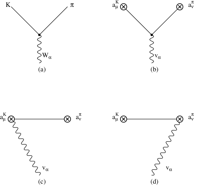
Figure 2: (a) The diagram for $K\to\pi W$ in the standard Feynman Diagram approach; (b-d) the diagrams in the external field method.

The amplitude for the process $K(p_{K})\to\pi(p_{\pi})W$ from the diagram in Fig. 2a is given by

$${}A=\frac{i}{\sqrt{2}}\left(p_{\pi}+p_{K}\right)_{\alpha}W^{\alpha}\ .$$ (3.4)

In the limit of equal quark masses this amplitude satisfies the correct behaviour only on-shell, i.e. $p_{\pi}^{2}=p_{K}^{2}=m_{\pi}^{2}$. Off-shell it does not vanish but is proportional to $p_{\pi}^{2}-p_{K}^{2}$ when $W^{\alpha}$ is replaced by $(p_{K}-p_{\pi})^{\alpha}$. In sharp contrast the amplitude calculated in the external field formalism corresponds to

$${}i^{3}\langle T\left(a_{\mu}^{K}v_{\alpha}a_{\nu}^{\pi}\right)\rangle=i\sqrt{(}2)F^{2}\left\{\frac{\left(p_{\pi}+p_{K}\right)_{\alpha}p_{\pi\nu}p_{K\mu}}{\left(p_{\pi}^{2}-m_{\pi}^{2}\right)\left(p_{K}^{2}-m_{K}^{2}\right)}-\frac{g_{\mu\alpha}p_{\pi\nu}}{p_{\pi}^{2}-m_{\pi}^{2}}-\frac{g_{\nu\alpha}p_{K\mu}}{p_{K}^{2}-m_{K}^{2}}\right\}\ .$$ (3.5)

The diagrams are depicted in Fig. 2(b-d). The circled crosses are insertions of the axial currents. This amplitude is well defined off-shell and satisfies the correct Ward-Identity. If the external legs are reduced and after going on-shell it agrees with Eq. (3.4). However, after making the replacement of $v^{\alpha}$ by $(p_{K}-p_{\pi})^{\alpha}$ we obtain the correct Ward identity for all values of masses and momenta. Similarly only the amplitudes which are defined using this method but with $\partial_{\mu}a^{\mu}$ satisfy the off-shell current algebra relations and not the on-shell amplitudes like in Eq. (3.4) that are extrapolated off-shell.

Let me close this session with a few simple remarks about low-energy theorems. There has been some confusion, see e.g. the discussions in [11]. The underlying problem is that there are different types of low-energy theorems and one should carefully distinguish between them. Three common types are

1. Low low-energy theorems: These are valid for photon radiation in the limit of vanishing photon mass as derived by Low. They relate the process with a soft-photon to the one without. This is an expansion in $E_{\gamma}$.

2. Chiral low-energy theorem: these are CHPT predictions to a given order in the chiral expansion. They relate different processes to each other in terms of the CHPT parameters to any order. These require $m_{\pi}$ and external pion momenta small. If done correctly the PCAC relations correspond exactly to these.

3. Multipole low-energy theorems: this is an expansion of the amplitudes in multipoles and then only keeping the lowest ones. In addition one often expands also in other kinematical variables and this typically requires $|E_{\pi}-m_{\pi}|<<m_{\pi}$. Their regime of validity thus requires a small kinetic energy.

In most case of interest several of these apply. E.g., in $\gamma N\to\pi N$ both 2. and 3. apply and the amplitudes of Bernard et al. [20] satisfy the multipole expansion if the expansion in $(E_{\pi}-m_{\pi})$ is done. They do also show that this expansion has a very small domain of validity.

4 Next-to-Leading Order and the Values of its Parameters

At the next-to-leading order there are 12 terms plus the Wess-Zumino term. The explicit form of the Lagrangian can be found in Refs. [2] to [9]. The Wess-Zumino term describes the anomaly and has a fixed coefficient. Of the remaining 12 terms two are not measurable. They correspond to specific choices of the external field renormalization in QCD. So we have 10 new parameters that need to be determined experimentally.

In addition there are ambiguities in the effective theory itself in identifying the quark masses. The reason is that $\chi^{\prime}=\left(\chi^{\dagger}\right)^{-1}\det\chi$ has the same transformation properties as $\chi$ under the chiral group. Replacing $\chi$ by $\chi+\beta\chi^{\prime}$ corresponds to a shift in the values of $L_{6}$, $L_{7}$ and $L_{8}$ and $m_{u}\to m_{u}+\alpha m_{d}m_{s}$. This is known as the Kaplan Manohar ambiguity[21]. This problem has two solutions:

1. $\chi^{\prime}$ transforms differently under $U(1)_{A}$ then $\chi$[22].

2. go to QCD directly. This is equivalent to calculating the relevant coefficients $L_{i}$ thus fixing the ’shift’.

The latter approach has been done in the QCD sum rule and lattice determination of quark masses:

$$2\hat{m}=(m_{u}+m_{d})(1~{}{\rm GeV}^{2})=12\pm 2.5~{}{\rm MeV}$$ (4.1)

as derived in ref. [23] and

$$m_{s}(1~{}{\rm GeV}^{3})=175\pm 25~{}{\rm MeV}$$ (4.2)

from Refs. [24]. In [23] the quark vacuum expectation value was also determined:

$$\frac{1}{2}\langle\overline{u}u+\overline{d}d\rangle=-(0.013\pm 0.003)~{}{\rm GeV}^{3}=-(235~{}{\rm MeV})^{3}\ .$$ (4.3)

This leads to a large value for $B_{0}$ and a small ($\approx$3.5%) correction to the Gell-Mann-Oakes-Renner relation. We can add in addition the relation [2]

$$\frac{m_{d}-m_{u}}{m_{d}+m_{u}}=\frac{m_{\pi}^{2}}{m_{K}^{2}}\frac{\left(m_{K^{0}}^{2}-m_{K^{+}}^{2}\right)_{QCD}}{m_{K}^{2}-m_{\pi}^{2}}\frac{m_{s}^{2}\hat{m}^{2}}{4\hat{m}^{2}}$$ (4.4)

together with determination of the electromagnetic part of the mass difference[25] to obtain

$$\frac{m_{u}}{m_{d}}=0.44\pm 0.22\ .$$ (4.5)

Notice that the numbers above lead to $m_{s}/\hat{m}=29\pm 7$, very close to the current algebra values.

Using these quark mass values the values of the $L_{i}$ can then be determined [2, 10]. These are in Table 1 where I have also listed the source of the experimental information used.

$L_{i}$	Value $\cdot 10^{3}$	Input
1	$0.4\pm 0.3$	$K_{e4}$ and $\pi\pi\to\pi\pi$
2	$1.35\pm 0.3$	$K_{e4}$ and $\pi\pi\to\pi\pi$
3	$-3.5\pm 1.1$	$K_{e4}$ and $\pi\pi\to\pi\pi$
4	$-0.3\pm 0.5$	$1/N_{c}$ arguments
5	$1.4\pm 0.5$	$F_{K}/F_{\pi}$
6	$-0.2\pm 0.3$	$1/N_{c}$ arguments
7	$-0.4\pm 0.2$	GMO, $L_{5}$, $L_{8}$
8	$0.9\pm 0.3$	$m_{K^{0}}-m_{K^{+}}$, $L_{5}$, baryon mass ratios
9	$6.9\pm 0.7$	pion electromagnetic charge radius
10	$-5.5\pm 0.7$	$\pi\to e\nu\gamma$

Table 1: The values of the $L_{i}$ coefficients and the input used to determine them, they are quoted at a scale $\mu=m_{\rho}$.

Now the first three are from $K\to\pi\pi e\nu$[26]. In amplitudes they are determined from the formfactor. As an example I quote the $s$ wave one at threshold. The lowest order calculation gives $f_{S}(0)=3.74$ and the experimental determination was $f_{S}(0)=5.59\pm 0.14$. So there is a 50% correction going to higher order. The question is can we now trust a next-to-leading order calculation. We can answer part of this since the sources of large higher order corrections are known. We can then use the strategy (see [27]) of using dispersion relations and determining the subtraction constants using CHPT to estimate the higher orders. This was done in Ref. [26] for the first three coefficients. We obtained $L_{1(2)}=0.60(1.5)\cdot 10^{-3}$ at the one-loop accuracy and $L_{1(2)}=0.37(1.35)\cdot 10^{-3}$ estimating the higher orders with dispersion relations. So the size of the higher orders seems under control for these processes.

5 Order $p^{6}$

The situation at order $p^{6}$ is somewhat less complete. There exists a classification of all terms in the Lagrangian at this order[28]. For the sector including an odd number of Levi-Civita tensors ($\varepsilon^{\mu\nu\alpha\beta}$), a lot of calculations exist and the general infinity structure is known[29]. In this case $p^{6}$ is the next-to-leading order. Some two-loop calculations also exist. In particular the $p^{6}$ correction to $\gamma\gamma\to\pi^{0}\pi^{0}$ is known[30] and several more calculations are in progress.

Figure 3: Experimental results (crosses), $p^{4}$ calculation (dashed), $p^{6}$ calculation (full) and dispersive estimates (dash-dotted), taken from Ref. [30].

In Fig. 3 I have shown the effect of the one-loop calculation for $\gamma\gamma\to\pi^{0}\pi^{0}$. This was in fact a parameter free prediction. The dispersive calculation and the $p^{6}$ calculation are in impressive agreement with each other and with the data.

In general calculations at this order are technically very demanding and still contain a reasonably large number of free parameters. It thus becomes necessary to estimate those coefficients from other sources.

6 Estimates of Parameters

The first attempts at estimating the $L_{i}$ from underlying physics arguments were done in Refs. [31, 32, 33] and in Ref. [34] for the anomalous sector. The basic idea is that formfactors are dominated by resonance exchange. E.g., the pion electromagnetic form factor is dominated by $\rho$ exchange, $F_{\pi}(q^{2})\approx 1/\left(1-q^{2}/m_{\rho}^{2}\right)$, leading to the prediction $L_{9}=F_{V}G_{V}/(2m_{\rho}^{2})$. This type of estimates was used in the calculation in Ref. [30]. In the anomalous sector there is a problem with trying to implement full meson dominance[35] but one can still estimate the order $p^{6}$ parameters.

One can also use constraints from high energy behaviour[32].

The third avenue is to calculate them from models intermediate between QCD and CHPT. A most prominent example is the calculation in the ENJL model. See Ref. [36] and references therein. This model in fact leads to most of the meson dominance relations obtained using the first method.

7 Inclusion of Nonleptonic Weak and Electromagnetic Interactions

Here we need to construct terms in the effective Lagrangian that corresponds to the nonleptonic part of the electromagnetic and weak interaction. Let me concentrate on the electromagnetic example. The underlying effective action is

$${}{\cal H}_{\rm eff}=\int d^{4}q\frac{-ie^{2}}{q^{2}}\left(g_{\mu\nu}-\frac{q_{\mu}q_{\nu}}{q^{2}}\right)J_{\rm em}^{\mu}J_{\rm em}^{\nu}\ .$$ (7.1)

This effective Hamiltonian transforms under $SU(3)_{L}\times SU(3)_{R}$ as $\left(8_{L}+8_{R}\right)^{2}$. So we now need to construct terms using the CHPT external fields and degrees of freedom, $U$, that transform in this fashion. This we do via introducing spurion fields. These fields are dummy fields that are added to the terms like Eq. (7.1) to make them singlets under the chiral group. This procedure is similar to the one used for inclusion of the quark masses. The term $\overline{q}_{i}q_{i}$ is made invariant by introducing the scalar field $s$. $-s^{ij}\overline{q}_{i}q_{j}$ has singlet properties under the chiral group. In the chiral Lagrangian we then include the field $s$ via $\frac{2B_{0}F^{2}}{4}{\rm tr}\left(sU+U^{\dagger}s\right)$. The quark masses are then included later via $s={\rm diag}\left(m_{u},m_{d},m_{s}\right)$.

The same thing can now be done for the nonleptonic Lagrangians. Eq. (7.1) contains a term $\chi^{ij}_{L}\chi^{kl}_{R}\quad\overline{q}_{iL}\gamma_{\mu}q_{jL}\quad\overline{q}_{kR}\gamma^{\mu}q_{lR}$. This is made invariant by making $\chi_{L}$ and $\chi_{R}$ transform as left and right handed octets under the chiral group. There are then two terms that can be constructed at lowest order:

$$c\;{\rm tr}\left(\chi_{R}U\chi_{L}U^{\dagger}\right)+d\;{\rm tr}\left(\chi_{L}^{2}+\chi_{R}^{2}\right)\ .$$ (7.2)

Putting in the right values for $\chi^{ij}_{L}$ and $\chi^{kl}_{R}$ this term is then responsible for the $\pi^{+}-\pi^{0}$ mass difference. At higher orders one can then similarly construct all terms.

Unfortunately this leads to very large numbers of terms at next-to-leading(NLO) order. For the nonleptonic electromagnetic case these have been classified by Urech[37]. As shown above at lowest order there are 2, one of which is a pure counterterm. At NLO there are 15. Here in fact there are large corrections expected[25].

In the weak nonleptonic sector the terms and the associated infinity structure has been classified by Kambor et al. [38]. Here there is one parameter at leading order each for octet and 27 (or $\Delta I=3/2$) transitions but at NLO there are 48 parameters in the octet case and 34 for the 27 case. Here it thus becomes very important to be able to estimate these from other sources. The main problem is that, as in Eq. (7.1) there is an integration over the momentum of an external gauge field. This problem thus involves the strong interaction at all scales. The main attempts are done using factorization, quark models [39], ENJL[40] and various sum rules[27]. See also the references in these papers.

8 Inclusion of non Goldstone Boson Fields

a) Vector Mesons: In this sector we loose pure CHPT power counting since due to the diagram of Fig. 4 whenever there is a vector meson on-shell present, it always involves large momenta for the pseudoscalars in the intermediate state.

Figure 4: A diagram creating problems for power counting in CHPT including on-shell vector mesons.

The problem is then that we need counterterms involving pions to all orders. This does not invalidate the discussion in Sect. 6, there the vector meson was at low momentum. In general the use of effective Lagrangians for meson fields can still be useful (see E.g. the talks by Ko and Pisarski in these proceedings). The choice of interpolating field for the $\rho$ is free. This leads to the different representations for the vector field:

1. The Gauged Yang-Mills version

2. Hidden Local gauge Symmetry version

3. Using the standard CCWZ mechanism (see in [7])

4. The anti-symmetric tensor field representation, used in [31]

These are all equivalent but some choices of parameters look nice in one version and ugly in another one. As an example, the vector meson decay vertex looks very different in all models. It is

$$\rho_{\mu}\left[\Phi,\partial^{\mu}\Phi\right]$$ in model 1 and 2;

$$\partial_{\mu}\rho_{\nu}\left[\partial^{\mu}\Phi,\partial^{\nu}\Phi\right]$$ in model 3 and

$$\rho_{\mu\nu}\left[\partial^{\mu}\Phi,\partial^{\nu}\Phi\right]$$ in model 4. (8.1)

So one sees that even the number of derivatives in the interaction is representation dependent. These are all on-shell equivalent. They also become off-shell equivalent if the correct pointlike pion couplings are included, see e.g. Ref. [32].

Version 3 even has no obvious vector meson dominance for the pion charge radius. Its contribution starts only at order $p^{6}$. The equivalence between the different models is obvious when we start from an underlying quark model, see e.g. [36] since then it becomes a choice for the auxiliary variable.

b) Nucleons: Here CHPT is possible for some processes. I.e. those where the conservation of baryon number allows us to systematically keep the heavy nucleon mass locked up inside the nucleon. Then the pion momenta can remain small and the problem of Fig. 4 does not occur. As an example, the process $p\overline{p}\to\pi\pi$ is definitely not treatable using CHPT but $\pi p\to\pi p$ probably is[20]. Best is to choose a formulation where the heavy mass is obviously absent from the pion momenta. this can be done using nonrelativistic field theory for the nucleons or using heavy baryon CHPT (see [5] and references therein).

Here there are a lot of problems and challenges.

1. The number of parameters is very large.

2. The mass gap between lowest states and excitations is much smaller: $\Delta=m_{\Delta}-m_{N}\approx m_{\pi}$. In fact one can also do a rigorous perturbation expansion choosing $\Delta$ as small and then doing an expansion in $\Delta,m_{\pi},\vec{p}_{N},\vec{p}_{\Delta}$ and $p_{\pi}$.

3. In the traditional view $\Delta$ is taken as large[5].

In fact case 2 seems to follow from assumptions about leading $1/N_{c}$[41] or about the spectrum[42].

The field of many nucleons is also not well developed. One qualitative conclusion is that chiral symmetry explains the observed smallness of the 3-body potential[43]

9 Conclusions

The present state of CHPT can be summarized simply. It is a mature field for processes with mesons only, it is in its adolescent stage for calculations involving one nucleon or one baryon and the many nucleon-baryon sector is in its infancy.

CHPT is a useful technique despite its large number of free parameters. It is a theory, not a model. This means that it also tells us when the corrections are very large and its predictions thus unreliable. The technique also allows us to use the full field theory machinery to its full advantage.

This talk contained some discussions about the general method and some examples of uses of CHPT. In the latter I have emphasized the work I have been involved in.

10 Acknowledgements

I would like to thank the organizers and their students for a pleasant and well organized meeting.

References

- [1] J. Gasser and H. Leutwyler, Ann. Phys. (NY) 158 (1984) 142
- [2] J. Gasser and H. Leutwyler, Nucl. Phys. B250 (1985) 465, 517
- [3] E. de Rafael, Chiral Lagrangians and Kaon CP-violation, lectures given at TASI 94, Boulder, Colorado, to be published in the proceedings, CPT-95/P.3161, hep-ph/9502254
- [4] G. Ecker, Chiral Perturbation Theory, UWThPh-1994-49, hep-ph/9501357
- [5] V. Bernard, N. Kaiser and U.-G. Meißner, Chiral Dynamics in Nucleons and Nuclei, CRN 95/3, TK 95 1, hep-ph/9501384, to be published in Int. J. Mod. Phys. E
- [6] A. Pich, Chiral Perturbation Theory, FTUV/95-4 , IFIC/95-4, hep-ph/9502366
- [7] J. Donoghue, E. Golowich and B. Holstein, Dynamics of the Standard Model (Cambridge University Press, Cambridge, 1992)
- [8] L. Maiani, G. Pancheri and N. Paver, eds., The DANE Physics Handbook, INFN-Frascati, Frascati, 1992, a new edition is scheduled to appear in spring 95
- [9] J. Bijnens, G. Ecker and J. Gasser, Chiral Perturbation Theory, in [8], hep-ph/9411232
- [10] J. Bijnens et al., Semileptonic Kaon Decays, in [8], hep-ph/9411311
- [11] A. Bernstein and B. Holstein, Proceedings of the MIT workshop on Chiral Dynamics, to be published
- [12] M. Neubert, Phys. Rep. 245 (1994) 261
- [13] S. Weinberg, Physica 96A (1979) 327
- [14] H. Leutwyler, Ann. of Phys. (NY) 235 (1994) 165
- [15] E. D’Hoker and S. Weinberg, Phys. Rev. D50 (1994) 6055
- [16] H. Leutwyler, Phys. Rev. D49 (1994) 3033
- [17] S. Weinberg, Phys. Rev. Lett. 17 (1966) 616
- [18] J. Bijnens et al., work in progress
- [19] V. Thorsson and A. Wirzba, S-Wave meson nucleon interactions and the meson mass in nuclear matter from chiral effective Lagrangians, NORDITA 95/7 N, nucl-th/9502003
- [20] N. Kaiser, these proceedings, see also [5] and references therein
- [21] D. Kaplan and A. Manohar, Phys. Rev. Lett. 56 (1986) 2004
- [22] J. Donoghue and D. Wyler, Phys. Rev. D45 (1992) 892
- [23] J. Bijnens, J. Prades and E. de Rafael, Light Quark Masses in QCD, NORDITA-94/62 N,P, hep-ph/9411285, to be published in Phys. Lett. B
-
[24]
M. Jamin and M. Münz, The strange Quark Mass from
QCD sum rules, CERN-TH.7435/94,hep-ph/9409335;
K. Chetyrkin et al., Mass singularities in light quark correlators: the strange quark case, MZ-TH/94-21, hep-ph/9409371 -
[25]
J. Donoghue, B. Holstein and
D. Wyler, Phys. Rev. D47 (1993) 2089;
J. Bijnens, Phys. Lett. B306 (1993) 343 - [26] J. Bijnens, G. Colangelo and J. Gasser, Nucl. Phys. B427 (1994) 427
- [27] J. Donoghue, these proceedings
- [28] H.W. Fearing and S. Scherer, Extension of the Chiral Perturbation Theory Meson Lagrangian to , TRI-PP-94-68, hep-ph/9408346
-
[29]
For a review see J. Bijnens, Int. J. Mod. Phys.
A8 (1993) 3045;
Ll. Amettler et al., Phys. Lett. B303 (1993) 140 - [30] S. Bellucci, J. Gasser and M. Sainio, Nucl. Phys. B423 (1994) 80
- [31] G. Ecker et al., Nucl. Phys. B321 (1989) 311
- [32] G. Ecker et al. Phys. Lett. B223 (1989) 425
- [33] J. Donoghue, C. Ramirez and G. Valencia, Phys. Rev. D39 (1989) 1947
- [34] J. Bijnens, A. Bramon and F. Cornet, Z. f. Phys. C46 (1990) 599
- [35] J. Bijnens and J. Prades, Phys. Lett. B320 (1994) 130
- [36] J. Bijnens, Ch. Bruno and E. de Rafael, Nucl. Phys. B390 (1993) 501; J. Bijnens, Chiral Lagrangians and Nambu-Jona-Lasinio like Models, NORDITA - 95/10 N,P, hep-ph/9502335
- [37] R. Urech, Nucl. Phys. B433 (1995) 234
- [38] J. Kambor, J. Missimer and D. Wyler, Nucl. Phys. B346 (1990) 17
-
[39]
A. Pich and E. de Rafael, Nucl. Phys. B358 (1991) 311;
Ch. Bruno and J. Prades, Z. f. Phys. C57 (1993) 585 - [40] J. Bijnens and J. Prades, Phys. Lett. B342 (1995) 331; The -Parameter in the Expansion, NORDITA - 95/11 N,P, hep-ph/9502363
- [41] R. Dashen, E. Jenkins and A. Manohar, Phys. Rev. D49 (1994) 4713
- [42] S. Weinberg, Strong Interactions at Low Energies, UTTG-16-94, hep-ph/9412326
- [43] S. Weinberg, Phys. Lett. B295 (1992) 114