TTP95–05

hep-ph/9502375

February 1995

QCD Corrections to Electroweak Annihilation Decays of Superheavy Quarkonia

J. H. Kühn and M. Peter

Institut für Theoretische Teilchenphysik
Universität Karlsruhe
D–76128 Karlsruhe, Germany

QCD corrections to all the allowed decays of superheavy groundstate quarkonia into electroweak gauge and Higgs bosons are presented. For quick estimates, approximations that reproduce the exact results within less than at worst two percent are also given.

I Introduction

The search for new quark flavors remains an important and interesting task. The existence of a fourth generation cannot be excluded on the basis of present measurements. The $\rho$-parameter only restricts the possible mass-splitting and the limit on the ‘number of neutrinos’ refers to light ones only. In fact, some GUTs even require quarks that do not fit into the standard model scheme.

Because charm as well as bottom have been discovered through hadronic production of their quarkonium bound states $J/\psi$ and $\Upsilon$ respectively, some authors [4, 6] examined the prospects for discovering new flavors at future hadron colliders through a similar mechanism. Given favorable circumstances, gluon fusion would be the dominant source for quarkonium production and therefore especially the pseudoscalar ground state $\eta$ could be produced with sufficient rate. Also the ${}^{3}S_{1}$ state $\psi$ might be accessible.

For the lighter member of a fourth generation doublet the single quark decay, i.e. the decay of one of the constituents in the quarkonium, is likely to be suppressed due to small intergeneration mixing angles. Thus one may in a first step ignore this channel and only consider the annihilation decays. The latter include some new and distinctive modes which may even become dominant. The most important one could be $\eta\to ZH$, which might even offer a way to discover the Higgs boson [4, 5].

Predictions for the decays $\eta,\psi\to\gamma\gamma,\gamma Z,ZZ,WW,ZH$ have been derived in Born approximation in references [2, 3, 4]. QCD corrections, however, are only partly known. The aim of this work is to fill this gap.

The paper is organized as follows: The calculational method employed can be found in [1] and will be discussed only briefly in the following section II, together with some general considerations. In section III the results of our calculations will be presented. Compact approximations will be given in section IV, a brief summary in section V.

II General considerations

Not yet discovered quarks must be heavy and a nonrelativistic treatment of their bound states is adequate. As is well known, in this case the decay width of an S-wave bound state factorizes into a nonperturbative part – the wavefunction at the origin – and a perturbative part which is proportional to the free quark scattering cross section:

$$d\Gamma(S\to p_{1}+p_{2})=\frac{1}{4m^{2}}\frac{|R_{S}(0)|^{2}}{4\pi}|{\cal M}(\vec{v}=0)|^{2}d_{Lips}$$ (1)

where $\vec{v}$ denotes the relative velocity of the $q\bar{q}$ system and $\cal M$ the free scattering amplitude. The factorization in this form applies for S-states only (for P-states see [1]) and to the order considered in this paper. Relativistic corrections first enter at ${\cal O}(\alpha_{S}^{2})$, not considered in this work.

There are several ways to calculate the rate: one is to simply compute the spin averaged cross section (with a modified statistical factor $1/4\to 1/(2S+1)$ where $S$ refers to the spin of the bound state), if only the desired spin configurations can contribute to the sum. This may require care concerning possible couplings. Consider for example the $\gamma H$-mode: among the S waves only the spin 1 state with $J^{PC}=1^{--}$ can decay that way, and the approach is straightforward. However, if we switch to the $ZH$-mode, both states with $J^{PC}=0^{-+}$ and $J^{PC}=1^{--}$ are present in the sum, albeit with unknown relative weight. In this case one may identify the parity violating part $\propto a\cdot v$ in the amplitude with the $\eta$ decay, the part $\propto(v^{2}+a^{2})$ with $\psi$. A second way is to project the appropriate amplitudes using the method derived in [1]. Both methods were used to obtain and check the results given below, with the exception of the decays into two $W$s. There only the second one was applied because the separation of the various couplings is inconvenient.

The calculation of the wavefunction $R_{S}$ requires the knowledge of the QCD potential. To get rid of the dependence on the potential model all widths are normalized to

$$\Gamma(\eta\to\gamma\gamma)=12|R_{S}(0)|^{2}\frac{\alpha^{2}Q^{4}}{M^{2}}$$ (2)

and only the ratios

$$R^{X}_{ab}\equiv\frac{\Gamma(X\to ab)}{\Gamma(\eta\to\gamma\gamma)}$$ (3)

are presented.

The zeroth order generic Feynman diagrams responsible for the annihilation decays are shown in Fig. 1. The decay through the virtual photon or $Z$ (Fig. 1(a)) contributes only to the channel $W^{+}W^{-}$, the decay through the virtual Higgs (Fig. 1(b)) is shown only for completeness. It contributes neither to $\eta$ nor to $\psi$ decays because of its quantum numbers (this only applies to a standard model Higgs, of course).

First order QCD corrections receive contributions from the diagrams shown in Fig. 2. Their sum is infrared finite. Real gluon emission is forbidden by color conservation. Comparing this result with the calculation of QED corrections, which is practically the same in this order, we could also argue that the coupling of real gluons (photons) to a color (electrically) neutral state vanishes in the static limit, thus providing an infrared finite answer.

However, as expected, all corrections exhibit the Coulomb singularity, e.g.

$$\Gamma(\eta\to\gamma\gamma)=\Gamma^{(Born)}(\eta\to\gamma\gamma)\left(1+\frac{\alpha_{s}C_{F}}{2\pi}\left(\frac{\pi^{2}}{|\vec{v}|}+\frac{\pi^{2}}{2}-10\right)\right)$$ (4)

which is universal, proportional to $1\over|\vec{v}|$ ($C_{F}=4/3$ is a color factor), and which originates from box- and from s-channel vertex correction diagrams (Figs. 2(a) and (d)). This divergence actually represents part of the Bethe-Salpeter wavefunction and must be dropped since it is already included in the factor $R_{S}(0)$. Furthermore, since we are calculating ratios of decay widths, the singularities (formally) cancel anyway. The K-factors for the ratios $R$, and their nontrivial parts $\delta k$, which are defined through

$$K^{X}_{ab}\equiv\left(R^{X}_{ab}\right)_{corrected}:\left(R^{X}_{ab}\right)_{Born}=1+\frac{\alpha_{s}C_{F}}{2\pi}\cdot\delta k^{X}_{ab}$$ (5)

will thus be free from Coulomb singularities. The corrected rate can then be obtained from

$$\Gamma^{X}_{ab}=\Big{(}R^{X}_{ab}\Big{)}_{Born}\cdot\Gamma^{Born}(\eta\to\gamma\gamma)\cdot\Big{(}1+\frac{\alpha_{S}C_{F}}{2\pi}\Big{(}\frac{\pi^{2}}{2}-10+\delta k^{X}_{ab}\Big{)}\Big{)}$$ (6)

FIG. 1.: Tree level generic Feynman diagrams

FIG. 2.: Diagrams contributing to first order QCD corrections

At this point a comment on the regularization the Coulomb singularity is appropriate. Two different procedures are possible: one may either start with nonvanishing $\beta$ and consider the limit $\beta\to 0$ in the end, which obviously requires significantly more effort during the calculation than really needed, in particular for the box diagram. Alternatively one may set $\beta=0$ from the outset and employ a nonvanishing gluon mass $\lambda$. This second procedure has several advantages: the Coulomb singularity and the infrared divergences are regularized in one step and the special kinematical situation facilitates the calculation (especially of the box diagram) significantly. To connect the two approaches the vertex correction can be investigated. This leads to the substitution rule

$\displaystyle\frac{m}{\lambda}\widehat{=}\frac{\pi}{4|\vec{v}|}.$

Before the results of the calculations can be presented, the notation must be fixed. Vector and axial vector coupling constants are abreviated with the help of

$\displaystyle v=2(I_{3L}+I_{3R})-4Q\sin^{2}\Theta_{w}\quad,\quad a=2(I_{3L}-I_{3R})\quad,\quad y=2\sin 2\Theta_{W}$

where $Q$ denotes the quark charge divided by the proton charge, $I_{3}$ (the 3-component of) the weak isospin and $\Theta_{w}$ the weak mixing angle. The results are applicable to fourth generation quarkonia as well as to more unconventional quarks (for example an isosinglet in $E_{6}$ models) as long as the couplings to the Higgs boson coincide with those of the standard model.

All masses are measured in units of the quarkonium mass $M=2m_{q}$, whence $\rho_{X}=M_{X}^{2}/M^{2}$.

III Results

A Decays into $ZZ$ or $\gamma\gamma$

Decays into two Z bosons are possible if the mass $M$ of the quarkonium is larger than twice the Z mass and proceed via diagrams 1(a,c,d). $\psi\to\gamma\gamma$ is forbidden by C conservation, whereas $\psi\to ZZ$ is allowed through the parity violating coupling. $\Gamma(\eta\to\gamma\gamma)$ can be obtained from $\Gamma(\eta\to ZZ)$ by replacing $a\to 0,~{}v\to Qy$ and taking the limit $\rho_{Z}\to 0$, which leads to the result given above (2). The lowest order predictions for the ratios

$$R^{\eta}_{ZZ} = \frac{(v^{2}+a^{2})^{2}}{(Qy)^{4}}\frac{\beta^{3}}{(1-2\rho_{Z})^{2}}$$ (7)

$$R^{\psi}_{ZZ} = \frac{2}{3}\frac{(av)^{2}}{(Qy)^{4}}\frac{\beta^{5}}{\rho_{Z}(1-2\rho_{Z})^{2}}$$ (8)

where $\beta=\sqrt{1-4M_{Z}^{2}/M^{2}}$ in this case, are well known. To include the QCD corrections, they have to be multplied by the K-factors, which contain as their nontrivial parts:

$$\delta k^{\eta}_{ZZ} = -\frac{1-\beta^{2}}{\beta^{2}}-\frac{\pi^{2}}{2}+\frac{1+3\beta^{2}-5\beta^{4}+\beta^{6}}{\beta^{4}}\ln(1+\beta^{2})-8\frac{2+5\beta^{2}-\beta^{4}}{\beta^{2}(1+\beta^{2})}B(\rho_{Z})$$ (10)

$$-2\frac{1+\beta^{2}}{\beta^{2}}C(\beta)+\frac{8a^{2}(1+\beta^{2})}{(v^{2}+a^{2})\beta^{2}}\Bigg{(}\ln(1+\beta^{2})+\frac{8}{1+\beta^{2}}B(\rho_{Z})+C(\beta)\Bigg{)}$$

$$\delta k^{\psi}_{ZZ} = 2-\frac{\pi^{2}}{2}-\frac{2-3\beta^{2}+4\beta^{4}+\beta^{6}}{\beta^{4}}\ln(1+\beta^{2})-4\frac{6+7\beta^{2}+11\beta^{4}+2\beta^{6}}{\beta^{4}(1+\beta^{2})}B(\rho_{Z})$$ (12)

$$-\frac{6+\beta^{2}-9\beta^{4}}{2\beta^{4}}(1+\beta^{2})C(\beta)$$

$$B(\rho_{Z}) = \sqrt{\rho_{Z}(1-\rho_{Z})}\arcsin\sqrt{\rho_{Z}}$$

$$C(\beta) = -\frac{1}{2\beta}\Bigg{\{}\frac{\pi^{2}}{4}+\mathop{\rm Li_{2}}\nolimits\Bigg{[}-\Bigg{(}\frac{1-\beta}{1+\beta}\Bigg{)}^{2}\Bigg{]}-\mathop{\rm Li_{2}}\nolimits\Bigg{[}\Bigg{(}\frac{1-\beta}{1+\beta}\Bigg{)}^{2}\Bigg{]}$$

$$\quad+2\Re\Bigg{[}\mathop{\rm Li_{2}}\nolimits\Bigg{(}\frac{1-\beta}{1-i\beta\sqrt{\frac{3+\beta^{2}}{1-\beta^{2}}}}\Bigg{)}-\mathop{\rm Li_{2}}\nolimits\Bigg{(}\frac{1+\beta}{1+i\beta\sqrt{\frac{3+\beta^{2}}{1-\beta^{2}}}}\Bigg{)}\Bigg{]}\Bigg{\}}$$

$\mathop{\rm Li_{2}}\nolimits(x)$ denotes the dilogarithm: $\mathop{\rm Li_{2}}\nolimits(x)=-\int_{0}^{1}dt\frac{\ln(1-xt)}{t}$.

FIG. 3.: $K_{ZZ}$ and $\delta k_{ZZ}$

The limiting case of a large quarkonium mass as well as shorter approximate formulæ are presented in section IV.

The two K-factors are shown in Fig. 3, using [6]:

$\displaystyle\alpha_{S}(M^{2})=\frac{12\pi}{21\ln(M^{2}/\Lambda^{2})}\quad\mbox{with}\quad\Lambda=58MeV$

The leading apparent singularities of $K^{\psi}_{ZZ}$ and $K^{\eta}_{ZZ}$ at threshold ($M=2M_{Z}$ or $\beta=0$) proportional to $1/\beta^{4}$ and $1/\beta^{2}$ respectively cancel. Hence $K^{\psi}_{ZZ}$ diverges $\propto 1/\beta^{2}$, $K^{\eta}_{ZZ}$ remains finite:

$$\delta k^{\eta}_{ZZ} \to \frac{29}{6}-\frac{\pi}{\sqrt{3}}-\frac{\pi^{2}}{2}+\frac{1-\sqrt{3}\pi}{3}\frac{8a^{2}}{v^{2}+a^{2}}\qquad\beta\to 0$$ (13)

$$\delta k^{\psi}_{ZZ} \to \frac{\sqrt{3}\pi}{\beta^{2}}+\frac{16}{3}-\frac{43\pi}{5\sqrt{3}}-\frac{\pi^{2}}{2}\qquad\beta\to 0$$ (14)

The D-wave phase space $\propto\beta^{5}$ for $\psi\to ZZ$ which is present in Born approximation is thus modified to a behavior $\propto\beta^{3}$ characteristic for P-wave phase space.

B Decays into $Z\gamma$

The decay to a Z boson plus a photon is possible if the quarkonium mass exceeds the Z mass. The t- and u-channel quark exchange diagrams (c) and (d) contribute. The normalized decay rates are given by

$$R^{\eta}_{Z\gamma} = 2\frac{v^{2}}{(Qy)^{2}}\beta$$ (15)

$$R^{\psi}_{Z\gamma} = \frac{2}{3}\frac{a^{2}}{(Qy)^{2}}\frac{\beta(2-\beta)}{(1-\beta)^{2}}$$ (16)

(with $\beta=1-M_{Z}^{2}/M^{2}$) and the K-factors by

$$\delta k^{\eta}_{Z\gamma} = 2\frac{1-\beta}{1-2\beta}+\frac{7\pi^{2}}{6}\frac{1-\beta}{\beta}+\frac{4\beta-3\beta^{2}-1}{(1-2\beta)^{2}}\ln(2\beta)$$ (18)

$$-\frac{12}{\beta}B(\rho_{Z})-2\frac{3-2\beta}{\beta}\arcsin^{2}\sqrt{\rho_{Z}}+2\frac{1-\beta}{\beta}\mathop{\rm Li_{2}}\nolimits(1-2\beta)$$

$$\delta k^{\psi}_{Z\gamma} = -\frac{2\beta}{1-2\beta}+\frac{\pi^{2}}{6}\frac{16-24\beta-5\beta^{2}+7\beta^{3}}{\beta^{2}(2-\beta)}-2\frac{8-39\beta+63\beta^{2}-32\beta^{3}+2\beta^{4}}{\beta(2-\beta)(1-2\beta)^{2}}\ln(2\beta)$$ (21)

$$-4\frac{8-5\beta-\beta^{2}}{\beta^{2}(2-\beta)}B(\rho_{Z})-2\frac{8-13\beta+\beta^{2}+2\beta^{3}}{\beta^{2}(2-\beta)}\arcsin^{2}\sqrt{\rho_{Z}}$$

$$+\frac{8-15\beta+2\beta^{2}+2\beta^{3}}{\beta^{2}(2-\beta)}\mathop{\rm Li_{2}}\nolimits(1-2\beta)$$

with $B(\rho_{Z})=\sqrt{\rho_{Z}(1-\rho_{Z})}\arcsin\sqrt{\rho_{Z}}$ as before.

These two functions are shown in Fig. 4.

FIG. 4.: $K_{Z\gamma}$ and $\delta k_{Z\gamma}$

Close to threshold $\beta$ approaches zero and $\delta k^{\psi}$ diverges, in contrast to $\delta k^{\eta}$. Specifically:

$$\delta k^{\psi}_{Z\gamma}\to -\Bigg{(}\frac{8\pi}{3}\Big{(}\frac{1}{\beta}\Big{)}^{1/2}+\frac{\pi^{2}}{2}-6\Bigg{)} ,~{}\beta\to 0$$ (22)

$$\delta k^{\eta}_{Z\gamma}\to -\Bigg{(}\frac{\pi^{2}}{2}-4\Bigg{)} ,~{}\beta\to 0.$$ (23)

This behavior results from the combination of the singularities of the gluon and the quark propagator. In fact, the virtual quark is close to its mass shell in this limit. Very close to threshold intermediate bound states should be taken into account since an alternative way to describe the decay is through the chain $1^{--}\to\gamma 1^{++}(\to Z)$ with mixing between $1^{++}$ and the $Z$. A similar problem also appears in $\psi\to\gamma H$ [8]. For $\beta=1/2$ the correction is regular.

C The decays into $ZH$ and $\gamma H$

As stated in the introduction the decay $\eta\to ZH$ could signal the presence of the Higgs boson and the new quark simultaneously. In Born approximation one obtains for the ratios $R$:

$$R_{ZH}^{\eta} = \frac{a^{2}}{(Qy)^{4}}\frac{\beta^{3}}{\rho_{Z}^{2}}$$ (24)

$$R_{ZH}^{\psi} = \frac{2v^{2}}{3(Qy)^{4}}\frac{\beta}{\rho_{Z}(1-\rho_{Z}-\rho_{H})^{2}}$$ (26)

$$\times\left[\left(1-\rho_{Z}-\rho_{H}\frac{1-3\rho_{Z}}{1-\rho_{Z}}\right)^{2}+\frac{\rho_{Z}}{2}\left(1-\rho_{Z}+\rho_{H}\frac{2-\rho_{H}}{1-\rho_{Z}}\right)^{2}\right]$$

with $\beta=\sqrt{1+\rho_{Z}^{2}+\rho_{H}^{2}-2\rho_{Z}-2\rho_{H}-2\rho_{Z}\rho_{H}}$. In principle, all three diagrams 1(a,c,d) could contribute to both decays. However, the contribution from (c) and (d) vanishes for $\eta\to ZH$ (this is no longer true for the QCD corrections), whereas $R^{\psi}_{ZH}$ is the sum of three terms:

$$R_{ZH,t}^{\psi} = \frac{v^{2}}{(Qy)^{4}}\frac{2\beta}{3\rho_{Z}}\frac{\beta^{2}+6\rho_{Z}}{(1-\rho_{Z}-\rho_{H})^{2}}~{}\mbox{ t-channel, (c)+(d)}$$ (27)

$$R_{ZH,s}^{\psi} = \frac{v^{2}}{(Qy)^{4}}\frac{\beta}{3}\frac{\beta^{2}+12\rho_{Z}}{(1-\rho_{Z})^{2}}~{}\mbox{ s-channel, (a)}$$ (28)

$$R_{ZH,st}^{\psi} = -\frac{v^{2}}{(Qy)^{4}}\frac{8\beta}{3}\frac{1+\rho_{Z}-\rho_{H}}{1-\rho_{Z}+\rho_{H}}~{}\mbox{ interference term}$$ (29)

For large quarkonium masses, $R^{\eta}_{ZH}$ rises proportional to $1/\rho_{Z}^{2}$, in contrast to all other modes listed up to now, which increase proportional to $1/\rho_{Z}$ or approach a constant value. The different behavior can be understood from the Goldstone boson equivalence theorem [9] which identifies the amplitudes for scattering of longitudinal gauge bosons ($Z$ or $W$) at high energies with those for the appropriate Goldstone bosons. The latter must be taken as pseudoscalar particles. The decay $\eta\to G_{Z}H$ ($G_{Z}$ denotes the Goldstone boson belonging to $Z$) is allowed, i.e. the $Z$ emitted can be longitudinal, with its coupling proportional to $M/M_{Z}$. This explains one factor $1/\rho_{Z}=M^{2}/M_{Z}^{2}$. The second one originates from the coupling of the Higgs to fermions. In contrast the decay $\psi\to G_{Z}H$ is forbidden by CP conservation, and only the transverse part of $Z$ with a coupling proportional to $g_{weak}$ remains. This leads to a rate $\propto 1/\rho_{Z}$.

The behavior of the other rates can be obtained through similar arguments: $\eta\to G_{Z}G_{Z},G_{Z}Z$ or $G_{Z}\gamma$ are forbidden, hence $R^{\eta}_{ZZ}$ and $R^{\eta}_{Z\gamma}$ approach constant values. The decays $\psi\to G_{Z}Z$ (but not $G_{Z}G_{Z}$) and $G_{Z}\gamma$ are allowed, these ratios increase $\propto 1/\rho_{Z}$.

The full expressions for the K-factors for $R_{ZH}$ can be found in the appendix. The numerical results are shown in Fig. 5. The corrections are large, at least about 15% for $R^{\eta}_{ZH}$ and 30% for $R^{\psi}_{ZH}$, but of course they do not drastically change the conclusions that can be drawn from the Born results, at least if we are not too close to threshold.

FIG. 5.: $K_{ZH}$ and $\delta k_{ZH}$ for Higgs masses $M_{H}=70,100,150,200GeV$ (solid, dashed, dotted, dash-dotted).

In the limit $\rho_{Z}\to 0$, keeping $\rho_{H}=M_{H}^{2}/M^{2}$ fixed and also keeping a factor $1/\rho_{Z}=(yg_{H}/e)^{2}$ in the numerator, the well-known result for the decay $\psi\to\gamma H$ is recovered [7]:

$$R^{\psi}_{\gamma H} = \frac{1}{(Qy)^{2}}\frac{2}{3\rho_{Z}}\Big{(}1-\rho_{H}\Big{)}$$ (30)

$$\delta k^{\psi}_{\gamma H} = 2\frac{1-3\beta}{1-2\beta}-\frac{\pi^{2}}{2}-8\frac{2-\beta^{2}}{\beta^{2}(1-\beta)}B(\rho_{H})-2\frac{4-13\beta+7\beta^{2}+8\beta^{3}}{\beta(1-2\beta)^{2}}\ln(2\beta)$$ (32)

$$+\frac{1}{\beta}\Big{(}\frac{\pi^{2}}{6}-\mathop{\rm Li_{2}}\nolimits(1-2\beta)\Big{)}+4\frac{1-\beta^{2}}{\beta^{2}}\Big{(}\frac{\pi^{2}}{3}+\mathop{\rm Li_{2}}\nolimits(1-2\beta)-2\arcsin^{2}\sqrt{\rho_{H}}\Big{)}$$

where $\beta=(1-M_{H}^{2}/M^{2})$ and $B(\rho)=\sqrt{\rho(1-\rho)}\arcsin\sqrt{\rho}$. In the same limit one obtains

$$\delta k^{\eta}_{ZH} \to 2\frac{1-4\beta}{1-2\beta}-\frac{\pi^{2}}{2}-\frac{8(2-\beta)}{(1-\beta)\beta^{2}}B(\rho_{H})-4\Big{(}\frac{2}{\beta}+\frac{1-\beta}{(1-2\beta)^{2}}\Big{)}\ln(2\beta)$$ (34)

$$+2\frac{2-\beta}{\beta^{2}}\Big{(}\frac{\pi^{2}}{3}+\mathop{\rm Li_{2}}\nolimits(1-2\beta)-2\arcsin^{2}\sqrt{\rho_{H}}\Big{)}$$

The limiting behavior of $\delta k^{\psi}_{\gamma H}$ is well known:

$$\delta k^{\psi}_{\gamma H} = -4-12\ln 2-\frac{\pi^{2}}{4}\qquad(\beta\to 1)$$ (35)

$$\delta k^{\psi}_{\gamma H} = -\frac{8\pi}{3}\frac{1}{\sqrt{\beta}}+8-\frac{\pi^{2}}{2}\qquad(\beta\to 0)$$ (36)

For $\delta k^{\eta}_{ZH}$, one obtains in the corresponding limit

$$\delta k^{\eta}_{ZH} = -2-8\ln 2\qquad(\beta\to 1)$$ (37)

$$\delta k^{\eta}_{ZH} = -\frac{8\pi}{3}\frac{1}{\sqrt{\beta}}+6-\frac{\pi^{2}}{2}\qquad(\beta\to 0)$$ (38)

D The decays into $W^{+}W^{-}$

Although the decays into $W^{+}W^{-}$ seem very similar to the decays into two $Z$, important differences arise: two distinctively different isospin assignments must be considered: case 1 for an isosinglet quark and case 2 for a standard model quark with $|I_{3}|=1/2$ (isodoublet). In case 2 the propagation of the isospin partner of the quark forming the bound state enters the diagram. Its mass is generically denoted by $m_{T}$. For an isosinglet quark (case 1), only diagram (a) is possible, and we obtain

$$R^{\eta}_{WW} = 0$$ (39)

$$R^{\psi}_{WW} = \frac{1}{Q^{2}}\frac{\beta^{3}}{48(1-\rho_{Z})^{2}}(1+20\rho_{W}+12\rho_{W}^{2})\left(\frac{M_{Z}}{M_{W}}\right)^{4}$$ (40)

In case 2, diagrams (a) and (c) contribute, and we find

$$R^{\eta}_{WW} = \frac{1}{(Q\sin\Theta)^{4}}\frac{\beta^{3}}{8(1+4\rho_{T}-4\rho_{W})^{2}}$$ (41)

$$R^{\psi}_{WW} = \frac{1}{(Q\sin\Theta)^{4}}\frac{\beta^{3}}{768\rho_{W}^{2}}\Bigg{[}(2I_{3})^{2}\frac{(1+20\rho_{W}+12\rho_{W}^{2})(1-4c\rho_{Z})^{2}}{(1-\rho_{Z})^{2}}$$ (43)

$$-16I_{3}\rho_{W}\frac{(1-4c\rho_{Z})(5+6\rho_{W})}{(1+4\rho_{T}-4\rho_{W})(1-\rho_{Z})}+16\rho_{W}^{2}\frac{2-\rho_{W}}{(1+4\rho_{T}-4\rho_{W})^{2}}\Bigg{]}$$

where

$\displaystyle\beta=\sqrt{1-4\rho_{W}}~{},~{}\rho_{T}=\frac{m_{T}^{2}}{M^{2}}~{},~{}c=2I_{3}\sin^{2}\Theta_{W}$

The dependence on the sign of $I_{3}$ which is in particular relevant for the interference term is displayed explicitly, so our result applies to up- as well as to down-type quarks. In the limit of a large quark mass, $R^{\psi}_{WW}$ rises $\propto 1/\rho_{W}^{2}$, whereas $R^{\eta}_{WW}$ approaches a constant. This again is a consequence of the equivalence theorem, which tells us that in the $\psi$ decay both $W$ can be longitudinal. In contrast both $\eta\to G_{W}G_{W}$ and $\eta\to G_{W}W$ are forbidden. Obviously the $WW$ mode would dominate $\psi$ decays.

For case 1 (isosinglet) the K-factor is simply constant:

$$\delta k^{\psi}_{WW}=2-\frac{\pi^{2}}{2}$$ (44)

The K-factors for case 2 (standard model) are again quite lengthy and are listed in the appendix. Formally $\delta k^{\eta}_{WW}=\delta k^{\eta}_{ZZ}$ if we set $m_{T}=m,~{}v=a$. Fig. 6 shows the two functions for three different values of $m_{T}$.

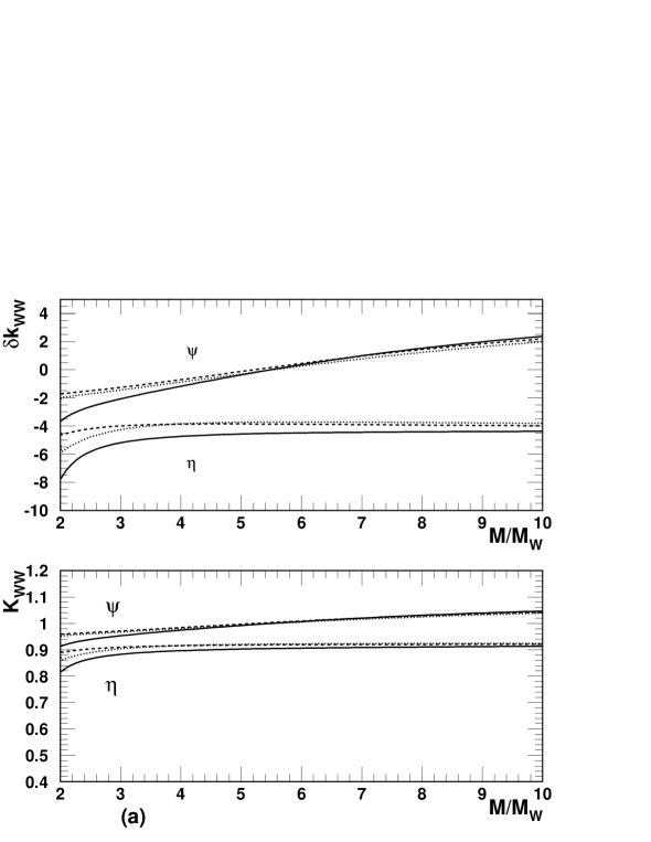
FIG. 6.: $\delta K_{WW}$ and $K_{WW}$ for down-type quarks and $m_{T}-m=0,50,80$GeV (solid, dashed, dotted).

IV Large Quarkonium mass and approximate formulÆ

The K-factors approach quickly their asymptotic behavior for $\beta$ towards zero or 1. Since additional quarks are presumably rather heavy, it often will be sufficient to take the limiting values $\rho_{X}\to 0$. They are given in table I. In the case of $WW$ a possible mass splitting between the constituent quark and its isospin partner is neglected.

Up to obvious coupling constants, the ratio between $R^{\psi}_{ZZ}$ and $R^{\psi}_{Z\gamma}$ approaches 1/2 in this limit, a consequence of the statistical factor for identical particles in the $ZZ$ case. The K-factors therefore approach the same value. Also $K^{\psi}_{ZH}$ and $K^{\psi}_{\gamma H}$ become equal, and the asymptotic value of $R^{\eta}_{ZZ}$ remains unaffected by the QCD corrections. The difference between $K^{\eta}_{ZZ}$ and $K^{\eta}_{WW}$ only arises from their different couplings to left- and right-handed quarks and the appearance of $m_{T}$ in the $WW$ case. It should be mentioned that $K^{\psi}_{WW}$ – for a down-type quark – approaches its asymptotic value very slowly, so in this case the full result given in the appendix should be used.

The following approximations are valid for the full kinematical range:

$$\delta k^{\eta}_{ZZ} \approx -5.84-4.36\rho_{Z}-47.73\rho_{Z}^{2}$$ (45)

$$\delta k^{\psi}_{ZZ} \approx \frac{\sqrt{3}\pi}{1-4\rho_{Z}}-13.66+3.09\rho_{Z}-35.41\rho_{Z}^{2}$$ (46)

$$\delta k^{\eta}_{Z\gamma} \approx -0.642\rho_{Z}-0.473\rho_{Z}^{2}$$ (47)

$$\delta k^{\psi}_{Z\gamma} \approx -\frac{8\pi}{3}\frac{1}{\sqrt{1-\rho_{Z}}}+0.1$$ (48)

They reproduce the exact result within an error of less than 1% even close to threshold.

TABLE I.: Asymptotic values of the $\delta k$-factors for $\rho_{X}\to 0$. Note that in order to obtain the full corrections, these numbers have to be multiplied by $\alpha_{S}(M)\cdot C_{F}/2\pi$.

K-factor	$\rho_{X}\to 0$	$numericalvalue$
$\delta k^{\eta}_{ZZ}$	$-\frac{2a^{2}}{v^{2}+a^{2}}(\pi^{2}-8\ln 2)$	$-5.84\leavevmode\leavevmode\hbox{${}^{\rm a}$}$
$\delta k^{\eta}_{Z\gamma}$	0	$0.0$
$\delta k^{\eta}_{ZH}$	$-2-8\ln 2$	$-7.55$
$\delta k^{\eta}_{WW}$	$-\pi^{2}+8\ln 2$	$-4.32$
$\delta k^{\psi}_{ZZ}$	$-\frac{3\pi^{2}}{4}+2-4\ln 2$	$-8.17$
$\delta k^{\psi}_{Z\gamma}$	$-\frac{3\pi^{2}}{4}+2-4\ln 2$	$-8.17$
$\delta k^{\psi}_{ZH}$	$-\frac{\pi^{2}}{4}-4-12\ln 2$	$-14.79$
$\delta k^{\psi}_{\gamma H}$	$-\frac{\pi^{2}}{4}-4-12\ln 2$	$-14.79$
$\delta k^{\psi}_{WW}$	$2(1+2I_{3})-\frac{\pi^{2}}{2}(1+4I_{3})$	$4.93\leavevmode\leavevmode\hbox{${}^{\rm a}$}^{,}\leavevmode\leavevmode\hbox{${}^{\rm b}$}$
		$-10.80\leavevmode\leavevmode\hbox{${}^{\rm c}$}^{,}\leavevmode\leavevmode\hbox{${}^{\rm b}$}$

V Summary

The complete evaluation of the QCD corrections to annihilation decays of superheavy S-state quarkonia into elektroweak (gauge) bosons has been presented. Nearly all the corrections are negative, with $\psi\to WW$ (d-type quark) being the only exception. Some of them are sizeable even in the high mass regime, where all mass scales can be neglected and the K-factors become simple constants. In particular the corrections to $\psi\to ZH$ and $\gamma H$ are of the order of 30% in this limit, whereas the others are all below 18%. The dominance of the mode $\eta\to ZH$ among the $\eta$-decays for a certain range of Higgs and quarkonium masses is not changed by strong radiative corrections.

1 Generalties

Before discussing the full analytic results for $K_{ZH}$ and $K_{WW}$, the following functions have to be introduced:

$$Q_{01} = \Big{(}\frac{m^{2}-m_{T}^{2}}{M_{H}^{2}}-1\Big{)}\ln\frac{m_{T}}{m}-2\sqrt{\Big{(}\frac{m+m_{T}}{M_{H}}\Big{)}^{2}-1}\sqrt{1-\Big{(}\frac{m-m_{T}}{M_{H}}\Big{)}^{2}}$$

$$\times\arctan\sqrt{\frac{1-\Big{(}\frac{m-m_{T}}{M_{H}}\Big{)}^{2}}{\Big{(}\frac{m+m_{T}}{M_{H}}\Big{)}^{2}-1}}$$

$$Q_{02} = Q_{01}\Big{(}M_{H}\to M_{Z}\Big{)}$$

$$Q_{12} = \frac{m_{T}^{2}-q^{2}}{q^{2}}\ln\frac{m_{T}^{2}-q^{2}}{m_{T}^{2}}-\ln\frac{m_{T}^{2}}{m^{2}}$$

$$Q_{1} = m^{2}C_{0}\big{(}m^{2},M_{Z}^{2},q^{2};0,m,m_{T}\big{)}\qquad,\qquad Q_{2}=m^{2}C_{0}\big{(}m^{2},M_{H}^{2},q^{2};0,m,m_{T}\big{)}$$

$$Q_{0} = m^{4}D_{0}\big{(}m^{2},4m^{2},m^{2},M_{H}^{2},q^{2},M_{Z}^{2};\lambda,m,m,m_{T})+\frac{m^{2}}{2(m_{T}^{2}-q^{2})}\Big{(}\ln\frac{\lambda^{2}}{m^{2}}+\frac{\pi^{2}}{2|\vec{v}|}-2\Big{)}$$

$\lambda$ is the gluon mass to regulate the infrared and Coulomb divergences as mentioned in section II, $\vec{v}$ denotes the quark velocity and the scalar three and four point one loop integrals $C_{0}$ and $D_{0}$ are defined by [10]

$$D_{0}(p_{1}^{2},(p_{1}-p_{2})^{2},p_{2}^{2},(p_{2}-p_{3})^{2},p_{3}^{2},(p_{3}-p_{1})^{2};m_{0},m_{1},m_{2},m_{3})$$

$$=\int\!\frac{d^{4}l}{i\pi^{2}}\frac{1}{[l^{2}-m_{0}^{2}][(l+p_{1})^{2}-m_{1}^{2}][(l+p_{2})^{2}-m_{2}^{2}][(l+p_{3})^{2}-m_{3}^{2}]}$$

$$C_{0}(p_{1}^{2},(p_{1}-p_{2})^{2},p_{2}^{2};m_{0},m_{1},m_{2}) = \int\!\frac{d^{4}l}{i\pi^{2}}\frac{1}{[l^{2}-m_{0}^{2}][(l+p_{1})^{2}-m_{1}^{2}][(l+p_{2})^{2}-m_{2}^{2}]}$$

In the case of $K_{ZH},~{}m_{T}=m$, which makes the expressions more compact, and for $K_{WW}$ both $M_{H}$ and $M_{Z}$ must be replaced by $M_{W}$.

When taking the limit $\lambda\to 0$ the four point function $D_{0}$ develops an infrared and a Coulomb singularity which are exactly of the displayed separately in the definition of $Q_{0}$, so the latter is finite. When calculating $Q_{0}$, it is not necessary to work out the full expression for $D_{0}$, because use can be made of the special kinematical situation which results in relations between the propagators appearing in the denominator:

$$2\lambda^{2} = [(l+p_{q})^{2}-m^{2}]+[(l-p_{q})^{2}-m^{2}]-2[l^{2}-\lambda^{2}]$$

$$2l^{2} = [(l+p_{q})^{2}-m^{2}]+[(l-p_{q})^{2}-m^{2}]$$

where $p_{q}$ is the momentum carried by the incoming quark and thus, in our approximation, $-p_{q}$ the momentum of the antiquark. These identities can be used to rewrite $D_{0}$:

$$D_{0} = \frac{1}{2\lambda^{2}}\Big{(}C_{0}(m^{2},M_{H}^{2},(p_{q}-p_{Z})^{2};\lambda,m,m_{T})-C_{0}(m^{2},M_{H}^{2},(p_{q}-p_{Z})^{2};0,m,m_{T})$$

$$+C_{0}(m^{2},M_{Z}^{2},(p_{q}-p_{Z})^{2};\lambda,m,m_{T})-C_{0}(m^{2},M_{H}^{2},(p_{q}-p_{Z})^{2};0,m,m_{T})\Big{)}$$

and the calculation is reduced to the problem of expanding three point functions, with the result:

$$Q_{0}(ZH) = \frac{1}{2z}\Big{[}d(\rho_{Z})+d(\rho_{H})\Big{]}\qquad\mbox{with}$$ (49)

$$d(\rho_{X}) = \Big{[}\frac{4\rho_{X}+z-2\beta}{z-2\beta}-\frac{z}{2-z-2\rho_{X}}\Big{]}\ln\frac{2\beta}{z}-\frac{8}{z}B(\rho_{X})+\frac{2(1-z)}{z}\Bigg{[}\frac{1}{4\rho_{X}+z-2+2\beta}$$ (53)

$$\Big{[}2\frac{4\rho_{X}-1+2\beta/z}{4\rho_{X}+z-2-2\beta+4\beta/z}\ln\frac{4\beta(1-1/z)}{z+2\beta+4\rho_{X}-2}-\ln\frac{4\beta(1-1/z)}{z(z+2\beta+4\rho_{X}-2)}\Big{]}$$

$$+\frac{1}{z-2\beta+4\rho_{X}-2}\Big{[}\frac{2(1-2\beta/z)}{z-2\beta+4\rho_{X}-2+4\beta/z}\ln\frac{4\beta/z}{2\beta+2-4\rho_{X}-z}$$

$$-\frac{z+2-4\rho_{X}-2\beta}{z-2+4\rho_{X}+2\beta}\ln\frac{4\beta}{2\beta+2-4\rho_{X}-z}\Big{]}\Bigg{]}\qquad z=2(1-\rho_{Z}-\rho_{H})$$

$$Q_{0}(WW) = -\frac{1}{z}\ln\frac{z}{t}-\frac{\sqrt{4t^{2}-z^{2}}}{z^{2}}\Bigg{[}\arctan\frac{(2-z)(2t^{2}-z)+\beta(4t^{2}-z^{2})}{\sqrt{4t^{2}-z^{2}}(2t^{2}-z-\beta(2-z))}$$ (55)

$$+\arctan\frac{(2t^{2}-z)^{2}-\beta(4t^{2}-z^{2})}{\sqrt{4t^{2}-z^{2}}(2t^{2}-z)(1+\beta)}\Bigg{]}\qquad z=t^{2}+\beta^{2},~{}t\leq 1+\frac{M_{W}}{m}$$

To demonstrate the finiteness of $Q_{0}$, a third relation can be used, which allows to explicitely split off the divergent part of $D_{0}(\lambda\to 0)$:

$\displaystyle l^{2}+2l(p_{q}-p_{Z})-[(l+p_{q}-p_{Z})^{2}-m_{T}^{2}]=m_{T}^{2}-q^{2}$

resulting in

$$D_{0}(\lambda\to 0) = -\frac{1}{m_{T}^{2}-q^{2}}C_{0}(m^{2},4m^{2},m^{2};\lambda\to 0,m,m)$$

$$+\frac{1}{m_{T}^{2}-q^{2}}\int\!\frac{d^{4}l}{i\pi^{2}}\frac{l^{2}+2l(p_{q}-p_{Z})}{l^{2}[(l+p_{q})^{2}-m^{2}][(l-p_{q})^{2}-m^{2}][(l+p_{q}-p_{X})^{2}-m_{T}^{2}]}$$

$$= \frac{1}{2m^{2}(m_{T}^{2}-q^{2})}\Big{(}\ln\frac{\lambda^{2}}{m^{2}}+\frac{\pi^{2}}{2|\vec{v}|}-2\Big{)}+\mbox{finite integral}$$

This equation, however, is not of much practical use because the calculation of the remaining finite integral by standard methods would re-introduce infrared divergencies when expanding it into two- and three-point functions.

2 K-factors for the $ZH$ mode

With these ingredients, the missing K-factors can be calculated. First the results for $K_{ZH}$:

$$\delta k^{\eta}_{ZH} = 2\frac{3-4\rho_{Z}-4\rho_{H}}{1-2\rho_{Z}-2\rho_{H}}-\frac{\pi^{2}}{2}+\left(\frac{\rho_{Z}-\rho_{H}}{\beta^{2}}+\frac{1}{1-2\rho_{Z}-2\rho_{H}}\right)2Q_{12}+4\frac{1-\rho_{Z}}{\beta^{2}}Q_{01}$$ (57)

$$+4\frac{\rho_{Z}}{\beta^{2}}Q_{02}-4\frac{1-(\rho_{H}-\rho_{Z})^{2}}{\beta^{2}}Q_{1}-8\frac{\rho_{Z}(1-\rho_{Z}+\rho_{H})}{\beta^{2}}Q_{2}+8\frac{(1-\rho_{Z}-\rho_{H})^{2}}{\beta^{2}}Q_{0}$$

The only form allowed for the amplitude for $\eta\to ZH$ is proportional to $\epsilon_{Z}\cdot P_{q\bar{q}}$. Hence the radiative corrections can trivially be written as a multiple of the Born result and the K-factor assumes a fairly simple form. However, the same consideration does not apply to $\psi\to ZH$ where two quite different and more complicated structures are present for the amplitudes on the tree level. Therefore the corrections cannot be written as a single ‘compact’ K-factor. However, the explicit calculation shows that every amplitude corresponding to a given graph of Fig. 2 can be split into two parts that are each proportional to one of the Born amplitudes. Hence, after multiplication with the latter and after spin summation, the three expressions (28) are recovered and ‘partial K-factors’ can be read off (with $z=2(1-\rho_{Z}-\rho_{H})$):

$$\delta k_{s} = \frac{1+\rho_{Z}-2z\rho_{Z}}{\rho_{Z}(1-z)}-\frac{\pi^{2}}{2}-\frac{(1-\rho_{Z})(2-3z)}{\rho_{Z}z(1-z)}Q_{12}+2F_{1}(\rho_{Z},\rho_{H})$$ (58)

$$\delta k_{st} = \frac{3(1-z)+\frac{1}{\rho_{Z}}}{2(1-z)}\!-\!\frac{\pi^{2}}{2}\!-\!\frac{\frac{2-3z}{\rho_{Z}}+(2-z-z^{2})}{2z(1-z)}Q_{12}\!+\!F_{1}(\rho_{Z},\rho_{H})\!+\!F_{2}(\rho_{Z},\rho_{H})\!+\!\frac{\rho_{Z}F_{3}(\rho_{Z},\rho_{H})}{12}$$ (61)

$$+\frac{z}{6\rho_{Z}(1+\rho_{Z}-\rho_{H})}\Big{[}\frac{3\rho_{Z}+\rho_{H}}{2}Q_{12}+(\frac{z}{4}-1)Q_{01}-\rho_{Z}Q_{02}+8\rho_{Z}(z+3\rho_{Z})Q_{0}$$

$$-\frac{4(3\rho_{Z}-1+\rho_{H})+z(1+\rho_{Z}-\rho_{H})}{4}Q_{1}+\frac{8\rho_{Z}+z(1+\rho_{Z}-\rho_{H})-2\beta^{2}}{4}Q_{2}\Big{]}$$

$$\delta k_{t} = \frac{2-z}{1-z}-\frac{\pi^{2}}{2}-\frac{4-4z-z^{2}}{z(1-z)}Q_{12}+2F_{2}(\rho_{Z},\rho_{H})+\frac{\rho_{Z}^{2}}{\beta^{2}+6\rho_{Z}}F_{3}(\rho_{Z},\rho_{H})$$ (63)

$$+\frac{z}{\beta^{2}+6\rho_{Z}}\Big{[}Q_{12}-Q_{01}+2\rho_{Z}Q_{2}+(\frac{z}{4}-1)Q_{1}+2(2\beta^{2}+12\rho_{Z}+z)Q_{0}\Big{]}$$

where

$$F_{1}(\rho_{Z},\rho_{H}) = -\frac{1-\rho_{Z}}{\rho_{Z}\beta^{2}}\Big{(}(1+\rho_{H}-\rho_{Z})Q_{01}-2\rho_{Z}Q_{02}+\frac{5\rho_{Z}-1-\rho_{H}}{2}Q_{12}$$

$$+[(\rho_{H}-\rho_{Z})^{2}-1]Q_{1}+2\rho_{Z}(1+\rho_{H}-\rho_{Z})Q_{2}\Big{)}$$

$$F_{2}(\rho_{Z},\rho_{H}) = 1-\frac{4\rho_{H}}{\beta^{2}}Q_{01}+\frac{3\rho_{Z}(1+\rho_{H}-\rho_{Z})}{\beta^{2}}Q_{02}+4\Big{[}1-\rho_{H}+\frac{\rho_{H}(1-\rho_{H}+\rho_{Z})}{\beta^{2}}\Big{]}Q_{1}$$

$$+\frac{\beta^{2}+4\rho_{Z}^{2}-4\rho_{Z}+\frac{z}{8}(4\rho_{Z}+2-z)+2\rho_{H}}{\beta^{2}}Q_{12}-\Big{[}1+4\rho_{Z}+\frac{12\rho_{Z}\rho_{H}}{\beta^{2}}\Big{]}Q_{2}$$

$$F_{3}(\rho_{Z},\rho_{H}) = \frac{z(z/4-\rho_{Z})}{\rho_{Z}^{2}(1-z)}+\frac{1}{\beta^{2}}\Big{[}[12(\rho_{Z}-1-\rho_{H})-4\frac{\beta^{2}}{\rho_{Z}}]Q_{02}+72\frac{1-\rho_{Z}}{1-z}Q_{12}$$

$$+\frac{\beta^{2}(64\rho_{Z}-20z\rho_{Z}+z^{2})+z\rho_{Z}(96\rho_{Z}^{2}-216\rho_{Z}-12+24z\rho_{Z})}{4\rho_{Z}^{2}(1-z)}Q_{12}$$

$$+2[\frac{\beta^{2}}{\rho_{Z}}(6-z)-12z+24(1-\rho_{Z})]Q_{2}\Big{]}$$

The corrected ratio is then given by

$\displaystyle R^{\psi}_{ZH}=\Big{(}R^{\psi}_{ZH}\Big{)}_{Born}+\frac{\alpha_{S}C_{F}}{2\pi}\Big{(}\delta k_{s}R^{\psi}_{ZH,s}+\delta k_{st}R^{\psi}_{ZH,st}+\delta k_{t}R^{\psi}_{ZH,t}\Big{)}$

It should be stressed, however, that the notation does not imply that for example $\delta k_{s}$ is the correction induced by the s-channel diagrams fig. 2(a,b) only. In fact, it contains part of the t-channel contribution and must be considered in the limit $M_{Z}\to 0$ to obtain the correct result for $K^{\psi}_{\gamma H}$, although on the Born level only the t-channel diagrams are possible in this limit.

3 K-factors for the $WW$ mode

The last missing K-factors are those for the decay modes $\psi\to WW$ and $\eta\to WW$. They read

$$\delta k^{\eta}_{WW} = \frac{\beta^{2}-t^{2}}{\beta^{2}}-\frac{\pi^{2}}{2}-\frac{\beta^{4}(1-\beta^{2}-2t^{2})-4\beta^{2}t^{2}-\beta^{2}t^{4}-t^{4}}{\beta^{4}}\ln\frac{t^{2}+\beta^{2}}{t^{2}}+\beta^{2}\ln(t^{2})$$ (65)

$$-(2-t^{2}-\beta^{2})Q_{02}+2\frac{t^{2}+\beta^{2}}{\beta^{2}}Q_{2}+2\frac{\beta^{4}-t^{4}}{\beta^{2}}Q_{0}$$

For $R^{\psi}_{WW}$ there are again three partial K-factors:

$$\delta k_{s} = 2-\frac{\pi^{2}}{2}$$ (66)

$$\delta k_{t} = -\frac{(\beta^{2}+t^{2})(7+t^{2}-2\beta^{2})}{\beta^{2}(7+\beta^{2})}-\frac{\pi^{2}}{2}-\frac{t^{2}(35\beta^{2}+4\beta^{4}+7t^{2}+\beta^{2}t^{2}+t^{4})}{\beta^{2}(7+\beta^{2})(\beta^{2}+t^{2})}\ln(t^{2})$$ (71)

$$+\Big{[}\frac{\beta^{2}(\beta^{2}-4t^{2})-t^{4}}{\beta^{2}(\beta^{2}+t^{2})}+\frac{6t\beta^{2}-11\beta^{4}+2\beta^{6}+2t\beta^{4}+2t^{2}\beta^{4}-t^{4}}{\beta^{2}(7+\beta^{2})}\Big{]}Q_{12}$$

$$+2\frac{4\beta^{4}-4\beta^{2}-\beta^{6}+3t-2t\beta^{2}-t\beta^{4}+4t^{2}-t^{2}\beta^{2}-t^{2}\beta^{4}-t^{4}}{\beta^{2}(7+\beta^{2})}Q_{02}$$

$$+\frac{4\beta^{6}\!+\!t^{2}(14\!-6t-13t^{2}+3t^{4})\!+\!\beta^{2}(14\!+6t-24t^{2}-2t^{3}+2t^{4})\!-\!\beta^{4}(3-2t-3t^{2})}{\beta^{2}(7+\beta^{2})}Q_{2}$$

$$+\frac{14\beta^{2}-9\beta^{4}+4\beta^{6}-t^{2}(14+8\beta^{2}-7\beta^{4}-5t^{2}-2\beta^{2}t^{2}+t^{4})}{\beta^{2}(7+\beta^{2})}(\beta^{2}+t^{2})Q_{0}$$

$$\delta k_{st} = -\frac{\pi^{2}}{2}-\frac{(\beta^{2}+t^{2})(13-13\beta^{2}+3t^{2}+2\beta^{4}-t^{2}\beta^{2})}{2\beta^{2}(1-\beta^{2})(13-3\beta^{2})}$$ (79)

$$-\frac{t^{2}(130\beta^{2}-142\beta^{4}+29\beta^{6}+26t^{2}-8t^{2}\beta^{2}+8t^{2}\beta^{4}+6t^{4}+3t^{4}\beta^{2})}{2\beta^{2}(1-\beta^{2})(13-3\beta^{2})(\beta^{2}+t^{2})}\ln(t)$$

$$+\Big{[}\frac{\beta^{2}(13+14t-2t^{2}+5t^{4})-\beta^{4}(27+16t-11t^{2})+2\beta^{6}(8-t)-13t^{2}-3t^{4}}{2\beta^{2}(1-\beta^{2})(13-3\beta^{2})}$$

$$-\frac{2t^{2}}{t^{2}+\beta^{2}}\Big{]}Q_{12}+\frac{7t+t^{4}-10\beta^{2}-8t\beta^{2}+4t^{2}\beta^{2}+9\beta^{4}+t\beta^{4}}{\beta^{2}(13-3\beta^{2})}Q_{02}$$

$$+\Big{[}\frac{\beta^{2}(26+14t-82t^{2}+16t^{3}-17t^{4}-3t^{6})-\beta^{4}(58+16t-37t^{2}+2t^{3}+t^{4})}{2\beta^{2}(1-\beta^{2})(13-3\beta^{2})}$$

$$+\frac{\beta^{6}(27+2t+t^{2})-\beta^{8}+26t^{2}-14t^{3}+16t^{4}-3t^{6}}{2\beta^{2}(1-\beta^{2})(13-3\beta^{2})}+\frac{\beta^{4}-t^{4}}{2\beta^{2}}\Big{]}Q_{2}$$

$$+\frac{\beta^{2}(26+10t^{2}+5t^{4}+t^{6})-\beta^{4}(51-17t^{2})+\beta^{6}(25-3t^{2})-2\beta^{8}-26t^{2}-3t^{4}+t^{6}}{2\beta^{2}(1-\beta^{2})(13-3\beta^{2})}$$

$$\times(\beta^{2}+t^{2})Q_{0}$$

The corrected rate can be obtained analogously to $R^{\psi}_{ZH}$.

REFERENCES

- [1] J. H. Kühn, J. Kaplan, E. G. Safiani, Nucl. Phys. B157, 125 (1979)
- [2] J. H. Kühn, Act. Phys. Pol. 12, 347 (1981)
- [3] J. H. Kühn, P. Zerwas, Phys. Rep. 167, 323 (1988)
- [4] V. Barger et al, Phys. Rev. D35, 3366 (1987)
- [5] V. Barger et al, Phys. Rev. Lett. 57, 1672 (1986)
- [6] J. H. Kühn, E. Mirkes, Phys. Lett. B311, 301 (1993)
-
[7]
M. I. Vysotsky, Phys. Lett. B97, 159 (1980)
P. Nason, Phys. Lett. B175, 223 (1986) - [8] W. Bernreuther, W. Wetzel, Z. Phys. C30, 421 (1986) and references therein
- [9] B. W. Lee, C. Quigg, H. B. Thacker, Phys. Rev. D16, 1519 (1977)
- [10] A. Denner, Fortschr. Phys. 41, 4 (1993)