NORDITA-95/11 N,P

hep-ph/9502363

The $B_{K}$ Parameter in the $1/N_{c}$ Expansion
Johan Bijnens^a and Joaquím Prades^a,b
a NORDITA, Blegdamsvej 17,

DK-2100 Copenhagen Ø, Denmark

^b Niels Bohr Institute, Blegdamsvej 17,

DK-2100 Copenhagen Ø, Denmark

We calculate the $B_{K}$ parameter within the framework of the $1/N_{c}$ expansion. We essentially use the technique presented by Bardeen, Buras and Gérard but calculate an off-shell Green function in order to disentangle different contributions. We study this Green function in pure Chiral Perturbation Theory (CHPT) first and afterwards in the $1/N_{c}$ expansion in the presence of an explicit cut-off to determine $B_{K}$ and the counterterms appearing in CHPT. The high energy part is done using the renormalization group. For the low-energy contributions we use both CHPT and an Extended Nambu–Jona-Lasinio model. This model has the right properties to match with the high energy QCD behaviour. We then study explicit chiral symmetry breaking effects by calculating with both massless and degenerate quarks together with the real case. A detailed analysis and comparison with the results found within other approaches is done. Consequences for present lattice calculations of this parameter are then obtained. As final result we get $0.60<\hat{B}_{K}<0.80$. If $m_{s}=m_{d}=0$ we get $0.25<\hat{B}^{\chi}_{K}<0.55$.

February 1995

1 Introduction

In the Standard Model (SM), strangeness changing processes in two units ($\Delta S=2$) can happen via the exchange of two W-bosons as shown in Fig. 1 (the so-called box diagram).

Figure 1: The $\Delta S=2$ Box diagram

This type of transitions contributes to the $K^{0}-\bar{K}^{0}$ mixing. Experimentally this mixing is determined by the $K_{L}-K_{S}$ oscillation length proportional to the mass difference. The $K^{0}-\bar{K}^{0}$ mixing gives rise to the so-called “indirect” CP-violation which is usually parametrized by the CP-violating parameter $\varepsilon$. Then the $K_{L}$ state consists mostly of a CP-odd state $K_{2}$ with a small mixing of the CP-even state $K_{1}$

$$K_{L}\simeq K_{2}+\varepsilon K_{1},$$ (1.1)

where $|\varepsilon|\simeq 2.3\cdot 10^{-3}$. And the $K_{S}$ state consists mostly of a CP-even state $K_{1}$ with a small mixing of the CP-odd state $K_{2}$

$$K_{S}\simeq K_{1}+\varepsilon K_{2}.$$ (1.2)

There are also contributions to this mixing that change strangeness in two units through two $\Delta S=1$ transitions separated at long distances. They are important to determine the mass difference. $\varepsilon$ is CP-violating and is dominated by box diagram contributions. We will concentrate on those. For an excellent recent review on kaon CP violation see Ref. [1].

At long distances, once the heaviest particles (top-quark, $W$-boson, bottom-quark and charm-quark) have been integrated out, the diagram in Fig. 1 is described by the effective $\Delta S=2$ Hamiltonian [2, 3]

$${}{\cal H}_{\rm eff}^{\Delta S=2}(x)\,=\,{\cal F}\left(m_{t}^{2},m_{c}^{2},M_{W}^{2},{\bf V}_{\rm CKM}\right)\,G_{F}\,\alpha_{s}(\mu)^{a_{+}}\,{\cal O}_{\Delta S=2}(x)$$ (1.3)

where ${\cal O}_{\Delta S=2}(x)$ the following $\Delta S=2$ four-quark operator

$${\cal O}_{\Delta S=2}(x)\equiv L^{sd}_{\mu}(x)L^{\mu}_{sd}(x)\,$$ (1.4)

with $2L^{sd}_{\mu}(x)=\bar{s}(x)\gamma_{\mu}\left(1-\gamma_{5}\right)d(x)$ and summation over colours is understood. The strong coupling constant $\alpha_{s}(\mu)$ is the one with three active light-quark flavours. The function ${\cal F}$ is a known function depending on the Cabibbo - Kobayashi - Maskawa (CKM) matrix elements, top- and charm-quark masses, $W$ boson mass, and some QCD factors collecting the running of the Wilson coefficients between each threshold appearing in the process of integrating out the heaviest particles. For its explicit form see Ref. [4, 5]. $G_{F}$ is the Fermi coupling constant. The global Wilson coefficient is dictated by the anomalous dimensions of the operator ${\cal O}_{\Delta S=2}(x)$. This operator gets only multiplicatively renormalized.

The matrix element of the operator ${\cal O}_{\Delta S=2}(x)$ between two on-shell kaon states is usually parametrized in the form of the $B_{K}$-parameter times the vacuum insertion approximation (VIA) as follows

$${}\langle\overline{K}^{0}|{\cal O}_{\Delta S=2}(x)|K^{0}\rangle\equiv\frac{\displaystyle 4}{\displaystyle 3}B_{K}(\mu)F^{2}_{K}m_{K}^{2}$$ (1.5)

where $F_{K}$ denotes the $K^{+}\to\mu^{+}\nu$ coupling ($F_{K}=113$ MeV in this normalization) and $m_{K}$ is the $K^{0}$ mass. The $\mu$-scale dependence of $B_{K}$ reflects the fact that the four-quark operator ${\cal O}_{\Delta S=2}$ has an anomalous dimension and its matrix element depends on the scale where it is defined. The anomalous dimension is known and using the renormalization group leads to the definition of the scale invariant quantity

$${}\hat{B}_{K} = B_{K}(\mu)\,\alpha_{s}(\mu)^{a_{+}}$$ (1.6)

with

$$a_{+}=\frac{\displaystyle 3}{\displaystyle-2\beta^{(1)}}\left(1-\frac{\displaystyle 1}{\displaystyle N_{c}}\right)$$ (1.7)

at one-loop. Here $\beta^{(1)}$ is the first coefficient of the QCD beta function. For three active light-quark flavours and $N_{c}=3$ we have $a_{+}=-2/9$. Of course, the physical matrix element $\langle\bar{K}^{0}|{\cal H}^{\Delta S=2}_{\rm eff}|K^{0}\rangle$ is independent of the scale $\mu$. The $\mu$ dependence of (1.5) is precisely compensated in ${\cal H}^{\Delta S=2}_{\rm eff}$ to produce a scale independent result. It is in this sense that $\hat{B}_{K}$ can be considered physical. The anomalous dimensions and the extensions to the box diagrams needed are known to next-to-leading logarithmic order [5]. We will restrict ourselves to leading logarithmic order. Only this order makes sense to the next-to-leading order in $1/N_{c}$ (see below) considered here.

The vacuum insertion approximation was historically the first way this particular matrix element (1.5) was evaluated [2]. Here by definition we have $B_{K}(\mu)=1$ at any scale and we can only obtain an order of magnitude estimate. Next this matrix element was related to the $\Delta I=3/2$ part of $K\to\pi\pi$ by Donoghue et al.[6] using SU(3) symmetry and PCAC. This leads to a value $\hat{B}_{K}\approx 0.37$. It was then found that this relation has rather large corrections[7] due to SU(3) breaking. Then three new analytical approaches appeared, the QCD-Hadronic Duality approach [8], QCD sum rules using three-point functions[9] and the $1/N_{c}$ ($N_{c}=$ number of colors) expansion framework in [10]. Lattice QCD also started producing preliminary results around this time. A review of the situation several years ago can be found in the proceedings of the Ringberg workshop devoted to this subject[11]. All these approaches have in common that they try to get a numerical value for the $B_{K}$ parameter and study its dependence on the renormalization scale $\mu$. All of these methods have been updated and refined. The QCD-Hadronic Duality update can be found in [12], a QCD sum rule calculation is in [13] and the $1/N_{c}$ expansion method has had the vector meson contribution calculated in a Vector Meson Dominance (VMD) model[14]. A review of recent lattice results can be found in [15]. A full Chiral Perturbation Theory (CHPT) approach to the problem is unfortunately not possible. The data on kaon non-leptonic decays do not allow to determine all relevant parameters at next-to-leading order (${\cal O}(p^{4})$) in the non-leptonic chiral Lagrangian[16, 17, 18]. A calculation of these parameters within a QCD inspired model can be found in [19] where the determination of the $B_{K}$ factor is done to ${\cal O}(p^{4})$.

The leading order result for $B_{K}$ in the $1/N_{c}$ expansion is well known

$${}B_{K}(\mu)=\hat{B}_{K}=\frac{\displaystyle 3}{\displaystyle 4}.$$ (1.8)

This result is model independent. However, to go further in the $1/N_{c}$ expansion requires some model dependent assumptions. Different low-energy models are then used in variants on the $1/N_{c}$ method[10]. An example is the calculation done within the QCD-effective action model[20].

In this paper we will use a variation on the $1/N_{c}$ method. A first simplified version of this calculation has appeared in Ref. [21]. There we used the Nambu–Jona-Lasinio (NJL) model with four-fermion spin-1 couplings set to zero. The conclusion, there, was that although good matching between the cut-off scale dependence from the low-energy contribution with the perturbative QCD scale dependence was found, that happens in the region where one expects vector mesons to be important. We present now a complete version with spin-1 interactions and a much more detailed discussion of the procedure. We use a pseudoscalar-pseudoscalar $\Delta S=2$ two-point function in the presence of the strong interaction and the effective $\Delta S=2$ action from (1.3). The method and the reasons for this are explained in Section 2. In Section 3 we calculate this two-point function in standard Chiral Perturbation Theory at next-to-leading order in momenta (${\cal O}(p^{4})$). This we also use to show how the physical $B_{K}$ factor can be obtained from this two-point function, and the additional information we can obtain from our method. Here we also point out the effect of including the singlet $\eta_{1}$. In the next Section, 4, we do a first calculation of the non-factorizable part using CHPT for the couplings. Then we give a short overview of the extended Nambu–Jona-Lasinio model and our reasons for using it. The main part of our work, the calculation of this two-point function is described in Section 6. The checks we have on the results are discussed next in Section 7 and finally we present our numerical results in Section 8. The conclusions from this work are summarized in the final Section 9. Some examples of explicit formulas for some of the diagrams appearing are given in an appendix.

2 The Method and Definitions

We calculate here not directly the $B_{K}$-factor but the $\Delta S=2$ two-point function

$$G_{F}\,\Pi_{\Delta S=2}(q^{2}) \equiv i\int d^{4}x\,e^{iq\cdot x}\,e^{i\Gamma_{\Delta S=2}}\langle 0|T\left(P^{ds}(0)P^{ds}(x)\right)|0\rangle$$ (2.1)

$$= i^{2}\int d^{4}x\,e^{iq\cdot x}\langle 0|T\left(P^{ds}(0)P^{ds}(x)\Gamma_{\Delta S=2}\right)|0\rangle$$

in the presence of strong interactions. We use $P^{ds}(x)\equiv\overline{d}(x)i\gamma_{5}s(x)$, with summation over colour understood and

$${}\Gamma_{\Delta S=2}\equiv-G_{F}\,\int d^{4}y\,{\cal O}_{\Delta S=2}(y).$$ (2.2)

The reason to calculate this two-point function rather than directly the matrix element is that we can now perform the calculation fully in the Euclidean region so we do not have the problem of imaginary scalar products. This also allows us in principle to obtain an estimate of off-shell effects in the matrix elements. This will be important in later work to assess the uncertainty when trying to extrapolate from $K\to\pi$ decays to $K\to 2\pi$. This quantity is also very similar to what is used in the lattice and QCD sum rule calculations of $B_{K}$.

The $\Delta S=2$ operator in (2.2) can be rewritten as

$${}\Gamma_{\Delta S=2} = -G_{F}\,\int d^{4}yL^{sd}_{\mu}(y)L_{sd}^{\mu}(y)$$ (2.3)

$$= -G_{F}\,\int\frac{d^{4}r}{(2\pi)^{4}}\int d^{4}x_{1}\int d^{4}x_{2}\,e^{-ir\cdot(x_{2}-x_{1})}L^{sd}_{\mu}(x_{1})L_{sd}^{\mu}(x_{2}).$$

This allows us to consider this operator as being produced at the $W$-boson mass scale by the exchange of a heavy $X$ $\Delta S=2$ boson. So we first replace the effect of the box diagram in Fig. 1 by an effective operator of the type (2.2). This then, in order to have a physical definition of the cut-off scale, we replace by the exchange of the X-boson. This is depicted graphically in Fig. 2.

Figure 2: (a) The operator (2.2). (b) Its realization via exchange of an X-boson. The colour indices that are summed over are marked next to the quark lines.

Notice that the identification which fermion is which, is unique in the large $N_{c}$ limit.

The Feynman diagram at the quark-gluon level at leading order in $1/N_{c}$ is in Fig. 3a.

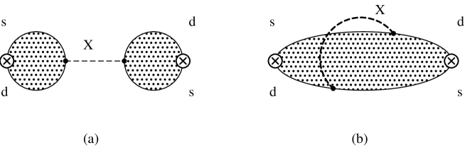
Figure 3: The leading, (a), and the non-factorizable next-to-leading in $1/N_{c}$, (b), corrections to the $\Delta S=2$ two-point function $\Pi_{\Delta S=2}(q^{2})$ and thus to $B_{K}$. The shaded regions are planar QCD diagrams. The crosses are insertions of the pseudoscalar current, $P^{ds}(x)$.

The dotted regions are a single quark line filled with leading in $1/N_{c}$ gluon exchanges, a planar diagram. At the next-to-leading order in this expansion there are two classes of diagrams. One is the same as in Fig. 3a but now there is a non-planar contribution or an extra fermion loop inside each shaded region. These we call factorizable $1/N_{c}$ corrections. The second class is the diagram shown in Fig. 3b. Here the shaded region is filled with gluons in a planar fashion. It is this nontrivial class that we will compute in this paper. The first class can be calculated completely in Chiral Perturbation Theory. They provide the corrections needed to obtain the physical values of $F_{K}$, $m_{K}$ and wave function renormalization. All off-shell corrections needed here are also purely determined by the strong interaction CHPT coefficients.

Now we would like to give some arguments in favour of the technique we will use. The calculation of the hadronic matrix element in Eq. (1.5) involves the mastering of strong interactions at all energies between two very different scales, namely, the $W$ boson mass and the kaon mass. This is, of course, where the complexity of the calculation arises. Both the quark-gluon momenta and the $X$-boson momentum cover this broad range of energies. While we can use the asymptotic freedom of QCD to perform a perturbative expansion for energies large enough, we do not know yet how to do a QCD calculation below energies around a few GeV. The technique we want to use here is essentially the one used by Bardeen, Buras and Gérard in Ref.[10, 14] in a slightly different notation and making emphasis in the low-energy model to describe the strong interactions. We want to impose as many as possible QCD relations on this low-energy model (Weinberg Sum Rules and similar relations). More comments on which low-energy model we will use and why are in Section 5.

The crucial point in this approach is that in electroweak matrix elements while we cannot keep track of the quark-gluon momenta due to confinement, we can keep track of the scale of the operator by looking at the $X$-boson momentum. The same rôle is played by the photon in the $\pi^{+}-\pi^{0}$ mass difference case[22, 23, 24]. Looking again at the diagrams in Fig. 2 and equation (2.3), one can convince oneself that the scale dependence imposed by the running of the quark-gluon momenta at these energies can be identified with the dependence on the QCD renormalization scale under some conditions. First, for the diagrams in Fig. 2 one can see that by attaching gluon lines to the quark lines that the dependence in a $X$-boson cut-off can be identified up to corrections of order $q^{2}/\mu^{2}$ with the dependence on the gluon cut-off for these diagrams. Here $q^{2}$ denotes a typical external momentum coming through the quarks. The requirement of $q^{2}/\mu^{2}$ to be small is also the requirement that the operator product expansion is still valid at the scale $\mu$. Otherwise higher dimension operators are needed to be included in the QCD running to take care of the effects of external momenta. Of course, these would be the only corrections if the gluon propagator had the perturbative behaviour at all scales. This we know is not the case and is the reason why we have to go to an effective model at scales below the chiral symmetry breaking scale $\Lambda_{\chi}$. The hope is then that this effective model is sufficiently accurate up to a scale $\mu\leq\Lambda_{\chi}$ where both $q^{2}/\mu^{2}$ is small and the perturbative evolution has set in. In that case a matching between the change in the perturbative part and the change in the low-energy part with $\mu$ should appear for some scale between $q^{2}$ and $\Lambda_{\chi}^{2}$.

We will work in the Euclidean domain where all momenta squared are negative. Then, the integral in the modulus of the momentum $r$ in (2.3) is split into two parts,

$${}\int_{0}^{M_{W}}{\rm d}\,|r|=\int_{0}^{\mu}{\rm d}\,|r|+\int_{\mu}^{M_{W}}{\rm d}\,|r|\ .$$ (2.4)

In principle one should then evaluate both parts separately as was done for the $\pi^{+}-\pi^{0}$ mass difference in the above quoted references. Notice that from the diagrams for four-quark operators at quark-gluon level with just one-gluon line attached (i.e. order $\alpha_{s}$), can only generate logarithmically divergent terms in a cut-off $\mu$ of the gluon momentum. One expects that the same behaviour will appear from the low-energy part of the integral in Eq. (2.4) for some scale $\mu^{2}$ between $q^{2}$ and $\Lambda_{\chi}^{2}$, as discussed before, when the hadronic interactions are included to all orders in momenta. Therefore, here, we will do the upper part of the integral using the renormalization group (RG) using the identification of the scale dependence discussed above.

An alternative way of looking at this is to assume that at some intermediate scale $\mu$ we get from the low-energy calculation

$${}\Gamma_{\Delta S=2}(\mu)=-G_{F}{\displaystyle\int^{\mu}_{0}}\frac{\displaystyle{\rm d}^{4}r}{\displaystyle(2\pi)^{4}}\int{\rm d}^{4}x_{1}\,\int{\rm d}^{4}x_{2}\,e^{-ir\cdot(x_{2}-x_{1})}\,L^{sd}_{\mu}(x_{1})\,L_{sd}^{\mu}(x_{2})\,.$$ (2.5)

In QCD, the operator $\Gamma_{\Delta S=2}(\mu)$ obeys the following inhomogeneous renormalization group equation

$${}\mu\,\frac{\displaystyle{\rm d}\Gamma_{\Delta S=2}(\mu)}{\displaystyle{\rm d}\mu} = -\gamma_{\Delta S=2}(\mu)\,\Gamma_{\Delta S=2}(\mu)$$

$$= -\left[\gamma_{\Delta S=2}^{(1)}\frac{\alpha_{s}^{(1)}}{\pi}(\mu)+{\cal O}\left(\left(\frac{\alpha_{s}}{\pi}\right)^{2}\right)\right]\Gamma_{\Delta S=2}(\mu)\,,$$

$$\gamma_{\Delta S=2}^{(1)} = \frac{3}{2}\left(1-\frac{1}{N_{c}}\right)\,,$$ (2.6)

with $\gamma_{\Delta S=2}$ the gamma function of ${\cal O}_{\Delta S=2}(x)$ [5] and $\alpha_{s}^{(1)}$ the strong coupling constant to one-loop. This change corresponds to doing the integral in (2.5) from $\mu$ to $\mu+{\rm d}\mu$. Integrating then equation (2) between the scales $\mu$ and $M_{W}$, one gets the full integral of (2.3) to be the same but integrated up to $\mu$ and multiplied by $C(\mu)$, with $C(\mu)$ the corresponding Wilson coefficient. Therefore,

$${}\Gamma_{\Delta S=2}=-G_{F}\,C(\mu)\int_{0}^{\mu}\frac{d^{4}r}{(2\pi)^{4}}\int d^{4}x_{1}\int d^{4}x_{2}\,e^{-ir\cdot(x_{2}-x_{1})}L^{sd}_{\mu}(x_{1})L_{sd}^{\mu}(x_{2})$$ (2.7)

A strict analysis in $1/N_{c}$ would correspond to set $C(\mu)=1+d(\mu)\alpha_{s}^{(1)}(\mu)$ and evaluate the second term using factorization in leading $1/N_{c}$. $d(\mu)$ is what the one-gluon exchange diagrams would give with a lower cut-off $\mu$. We will, however, use the full one-loop Wilson coefficient $C(\mu)=\left(\alpha_{s}^{(1)}(\mu)/\alpha_{s}^{(1)}(M_{W})\right)^{a_{+}}$. Equation (2.7), is in fact the equivalent of the effective Hamiltonian in Eq. (1.3). The definition of the function ${\cal F}$ includes the factor $\alpha_{s}(M_{W})^{-a_{+}}$ from the Wilson coefficient $C(\mu)$. This permits, then, the identification of $B_{K}(\mu)$.

The basic difference here with respect to the $m_{\pi^{+}}^{2}-m_{\pi^{0}}^{2}$ case is two-fold. First the matrix element considered here has anomalous dimensions. It makes the identification of the scale dependence with the cut-off in the $X$-boson momentum highly nontrivial. We know that there should be an explicit logarithmic $\mu$ dependence here. In the $\pi^{+}-\pi^{0}$ mass difference case the matching was of order $1/\mu^{2}$ which means that the intermediate momentum regime is less important. The second difference is that in the $\pi^{+}-\pi^{0}$ case the mass difference can be related to a vacuum matrix element[25]. Here this is not possible. So while in the other case two-point functions were sufficient we now need to calculate four-point functions in the strong interactions. The contribution to the $K^{0}-\bar{K}^{0}$ matrix element vanishes in the chiral limit. This, together with the fact that the typical scale is the kaon mass makes that the effects of a nonzero quark mass are essential here . Thus one can only expect matching of the $\mu$ dependence in the $B_{K}$ case (if any) for scales where the effects of $nonzero$ quark masses are small, i.e. for scales $\mu$ larger than $m_{K}$ .

Up to now, we did not need to specify the low-energy model for the strong interactions. In Ref. [10], CHPT was used, however the range of applicability of CHPT is precisely below where one can expect a reasonable matching with QCD (i.e., above the kaon mass). Then, in Ref. [14] vector meson interactions were included using a particular VMD model, namely the Hidden Gauge Symmetry model. We will calculate the lower part of the integral by using an Extended Nambu–Jona-Lasinio (ENJL) cut-off model and also in CHPT as a test of our ENJL calculation. Some reasons for why do we believe this model is more suitable for this purpose and its advantages versus other choices are in Sect. 5. Here, we only want to point out that ENJL permits the control of chiral corrections. The chiral limit is not clear in other approaches when implementing VMD, for instance. As a matter of fact, a very important point we want to address in this analysis, is the effect of the explicit chiral symmetry breaking. In addition, this model allows also for an $1/N_{c}$ expansion and a chiral expansion like the one in CHPT (see Ref. [27]).

3 Chiral Perturbation Theory Calculation of $\Pi_{\Delta S=2}(q^{2})$

In this Section we study the $\Delta S=2$ two-point function $\Pi_{\Delta S=2}(q^{2})$ in Eq. (2.1) in the framework of Chiral Perturbation Theory; i.e we use CHPT to calculate the contribution of the strong interactions at low energies.

3.1 Lowest Order

At lowest order in the chiral expansion ${\cal O}(p^{2})$ [28] the strong interactions between the lowest pseudoscalar mesons including external vector, axial-vector, scalar and pseudoscalar sources is described by the following effective Lagrangian

$${\cal L}^{(2)}_{\rm eff}=\frac{F_{0}^{2}}{4}\left\{\mathrm{tr}\left(D_{\mu}UD^{\mu}U^{\dagger}\right)+\mathrm{tr}\left(\chi U^{\dagger}+U\chi^{\dagger}\right)\right\}$$ (3.8)

where $D_{\mu}$ denotes the covariant derivative

$${}D_{\mu}U=\partial_{\mu}U-i(v_{\mu}+a_{\mu})U+iU(v_{\mu}-a_{\mu})\,,$$ (3.9)

and $U\equiv\exp\left(\frac{i\sqrt{2}\Phi}{F_{0}}\right)$ an SU(3) matrix incorporating the octet of pseudoscalar mesons

$${}\Phi(x)=\frac{\vec{\lambda}}{\sqrt{2}}\vec{\phi}=\left(\begin{array}[]{ccc}\frac{\displaystyle\pi^{0}}{\displaystyle\sqrt{2}}+\frac{\displaystyle\eta_{8}}{\displaystyle\sqrt{6}}&\pi^{+}&K^{+}\\ \pi^{-}&-\frac{\displaystyle\pi^{0}}{\displaystyle\sqrt{2}}+\frac{\displaystyle\eta_{8}}{\displaystyle\sqrt{6}}&K^{0}\\ K^{-}&\overline{K}^{0}&-\frac{\displaystyle 2\eta_{8}}{\displaystyle\sqrt{6}}\end{array}\right)\,.$$ (3.10)

In Eq. (3.9) $v_{\mu}(x)$ and $a_{\mu}(x)$ are external 3 $\times$ 3 vector and axial-vector field matrices. In Eq. (3.8) $\chi\equiv 2B_{0}\left({\cal M}+s(x)+ip(x)\right)$ with $s(x)$ and $p(x)$ external scalar and pseudoscalar 3 $\times$ 3 field matrices and ${\cal M}$ the 3 $\times$ 3 flavour matrix ${\cal M}={\rm diag}(m_{u},m_{d},m_{s})$ which collects the light quark masses. The constant $B_{0}$ is related to the vacuum expectation value

$$\left.\langle 0|\bar{q}q|0\rangle\right|_{q=u,d,s}=-F_{0}^{2}B_{0}\left(1+{\cal O}({\cal M})\right)\,.$$ (3.11)

In this normalization, $F_{0}$ is the chiral limit value corresponding to the pion decay coupling $F_{\pi}\simeq 92.5$ MeV. In the absence of the $U(1)_{A}$ anomaly (large $N_{c}$ limit) [29], the SU(3) singlet $\eta_{1}$ field becomes the ninth Goldstone boson which is incorporated in the $\Phi(x)$ fields as

$${}\Phi(x)=\frac{\vec{\lambda}}{\sqrt{2}}\vec{\phi}+\frac{\eta_{1}}{\sqrt{3}}{\mbox{\large\bf 1}}\,.$$ (3.12)

The effective realization of the pseudoscalar current $P^{ds}(x)$ at low-energies can be obtained from the divergence of the $ds$ component the axial-vector quark current. Then,

$$P^{ds}(x)=\sqrt{2}\,F_{0}B_{0}\bar{K}^{0}+\cdots$$ (3.13)

where we have explicitly given the lowest order term. The operator $\Gamma_{\Delta S=2}$ transforms as a component of a (27_L, 1_R) tensor under SU(3)_L $\times$ SU(3)_R chiral rotations. The realization of this operator in terms of the relevant low-energy degrees of freedom is determined uniquely by its symmetry structure. At leading order in the $1/N_{c}$ expansion, this operator has the well-known factorizable current $\times$ current structure

$${}\Gamma_{\Delta S=2}^{1/N_{c}}=-G_{27}G_{F}\,{\displaystyle\int}{\rm d}^{4}y{\cal L}^{\mu}_{23}(y){\cal L}_{\mu 23}(y)$$ (3.14)

with ${\cal L}_{\mu}={\cal L}^{(1)}_{\mu}+{\cal L}^{(2)}_{\mu}+\cdots$ in an expansion in external momenta and quark masses. The lowest order is ${\cal L}^{(1)}_{\mu}=-i\frac{F_{0}^{2}}{2}U^{\dagger}D_{\mu}U$. The coupling $G_{27}$ is a scale independent quantity modulating the (27_L, 1_R) part under the SU(3)_L $\times$ SU(3)_R chiral rotations of the Standard Model Lagrangian. In the large $N_{c}$ limit $G_{27}=1$.

In fact, at lowest ${\cal O}(p^{2})$ in CHPT, the effective realization of the $\Gamma_{\Delta S=2}$ operator has the factorizable structure in Eq. (3.14) with ${\cal L}_{\mu}\to{\cal L}^{(1)}_{\mu}$. One can now perform the calculation of $\Pi_{\Delta S=2}(q^{2})$ at this order. The only diagram contributing at this order is (a) in Fig. 4.

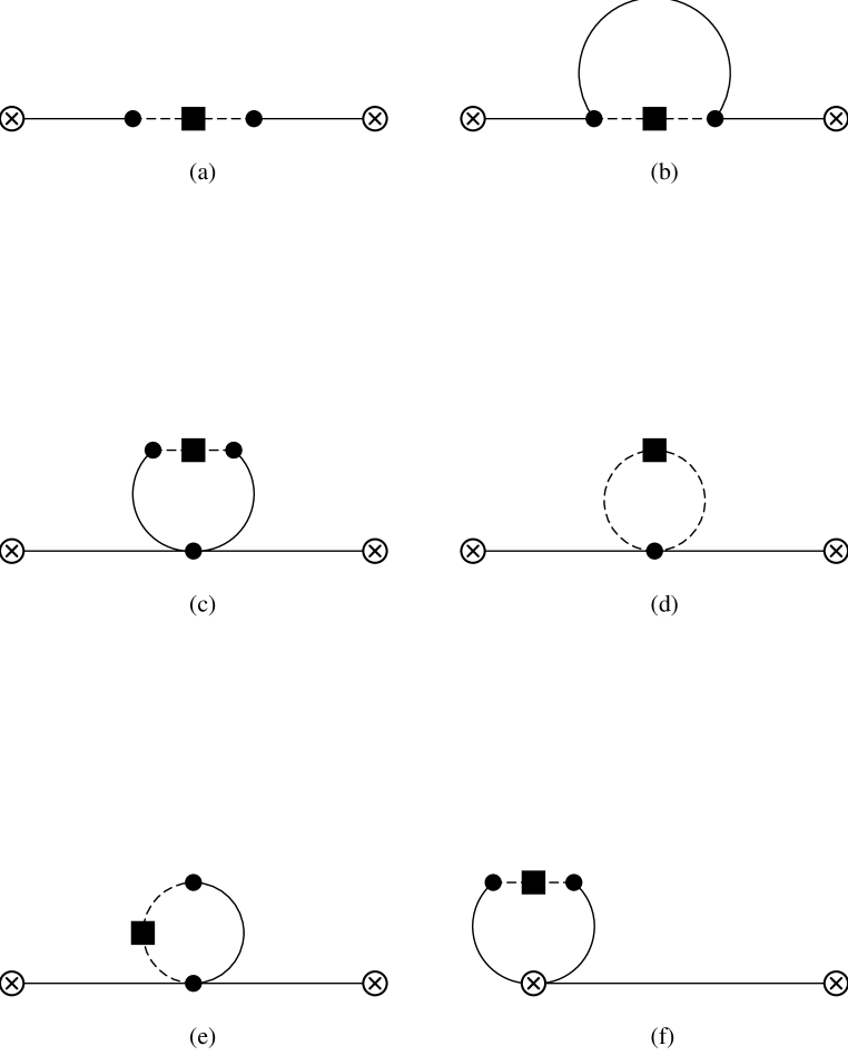
Figure 4: Chiral Perturbation Theory contributions to $\Pi_{\Delta S=2}(q^{2})$ (I) . (a) Lowest order. (b)-(f) Higher order non-factorizable. A circled cross is an insertion of the external pseudoscalar current, $P^{sd}(x)$, a dot is a strong interaction vertex and the square with the dashed lines to the dots represents the $\Delta S=2$ operator, $\Gamma_{\Delta S=2}$. The full lines are meson lines.

Then, we obtain

$${}\Pi_{\Delta S=2}(q^{2})=-\frac{2B_{0}^{2}F_{0}^{4}}{\left(q^{2}-m_{0}^{2}\right)^{2}}q^{2}G_{27}.$$ (3.15)

Where $m_{0}$ is the chiral limit value corresponding to the kaon mass. This result is equivalent to

$$\langle\bar{K}^{0}|{\cal O}_{\Delta S=2}(x)|K^{0}\rangle=m_{0}^{2}\,F_{0}^{2}g_{27}(\mu)\qquad{\rm or}\qquad\hat{B}_{K}^{(2)}=\frac{3}{4}G_{27}.$$ (3.16)

The coupling constant $g_{27}(\mu)$ is the overall factor modulating the (27_L, 1_R) representation of which the operator ${\cal O}_{\Delta S=2}(x)$ is a component. The relation between $G_{27}$ and $g_{27}(\mu)$ is $G_{27}\equiv g_{27}(\mu)\alpha_{s}(\mu)^{a_{+}}$.

3.2 Next-to-Leading Order

At ${\cal O}(p^{4})$ we have to consider both tree-level ${\cal O}(p^{4})$ counterterms and loops of the ${\cal O}(p^{2})$ terms. To define these loops one needs to introduce a subtraction point $\nu^{2}$. This is the CHPT subtraction scale and is not related to the scale $\mu$ used in the other sections. See the more extensive discussion in Sect. 4.

Let us first look at the pseudo-Goldstone boson loops. Here we will present both the results in the octet symmetry approximation, i.e. using the $U$ matrix in Eq. (3.10) with no $\eta_{1}$, and in the nonet symmetry approximation (or strict large $N_{c}$ limit); i.e. using the $U$ matrix in Eq. (3.12). First let us give the result for the octet symmetry case. The contributions from pseudo-Goldstone boson loops that are factorizable into two diagrams after cutting the propagator of the fictitious $\Delta S=2$ $X$-boson introduced in Sect. 2 can be reabsorbed in the corresponding ${\cal O}(p^{4})$ expressions for $m_{0}$, $B_{0}$, and $F_{0}$ in Eq. (3.15). They also give wave function renormalization. These are in Figs. (a), (b) and (c) in Fig. 5 (plus the symmetric ones).

In addition, there are also non-factorizable contributions from pseudo-Gold/-stone boson loops in Figs. (b), (c), (e), and (f) in Fig. 4, where the boxes are the $\Gamma_{\Delta S=2}$ operator at ${\cal O}(p^{2})$. The calculation of these loops gives the following results for $\Pi_{\Delta S=2}(q^{2})$. For the integrals we only give the $\overline{MS}$ renormalized finite part at some scale $\nu$. The diagram in Fig. (b) gives

$$i\frac{B_{0}^{2}F_{0}^{2}}{\left(q^{2}-m_{K}^{2}\right)^{2}}{\displaystyle\int}\frac{{\rm d}^{4}p}{(2\pi)^{4}}\frac{1}{2}(q+p)^{2}\left(\frac{1}{p^{2}-m_{\pi}^{2}}+\frac{3}{p^{2}-m_{\eta_{8}}^{2}}\right)$$ (3.17)

$$\doteq \frac{B_{0}^{2}F_{0}^{4}}{(q^{2}-m_{K}^{2})^{2}}\frac{1}{16\pi^{2}F_{0}^{2}}\,$$

$$\times \frac{1}{2}\left[(q^{2}+m_{\pi}^{2})m_{\pi}^{2}\ln(m_{\pi}^{2}/\nu^{2})+3(q^{2}+m_{\eta_{8}}^{2})m_{\eta_{8}}^{2}\ln(m_{\eta_{8}}^{2}/\nu^{2})\right].$$

For the sum of diagrams (c) and (f) plus the symmetric one, we get

$$i\frac{2}{3}\frac{B_{0}^{2}F_{0}^{2}}{\left(q^{2}-m_{K}^{2}\right)^{2}}\,{\displaystyle\int}\frac{{\rm d}^{4}p}{(2\pi)^{4}}\frac{p^{2}(p^{2}+3q^{2}-m_{K}^{2})}{\left(p^{2}-m_{K}^{2}\right)^{2}}$$

$$\doteq\frac{B_{0}^{2}F_{0}^{4}}{(q^{2}-m_{K}^{2})^{2}}\,\frac{1}{16\pi^{2}F_{0}^{2}}\frac{2}{3}m_{K}^{2}\left[(6q^{2}+m_{K}^{2})\ln\left(m_{K}^{2}/\nu^{2}\right)+3q^{2}\right].$$ (3.18)

Diagram (d) does not occur in pure CHPT. More about this diagram is in the Sects. 4 and 7. Diagram (e) gives

$$-i\frac{8}{3}\frac{B_{0}^{2}F_{0}^{2}}{\left(q^{2}-m_{K}^{2}\right)^{2}}{\displaystyle\int}\frac{{\rm d}^{4}p}{(2\pi)^{4}}\frac{p^{2}}{p^{2}-m_{K}^{2}}$$

$$\doteq-\frac{B_{0}^{2}F_{0}^{4}}{(q^{2}-m_{K}^{2})^{2}}\frac{1}{16\pi^{2}F_{0}^{2}}\,\frac{8}{3}m_{K}^{4}\ln(m_{K}^{2}/\nu^{2})$$ (3.19)

To this result one has to add ${\cal O}(p^{4})$ counterterms.

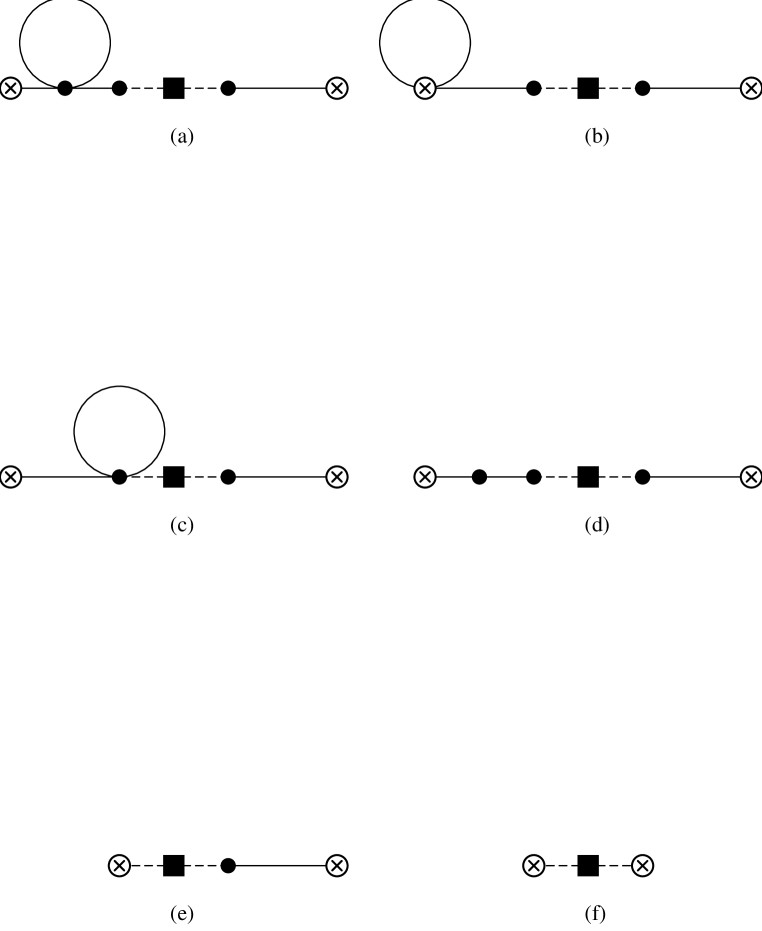
Figure 5: Chiral Perturbation Theory contributions to $\Pi_{\Delta S=2}(q^{2})$ (II) . (a)-(c) Factorizable loop corrections. (d)-(f) Counterterm contributions. Symbols are as in Fig. 4. See text for more explanation.

The counterterms of strong origin are factorizable. The corresponding diagrams are in Figs. (a) in Fig. 4 and (d) in Fig. 5, plus the symmetric ones. They can be completely calculated from the ${\cal O}(p^{4})$ chiral Lagrangian classified by Gasser and Leutwyler [30] in terms of the $L_{i}$, $i=1,\cdots 10$ and $H_{j}$, $j=1,2$ couplings. These corrections can be reabsorbed in the corresponding ${\cal O}(p^{4})$ expression for $m_{K}$ and wave function renormalization. In addition there are also ${\cal O}(p^{4})$ $\Delta S=2$ counterterms of weak origin. The corresponding diagrams are in Figs. (a) in Fig. 4, (e) and (f) in Fig. 5, plus the symmetric ones. The general structure of these operators was classified in Refs. [16, 17, 18]. Then the ${\cal O}(p^{4})$ $\Delta S=2$ structure of counterterms contributing to the $\Delta S=2$ two-point function $\Pi_{\Delta S=2}(q^{2})$ is

$${}\Gamma^{(4)}_{\Delta S=2} \doteq -G_{27}\,G_{F}\,{\displaystyle\int}{\rm d}^{4}y\left[D_{1}\,F_{0}^{4}\left(\chi^{\dagger}U+U^{\dagger}\chi\right)_{23}(y)\left(\chi^{\dagger}U+U^{\dagger}\chi\right)_{23}(y)\right.$$ (3.20)

$$+ D_{2}\,F_{0}^{4}\left(\chi^{\dagger}U-U^{\dagger}\chi\right)_{23}(y)\left(\chi^{\dagger}U-U^{\dagger}\chi\right)_{23}(y)$$

$$+ iD_{3}\,F_{0}^{2}\,{\cal L}^{(1)\mu}_{23}(y)\left(D_{\mu}\chi^{\dagger}U-U^{\dagger}D_{\mu}\chi\right)_{23}(y)$$

$$+ D_{4}\,{\cal L}^{(1)\mu}_{23}(y)\left\{\chi^{\dagger}U+U^{\dagger}\chi,{\cal L}^{(1)}_{\mu}\right\}_{23}(y)$$

$$+ iD_{5}\,{\cal L}^{(1)\mu}_{23}(y)\left[\chi^{\dagger}U-U^{\dagger}\chi,{\cal L}^{(1)}_{\mu}\right]_{23}(y)$$

$$+ D_{6}\left(\chi^{\dagger}U+U^{\dagger}\chi\right)_{23}(y)\left({\cal L}^{(1)}_{\mu}(y){\cal L}^{(1)\mu}(y)\right)_{23}$$

$$+ \left.D_{7}\,\mathrm{tr}\left(\chi^{\dagger}U+U^{\dagger}\chi\right)(y){\cal L}^{(1)\mu}_{23}(y){\cal L}^{(1)}_{\mu 23}(y)\right].$$

These ${\cal O}(p^{4})$ $\Delta S=2$ counterterms have also a factorizable part which can be obtained expanding the large $N_{c}$ expression in Eq. (3.14). These can be obtained from the corresponding ${\cal O}(p)$ and ${\cal O}(p^{3})$ terms of the left quark currents ${\cal L}_{\mu}$ in CHPT. Then at large $N_{c}$, $D_{4}=4L_{5}/F_{0}^{2}$ and $D_{7}=8L_{4}/F_{0}^{2}$ and all the other counterterms are zero. Here $L_{5}$ and $L_{4}$ are two of the ${\cal O}(p^{4})$ chiral Lagrangian in the strong sector [30]. These factorizable counterterms can once more be absorbed in the corresponding ${\cal O}(p^{4})$ expression for $F_{K}$. So altogether the factorizable counterterms of both strong and weak origin are the needed ones to cancel the (CHPT) scale dependence generated by the factorizable pseudo-Goldstone boson loops discussed above, so that the factorizable part is completely calculable and gives the result in Eq. (3.15) with $m_{0}\to m_{K}$, $F_{0}\to F_{K}$ and $(m_{d}+m_{s})B_{0}\to m_{K}^{2}$ .

Let us discuss the non-factorizable or next-to-leading $1/N_{c}$ order contributions. They will give the non-trivial contributions to $B_{K}$. Although the calculation can be performed in terms of the couplings $D_{i}$, $i=1,\cdots,7$; these couplings are unfortunately not known and therefore it is not possible to calculate $B_{K}$ to ${\cal O}(p^{4})$ within CHPT. Meanwhile these couplings are not available experimentally one can try to calculate them. To do that one needs dynamical information for which some QCD inspired model can be useful. The corresponding calculation in an effective action approach can be found in Ref. [19]. In the next sections we will use the technique and dynamical assumptions explained in Sect. 2 to obtain in the large $N_{c}$ limit these $D_{i}$-like couplings appearing to all orders in CHPT.

In the large $N_{c}$ limit we have that $D_{1}$, $D_{2}$, $D_{3}$, $D_{4}-4L_{5}/F_{0}^{2}$, $D_{5}$ $D_{6}$ and $D_{7}$ are ${\cal O}(1/N_{c})$.

Diagram (a) in Fig. 4 produces two kaon propagators and the result after subtracting the part that is reabsorbed in the factorizable or large $N_{c}$ contributions, is

$$2\frac{B_{0}^{2}F_{0}^{4}}{(q^{2}-m_{K}^{2})^{2}}G_{27}\,\left[16D_{1}^{r}(\nu^{2})\left(m_{K}^{2}-m_{\pi}^{2}\right)^{2}+16D_{2}^{r}(\nu^{2})m_{K}^{4}\right.$$

$$\left.-q^{2}\left[2\left(D_{7}^{r}(\nu^{2})-8\frac{L_{4}^{r}(\nu^{2})}{F_{0}^{2}}\right)\left(2m_{K}^{2}+m_{\pi}^{2}\right)+4\left(D_{4}^{r}(\nu^{2})-4\frac{L_{5}^{r}(\nu^{2})}{F_{0}^{2}}\right)m_{K}^{2}\right]\right].$$

Diagram (e) plus the symmetric one in Fig. 5 produces one kaon propagator and the result is

$$2\frac{B_{0}^{2}F_{0}^{4}}{q^{2}-m_{K}^{2}}G_{27}\,\,\left[32D_{2}^{r}(\nu^{2})m_{K}^{2}+4D_{3}^{r}(\nu^{2})q^{2}\right].$$ (3.22)

And diagram (f) in Fig. 5 gives no kaon propagators and the result is

$$32B_{0}^{2}F_{0}^{4}G_{27}\,D_{2}^{r}(\nu^{2}).$$ (3.23)

Where we have only written the $\overline{MS}$ finite part at some scale $\nu$ in terms of $D_{i}^{r}(\nu^{2})$ and $L_{i}^{r}(\nu^{2})$.

Summing up all the contributions, namely factorizable and non-factorizable, pseudo-Goldstone boson loops and counterterms, we get the following result for the full $\Pi_{\Delta S=2}(q^{2})$ to ${\cal O}(p^{4})$

$${}\Pi_{\Delta S=2}(q^{2}) = -2\frac{m_{K}^{4}F_{K}^{4}}{(m_{s}+m_{d})^{2}(q^{2}-m_{K}^{2})^{2}}G_{27}q^{2}$$ (3.24)

$$\times \left[1+\frac{m_{K}^{2}}{16\pi^{2}F_{0}^{2}}\left\{A\frac{m_{K}^{2}}{q^{2}}+B+C\frac{q^{2}}{m_{K}^{2}}\right\}\right].$$

With

$${}A = -16\,[16\pi^{2}F_{0}^{2}]D_{1}^{r}(\nu^{2})\,\left(1-\frac{m_{\pi}^{2}}{m_{K}^{2}}\right)^{2}+\ln(m_{K}^{2}/\nu^{2})$$

$$- \frac{1}{4}\frac{m_{\pi}^{4}}{m_{K}^{4}}\ln(m_{\pi}^{2}/\nu^{2})-\frac{3}{4}\frac{m_{\eta_{8}}^{4}}{m_{K}^{4}}\ln(m_{\eta_{8}}^{2}/\nu^{2}).$$

$$B = [16\pi^{2}F_{0}^{2}]\left\{2\left(D_{7}^{r}(\nu^{2})-8\frac{L_{4}^{r}(\nu^{2})}{F_{0}^{2}}\right)\,\left(2+\frac{m_{\pi}^{2}}{m_{K}^{2}}\right)\right.$$

$$+ \left.4\left(D_{4}^{r}(\nu^{2})+D_{3}^{r}(\nu^{2})-4\frac{L_{5}^{r}(\nu^{2})}{F_{0}^{2}}\right)\right\}$$

$$- \left[2\ln(m_{K}^{2}/\nu^{2})+\frac{1}{4}\frac{m_{\pi}^{2}}{m_{K}^{2}}\ln(m_{\pi}^{2}/\nu^{2})+\frac{3}{4}\frac{m_{\eta_{8}}^{2}}{m_{K}^{2}}\ln(m_{\eta_{8}}^{2}/\nu^{2})+1\right]\,.$$

$$C = -16\,[16\pi^{2}F_{0}^{2}]\left(D_{2}^{r}(\nu^{2})+\frac{D_{3}^{r}(\nu^{2})}{4}\right).$$ (3.25)

Each of these $A$, $B$ and $C$ terms must be separately scale independent. The divergent part of the ${\cal O}(p^{4})$ couplings in Eq. (3.20) was also determined in Ref. [16, 17, 18], with

$$D_{i}=D_{i}^{r}(\nu^{2})+\frac{\gamma_{i}}{16\pi^{2}F_{0}^{2}}\nu^{d-4}\left[\frac{1}{d-4}+\frac{1}{2}\left\{\gamma_{E}-\ln(4\pi)-1\right\}\right]$$ (3.26)

and $\gamma_{1}=-1/24$, $\gamma_{2}=0$, $\gamma_{3}=0$, $\gamma_{4}=3$, $\gamma_{5}=0$, $\gamma_{6}=-3/2$, $\gamma_{7}=1$. The corresponding divergent part of the ${\cal O}(p^{4})$ strong chiral Lagrangian were determined in [30] with

$$L_{i}=L_{i}^{r}(\nu^{2})+\frac{\Gamma_{i}}{16\pi^{2}}\nu^{d-4}\left[\frac{1}{d-4}+\frac{1}{2}\left\{\gamma_{E}-\ln(4\pi)-1\right\}\right]\,.$$ (3.27)

The ones we need are $\Gamma_{4}=1/8$ and $\Gamma_{5}=3/8$. These divergences precisely cancel the ones generated by the pseudoscalar meson loops leaving a scale independent quantity. In the large $N_{c}$ counting $A$, $B$ and $C$ are ${\cal O}(1)$. Notice that in the limit $m_{s}=m_{d}$ one gets $A=0$. This means that the subtraction constant $\Pi_{\Delta S=2}(0)$ vanishes when $m_{s}=m_{d}$. Here we have used the Gell-Mann–Okubo octet symmetry relation $3m_{\eta_{8}}^{2}=4m_{K}^{2}-m_{\pi}^{2}$. The exact cancellation of the $A$ term for equal quark masses ($m_{s}=m_{d}$) introduces an unknown error in present lattice quenched calculations which are done in this approximation.

From the explicit calculations one can also obtain that the singlet meson, $\eta_{1}$ does not contribute to $\Pi_{\Delta S=2}(q^{2})$, and thus to $B_{K}$. The relevant flavour degree of freedom in the zero-charge sector is $\left[\overline{d}d-\overline{s}s\right]$ which is octet. So only SU(3) breaking effects can be important. In order to estimate these we have also performed the calculation in the nonet symmetry approximation; i.e. using the $U$ matrix in Eq. (3.12). This is the strict large $N_{c}$ limit and is the one analogous to the calculation we shall do afterwards using the ENJL as low-energy hadronic model. Also, as in the ENJL model calculation, we have taken the $\bar{q}q$ states as basis for the states running in the loops and not the mesonic basis of the lowest pseudoscalar mesons, namely $\pi$, $K$ and $\eta$ mesons. This will change some of the scale dependence of the logarithms since the dynamical fields are not the same. In fact, from the calculation using nonet symmetry and $\bar{q}q$ states we get the same expression as in Eq. (3.24) but changing $m_{\eta_{8}}^{2(4)}\ln(m_{\eta_{8}}^{2}/\nu^{2})$ by $(2/3)\,(2\,m_{K}^{2}-m_{\pi}^{2})^{1(2)}\ln((2\,m_{K}^{2}-m_{\pi}^{2})/\nu^{2})$ and $m_{\pi}^{2(4)}\ln(m_{\pi}^{2}/\nu^{2})$ by $2m_{\pi}^{2(4)}\ln(m_{\pi}^{2}/\nu^{2})$. The exponent in brackets is for the change in $A$, the other one is for the change in $B$. We have used here that the $\overline{d}d$ meson has the same mass as the pion while the $\overline{s}s$ one has a mass $2m_{K}^{2}-m_{\pi}^{2}$. This produces that in this basis of fields the divergences are $\gamma_{1}=-1/8$ and the remaining ones the same as given above.

The different chiral logarithms in the octet case versus the nonet case for the $A$ and $B$ terms produces a numerical difference, which for a scale $\nu=m_{\rho}\simeq 0.77$ GeV, is

$$A_{\rm octet}=A_{\rm nonet}+0.36$$ (3.28)

and

$$B_{\rm octet}=B_{\rm nonet}+0.32\ .$$ (3.29)

Let us now go to the $B_{K}$ parameter itself. After reducing the $\Delta S=2$ two-point function above we get to ${\cal O}(p^{4})$

$$\hat{B}_{K}^{(4)} = \frac{3}{4}G_{27}\,\left[1+\frac{m_{K}^{2}}{16\pi^{2}F_{0}^{2}}\left\{A+B+C\right\}\right].$$ (3.30)

The difference obtained above for the $A$ and $B$ terms from the chiral logarithms in the octet case versus the nonet case enlarge $\hat{B}_{K}^{(4)}$ by 0.09 in the octet case, i.e. no $\eta_{1}$.

3.3 Large $N_{c}$ expansion

In this subsection we would like to perform also an $1/N_{c}$ discussion in the framework of CHPT without additional dynamical assumptions. As said before in the large $N_{c}$ limit the $\Gamma_{\Delta S=2}$ operator has the factorizable structure in Eq. (3.14). We also know that in the large $N_{c}$ limit $G_{27}=1$. So to all orders in CHPT and leading $1/N_{c}$

$${}\hat{B}_{K}=\frac{3}{4}\,.$$ (3.31)

The next-to-leading order $1/N_{c}$ corrections to this result are more involved. At lowest order CHPT ${\cal O}(p^{2})$ one still has only the factorizable structure at next-to-leading ${\cal O}(1/N_{c})$ when substituting ${\cal L}_{\mu}$ by ${\cal L}_{\mu}^{(1)}$ in Eq. (3.14). This happens to all orders in $1/N_{c}$ and lowest ${\cal O}(p^{2})$. Now $G_{27}$ contains $1/N_{c}$ corrections. Then to ${\cal O}(p^{2})$ and to all orders in the $1/N_{c}$ expansion

$$\hat{B}_{K}^{(2)}=\frac{3}{4}G_{27}.$$ (3.32)

Donoghue et al. [6] used SU(3) chiral symmetry to estimate $G_{27}$ from the measured $K^{+}\to\pi^{+}\pi^{0}$ $\Delta I=3/2$ decay rate which is modulated by the same $G_{27}$. They estimated it to be

$${}G_{27}\simeq 0.88\frac{F_{0}^{2}}{F_{K}^{2}}\simeq 0.49$$ (3.33)

and

$${}B_{K}^{(2)}\simeq 0.37\,.$$ (3.34)

These two results above in (3.31) and (3.34) are quite well established. Now, one can go to ${\cal O}(p^{4})$ and next-to-leading $1/N_{c}$. Again one has the factorizable contributions that are reabsorbed in the values of $F_{K}$, $m_{K}$ and in wave function renormalization. But at this ${\cal O}(p^{4})$, there are also non-factorizable $1/N_{c}$ corrections. The result at next-to-leading ${\cal O}(1/N_{c})$ can be obtained from the previous section,

$$\hat{B}_{K}^{(4)} = \frac{3}{4}\,\left[G_{27}+\frac{m_{K}^{2}}{16\pi^{2}F_{0}^{2}}\left\{A+B+C\right\}\right].$$ (3.35)

Where now $G_{27}$ contains $1/N_{c}$ corrections and the $A$, $B$ and $C$ terms have the same expression but calculated to ${\cal O}(1)$ in the large $N_{c}$.

From the $A$, $B$ and $C$ terms one can see that there are five structures of counterterms to be determined. Namely, $G_{27}$, $D_{1}^{r}$, $D_{7}^{r}-8L_{4}^{r}/F_{0}^{2}$, $D_{4}^{r}+D_{3}^{r}-4L_{5}^{r}/F_{0}^{2}$ and $D_{2}^{r}+D_{3}^{r}/4$ To do that we need dynamical information on the strong interactions. In the next section we will see how they can be determined in the approach explained in Sect. 2 using CHPT to next-to-leading order. Then, in Sect. 8 we will use the full ENJL to obtain the low-energy contribution to the $\Gamma_{\Delta S=2}(\mu)$ function. There, the dynamical assumptions are both in the use of the ENJL model and in the identification of the cut-off scale $\mu$ with the perturbative renormalization scale. We are in this case calculating the $\Delta S=2$ two-point function at next-to-leading order in the $1/N_{c}$ expansion and to all orders in CHPT. So, we are in fact calculating all the $D_{i}$-like counterterms that appear to all orders in CHPT at leading ${\cal O}(1/N_{c})$.

Let us now sketch how this can be done to ${\cal O}(p^{4})$. In the chiral limit there are two counterterms

$${}G_{27}\hskip 56.9055pt{\rm and}\hskip 56.9055ptC=D_{2}^{r}+\frac{D_{3}^{r}}{4}\,.$$ (3.36)

In the chiral limit and on-shell there is only $G_{27}$. Then we can obtain $G_{27}$ from the chiral limit for $q^{2}=0$. The slope in this case will give the $C$ term. Outside the chiral limit there are three more structures to be determined. These can be determined due to their different $q^{2}$ behaviour. The $A$ term produces a pole in the $B_{K}(\mu^{2},q^{2})$ form factor at $q^{2}=0$ for $m_{d}\neq m_{s}$. From its residue on can solve for the $D_{1}$ counterterm. The $B$ term has two possible structures involving $D_{7}$ and $D_{4}$ respectively, that can be disentangled from the different $m_{\pi}^{2}/m_{K}^{2}$ dependence multiplying them.

In Sect. 8 we will see how an analogous discussion can be done to all orders in CHPT. There we will first determine the $G_{27}$ coupling by going to the chiral limit and making a numerical fit to to the ratio between the lowest order to the next-to-leading $1/N_{c}$ order to a polynomial in powers of $q^{2}$ starting by $q^{0}$. Then $G_{27}$ is the term at $q^{2}=0$. Once we have $G_{27}$, we do both, for the case of degenerate quarks $m_{s}=m_{d}$ and the real case $m_{s}\neq m_{d}$, another numerical fit to the ratio between the lowest order to the next-to-leading $1/N_{c}$ order to a polynomial in powers of $q^{2}$ starting in $q^{-2}$. Here, we are determining the $A$, $B$, $C$, $\ldots$ terms; i.e. the $D_{i}$-like counterterms.

We have one more general result in CHPT. To next-to-leading order in $1/N_{c}$ but to all orders in CHPT the diagrams that can contribute are still those depicted in Figs. 4 and 5. The vertices now are the ones appearing in the CHPT Lagrangian at all orders. There is still no non-analytic dependence on $q^{2}$ possible even with all possible vertices. The result from the previous section that at order $p^{4}$ the dependence on $q^{2}$ in $\Pi_{\Delta S=2}$ is analytic, is thus true to all orders up to next-to-leading order in $1/N_{c}$.

4 Chiral Perturbation Theory Calculation in the $1/N_{c}$ Expansion

In this section we use CHPT to estimate the low-energy contribution to $\Gamma_{\Delta S=2}(\mu)$ in Eq. (2.5). We will only discuss the nonet symmetry case and using the states $\bar{q}q$ as dynamical basis for the states running in the loops as explained in the previous section. As said in Section 2 at some intermediate energy region we want to identify the dependence on a cut-off $\mu$ in the $X$-boson momentum with the QCD renormalization scale dependence. Under the conditions explained there, one expects it to be plausible for some value below the spontaneous symmetry breaking scale.

This scale $\mu$ is thus not related to the scale $\nu$ of the previous section, even though it appears in a similar fashion in the logarithms. If we wanted to extend the analysis presented here going beyond the lowest order in CHPT coupling of currents to the mesons a similar scale $\nu$ would appear. This would then cancel the dependence on $\nu$ of the $L_{i}$ in the higher order CHPT Lagrangian. The answer then would be $\nu$ independent. The scale $\mu$ is the upper limit of the integral in Eq. (2.5) and would still be present.

We have chosen to route the momentum in the loop integrals $r$ as $p_{X}=r+q$ where $p_{X}$ is the $X$-boson momentum and $q$ is the external momentum. Any other routing will induce similar uncertainties of ${\cal O}(q^{2}/\mu^{2})$. Then, we do these integrals in the Euclidean space cutting-off the loop momentum $r_{E}$ for $|r_{E}|^{2}>\mu^{2}$ (where the subscript $E$ stands for Euclidean).

We want to emphasize here that this is not a pure CHPT calculation as in Section 3. It contains some dynamical assumptions like that we can reproduce the QCD renormalization scale dependence in the $1/N_{c}$ expansion with a cut-off in the $X$-boson momentum, i.e. that lowest order CHPT is good enough up to a scale $\mu$ where we can compare with the perturbative part of the calculation. We will make then both an expansion in $q^{2}/\Lambda_{\chi}^{2}$, $\mu^{2}/\Lambda_{\chi}^{2}$ and quark masses over the same scale $\Lambda_{\chi}^{2}$ in the context of an $1/N_{c}$ expansion. $\Lambda_{\chi}\simeq 1.2$ GeV is the scale of spontaneous symmetry breaking. In the previous section the requirement was $q^{2}/\Lambda_{\chi}^{2}$ and $m_{K}^{2}/\Lambda_{\chi}^{2}$ small.

In addition to being an estimate of the non-leptonic parameters in the sense of Ref. [10], CHPT provides a model independent result that will help us to check our ENJL calculation for $q^{2}/\Lambda_{\chi}^{2}$ and $\mu^{2}/\Lambda_{\chi}^{2}$ small enough.

In this notation of CHPT the QCD quark current $P^{ds}(x)$ couples to the external source $[p(x)]_{23}$ and the left current $L_{\mu}^{sd}(x)$ to $[v_{\mu}(x)-a_{\mu}(x)]_{32}$.

At lowest order in the chiral expansion only the factorizable diagram in Fig. 4 contributes. This contribution is ${\cal O}(N_{c}^{2})$ in the $1/N_{c}$ expansion. The result is

$${}-\frac{2B_{0}^{2}F_{0}^{4}}{\left(q^{2}-m_{0}^{2}\right)^{2}}\,q^{2}\,.$$ (4.1)

This result when properly reduced is equivalent to

$$\langle\overline{K}^{0}|{\cal O}_{\Delta S=2}(x)|K^{0}\rangle=m_{0}^{2}F_{0}^{2}.$$ (4.2)

At the next order we have both factorizable ${\cal O}(N_{c}^{2})$ and non-factorizable ${\cal O}(N_{c})$ contributions. The ones that are factorizable are given in terms of the couplings of the ${\cal O}(p^{4})$ chiral Lagrangian which was classified by Gasser and Leutwyler and loops of the ${\cal O}(p^{2})$ chiral Lagrangian. These are completely calculable and we do not need any dynamical assumption, they only involve momenta of order $q^{2}$ and not of order $\mu^{2}$. These corrections are precisely the ones that redefine the $B_{0}^{2}F_{0}^{4}$ couplings to its ${\cal O}(p^{4})$ expressions and are shown in Fig. (a) in Fig. 4 and Figs. (a) to (d) plus the symmetric ones in Fig. 5. Those that are non-factorizable are shown in Figs. (b) to (f) plus the symmetric ones in Fig. 4.

Diagram (b) in Fig. 4 gives the following contribution

$${}-\frac{B_{0}^{2}F_{0}^{2}}{(q^{2}-m_{K}^{2})^{2}}{\displaystyle\int^{\mu}}\frac{{\rm d}^{4}r_{E}}{(2\pi)^{4}}\,(r_{E}-q_{E})^{2}\left[\frac{\displaystyle 1}{\displaystyle r_{E}^{2}+m_{\pi}^{2}}+\frac{\displaystyle 1}{\displaystyle r_{E}^{2}+2m_{K}^{2}-m_{\pi}^{2}}\right]$$

$$=-\frac{B_{0}^{2}F_{0}^{4}}{(q^{2}-m_{K}^{2})^{2}}\,\frac{1}{16\pi^{2}F_{0}^{2}}\,\left[\mu^{4}-(q^{2}+m_{\pi}^{2})\left(\mu^{2}-m_{\pi}^{2}\ln\left(\frac{\mu^{2}-m_{\pi}^{2}}{m_{\pi}^{2}}\right)\right)\right.$$

$$\left.-(q^{2}+2m_{K}^{2}-m_{\pi}^{2})\left(\mu^{2}-\left(2m_{K}^{2}-m_{\pi}^{2}\right)\ln\left(\frac{\mu^{2}+2m_{\pi}^{2}-m_{\pi}^{2}}{2m_{K}^{2}-m_{\pi}^{2}}\right)\right)\right]\,.$$ (4.3)

Keep in mind that the mass of the $\overline{s}s$ state is $2m_{K}^{2}-m_{\pi}^{2}$.

The sum of diagrams (c) and (f) plus the symmetric one in Fig. 4 gives

$$-\frac{2}{3}\,\frac{B_{0}^{2}F_{0}^{2}}{(q^{2}-m_{K}^{2})^{2}}{\displaystyle\int^{\mu}}\frac{{\rm d}^{4}r_{E}}{(2\pi)^{4}}\,\frac{(r_{E}+q_{E})^{2}\left[3q_{E}^{2}+(r_{E}+q_{E})^{2}+m_{K}^{2}\right]}{\left((r_{E}+q_{E})^{2}+m_{K}^{2}\right)^{2}}$$

$$= -\frac{B_{0}^{2}F_{0}^{4}}{(q^{2}-m_{K}^{2})^{2}}\,\frac{1}{16\pi^{2}F_{0}^{2}}$$

$$\times \frac{2}{3}\,\left[\frac{\mu^{4}}{2}-\left(3q^{2}+m_{K}^{2}\right)F_{1}(\mu^{2},q^{2},m_{K}^{2})+3q^{2}m_{K}^{2}F_{2}(\mu^{2},q^{2},m_{K}^{2})\right]$$

$$=_{\displaystyle m_{K}^{2}\to 0} -\frac{B_{0}^{2}F_{0}^{4}}{(q^{2}-m_{K}^{2})^{2}}\,\frac{1}{16\pi^{2}F_{0}^{2}}\frac{1}{3}\left[\mu^{4}-6q^{2}\mu^{2}-3q^{4}\right]$$

$$=_{\displaystyle q^{2}\to 0} -\frac{B_{0}^{2}F_{0}^{4}}{(q^{2}-m_{K}^{2})^{2}}\,\frac{1}{16\pi^{2}F_{0}^{2}}\frac{1}{3}\left[\mu^{4}-2m_{K}^{2}\left(\mu^{2}-m_{K}^{2}{\rm ln}\left(\frac{\mu^{2}+m_{K}^{2}}{m_{K}^{2}}\right)\right)\right]\ .$$

The functions $F_{1}$ and $F_{2}$ are

$$F_{i}(\mu^{2},q^{2},m_{K}^{2})=\int_{0}^{\mu^{2}}{\rm d}s\frac{1}{2q^{2}}\lambda^{2-i}\,\left[1-\frac{s+m_{K}^{2}-q^{2}}{\lambda}\right]\ ,$$ (4.5)

using $\lambda=\sqrt{(s+m_{K}^{2}-q^{2})^{2}+4sq^{2}}$. These integrals can be performed analytically but the result is very cumbersome. The final two lines in Eq. (LABEL:seconddiag) give the expressions for $m_{K}^{2}=0$ and $q^{2}=0$, respectively.

Diagram (d) in Fig. 4 gives no contribution at this order. This diagram deserves more attention related with the Fierzed terms [21]. It provides in fact another non-trivial check. In the soft pion limit, one can relate the VV (AA) part of this diagram with a sum rule to some moment of a VV-AA two-point function [31]. These issues are discussed in Section 7.

Diagram (e) in Fig. 4 gives

$${}\frac{8}{3}\frac{B_{0}^{2}F_{0}^{2}}{(q^{2}-m_{K}^{2})^{2}}{\displaystyle\int^{\mu}}\frac{{\rm d}^{4}r_{E}}{(2\pi)^{4}}\,\frac{(r_{E}+q_{E})^{2}}{(r_{E}+q_{E})^{2}+m_{K}^{2}}$$

$$=\frac{B_{0}^{2}F_{0}^{4}}{(q^{2}-m_{K}^{2})^{2}}\frac{1}{16\pi^{2}F_{0}^{2}}\frac{8}{3}\left[\frac{\mu^{4}}{2}-m_{K}^{2}F_{1}(\mu^{2},q^{2},m_{K}^{2})\right]$$

$$\doteq\frac{B_{0}^{2}F_{0}^{4}}{(q^{2}-m_{K}^{2})^{2}}\frac{1}{16\pi^{2}F_{0}^{2}}\frac{8}{3}\left[\frac{\mu^{4}}{2}-m_{K}^{2}\left(\mu^{2}-m_{K}^{2}\ln\left(\frac{\mu^{2}+m_{K}^{2}}{m_{K}^{2}}\right)\right)\right]\,.$$ (4.6)

The result in the last line above is exact both for $q^{2}=0$ and for $m_{K}^{2}=0$.

The quartic dependence in the cut-off cancels between the different diagrams as required by chiral symmetry. The $1/N_{c}$ expansion and the dynamical assumptions mentioned above have allowed us to make a full calculation of the two-point function $\Pi_{\Delta S=2}(q^{2})$ both at next-to-leading ${\cal O}(N_{c})$ in the $1/N_{c}$ expansion and ${\cal O}(p^{4})$ in the chiral expansion. The factorizable loops have a $\nu$ dependence that cancels as explained in the beginning of this section. The integrals in (4), (LABEL:seconddiag) and (4) produce both analytical and non-analytical $\mu$-scale dependence. The cut-off procedure we followed has produced logarithmic dependence in $\mu$ for $B_{K}$ proportional to meson masses (see below). This dependence should cancel when the chiral expansion for $\Pi_{\Delta S=2}(q^{2})$ is considered to all orders giving no contribution to the running of $B_{K}(\mu)$ for large $\mu$. The perturbative running is after all independent of the quark masses. Lowest order CHPT as used here is expected to loose validity before we reach such scales.

Here, we are actually calculating the combination of counterterms and chiral logs in Eqs. (3.36) and (3.2). So in order to extract the values of the coupling constants we should compare the full expression for $\Pi_{\Delta S=2}(q^{2})$ in (3.24), with the one calculated here.

In the chiral case $m_{s}=m_{d}=0$ the calculation of the next-to leading order contribution to $\Pi_{\Delta S=2}(q^{2})$ can be written as (assuming $\mu^{2}>q^{2}$)

$${}\frac{B_{0}^{2}F_{0}^{4}}{\left(q^{2}-m_{K}^{2}\right)^{2}}\frac{1}{16\pi^{2}F_{0}^{2}}\left[4\mu^{2}q^{2}+q^{4}\right]\,.$$ (4.7)

This result added to the one in (4.1), then properly reduced and compared with the $B_{K}$ definition in Eq. (1.5) gives

$$B_{K}(\mu^{2},q^{2})=\frac{3}{4}\left(1-\frac{1}{16\pi^{2}F_{0}^{2}}\left[2\mu^{2}+\frac{q^{2}}{2}\right]\right).$$ (4.8)

As we already knew from the CHPT calculation in Sect. 3 there is no pole for this case. Doing now the general $m_{s}\neq m_{d}$ case we can get the $G_{27}$ coupling and the $A$, $B$ and $C$ terms. Then to next-to-leading order in $1/N_{c}$ and to order $p^{4}$, i.e. we have neglected the higher order CHPT terms in the last line in Eq. (LABEL:seconddiag),

$${}G_{27} = \alpha_{s}(\mu)^{a_{+}}-\frac{\mu^{2}}{8\pi^{2}F_{0}^{2}}$$

$$A = -\ln\left(\frac{\mu^{2}+m_{K}^{2}}{m_{K}^{2}}\right)+\frac{1}{2}\frac{m_{\pi}^{4}}{m_{K}^{4}}\ln\left(\frac{\mu^{2}+m_{\pi}^{2}}{m_{\pi}^{2}}\right)$$

$$+ \frac{1}{2}\left(2-\frac{m_{\pi}^{2}}{m_{K}^{2}}\right)^{2}\ln\left(\frac{\mu^{2}+2m_{K}^{2}-m_{\pi}^{2}}{2m_{K}^{2}-m_{\pi}^{2}}\right)$$

$$B = 2\ln\left(\frac{\mu^{2}+m_{K}^{2}}{m_{K}^{2}}\right)+\frac{1}{2}\frac{m_{\pi}^{2}}{m_{K}^{2}}\ln\left(\frac{\mu^{2}+m_{\pi}^{2}}{m_{\pi}^{2}}\right)$$

$$+ \frac{1}{2}\left(2-\frac{m_{\pi}^{2}}{m_{K}^{2}}\right)\,\ln\left(\frac{\mu^{2}+2m_{K}^{2}-m_{\pi}^{2}}{2m_{K}^{2}-m_{\pi}^{2}}\right)+{\cal O}\left(\frac{m_{K}^{2}}{\mu^{2}}\right).$$

$$C = -\frac{1}{2}+{\cal O}\left(\frac{m_{K}^{2}}{\mu^{2}}\right)\,.$$ (4.9)

Clearly the matching between the QCD perturbative scale dependence and the cut-off $\mu$ here in $G_{27}$, $A$, $B$ and $C$ is not good enough. Remember they have to be separately scale independent. To improve this situation we need to go to higher order in CHPT. This we will do in the next sections. Using an ENJL model as a good low-energy hadronic model we will calculate to all orders in CHPT in the framework of the $1/N_{c}$ expansion. This ${\cal O}(p^{4})$ will serve as a check of our ENJL calculation. In fact, the comparison of this result ($G_{27}$, $A$, $B$, and $C$) with the ENJL calculation for $q^{2}/\Lambda_{\chi}^{2}$ and $\mu^{2}/\Lambda_{\chi}^{2}$ small enough is good.

Taking the point of view of Ref. [10] we can compare Eqs. (4) and (3.2) to obtain

$$D_{1}^{r}(\nu^{2})=D_{7}^{r}(\nu^{2})-\frac{8L_{4}^{r}(\nu^{2})}{F_{0}^{2}} = 0\ ,$$

$$\left[16\pi^{2}F_{0}^{2}\right]\left(D_{4}^{r}(\nu^{2})+D_{3}^{r}(\nu^{2})-\frac{4L_{5}^{r}(\nu^{2})}{F_{0}^{2}}\right) = \frac{1}{4}\ ,$$

$$\left[16\pi^{2}F_{0}^{2}\right]\left(D_{2}^{r}(\nu^{2})+\frac{D_{3}^{r}(\nu^{2})}{4}\right) = \frac{1}{32}\ .$$ (4.10)

Notice that this assumes that for $\mu^{2}>>m_{K}^{2}$, this ${\cal O}(p^{4})$ calculation is enough to reproduce exactly the QCD perturbative scale dependence and thus one can choose $\mu=\nu$. This assumption, if good anywhere, would be good for scales $\mu$ around or below the spontaneous symmetry breaking scale ($\simeq 1.2$ GeV).

5 Short Description of the ENJL Model and its Connection with QCD

For recent comprehensive reviews on the NJL model [32] and the ENJL model [33], see Refs. [34, 35]. Here, we only will give a brief introduction and reasons why we choose this model. The QCD Lagrangian is given by

$${}{\cal L}_{\rm QCD} = {\cal L}^{0}_{\rm QCD}-\frac{1}{4}G_{\mu\nu}G^{\mu\nu}\,,$$

$${\cal L}^{0}_{\rm QCD} = \overline{q}\left\{i\gamma^{\mu}\left(\partial_{\mu}-iv_{\mu}-ia_{\mu}\gamma_{5}-iG_{\mu}\right)-\left({\cal M}+s-ip\gamma_{5}\right)\right\}q\,.$$ (5.1)

Here summation over colour degrees of freedom is understood and we have used the following short-hand notations: $\overline{q}\equiv\left(\overline{u},\overline{d},\overline{s}\right)$; $G_{\mu}$ is the gluon field in the fundamental SU(N_c) (N_c=number of colours) representation; $G_{\mu\nu}$ is the gluon field strength tensor in the adjoint SU(N_c) representation; $v_{\mu}$, $a_{\mu}$, $s$ and $p$ are external vector, axial-vector, scalar and pseudoscalar field matrix sources; ${\cal M}$ is the quark-mass matrix.

From lattice QCD numerical simulations, all indications are that in the purely gluonic sector there is a mass-gap. Therefore there seems to be a kind of cut-off mass in the gluon propagator (see the discussion in Ref. [36]). Alternatively one can think of integrating out the high-frequency (higher than $\Lambda_{\chi}$, a cut-off of the order of the spontaneous symmetry breaking scale) gluon and quark degrees of freedom and then expand the resulting effective action in terms of local fields. We then stop this expansion after the dimension six terms. This leads to the following effective action at leading order in the $1/N_{c}$ expansion

$${}{\cal L}_{\rm QCD} \rightarrow {\cal L}_{\rm ENJL}={\cal L}_{\rm QCD}^{\Lambda_{\chi}}+{\cal L}_{\rm ENJL}^{\rm S,P}+{\cal L}_{\rm ENJL}^{\rm V,A}+{\cal O}\left(1/\Lambda_{\chi}^{4}\right),$$ (5.2)

$${}{\rm with}\hskip 42.67912pt{\cal L}_{\rm ENJL}^{\rm S,P} = \frac{\displaystyle 8\pi^{2}G_{S}\left(\Lambda_{\chi}\right)}{\displaystyle N_{c}\Lambda_{\chi}^{2}}\,{\displaystyle\sum_{i,j}}\left(\overline{q}^{i}_{R}q^{j}_{L}\right)\left(\overline{q}^{j}_{L}q^{i}_{R}\right)$$ (5.3)

$${}{\rm and}\hskip 42.67912pt{\cal L}_{\rm ENJL}^{\rm V,P} = -\frac{\displaystyle 8\pi^{2}G_{V}\left(\Lambda_{\chi}\right)}{\displaystyle N_{c}\Lambda_{\chi}^{2}}\,{\displaystyle\sum_{i,j}}\left[\left(\overline{q}^{i}_{L}\gamma^{\mu}q^{j}_{L}\right)\left(\overline{q}^{j}_{L}\gamma_{\mu}q^{i}_{L}\right)+\left(L\rightarrow R\right)\right]\,.$$

Here $i,j$ are flavour indices and $\Psi_{R,L}\equiv(1/2)\left(1\pm\gamma_{5}\right)\Psi$. The couplings $G_{S}$ and $G_{V}$ are dimensionless and ${\cal O}(1)$ in the $1/N_{c}$ expansion and summation over colours between brackets is understood. The Lagrangian ${\cal L}^{\Lambda_{\chi}}_{\rm QCD}$ includes only low-frequency modes of quark and gluon fields. The remaining gluon fields can be assumed to be fully absorbed in the coefficients of the local quark field operators or alternatively also described by vacuum expectation values of gluonic operators. So at this level we have two different pictures of this model. One is where we have integrated out all the gluonic degrees of freedom and then expanded the resulting effective action in a set of local operators keeping only the first nontrivial terms in the expansion. In addition to this we can make additional assumptions. If we simply assume that these operators are produced by the short-range part of the gluon propagator we obtain $G_{S}=4G_{V}=N_{c}\alpha_{s}/\pi$. The two extra terms in (5.3) and (5) have however different anomalous dimensions so at the strong interaction regime where these should be generated there is no reason to believe this relation to be valid. In fact the best fit to the low energy effective chiral Lagrangians of ${\cal O}(p^{2})$ and ${\cal O}(p^{4})$ [37], is for $G_{S}\simeq 1.216\approx G_{V}\simeq 1.263$ (Fit 1 in Ref. [37]). The third parameter appearing in this picture is also obtained from the same fit, with $\Lambda_{\chi}=1.16$ GeV. The light quark masses in ${\cal M}$ are fixed then to obtain the physical pion and kaon masses in the poles of the pseudoscalar two-point functions [27]. Then we get $\overline{m}\equiv(m_{u}+m_{d})/2=3.2$ MeV and $m_{s}=83$ MeV.

The other picture is the one where we only integrate out the short distance part of the gluons and quarks. We then again expand the resulting effective action in terms of low-energy gluons and quarks in terms of local operators. Here we make the additional assumption that gluons only exists as a perturbation on the quarks. The quarks feel only the interaction with background gluons. This is worked out by only keeping the vacuum expectation values (VEVs) of gluonic operators and not including propagating gluonic interchanges. Most fits are in fact better with this gluonic VEV set to zero and when this is not so the results are quantitatively very close to the results in that case. Accordingly, we will take this gluonic VEV equal to zero in this work.

This model has the same symmetry structure as the QCD action at leading order in $1/N_{c}$ [38]. Notice that the $U(1)_{A}$ problem is absent at this order [29]. (For explicit symmetry properties under SU(3)_L $\times$ SU(3)_R of the fields in this model see reference [37].) The QCD chiral flavour anomaly can also be consistently reproduced in these kind of models when spin-1 four-fermion interactions are included [39]. In the chiral limit, this model (for $G_{S}>1$) breaks chiral symmetry spontaneously via an expectation value for the scalar quark-antiquark one-point function (quark condensate). We use here a cut-off in proper time as the regulator. In the mean-field approximation [10] we can introduce the vacuum expectation value into the Lagrangian, via an auxiliary field, and then keep only the terms quadratic in quark fields. The ${\cal L}_{\rm NJL}^{\rm S,P,V,A}$ above are then equivalent to a constituent chiral quark-mass term of the type in [40] of the form $-M_{Q}(\bar{q}_{L}U^{\dagger}q_{R}+\bar{q}_{R}Uq_{L})$ [41].

In this model, two-point functions are given by the general graph depicted in Fig. 6.

Figure 6: The graphs contributing to the two point-functions in the large $N_{c}$ limit. a) The class of all strings of constituent quark loops. The four-fermion vertices are either ${\cal L}^{\rm S,P}_{\rm ENJL}$ or ${\cal L}^{\rm V,A}_{\rm ENJL}$ in Eqs. (5.3) and (5). The crosses at both ends are the insertion of the external sources. b) The one-loop case.

How to sum these kind of strings of bubbles of constituent quarks for two-point functions, regularization independent relations obtained in this model, the extension of the technique from two-point to three-point functions including explicit chiral symmetry breaking, discussion of the Weinberg Sum Rules in this model, how VMD works in this model and more related phenomenological issues are treated in Refs. [24, 27, 37, 42] and reviewed in [35]. The general conclusion is that within its limitations the ENJL-type models do include a reasonable amount of the expected physics from QCD, its symmetries, their spontaneous breakdown and even some of its short distance information, as for instance the one embodied in the Weinberg Sum Rules. This is a very important point and has been one more of the reasons why we have chosen this model. Relations like the Weinberg Sum Rules are theorems of QCD and should be reproduced by any reasonable candidate to describe the low-energy dynamics. In fact, they are essential in the convergence of the hadronic contribution to the electromagnetic $\pi^{+}-\pi^{0}$ mass difference [25]. These relations guarantee the good matching between the low-energy behaviour and the high-energy one. Models to introduce vector fields like the Hidden Gauge Symmetry (HGS) do not always have this good intermediate behaviour. This HGS model was used in ref. [14] to estimate vector meson contributions to $B_{K}$ in an $1/N_{c}$ expansion.

The major drawback of the ENJL model is the lack of a confinement mechanism. Although one can always introduce an ad-hoc confining potential doing the job. We will smear the consequences of this drawback by working with internal and external momenta always Euclidean with $|p^{2}|<$ $\Lambda_{\chi}^{2}$. In the $1/N_{c}$ expansion, we will also only keep singlet color observables.

We will use the ENJL model as a model to fairly describe in the large $1/N_{c}$ limit the strong interactions between the lowest-lying mesons and, if needed, external sources. The model we are using is a tree-level loop model with a explicit cut-off regularization for one loop parts. This introduces the physical cut-off $\Lambda_{\chi}$. What we mean by a tree level loop model is the following. A general set of external fields is connected via a set of one-loop diagrams with three or more legs (vertices) and sums over connections of these vertices by a four-fermion interactions or a full chain like depicted in Fig. 6. These are also the contributions which are leading in $1/N_{c}$. Going beyond the tree-level approximation is going beyond the large $N_{c}$-limit. It is at this level that the hadronic properties of this model have been tested. Also to going beyond this one would have to include other operators not suppressed at the next-to-leading order in $1/N_{c}$ in the ENJL Lagrangian. At that level one also encounters the problem of regularizing overlapping divergences in the model. For the purpose we want to apply the model here, namely, for calculating next-to-leading $1/N_{c}$ corrections to hadronic matrix elements of four-quark operators to consider strings of bubbles is sufficient for the non-factorizable part, see Sect. 2. As discussed there the leading non-factorizable part is calculable by planar diagrams. This corresponds to the tree-level loop calculation.

6 The ENJL Calculation

In this Section we will explain how the calculation was done in the ENJL model. In the large $N_{c}$ limit there is just one kind of diagrams that can contribute. These are depicted in Fig. 7.

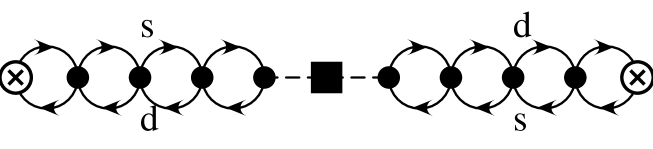
Figure 7: The leading $1/N_{c}$ contribution to $\Pi_{\Delta S=2}(q^{2})$ in the ENJL model. Symbols as in Fig. 3 except that a dot is now a ENJL-vertex in Eq. (5.2) and the full lines are constituent quark-lines. The box is a $\Gamma_{\Delta S=2}$ operator insertion. The flavour is mentioned next to the lines.

There the fermion lines are constituent quarks with mass $M_{d}$ and $M_{s}$ [27]. We have the product of two two-point functions, namely two mixed pseudoscalar–axial-vector $\Pi_{P}^{\mu}(q)_{sd}$. These two-point functions are connected by the exchange of a $X$-boson between the two left currents. At leading order in the $1/N_{c}$ expansion (i.e., at ${\cal O}(N_{c})$ in this case), each one of the two two-point functions are sum of all the strings of bubbles or loops, i.e. one, two, $\cdots$, $\infty$ . This type of diagrams factorizes when the $X$-boson propagator is cut. In terms of the two-point function[24, 27]

$$\Pi_{P}^{\mu}(q)_{sd}\equiv i\int{\rm d}^{4}x\,e^{iq\cdot x}\langle 0|T\left(A^{\mu}_{sd}(x)P_{ds}(0)\right)|0\rangle\,,$$ (6.1)

with $A^{\mu}_{sd}(x)\equiv\bar{s}(x)\gamma^{\mu}\gamma_{5}d(x)$, and $P_{ds}(x)\equiv\bar{d}(x)i\gamma_{5}s(x)$. Then, at leading order in $1/N_{c}$, we have

$${}\Pi_{\Delta S=2}(q^{2})=-\frac{1}{2}\Pi^{\mu}_{P}(-q)_{sd}\Pi_{\mu}^{P}(q)_{sd}\,.$$ (6.2)

The two-point function needed here was calculated in the full ENJL model, in the chiral limit in Ref. [24] and in Ref. [27] for non-zero quark masses. In both cases to all orders in the external momenta expansion. The result in Eq. (6.2) is equivalent to $B_{K}(\mu)=\hat{B}_{K}=3/4$ once $\Pi_{\Delta S=2}(q^{2})$ is reduced to the matrix element in Eq. (1.5).

At next-to-leading order in the $1/N_{c}$ expansion, we have two general kind of diagrams. The one depicted in Fig. 8 and the one in Fig. 9.

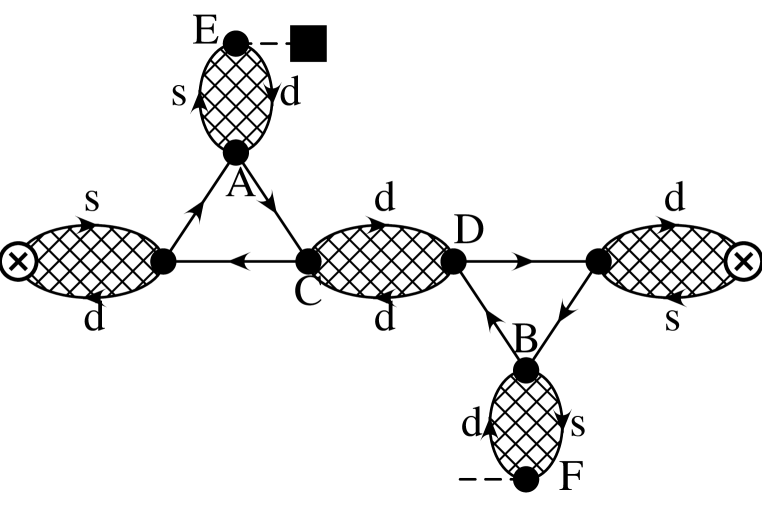
Figure 8: The class of three-point diagrams. Symbols as in Fig. 7, the hatched areas are a summation over sets of one-loop diagrams as shown in Fig. 6.

There is also the same type of diagram with the three-point functions tilted and the central propagator $\bar{d}d$ changed to $\bar{s}s$.

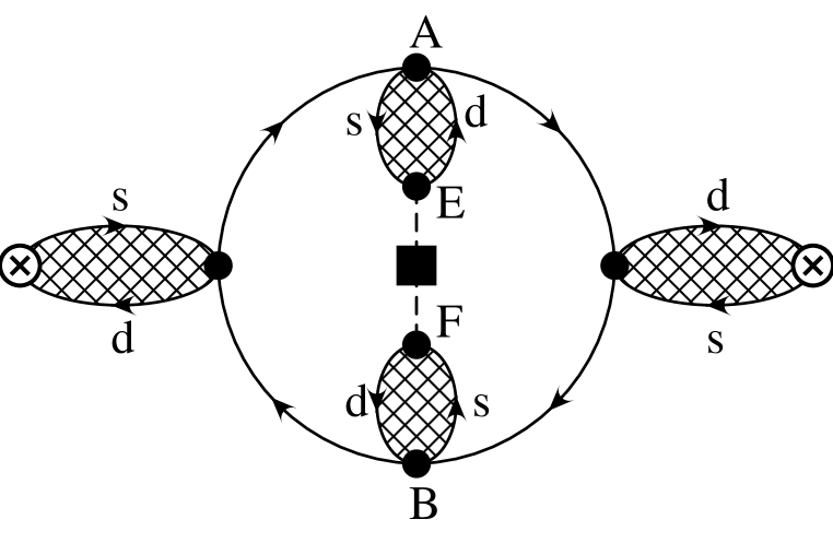
Figure 9: The class of four-point diagrams, symbols as in Fig. 8.

These are the two possibilities for the tree level loop diagrams and correspond to Fig. 3b. In both cases, when we cut the $X$-boson propagator, we have four external legs. Two connected to the left currents and the other two to the pseudoscalar sources. These are, then, tree-level constituent quark loop four-point functions. The diagram in Fig. 8 can be seen as the product of two one-loop three-point functions with a $P_{ds}$ pseudoscalar leg, a left current $L_{sd}^{\mu}$ leg and the third leg amputated. Then the two three-point functions are glued with a propagator, this can be $\bar{s}s$ or $\bar{d}d$ and with any kind of Dirac structure. The other class contains a one-loop four-point function dressed with two legs connecting the pseudoscalar sources $P_{ds}$ and another two connecting the left current sources $L^{\mu}_{sd}$. Therefore, we have to calculate in the ENJL model, at leading order in the $1/N_{c}$ expansion a generalized $\langle P^{ds}L_{sd}^{\mu}P^{ds}L^{sd}_{\mu}\rangle$ four-point function. This implies the actual calculation of many one-loop four-point functions since the pseudoscalar sources and left currents can mix with the other Dirac structures. We have also to calculate all possible three- and two-point functions made out of scalar, pseudoscalar, vector and axial-vector currents. This, of course, is the major part of the work. For a more detailed explanation of the kind of contributions we have to consider and some examples of the diagrams in Figs. 8 and 9, see the appendix.

The calculation of these Green functions is done in the ENJL model. The following discussion is for non-anomalous Green functions. As emphasized in Sect. 5, this is a model of trees of bubbles where one bubble is consistently regularized using a cut-off regulator. This cut-off regulator has to preserve the QCD Ward identities. We do that by using a proper-time regularization and imposing the QCD Ward identities, i.e. adding the needed counterterms. Although, proper-time regularization breaks in principle these Ward identities one can always add the counterterms that restore them. Now, we would like to explain, in more detail, the way we have done the regularization here. After the Dirac algebra is done, we use relations like $2\,r\cdot q=((q+r)^{2}-M^{2})-q^{2}-(r^{2}-M^{2})$ and $r^{2}=(r^{2}-M^{2})+M^{2}$ to reduce the number of propagators. Then, the least divergent integrals are just calculated by the standard way of rerouting momenta and reproducing the dimensional regularization result when $\Lambda_{\chi}\to\infty$. These integrals are the ones where all the Lorentz indices are saturated by external momenta indices. This only introduces ${\cal O}\left(p^{2}/\Lambda_{\chi}^{2}\right)$ ambiguities but they are of the same order as is inherent in the applicability of a non renormalizable model with just these two parameters, $p^{2}$ and $\Lambda_{\chi}^{2}$. Because of the results mentioned in the previous Section we do not expect these corrections to be very important. In the rest of the integrals, some of the Lorentz indices are carried by $g_{\mu\nu}$. These can in principle give rise to divergencies that break the Ward identities. In fact the number of Ward identities in each case is sufficient to determine these divergent parts. Thus, we use all possible Ward identities to determine these kind of integrals. In these way we ensure at the same time that our Green functions fulfill the underlying QCD Ward identities. In effect only a subset of the Ward identities is needed for this. The remainder forms a check on the one-loop calculations. This procedure is equivalent to using the heat-kernel expansion. Applying the prescription to reproduce the QCD flavour chiral anomaly consistently given in Ref. [27], we do not have, here, to add any counterterm to the Feynman diagram calculation.

Once we have consistently regularized two-, three- and four-point functions we close the $X$-boson propagator by integrating in the loop momentum $r$ up to the Euclidean cut-off $\mu$. The routing of the momenta is the one depicted in the figures. As explained in Sect. 4, we reroute the external momentum $q$ through the $X$ boson momentum $p_{X}=r+q$. The presence of the cut-off in $r$ breaks the translational invariance on this momentum and then the two-possible choices $p_{X}=r+q$ and $p_{X}=r-q$ give a numerical difference of the order of $q^{2}/\mu^{2}$.

7 The Vector-Vector Toy Effective Lagrangian

Donoghue and Golowich [31] suggested to look at a toy effective Lagrangian that is a four-quark operator of the type vector current times vector current. The point is that the leading contribution to this type of effective Lagrangian is calculable in terms of measurable quantities and it may give some feeling on the low-energy behaviour of current times current effective Lagrangians like the Standard Model one. However, the fact that the low-energy behaviour of this vector current $\times$ vector current is controlled by leading order in the $1/N_{c}$ expansion measured spectral functions and thus reliably calculable makes, at the same time, its low-energy behaviour quite different from the left current $\times$ left current effective Lagrangian one. In this case the low-energy behaviour is given by next-to-leading order at large $N_{c}$.

The toy $\Delta S=1$ hamiltonian proposed by [31] is

$${}{\cal H}^{\Delta S=1}_{VV}\equiv\frac{g_{2}^{2}}{8}\,{\int}{\rm d}^{4}\,x\,iD_{\mu\nu}(x,M_{W})\,T\left(V^{\mu}_{1-i2}(0)V^{\nu}_{4+i5}(x)\right)\,.$$ (7.1)

Where $g_{2}$ is the SU(2)_L coupling and $G_{F}\equiv(g_{2}^{2}\sqrt{2})/(8M_{W}^{2})$. The currents are $V^{\mu}_{a+ib}(x)=\bar{q}(x)\left[(\lambda_{a}+i\lambda_{b})/2\right]\gamma^{\mu}q(x)$ with the following normalization tr$\left(\lambda_{a}\lambda_{b}\right)=2\delta_{ab}$, and $\lambda_{a}$ are the Gell-Mann SU(3) flavour matrices. Then, they wrote down a sum rule relating, in the chiral limit, the amplitudes of the $K^{-}\to\pi^{-}$ and $\bar{K}^{0}\to\pi^{0}$ transitions to measured vector $\rho_{V}(s)$ and axial-vector $\rho_{A}(s)$ spectral functions. The reduced amplitudes for these transitions (see Ref. [31] for details) are proportional to

$${}{\cal A}\equiv M_{W}^{2}{\int^{\infty}_{0}}{\rm d}\,s\,s^{2}\ln\left(\frac{s}{M_{W}^{2}}\right)\,\frac{\rho_{V}(s)\rho_{A}(s)}{s-M_{W}^{2}+i\varepsilon}\,.$$ (7.2)

This sum rule is equivalent to the one obtained by Dass et al. [25] for the $\pi^{+}-\pi^{0}$ electromagnetic mass difference,

$$-\frac{32\pi^{2}F_{0}^{2}}{3e^{2}}\,\left(m_{\pi^{+}}^{2}-m_{\pi^{0}}^{2}\right)\,=\,{\int^{\infty}_{0}}{\rm d}\,s\,s\ln\left(\frac{s}{\Lambda^{2}}\right)\,\rho_{V}(s)\rho_{A}(s)\,.$$ (7.3)

Notice, that in the amplitude ${\cal A}$ the scale $M_{W}$ cannot be sent to infinity. In the electromagnetic mass difference, the scale $\Lambda$ disappears due to the first and second Weinberg Sum Rules.

This vector $\times$ vector effective toy model in Eq. (7.1) is related, in the soft pion limit, to the vector (VV) part of diagram (d) in Fig. 4 discussed in Sect. 4 through a SU(3) chiral rotation. Diagram (d) is for the $\bar{K}^{0}\to K^{0}$ transition. It is then one of the subdiagrams we have calculated for the $\Pi_{\Delta S=2}(q^{2})$ in the ENJL model. The amplitude in Eq. (7.2) can also be written in the Landau gauge for the $W$ boson as

$${}{\displaystyle\int^{M_{W}^{2}}_{0}}{\rm d}s\,s^{2}\left(\Pi_{V}^{(1)}(s)-\Pi_{A}^{(1)}(s)\right)\,.$$ (7.4)

Where $\Pi_{V}^{(1)}(s)$ is defined as

$$i{\displaystyle\int}{\rm d}^{4}x\,e^{iqx}\langle 0|T\left(V^{\mu}_{a}(0)V^{\nu}_{b}(x)\right)|0\rangle$$

$$\equiv\delta_{ab}\left[\left(q^{\mu}q^{\nu}-q^{2}g^{\mu\nu}\right)\Pi_{V}^{(1)}(q^{2})+q^{\mu}q^{\nu}\Pi_{V}^{(0)}(q^{2})\right]\,$$ (7.5)

with $V^{\mu}_{a}(x)\equiv\bar{q}(x)\left[\lambda^{a}/\sqrt{2}\right]\gamma^{\mu}q(x)$. $\Pi_{A}^{(1)}(s)$ is defined analogously.

In the soft pion limit, the axial-vector (AA) part of diagram (d) can be analogously related via a sum rule to the same amplitude in Eq. (7.4) with the opposite sign. Then at leading order (soft pion limit) the left current $\times$ left current effective Lagrangian does not contribute to this diagram and the result is ${\cal O}(1/N_{c})$.

Following Ref. [43] we can split the integral above into two regions separated by a cut-off $\mu$ $(0<\mu<M_{W})$. For very small $\mu$ one can use lowest order CHPT

$${}\Pi_{V}^{(1)}(s)-\Pi_{A}^{(1)}(s)\Longrightarrow 2\frac{F_{0}^{2}}{s}-8L_{10}$$ (7.6)

where $L_{10}$ is one of the ${\cal O}(p^{4})$ couplings of the strong chiral Lagrangian [30]. One can already see that the lowest part of the integral diverges quartically. For scales $\mu$ very large one can use QCD [22]

$$\Pi_{V}^{(1)}(s)-\Pi_{A}^{(1)}(s)\Longrightarrow\frac{9\pi}{2}\alpha_{s}(s)\frac{\langle 0|\bar{q}q|0\rangle^{2}(s)}{s^{3}}\,.$$ (7.7)

Then the upper of the integral diverges logarithmically. One can use some kind of effective low-energy model to improve the lowest order CHPT behaviour in Eq. (7.6) like it was done in Refs. [24, 43] for the electromagnetic pion mass difference. There the ENJL model and the constituent quark model, respectively, were used obtaining a better matching with QCD. However, the divergences here are quartic instead of quadratic as there making it more difficult. In fact, as noticed in Ref. [31] the largest contribution to the sum rule above is for the range of energies between a few GeVs and 10 GeV. Unfortunately, in this region the constituent quark model or the ENJL model cannot help since they are intended for energies below or around the symmetry scale breaking $\Lambda_{\chi}\simeq 1.2$ GeV. The large mismatch between the scale dependence of the VV (AA) part of diagram (d) at low and high energies reflects the large anomalous dimensions of the vector-vector (axial-vector – axial-vector) four-quark effective operators. This points also in the direction of getting large effective couplings for vector - vector (axial-vector – axial-vector) four-quark operators at low energy.

Nevertheless, we can still use the fact that the cancellation between the VV and AA part of diagram (d) in Fig. 4 is exact in the soft pion limit (i.e., $q^{2}=m_{\pi}^{2}=0$) due to chiral symmetry alone. This cancellation will then be a check of chiral symmetry for our ENJL calculation. The cancellation indeed happens to all the values of $\mu$ calculated in this work with an accuracy better than 1 $\%$. This is one more non-trivial check to add to the ones discussed in previous Sections.

In our numerical results we can also separate out the result for the VV (AA) part and relate the result obtained from our full calculation for $q^{2}=m_{K}^{2}=0$ to the result obtained from

$$\int_{0}^{\mu^{2}}{\rm d}s\,s^{2}\left[\Pi_{V}^{(1)}(s)-\Pi_{A}^{(1)}(s)\right]_{\rm ENJL}\ ,$$ (7.8)

in the chiral limit ($m_{\pi}^{2}=0$). This provides an explicit check of the PCAC relation in the ENJL model and a very non-trivial check on our full calculation.

8 Results

In this Section we are going to discuss the results we get. As in Ref. [21] we have studied three cases, namely, the chiral case where we set the quark masses to zero; the case with SU(3) explicit symmetry breaking $m_{s}\neq m_{d}$ and the case with non-zero quark masses but with $m_{s}=m_{d}$. This is the first time that the chiral case is discussed separately and to all orders in momenta. This permits us to obtain directly the coupling $G_{27}$ introduced in Sect. 3. The remaining cases are important to assess the size of the corrections due to the presence of non-zero kaon and pion masses. The case $m_{d}=m_{s}\neq 0$ is done because present lattice calculations are done in that limit. In fact, it has been noticed recently [44] that quenched lattice data, which are used at present to predict this type of matrix elements, cannot be used to extrapolate to physical light quark masses. This leaves the error due to the use of degenerate quarks and quenched QCD difficult to estimate when extrapolating to the physical $B_{K}$.

All the values of input parameters used in the ENJL model are given in Sect. 5. The physical parameters, which are relevant for this calculation, obtained with these values are $F_{0}=89$ MeV, $m_{K}=495$ MeV and $m_{\pi}=135$ MeV.

The procedure we followed to analyze the numerical results is also the one in Ref. [21]. We fit the ratio between the $1/N_{c}$ corrections and the leading result for a fixed scale $\mu$ to $a/q^{2}+b+cq^{2}+dq^{4}$ which always give very good fits. The $a$ term is the lowest one allowed by chiral symmetry. We also allowed for one more term here ($d$ term) to increase the accuracy of the extrapolation. Here $a$, $b$, $c$ and $d$ are $\mu$ dependent for the $B_{K}(\mu^{2},q^{2})$ form factor. Had we calculated just to ${\cal O}(p^{4})$, these $a$, $b$ and $c$ terms would correspond to the $A$, $B$ and $C$ terms introduced in Sect. 3. Notice that at the order in $1/N_{c}$ we are working CHPT predicts that the $q^{2}$ dependence of $\Pi_{\Delta S=2}(q^{2})$ is analytic to all orders in CHPT, see Subsect. 3.3. So we expect to fit our numbers with this form.

The values of the $q^{2}$ external momenta used to make the fit are in the Euclidean region and below the constituent quark production threshold. As said previously, this is done to smear the possible consequences of using a non-confining model. Once we have these coefficients we extrapolate the $B_{K}$ form factor to $q^{2}=m_{K}^{2}$ to obtain the physical $B_{K}$. For calculating $\hat{B}_{K}$ we use $a_{+}=-2/9$ and $\alpha_{s}^{(1)}(M_{\tau})=0.33\pm 0.03$ [45] which corresponds to $\Lambda_{\overline{MS}}^{(3)}=\left(215\pm 40\right)$ MeV to one loop. When the two-loop ${\rm{\overline{MS}}}$ running for $\alpha_{s}(\mu)$ is done, this value is in agreement with the LEP value for $\alpha_{s}(M_{Z})$. Since the main source of error in our calculation is of hadronic origin we prefer to give also the running $B_{K}(\mu)$ parameter. In addition, this information can be used with any more accurate vale of $\alpha_{s}^{(1)}$ one can get in the future. The errors in Table 1 are only from the uncertainty in $\alpha_{s}$.

$\mu$ (GeV)	$B_{K}^{\chi}(\mu)$	$\hat{B}_{K}^{\chi}$	$B_{K}^{m}(\mu)$	$B_{K}^{a}(\mu)$	$\hat{B}_{K}^{m}$	$B_{K}^{\rm eq}(\mu)$	$\hat{B}_{K}^{\rm eq}$
0.3	0.60	0.51(6)	0.75	$-$0.11	0.64(8)	0.74	0.63(8)
0.4	0.49	0.48(2)	0.72	$-$1.6	0.70(3)	0.72	0.70(3)
0.5	0.35	0.36(2)	0.67	$-$4.1	0.70(3)	0.66	0.69(3)
0.6	0.18	0.20(1)	0.57	$-$7.5	0.62(2)	0.56	0.61(2)
0.7	$-$0.05	$-$0.06	0.46	$-$12.	0.52(1)	0.42	0.47(1)
0.8	$<$0	$--$	0.30	$-$16.	0.35(1)	0.23	0.27(1)
0.9	$<$0	$--$	0.11	$-$21.	0.13(1)	0.02	0.02
1.1	$<$0	$--$	$<$0	$--$	$--$	$<$0	$--$

Table 1: Results for $B_{K}$ and $\hat{B}_{K}$. The uncertainty due to $\alpha_{s}(M_{\tau})=0.33\pm 0.03$ is indicated in brackets.

Let us start discussing the chiral case. The corrections we get for the chiral case are very large and negative. Unfortunately not very much else can be said due to the lack of stability. We can only give a range of values for the value of $\hat{B}_{K}$. For the lower bound, it is clear that below 0.3 GeV the QCD $\mu$ scale dependence is not trustable. For the upper bound one should remain roughly below the two constituent quark threshold to be safe of possible effects due to the constituent quark production. Therefore we propose for the chiral limit the following range

$$0.30<\hat{B}_{K}^{\chi}<0.50.$$ (8.1)

This corresponds to a very narrow window in energy [(0.3 $\sim$ 0.5) GeV]. As said in Sect. 3 for the chiral case ($m_{s}=m_{d}=0$) we are actually determining the $G_{27}$ coupling. The values of $G_{27}$ corresponding to the range above are

$$0.40<G_{27}<0.67.$$ (8.2)

Notice that this value is compatible with the one obtained in Eq. (3.33) from the $K^{+}\to\pi^{+}\pi^{0}$ $\Delta I=3/2$ decay rate. Moving away from $q^{2}=0$ we obtain a value for the slope $C$ or for $D_{2}^{r}+D_{3}^{r}/4$.

Let us go to the equal mass case ($m_{s}=m_{d}$). The results for this case are in the 7th and 8th columns. Here, we also get that the corrections to the leading $1/N_{c}$ behaviour are negative. The fits done are good and are compatible with the absence of the $a$ term. This was also the case in the chiral calculation of Sect. 3 and provides another numerical check on our results. We observe also that corrections due to quark masses are positive and tend to bring the value of $\hat{B}_{K}$ to its large $N_{c}$ result. Again, we have not a very good matching with the leading QCD logarithmic corrections. Although, is somewhat better than the one we got for the chiral case. Though there is a narrow maximum around $\mu\simeq$ (0.4 $\sim$ 0.5) GeV, this is just an artifact produced by the perturbative running of $\alpha_{s}(\mu)$ for values as low as $\mu\sim$ 0.3 GeV. Thus, we prefer also not to give a central value for $B_{K}$ which will be misleading. Then, for the lower bound we have the same argument as for the chiral case. For the upper bound we can enlarge a bit the window with respect to the chiral limit due to the presence of nonzero quark masses that makes the stability broader. Then we propose for this equal mass case the following range

$$0.55<\hat{B}_{K}^{eq}<0.70\,.$$ (8.3)

Notice that in the equal mass case there is no shift needed due to the difference in octet or nonet chiral logarithms. From the fit we can determine one combination of $D_{7}$ and $D_{4}+D_{3}$, namely, the $b$ term. From the same fit we also get a value for $C$ from the $c$ term. The difference between this value for $C$ and the one obtained in the chiral limit indicates the size of the $p^{6}$ corrections.

Let us now comment on the more realistic case, ($m_{s}\neq m_{d}$). This is the one in columns 4th, 5th and 6th. In the 5th column we present the $B_{K}(\mu,q^{2})$ form factor for $q^{2}=-0.001$ GeV² showing the presence of the pole term discussed in Sects. 3 and 4;i.e. $a\neq 0$. For small values of $q^{2}$ this pole is the overriding numerical contribution. Its contribution to $\hat{B}_{K}$ is of the right size as expected for a higher order CHPT contribution. The value of this pole term allows us to determine the value of $D_{1}$. Again the matching with the leading QCD logarithmic corrections is not very good although better than for the other two cases. Clearly, in this approach, the presence of masses stabilizes the $\hat{B}_{K}$ parameter. As happened for the $G_{V}=0$ case in Ref. [21], but now more pronounced, the $a$ term dominates the $B_{K}(\mu,q^{2})$ form factor for small values of $q^{2}$ even though is just a small fraction when extrapolated to the physical $B_{K}$. From columns 6th and 8th one can conclude that having degenerate quark masses does not have much influence on the final values obtained for $\hat{B}_{K}$. This is something that can be used for present lattice data, remember that they are still done in the degenerate quark limit. So, from this more realistic case and with the complete ENJL, improving previous similar determinations [10, 14], we will give what we consider the result for $\hat{B}_{K}$ in the large $N_{c}$ expansion approach. We also prefer not to give a central value for the same reasons as given in the previous case. In fact, we believe that also from the results in [10, 14] one cannot infer a central value and it would be more realistic there to give a range of values. Therefore, we propose from the results obtained in this work the following range of values

$$0.55<\hat{B}_{K}<0.70\,.$$ (8.4)

These numbers can also be used to determine a second combination of $D_{7}$ and $D_{4}+D_{3}$. So we have a handle on all separate coefficients that contribute to $B_{K}$.

Let us give now the explicit values for the $D_{i}$’s counterterms obtained from this calculation. As said above they can be obtained from the $a$, $b$ and $c$ terms of the fits we have done for each value of the scale $\mu$. They should be $\mu$-scale independent if the matching with the perturbative QCD running was perfect. As explained before, we believe that a safe range of scales to make predictions from this ENJL calculation is for $\mu$ in between 0.3 GeV and 0.6 GeV. Then for this range of $\mu$ and for the chiral logs scale $\nu=m_{\rho}\simeq 0.77$ GeV we get

$$-5.1\cdot 10^{-2}<\left[16\pi^{2}F_{0}^{2}\right]D_{1}^{r}<-3.4\cdot 10^{-2},$$

$$-2.4\cdot 10^{-3}<\left[16\pi^{2}F_{0}^{2}\right]\left(D_{2}^{r}+\frac{D_{3}^{r}}{4}\right)<1.9\cdot 10^{-3},$$

$$0.3<\left[16\pi^{2}F_{0}^{2}\right]\left(D_{4}^{r}+D_{3}^{r}-4\frac{L_{5}^{r}}{F_{0}^{2}}\right)<0.6,$$

$$-0.27<\left[16\pi^{2}F_{0}^{2}\right]\left(D_{7}^{r}-8\frac{L_{4}^{r}}{F_{0}^{2}}\right)<-0.24.$$ (8.5)

Here we have used the $m_{s}\neq m_{d}$ data. To disentangle the $D_{7}$ and $D_{4}+D_{3}$ terms, we have also used the $m_{s}=m_{d}$ data and the value of $G_{27}$ obtained from the chiral case data. Then these terms will have higher order (${\cal O}(p^{6})$) chiral symmetry errors proportional to quark masses. In addition, we know that the $D_{2}+D_{3}/4$ counterterm can also be obtained from the chiral limit ($m_{s}=m_{d}=0$) data, then we get

$$4\cdot 10^{-2}<\left[16\pi^{2}F_{0}^{2}\right]\left(D_{2}^{r}+\frac{D_{3}^{r}}{4}\right)<7\cdot\ 10^{-2}\,.$$ (8.6)

The difference from the previous determination is huge (one order of magnitude). This again indicates that actually explicit chiral symmetry breaking corrections are very large. All these determinations have, of course, order $p^{6}$ chiral corrections since we are just using CHPT to order $p^{4}$ to get the $D_{i}$’s.

The chiral symmetry breaking due to the presence of quark masses can then be quantified to be

$${}\frac{B_{K}}{B_{K}^{\chi}}\simeq 1.60\pm 0.35\,$$ (8.7)

in nonet symmetry and

$${}\frac{B_{K}}{B_{K}^{\chi}}\simeq 1.8\pm 0.4\,$$ (8.8)

in octet symmetry. This chiral symmetry breaking is actually very large. However it is of the same order as others found in the same system, for instance we have

$${}\frac{F_{K}^{2}}{F_{0}^{2}}\simeq 1.8\,,$$ (8.9)

which also appears in the matrix element of the ${\cal O}_{\Delta S=2}(x)$ operator in Eq. (1.5). In fact our results point towards an understanding of the discrepancies between previous calculations of the $B_{K}$ parameter and, in particular, the small values obtained in Ref. [6], the QCD-Hadronic Duality estimate [8, 12] and the QCD-effective action approach [20], although the error bars in this last one are quite large. The lattice results [15] and the next-to-leading $1/N_{c}$ result of [10] give larger values and are contained within the results of the present work. The QCD Sum Rules estimations [13] have much larger error bars due to the uncontrolled scale dependence in their calculation of $B_{K}(\mu)$. Within errors this QCD Sum Rules estimation is compatible with both groups of results above. The effects due to explicit quark masses are different in all these different calculations and the uncertainty due to these effects could not be estimated in any of them. The difference between the results for $B_{K}$ of these calculations is of the size of the explicit chiral symmetry breaking effects we have obtained here.

In general, our results were obtained with a ninth pseudo-Goldstone Boson. This is the correct thing to do in a strict $1/N_{c}$ calculation. One needs to extend the ENJL model to lift the $\eta^{\prime}$ to a higher mass. In the present work, if we assume that, as in the strong-semileptonic sector, the coefficients are well determined by a leading $1/N_{c}$ calculation and that the main effect of octet-nonet symmetry breaking is in the loop calculation, we can then take the estimate given in Sect. 3 for this effect,

$$\hat{B}_{K}=\left(\hat{B}_{K}\right)_{\rm nonet}+0.09\ .$$ (8.10)

To obtain our final range for the $B_{K}$ parameter we will also add an educated guess of the $1/N_{c}^{2}$ corrections of this next-to-leading in $1/N_{c}$ calculation. Then the range we propose for the chiral case is

$$0.25<\hat{B}_{K}^{\chi}<0.55\$$ (8.11)

and for the real $m_{s}\neq m_{d}$ case

$$0.60<\hat{B}_{K}<0.80\,.$$ (8.12)

9 Conclusions

In the present work we have calculated the $B_{K}$ parameter defined in Eq. (1.5) in the $1/N_{c}$ expansion. We have essentially used the technique in Ref. [10] with more emphasis in the low-energy contributions and systematic uncertainties. We therefore extended their method to Green functions rather than on-shell amplitudes. The use of this Green function, $\Pi_{\Delta S=2}$ allowed us to study several issues involved in the calculation of non-leptonic matrix elements.

We have performed a complete CHPT calculation of the $\Delta S=2$ $\Pi_{\Delta S=2}(q^{2})$ two-point function in Eq. (2.1), and therefore of $B_{K}$ to ${\cal O}(p^{4})$. From this calculation we conclude that there is an unknown counterterm whose contribution to the $B_{K}$ parameter vanishes in the limit $m_{s}=m_{d}$. This is a source of uncontrolled error for present lattice simulations which are done in this limit and therefore making the estimation of the error for the extrapolation from this case to the real case unreliable unless the exact $m_{s}\neq m_{d}$ is done. In addition the present quenched data has another source of uncontrolled error when extrapolating to real quark masses [44].

Then we, using an explicit cut-off $\mu$ for the fictitious $\Delta S=2$ $X$-boson introduced in Sect. 2, have used lowest order CHPT first and the ENJL model afterwards, to compute the low-energy hadronic contributions to this two-point function at next-to-leading ${\cal O}(1/N_{c})$. We have then studied the type of information one can get from this kind of calculations for the counterterms appearing in a pure CHPT like the one in Sect. 3. We studied three cases, namely the chiral case $m_{s}=m_{d}=0$, degenerate strange and down quarks and the real $m_{s}\neq m_{d}$ case. The chiral limit is not easy to obtain in other popular non-perturbative methods like lattice simulations, QCD sum rules or QCD-Hadronic Duality. However, it provides very interesting information since, in this limit, the $1/N_{c}$ correction to the $B_{K}$ parameter is correlated with the $1/N_{c}$ correction to the octet $\Delta I=1/2$ dominating $g_{8}$ coupling [47]. We have shown that this two-point function in fact allows to determine all free parameters in CHPT to order $p^{4}$ needed for a study of $B_{K}$.

In general we obtain somewhat less stability, here, in the complete ENJL model than in $G_{V}=0$ case studied in Ref. [21]. This is just telling us that, as said there, the model with $G_{V}=0$ had stability in a region where the spin-1 four-fermion interactions are important and cannot be neglected. The study done for $G_{V}=0$ was to all orders in CHPT and now we have also the complete model also to all orders in CHPT. This situation is not quite the same as the one in Ref. [10]. There, first lowest order CHPT was used and then vector mesons added in VMD model to enlarge the range of energies where the calculation was reliable. There, as expected then, more stability (enlarged region) was obtained when vector mesons were added. Although the results of our calculation have slightly less stability than those in Ref. [10], we have, as said in Sect. 5, a model for including the vector and axial-vector mesons that matches with the QCD high energy behaviour. Namely, our ENJL model possesses the first and second Weinberg Sum Rules. Then we believe that the results we get are more realistic than the ones in Ref. [10]. This lack of good stability (matching) also tells us that, unfortunately, this ENJL model fails to reproduce the QCD perturbative scaling. We have forced the model to higher scales to see its behaviour compared with perturbative QCD. The cause of the failure can be traced in the treatment of the gluon propagator. We have taken it to be local below some cut-off scale $\Lambda_{\chi}\simeq 1.2$ GeV. This seems a too drastic reduction for energies above $\sim$ 0.6 GeV. A more sophisticated model allowing for a momentum dependent gluon propagator might help. Nevertheless, we believe that the qualitative conclusions regarding the $B_{K}$ parameter and the very conservative numerical ranges we propose, and in particular, for $\hat{B}_{K}$ and explicit chiral symmetry breaking obtained here, are correct.

The chiral corrections due to quark masses are large and positive. As remarked in [12], in the QCD-Hadronic Duality approach there are operators of higher dimensions that contribute to $B_{K}$. These were partially taken into account by using intermediate hadronic states with the physical masses and widths. To do better than that would require to derive the effective QCD Lagrangian to all orders in the expansion in quark masses which is clearly beyond reach now. We have instead used an ENJL cut-off to model the low-energy hadronic interactions with the advantage that the effective Lagrangian can be derived to all orders in CHPT and therefore give an estimate of those higher dimensional operators. Our result in Eq. (8.8) gives some hint of why the QCD-Hadronic Duality approach in Refs. [8, 12] gives lower values than the lattice results or the $1/N_{c}$ calculations here and in Refs. [10, 14]. In fact the QCD-Hadronic Duality approach gives roughly the ones we get for the chiral case, these also coincided with the PCAC in the chiral limit determination of [6].

With the dynamical assumptions presented in Sect. 2, we have also seen that the results for the equal mass case and the real case are not very different. This conclusion is very important for the present lattice data since they cannot be extrapolated to the physical masses for the reasons explained above. They still contain the error due to the use of quenched QCD in the simulations.

We have also included in our final result the shift due to the nonet approximation inherent in the $1/N_{c}$ limit as well as an educated guess for the $1/N_{c}^{2}$ corrections. Our final result for the $\hat{B}_{K}$ parameter is:

$$0.60<\hat{B}_{K}<0.80$$ (9.1)

Implications of this for CP-violation phenomenology can be found in several references, e.g. [4].

Explicit expressions

Here we give some explicit expressions and sketch how the four- and three-point-like diagrams are calculated. We will then give an example for one three-point-like diagram and another for four-point-like diagrams corresponding to the Figures 8 and 9. The notation for the four-fermion couplings used here with respect to the one in Section 5 is

$$g_{S} \equiv \frac{4\pi^{2}G_{S}(\Lambda_{\chi})}{N_{c}\Lambda_{\chi}^{2}}$$

$$g_{V} \equiv \frac{8\pi^{2}G_{S}(\Lambda_{\chi})}{N_{c}\Lambda_{\chi}^{2}}\,.$$ (A.1)

The $\Delta S=2$ two-point function $\Pi_{\Delta S=2}(q^{2})$ we have to calculate (see Sect. 2) involves as intermediate stage the calculation of the generalized four-point functions $\langle P_{ds}(0)L_{sd}^{\mu}(x)P_{ds}(y)L_{\mu}^{sd}(z)\rangle$, with $2L^{\mu}(x)=(V-A)^{\mu}(x)$ to all orders in the external momenta $q$ flowing through the pseudoscalar current sources and $p_{X}=r+q$ through the left current sources. This generalized four-point function will afterwards be reduced to a $\Delta S=2$ two-point function by integrating in the $X$-boson momentum with an explicit cut-off $\mu$. We have to calculate for instance the generalized four-point function $\langle P_{ds}(0)A_{sd}^{\mu}(x)P_{ds}(y)A_{\mu}^{sd}(z)\rangle$ (also the one exchanging $A^{\mu}$ by $V^{\mu}$ sources). For definiteness, let us give one example for each of the two general type of contributions to this generalized four-point function. They correspond to the Figures in 8 and 9. In each of the four-fermion vertices any Dirac structure conserving the strong interaction symmetries is allowed.

The three-point-functions like contributions (Fig. 8) to this generalized four point function $\langle P_{ds}(0)A_{sd}^{\mu}(x)P_{ds}(y)A_{\mu}^{sd}(z)\rangle$ consists, then, of two full three-point functions (all orders in external momenta and quark masses) with one pseudoscalar current source $P_{ds}$ and one axial-vector current source $A_{sd}^{\mu}$ each. They are obtained by gluing to the one-loop three-point functions full two-point function legs (any permitted by the strong interaction symmetries) to obtain the full structure (see [27]). Then the third leg of both full three-point functions is removed and the two three-point functions are pasted together with a propagator, i.e. a full two-point function with flavour either $dd$ or $ss$ plus a pointlike coupling. This propagator can have any Dirac structure compatible with the strong interaction symmetries. The flavours are also the ones corresponding to the generalized four-point obtained after conserving flavour in each four-fermion vertex. As an example, one contribution of this type to the generalized four-point function with flavour structure as indicated in Fig. 8, is

$$\langle PAPA\rangle \equiv \cdots$$ (A.2)

$$- \frac{i}{2}\left[1+g_{S}\Pi_{P}(q)_{sd}\right]^{2}\,g_{V}\,{\displaystyle\int^{\mu}_{0}}\frac{{\rm d}^{4}r}{(2\pi)^{4}}\,\left[g_{\mu\rho}-g_{V}\Pi^{A}_{\mu\rho}(-q-r)\right]_{ds}g^{\mu\nu}$$

$$\times \,\left({\overline{\Pi}}^{\rho b}_{PAV}\right)^{sdd}(q+r,-r)\,\left[g_{bc}-g_{V}\Pi^{V}_{bc}(-r)\right]_{dd}$$

$$\times \left({\overline{\Pi}}^{\delta c}_{PAV}\right)^{sdd}(-q-r,r)\,\left[g_{\nu\delta}-g_{V}\Pi^{A}_{\nu\delta}(q+r)\right]_{ds}$$

$$+ \cdots\,.$$

The two- and three-point functions here are defined with the notation used in Ref. [27]. The non-barred $n$-point functions correspond to the full functions (all orders in external momenta and quark masses) and the barred ones to the one-loop expressions [24, 27]. There are more than 320 contributions like this one. In these three-point-like function contributions one also can have products of two anomalous three-point functions, i.e. three-point functions which are proportional to a Levi-Civita symbol. To include them consistently we followed the prescription given in Ref. [39] and in particular here we do not need to add any counterterm to the naive Feynman diagram calculation.

The four-point like functions contribution to the generalized four-point function consists, then, in full four-point functions with the same flavour and Dirac structure as the generalized four-point function $\langle P_{ds}(0)L_{sd}^{\mu}(x)P_{ds}(y)L_{\mu}^{sd}(z)\rangle$. Each of these full-four functions is constructed by gluing to the one-loop four-point function two-pseudoscalar current sources $P_{ds}$ and two left current source $L_{\mu}^{sd}$ with the full two-point functions permitted by the symmetries of the strong interactions that gives the required structure. As an example, one full four-point function contribution to the generalized four-point function being considered and with the flavour structure corresponding to Fig. 9 is

$$\langle PAPA\rangle \equiv \cdots$$ (A.3)

$$+ \frac{i}{2}\left[1+g_{S}\Pi_{P}(q)_{sd}\right]^{2}{\displaystyle\int^{\mu}_{0}}\frac{{\rm d}^{4}r}{(2\pi)^{4}}\,\left[g_{\mu\rho}-g_{V}\Pi^{A}_{\mu\rho}(-q-r)\right]_{ds}g^{\mu\nu}$$

$$\times \,\left({\overline{\Pi}}_{PAPA}^{\rho\delta}\right)^{sdsd}(q+r,q,-q-r)\,\left[g_{\nu\delta}-g_{V}\Pi^{A}_{\nu\delta}(q+r)\right]_{ds}$$

$$+ \cdots\,.$$

Here, the four-point functions notation follows up the notation of the two- and three-point function notation explained before and introduced in [24, 27] in an obvious manner. There are 16 contributions of this kind.

The one-loop $n$-point functions are regularized using a proper time cut-off that introduces the scale $\Lambda_{\chi}$, see Refs. [24, 27] for details. Then, these two examples give idea of the kind of calculations one has to perform. We have performed several checks on our calculation. All of these checks of our ENJL model calculation, namely Ward identities, various comparisons with lowest order CHPT calculations,…, have been passed successfully. see Sects. 4, 6 and 7.

References

- [1] E. de Rafael, Chiral Lagrangians and Kaon CP-Violation, Marseille preprint CPT-95/P.3161, hep-ph/9502254, Lectures given at the 1994 TASI School, Boulder, Colorado, june 1994.
- [2] M.K. Gaillard and B.W. Lee, Phys. Rev. D10 (1974) 897.
- [3] F.J. Gilman and M.B. Wise, Phys. Rev. D27 (1983) 1128.
- [4] A.J. Buras and M.K. Harlander, A Top Quark Story: Quark Mixing, CP Violation and Rare Decays in the Standard Model, in Heavy Flavours, A.J. Buras and M. Lindner (eds.), Advanced Series on Directions in High Energy Physics (World Scientific, Singapore, 1992) Vol. 10, p. 58 .
-
[5]
S. Herrlich and U. Nierste, Nucl. Phys. B419 (1994) 292;
A.J. Buras, M. Jamin and P.H. Weisz, Nucl. Phys. B347 (1990) 491;
G. Buchalla, A.J. Buras and M.K. Harlander, Nucl. Phys. B337 (1990) 313;
A. Datta, J. Fröhlich and E.A. Paschos, Z. Phys. C46 (1990) 63;
J.M. Flynn, Mod. Phys. Lett. A5 (1990) 877;
W.A. Kaufman, H. Steger and Y.P. Yao, Mod. Phys. Lett. A3 (1989) 1479 . - [6] J.F. Donoghue, E. Golowich and B.R Holstein, Phys. Lett. B119B (1982) 412.
- [7] J. Bijnens, H. Sonoda and M.B. Wise, Phys. Rev. Lett. 53 (1984) 2367.
- [8] A. Pich and E. de Rafael, Phys. Lett. 158B (1985) 477.
-
[9]
K.G. Chetyrkin, A.L. Kataev, A.B. Krasulin
and A.A. Pivovarov, Phys. Lett. B174 (1986) 104;
R. Decker, Nucl. Phys. B277 (1986) 661. -
[10]
W.A. Bardeen, A. Buras and J.-M. Gérard, Phys. Lett.
B211 (1988) 371;
J.-M. Gérard in [11]. - [11] Proc. of the “Ringberg Workshop on Hadronic Matrix Elements and Weak Decays”, Ringberg, Germany, April 1988, A.J. Buras, J.-M. Gérard and W. Huber (eds.), Nucl. Phys. B (Proc. Suppl.) 7A (1989)
- [12] J. Prades, C.A. Domínguez, J.A. Peñarrocha, A. Pich and E. de Rafael, Z. Phys. C51 (1991) 287.
-
[13]
N. Bilić, C.A. Domínguez and B. Guberina,
Z. Phys. C39 (1988) 351;
R. Decker, in [11];
L.J. Reinders and S. Yazaki, Nucl. Phys. B288 (1987) 789. - [14] J.-M. Gérard, Acta Physica Polonica B21 (1990) 257.
-
[15]
S.R. Sharpe, Phenomenology from the lattice,
Washington preprint UW/PT 94-15, hep-ph/9412243;
P.B. Mackenzie, in Proc. of the 16th Lepton-Photon Interactions Symposium (Ithaca, New York 1993), P. Drell and D. Rubin (eds.) (AIP Press, New York 1994). - [16] J. Kambor, J. Missimer and D. Wyler, Nucl. Phys. B346 (1990) 17.
- [17] G. Ecker, Geometrical aspects of the non-leptonic weak interactions of mesons, in Proc. of the IX Int. Conf. on the Problems of Quantum Field Theory, Dubna (1990) M.K. Volkov (ed.) (JINR, Dubna, 1990).
- [18] G. Esposito-Farèse, Z. Phys. C50 (1991) 255.
- [19] C. Bruno, Phys. Lett. B320(1994)135.
- [20] A. Pich and E. de Rafael, Nucl. Phys. B358 (1991) 311.
- [21] J. Bijnens and J. Prades, Phys. Lett. B342 (1995) 331.
- [22] W.A. Bardeen, J. Bijnens and J.-M. Gérard, Phys. Rev. Lett. 62 (1989) 1343.
- [23] J. Bijnens and E. de Rafael, Phys. Lett. B273 (1991) 483.
- [24] J. Bijnens, E. de Rafael and H. Zheng, Z. Phys. C62 (1994) 437.
- [25] T. Dass et al., Phys. Rev. Lett. 18 (1967) 759.
-
[26]
J. Bijnens, Phys. Lett. B306 (1993) 343;
J.F. Donoghue, B.R. Holstein and D. Wyler, Phys. Rev. D47 (1993) 2089. - [27] J. Bijnens and J. Prades, Z. Phys. C64 (1994) 475.
- [28] S. Weinberg, Physica A96 (1979) 327.
-
[29]
E. Witten, Nucl. Phys. B156 (1979) 269;
G. Veneziano, Nucl. Phys. B159 (1979) 213;
P. Di Vecchia, Phys. Lett. 85B (1979) 357. - [30] J. Gasser and H. Leutwyler, Ann. Phys., (N.Y.) 158 (1984) 142; Nucl. Phys. B250 (1985) 465, 517, 530.
- [31] J.F. Donoghue and E. Golowich, Phys. Lett. B315 (1993) 406.
- [32] Y. Nambu and G. Jona-Lasinio, Phys. Rev. 122 (1961) 345, ibid. 124 (1961) 246
-
[33]
H. Kleinert, Phys. Lett. B59 (1975) 163, B62 (1976) 429;
A. Dhar, R. Shankar and S.R. Wadia, Phys. Rev. D31 (1985) 3256;
S.R. Wadia, Prog. Theor. Phys. Suppl. 86 (1986) 26 ;
D. Ebert and H. Reinhardt, Nucl. Phys. B271 (1986) 188. -
[34]
T. Hatsuda and T. Kunihiro, Phys. Rep. 247 (1994)
221;
W. Weise, Hadrons in the NJL model, (Lectures given at Center for Theoretical Physics, Seoul National Univ., Seoul, Korea; September 1992) Regensburg preprint TPR-93-2 . - [35] J. Bijnens, Chiral Lagrangians and Nambu–Jona-Lasinio like mo/-dels, preprint NORDITA 95/10 N,P; hep-ph/9502335.
- [36] K.M. Bitar and P.M. Vranas, Phys. Rev. D50 (1994) 3406; Phys. Lett. B327 (1994) 101 .
- [37] J. Bijnens, C. Bruno and E. de Rafael, Nucl. Phys. B390 (1993) 501.
- [38] G. ’t Hooft, Nucl. Phys. B72 (1974) 461.
- [39] J. Bijnens and J. Prades, Phys. Lett. B320 (1994) 130.
- [40] A. Manohar and H. Georgi, Nucl. Phys. B234 (1984) 189.
- [41] D. Espriu, E. de Rafael and J. Taron, Nucl. Phys. B345 (1990) 22, Erratum ibid. B355 (1991) 278.
- [42] J. Prades, Z. Phys. C63 (1994) 491.
- [43] J. Bijnens and E. de Rafael, Phys. Lett. B273 (1991) 483.
-
[44]
C. Bernard and M. Golterman, Phys. Rev. D46 (1992) 853;
S. Sharpe, Phys. Rev. D46 (1992) 3233;
See the discussion in: R. Gupta, Chiral limit of QCD, hep-lat/9412078. Talk presented at LATTICE94, Bielefeld, (Germany) (1994); S. Sharpe in [15]. - [45] A. Pich, València preprint FTUV/94-71, IFIC/94-68 , hep-ph/9412273, QCD Predictions for the Hadronic Width: Determination of (1994).
- [46] M.B. Voloshin, Minnesota preprint TPI-MINN-95/1-T, UMN-TH-1326-95, hep-ph/9502224, Precision determination of and from QCD sum rules for (1995).
- [47] E. de Rafael, private communication.