NORDITA 95/10 N,P

hep-ph/9502335

Chiral Lagrangians and Nambu-Jona-Lasinio like models
Johan Bijnens

NORDITA, Blegdamsvej 17

DK-2100 Copenhagen ø, Denmark

We discuss the low-energy analysis of models involving quarks and four-fermion couplings. The relation with QCD and with other models of mesons and meson plus quarks at low energies is discussed. A short description of how the heat-kernel expansion can be used to get regularization independent information, is given.

The anomaly within this class of models and a physical prescription to obtain the correct flavour anomaly while keeping as much of the VMD aspects as possible is discussed. The major part is the discussion within this framework of the order $p^{4}$ action and of two and some three-point functions to all orders in momenta and quark masses. Some results on hadronic matrix elements are given.

1 Introduction

The problems of dealing with the strong interaction at low and intermediate energies are well known. At short distance we can use perturbative Quantum Chromo Dynamics (QCD)[1] but due to asymptotic freedom this can no longer be done at low energies. The coupling constant there becomes too large. A general method, that is, however, extremely manpower and computer intensive, is using lattice gauge theory methods. An overview of this field can be found in the recent lectures by Sharpe[2] or in any of the proceedings of the annual lattice conferences.

At very low energies we can use the methods of Chiral Perturbation Theory (CHPT). A good overview of the present state of the art here can be found in the DA$\Phi$NE workshop report[3]. CHPT is a rigorous consequence of the symmetry pattern in QCD and its spontaneous breaking. Both perturbative QCD and CHPT are good theories in the sense that it is in principle possible to go to higher orders and calculate unambiguously. The size of the higher orders also gives an estimate of the expected accuracy of the result. A disadvantage of CHPT is that as soon as we start going beyond lowest order, the number of free parameters increases very rapidly, thus making calculations beyond the lowest few orders rather impractical. We would thus like to obtain these free parameters directly from QCD.

This has so far been rather difficult to do. The reason is that all available approaches,like lattice QCD, QCD sum rules[4], etc. , have problems with enforcing the correct chiral behaviour. We would also like to understand the physics behind the numbers from the lattice calculations in a more intuitive fashion. Therefore there is a need for some models that interpolate between QCD and CHPT. We will require that these models have the correct chiral symmetry behaviour.

It should be kept in mind that these are models and not QCD. The hope is that these models will catch enough of the essential part of the behaviour of QCD at low energies that they can be useful. Two major classes exist, those with higher resonances than the pseudoscalars included and staying at the hadronic level, or those with some kind of quarks. Both of these have their drawbacks. In the first case there still tends to be a large number of parameters and in the second case most models do not include confinement. Confinement is treated by explicitly looking at colour singlet observables only. The other drawback is inherent in the use of a model. It is not possible to systematically expand and get closer to the “true” answer.

We will look at models including some kind of constituent quarks. The main motivation is that the standard constituent quark picture explains the hadron spectrum rather well. It has problems when interactions have to be included. It also tends to break chiral symmetry explicitly. Here we do not attempt to explain the hadron spectrum but instead focus on the few lowest lying states only.

The class of models we will look at, is those where the fundamental Lagrangian contains quarks and sometimes also explicitly meson fields. There exists a whole set of these models of increasing sophistication. Models that are mainly for study of the spectrum like the bag model are not included. See [5] for a review of various aspects of this whole area.

The lowest member of the hierarchy are the quark-loop models. Here the basic premise is that interactions of mesons proceed only via quark loops. The kinetic term for the mesons is added by hand. As a rule these models have some problems with chiral symmetry. In particular pointlike couplings of more than one meson to a quark-antiquark pair have to be added in order to be consistent. This goes under various names like bare-quark-loop model. A version that incorporates chiral symmetry correctly and also considers gluons is known as the Georgi-Manohar model[6]. Another variation is to use the linear sigma model coupled to quarks.

The next level is what I would call improved quark-loop models. Here also the kinetic terms of the mesons are generated by the quark loops. The degrees of freedom corresponding to the mesons still have to be added explicitly by hand. This leads to somewhat counterintuitive results when calculating loops of mesons[7]. This class started as integrating the nonanomalous variation of the measure under axial transformations and its most recent member is known as the QCD effective action model[8], that reference also contains a rather exhaustive list of references to earlier work.

The third level differs from the previous in that it starts with a Lagrangian which is purely fermionic and the hadronic fields are generated by the model itself. The simplest models here are those that add four-fermion interaction terms to the kinetic terms for the fermions. These are usually known as extended Nambu-Jona-Lasinio (ENJL)[9] models. They have the advantage of being very economical in the total number of parameters and of generating the spontaneous breakdown of chiral symmetry by itself. The previous class of models has the latter put in by hand. Most of the remainder will be devoted to this class of models. A review of the more traditional way of treating this model can be found in [10].

The most ambitious method has been to find a chirally symmetric solution to the Schwinger Dyson equations. These methods are typically plagued by instabilities in the solution of the equations. In the end they tend to be more or less like nonlocal ENJL models. They typically also have a lot of free parameters. A recent reference is [11].

Some common features of all these models are that they contain a type of constituent quark mass and confinement is introduced by hand. The quarks are integrated out in favour of an effective action in terms of colourless fields only. The analysis also assumes keeping only the leading term in the expansion in the number of colours, $1/N_{c}$[12], only. This is not always explicitly stated but there are very few papers trying to go beyond the leading term.

I will concentrate on the ENJL models since they are the simplest ones where the spontaneous symmetry breaking and the mesonic states are generated dynamically rather than put in by hand. Various arguments for this model in terms of QCD exist, see [10, 13] and section 2. A physics argument for the pointlike fermion interaction is that in lattice calculations the lowest glueball mass tends to be around 1 GeV. So correlations due to gluons below this scale might be suppressed.

In this review no attempt was made to get a complete reference list. For this I refer to the more standard review[10] but let me give a few more background references. The original model[9] was introduced as a simple dynamical model to understand the pions as Goldstone bosons from the spontaneously broken chiral symmetry as originally suggested by Nambu. After the advent of QCD there were various attempts at deriving such a model from QCD, see e.g. [14]. Then the model lay dormant for some time till it was revived in the early eighties by Volkov, Ebert and collaborators[15]. At about the same time a more theoretical argument for these models was given in [16]. A partial list of references where the phenomenological success of this model was shown is [14] to [41].

There has also been some work on the NJL model on the lattice. This was mainly concerned with the attempt of finding a continuum limit (cut-off to infinity)[42].

In the mean time a parallel development took place in the derivation of the Wess-Zumino-Witten term[43] from quark models[44]. This approach was then also used for the non-anomalous part of the effective action[46] to [49]. This can be found reviewed in [45]. This was later extended to include gluonic effects[8] and applied to nonleptonic weak matrix elements [50, 51], the higher order “anomalous” effective action [52] and the $\pi^{+}-\pi^{0}$ mass difference[7]. The requirement of propagating pseudoscalars that was found in the last reference provided an extra reason to go to purely fermionic models including chiral symmetry breaking and possibly gluonic effects.

In [13] the first step was taken by a low-energy expansion analysis of the extended Nambu-Jona-lasinio model. This was then extended to all orders in momenta for two-point functions in the chiral limit in [53] and with non-zero current quark masses in [54]. Some work along similar lines can be found in [55, 56] and [57] but without the emphasis on regularization independence. In [53] also the $\pi^{+}-\pi^{0}$ mass difference was analyzed. The extensions to three point functions can be found in [54] and the extensions due to the anomaly were discussed in [58] and used for the $\pi^{0}\gamma^{*}\gamma^{*}$ vertex in [54]. This work was then extended to the $B_{K}$ parameter[59, 60]. A low-energy analysis of more vector and axial-vector meson processes was also performed [61] and the application to the muon $g-2$ discussed[62]. In addition several talks about this work have been given [63, 64, 65, 66, 67]. It is this series of work that is reviewed in this Physics Reports.

The report is organized as follows. In section 2 we discuss the Nambu-Jona-Lasinio model, its various extensions and its connection with QCD. In Sect. 3 the occurrence of spontaneous chiral symmetry breaking is discussed. The next section, 4, is a short overview of the low-energy hadronic Lagrangians whose parameters we will try to understand in the context of the ENJL model. The relation of ENJL to other models is discussed in the next section. The regularization method used and the arguments behind the regularization independence of some of the results are given in section 6. Sect. 7 discusses the implementation of the QCD anomalous Ward identities within this framework. This is essentially the discussion given in [58]. Then we reach the main results reviewed here.

The low-energy expansion analysis is in Sect. 8, the extension to all orders in momenta and quark masses in the next section, while some three-point functions are discussed in Sect. 10. Here there is also a more general discussion of the emergence of vector meson dominance (VMD) and a more general meson dominance in this class of models.

Then we give a short overview of the results for nonleptonic matrix elements obtained so far. These calculations are among the most nontrivial uses of the ENJL model performed so far, Sect. 11. In the last section, we briefly recapitulate the main conclusions. The appendices contain the derivation of the ward identities at one-loop to all orders in momenta and masses and the explicit expressions for some of the one-loop functions needed. For a review of the heat kernel expansion I refer to [45] and to [8, 50] and [13] for the specific notation used in this report.

2 The Nambu-Jona-Lasinio model and its possible connection with QCD

In this section the arguments for the ENJL model as a low-energy approximation to the QCD Lagrangian are discussed. The different ways of looking at this model are also presented from a QCD viewpoint.

The QCD Lagrangian is given by

$${}{\cal L}_{QCD}(x) = {\cal L}^{o}_{QCD}+\bar{q}\gamma^{\mu}(v_{\mu}+\gamma_{5}a_{\mu})q-\bar{q}(s-i\gamma_{5}p)q,$$

$${\cal L}^{0}_{QCD} = -{1\over 4}\sum^{8}_{a=1}G^{(a)}_{\mu\nu}G^{(a)\mu\nu}+i\bar{q}\gamma^{\mu}(\partial_{\mu}+iG_{\mu})q\ .$$ (1)

We restrict ourselves here to low energies so the quarks are the up, down and strange quarks. $q=(\overline{q}\gamma_{0})^{{\dagger}}$ and $\overline{q}=(\overline{u}\ \overline{d}\ \overline{s})$. The gluons in (2) are given by the gluon field matrix in the fundamental $SU(N_{c}=3)_{colour}$ representation,

$$G_{\mu}\equiv g_{s}\sum^{N_{c}^{2}-1}_{a=1}{\lambda^{(a)}\over 2}G^{(a)}_{\mu}(x)$$ (2)

with $G^{(a)}_{\mu\nu}$ the gluon field strength tensor

$$G^{(a)}_{\mu\nu}=\partial_{\mu}G^{(a)}_{\nu}-\partial_{\nu}G^{(a)}_{\mu}-g_{s}f_{abc}G^{(b)}_{\mu}G^{(c)}_{\nu},$$ (3)

and $g_{s}$ the colour coupling constant $(\alpha_{s}=g^{2}_{s}/4\pi)$. The fields $v_{\mu}$, $a_{\mu}$, $s$ and $p$ are $3\times 3$ matrices in flavour space and denote respectively vector, axial-vector, scalar and pseudoscalar external fields.

The coupling constant in this Lagrangian decreases with increasing energy scales. This is known as asymptotic freedom and is the reason why at short-distances we can use QCD perturbation theory. The other side of the coin is that at long distances the coupling constant becomes strong and leads to nonperturbative physics. This is generally known as infrared slavery and is probably also responsible for the phenomenon of confinement. The QCD Lagrangian and a review book can be found in Ref. [1].

The Lagrangian in (2) has a large classical symmetry. There is of course the gauge symmetry $SU(N_{c})$. In addition the different quark flavours are conserved leading to a $U(1)_{V}^{3}$ symmetry. The latter is increased to a $U(3)_{V}=U(1)_{V}\times SU(3)_{V}$ symmetry if the three quark masses become equal. In addition for a zero quark mass there is an additional $U(1)_{A}$ for that flavour since for zero quark mass the Lagrangian does not couple the left and right handed combinations. For the case of zero quark masses the full classical symmetry of the lagrangian becomes

$${}SU(N_{c})_{\rm local}\times\left(SU(3)_{L}\times SU(3)_{R}\times U(1)_{V}\times U(1)_{A}\right)_{\rm global}\ .$$ (4)

Not all of these symmetries survive quantization. The $U(1)_{A}$ is explicitly broken by quantum effects. This effect is known as the anomaly.

The introduction of the external fields $v_{\mu}$ and $a_{\mu}$ allows for the global symmetries to be made local. The explicit transformations of the different fields are:

$${}q_{L}\rightarrow g_{L}(x)q_{L}\,\,\, \,\,\,q_{R}\rightarrow g_{R}(x)q_{R},$$ and

$$l_{\mu}\equiv v_{\mu}-a_{\mu} \rightarrow g_{L}l_{\mu}g_{L}^{\dagger}+ig_{L}\partial_{\mu}g_{L}^{\dagger},$$

$$r_{\mu}\equiv v_{\mu}+a_{\mu} \rightarrow g_{R}r_{\mu}g_{R}^{\dagger}+ig_{R}\partial_{\mu}g_{R}^{\dagger},$$ (5)

and

$${}s+ip\rightarrow g_{R}(s+ip)g_{L}^{\dagger}\ .$$ (6)

Here $g_{l},g_{R}\in SU(3)_{L}\times SU(3)_{R}$. The $U(1)_{A}$ is not a full symmetry. The quark masses are included in the Lagrangian via the scalar external field $s$

$${}s=\left(\begin{array}[]{ccc}m_{u}&&\\ &m_{d}&\\ &&m_{s}\end{array}\right)+s_{\rm external}\ .$$ (7)

The number of colours, which is equal to three in the physical world, we have left free in order to use it as an expansion parameter[12]. We work in an expansion in inverse powers of the number of colours, $1/N_{c}$, where at the same time the QCD coupling constant is scaled so that $N_{c}\alpha_{S}$ remains constant in the large $N_{c}$ limit. For a review of methods used to prove things in QCD, see [12].

At low energies the coupling constant becomes strong and we cannot simply do a perturbation series in the above Lagrangian. The objects we will use to obtain physical observables is the generating functional of Green’s functions of the vector, axial-vector, scalar and pseudoscalar external fields, $v,a,s,p$:

$${}e^{i\Gamma(v,a,s,p)}=\left<0\left|T\exp\left(i\int d^{4}x{\cal L}_{QCD}(x)\right)\right|0\right>\ .$$ (8)

The generating functional can be calculated in the path-integral formalism as:

$${}e^{i\Gamma(v,a,s,p)} = {1\over Z}\int{\cal D}G_{\mu}{\cal D}\bar{q}{\cal D}q\;\exp\left(i\int d^{4}x{\cal L}_{\hbox{QCD}}(q,\bar{q},G;v,a,s,p)\right)$$ (9)

$$= {1\over Z}\int{\cal D}G_{\mu}\hbox{exp}\left(-i\int d^{4}x{1\over 4}G^{(a)}_{\mu\nu}G^{(a)\mu\nu}\right){\cal D}\bar{q}{\cal D}q\hbox{exp}\left(i\int d^{4}x\bar{q}iDq\right),$$

where $D$ denotes the Dirac operator

$$D=\gamma^{\mu}(\partial_{\mu}+iG_{\mu})-i\gamma^{\mu}(v_{\mu}+\gamma_{5}a_{\mu})+i(s-i\gamma_{5}p).$$ (10)

This generating functional is sufficient to be known at zero quark mass, since once it is known for zero quark mass, the identification of Eq. (7) makes sure it is known for nonzero quark masses. So if we know it as an expansion in external fields, we also know it as an expansion in quark masses and external fields. This is the basic premise underlying the formulation of Chiral Perturbation Theory of Gasser and Leutwyler[68, 69].

The main assumption underlying the approach described in this report is to write the generating functional of Eq. (8) in a different way. At very low energies this can be done using Chiral Perturbation Theory:

$${}e^{i\Gamma(v,a,s,p)}={1\over Z}\int{\cal D}U\exp\left(i\int d^{4}x{\cal L}_{\rm CHPT}\right)\ .$$ (11)

For an explanation of the symbols I refer to Sect. 4.

This form of the generating functional can be used at low energies at the price of introducing a relatively large number of free parameters. We would therefore like to find an alternative way that can also be applied at low to intermediate energies and has fewer parameters. At present this involves making more assumptions about the low- and intermediate energy behaviour of QCD than is inherent in using (11). One main approach is essentially to rewrite the generating functional in a functional integral form where the underlying degrees of freedom are still the quarks. There are various variations on this approach but we will replace (9) by:

$${}e^{i\Gamma(v,a,s,p)}={1\over Z}\int``{\cal D}G_{\mu}^{\prime\prime}{\cal D}\bar{q}{\cal D}q\;\exp\left(i\int d^{4}x{\cal L}_{\rm ENJL}(q,\bar{q},G;v,a,s,p)\right)\ .$$ (12)

Here the integral over the gluonic degrees of freedom is either absent or only over low-energy gluons, see below. The Lagrangian in (12) is given by

$${}{\cal L}_{QCD}\to{\cal L}_{QCD}^{\Lambda_{\chi}}+{\cal L}^{S,P}_{NJL}+{\cal L}^{V,A}_{NJL}+O\left({1\over\Lambda_{\chi}^{4}}\right),$$ (13)

with

$${}{\cal L}^{S,P}_{NJL}={8\pi^{2}G_{S}(\Lambda_{\chi})\over N_{c}\Lambda_{\chi}^{2}}\sum_{a,b}(\bar{q}_{R}^{a}q_{L}^{b})(\bar{q}_{L}^{b}q_{R}^{a})$$ (14)

and

$${}{\cal L}^{V,A}_{NJL}=-{8\pi^{2}G_{V}(\Lambda_{\chi})\over N_{c}\Lambda_{\chi}^{2}}\sum_{a,b}\left[(\bar{q}_{L}^{a}\gamma^{\mu}q_{L}^{b})(\bar{q}_{L}^{b}\gamma_{\mu}q_{L}^{a})+(L\to R)\right].$$ (15)

The couplings $G_{S}$ and $G_{V}$ are dimensionless quantities. For later convenience we also introduce the abbreviations

$${}g_{S}={4\pi^{2}G_{S}(\Lambda_{\chi})\over N_{c}\Lambda_{\chi}^{2}}\qquad{\rm and}\qquad g_{V}={8\pi^{2}G_{V}(\Lambda_{\chi})\over N_{c}\Lambda_{\chi}^{2}}\ .$$ (16)

Notice that in sections 4 and 8 the symbol $g_{V}$ is also used for the vector-two-pseudoscalar coupling. In principle the extra couplings in (13) should be calculable in QCD as a function of $\Lambda_{\chi}$ and the QCD couplings. In practice this requires knowledge of the nonperturbative domain of QCD and we will determine all of the new parameters involved empirically.

In the mean time it might be useful to see how this type of interaction could originate in QCD. This is illustrated in Fig. 1.

Figure 1: (a) Conventional one-gluon exchange between two quark vertices in QCD. (b) Local effective four-quark interaction emerging from (a) with the replacement in eq. (17).

In Fig. 1a the one-gluon-exchange interaction between quarks is shown. If we replace the propagator by it’s short-distance part only we obtain a point like interaction. This is done via the regulator replacement,

$${}\frac{1}{Q^{2}}\rightarrow\int_{0}^{1/\Lambda_{\chi}^{2}}d\tau\;e^{-\tau Q^{2}}\ ,$$ (17)

in the gluon propagator. This leads in the leading $1/N_{c}$ limit to terms of the form (14) and (15) with the constraint

$${}G_{S}=4G_{V}=\frac{\alpha_{S}}{\pi}N_{c}\ .$$ (18)

This perturbative estimate of the extra couplings is of course only valid at short distances where perturbative QCD can be applied. A reliable calculation from QCD would require knowledge of all the higher orders. In particular, the anomalous dimensions of the two operators (14) and (15) are different so QCD can lead to different predictions for these operators already at the leading order in $1/N_{c}$. The constraint $G_{S}=4G_{V}$ has also other possible origins. In particular if we want to understand $SU(6)$ in the baryon sector there should be spin independence of the constituent quark couplings. This leads precisely to this constraint. The couplings $G_{S}$ and $G_{V}$ are ${\cal O}(1)$ in the large-$N_{c}$ limit. This can also be seen in Eq. (18).

In general we could think of the Lagrangian of ENJL (13) as being rooted in QCD by taking (9) and performing the integral over gluons. The resulting effective action can then be expanded in terms of local operators of quark fields. Stopping at dimension 6 and leading order in the number of colours the Lagrangian is then precisely of the form (13) but without any gluonic degrees of freedom. This is the standard picture of the ENJL model. An alternative view is that we integrate out the short-distance part of gluons and quarks and again expand the resulting effective action in local operators leaving only the leading terms in $N_{c}$ and dimensions. This again leads to a Lagrangian of the type (13) but this time with low-energy gluons. Several ways of looking at these gluons are possible but they are certainly not treatable as perturbative gluons. We will treat them as a way to describe the gluonic effects on the vacuum, i.e., we only keep their effects via the vacuum expectation values of gluonic operators. This is the point of view as taken in Ref. [8]. One of the results of the work reviewed here is that in the end the effects due to this gluonic vacuum expectation values are surprisingly small.

Some alternative arguments on the basis of renormalons and QCD sum rules also exits[70]. These arguments lead to the constraint

$$G_{V}=0\;.$$ (19)

There is fact some work done on extensions of the Nambu-Jona-Lasinio model including higher order terms. Examples are the nonlocal NJL-models[71], Schwinger-Dyson type approaches[11] and models with some explicit higher order terms[72, 73]. These are terms that are suppressed by higher powers of $1/\Lambda_{\chi}$.

Here we will keep only the first terms in order to keep the number of parameters down to a reasonable level.

It should be emphasized that this model does not include confinement. We will circumvent this problem by only looking at observables that are explicitly colour singlets. The intermediate lines can in principle go on-shell above a certain energy. Mostly we will avoid this problem by working in the domain of Euclidean momenta and then doing an extrapolation to the Minkowski domain using Chiral Perturbation Theory. The latter method is especially important in the treatment of nonleptonic decays in Sect. 11.

We work at the leading order in $1/N_{c}$ throughout. At this order, as remarked above, the effects of $U(1)_{A}$ breaking due to the anomaly are absent. The other effects of the anomaly are still present like the two-photon decay of the $\pi^{0}$. The underlying cause of this difference is that the strong coupling constant $\alpha_{S}$ also goes to zero in the large $N_{c}$ limit while the electromagnetic coupling does not. One effect of this limit is that nonet symmetry becomes exact, i.e., there is also a light pseudoscalar in the singlet channel or the $\eta^{\prime}$ is also light. Some discussions about effective lagrangians including the anomalous effect of $U(1)_{A}$ breaking can be found in[74]. A way of treating it in the context of the ENJL-model has been reviewed in [10].

The presence of the extra pointlike interactions in (13) has in fact some interesting consequences for the anomalous sector[58]. This is described in Sect. 7.

One more remark is needed here. We always implicitly assume that the quarks in (9) and (12) are identical. I.e. there are no other couplings of the external fields $v_{\mu}$, $a_{\mu}$, $s$ and $p$ present. In the nonlocal models the presence of extra terms is already required by the chiral symmetry. This assumption should also be kept in mind when judging the results from the ENJL model.

3 Spontaneous Chiral Symmetry Breaking in the NJL model

The original paper of Nambu and Jona-Lasinio[9] was in fact written to show the pion as a Goldstone boson and to provide an explicit model of spontaneous chiral symmetry breaking. All evidence point towards a spontaneous breaking of the axial symmetry by quark vacuum expectation values, $\langle\overline{q}q\rangle$, in QCD. In the large $N_{c}$ limit there exists a proof of this by Coleman and Witten[75]. Lattice gauge theory also finds agreement with this scenario [76] and a recent reevaluation of $\langle\overline{q}q\rangle$ in Finite Energy Sum Rules[77] also gave a value consistent with the standard scenario.

In the Nambu-Jona-Lasinio model we first have to calculate the fermion propagator to leading order in $1/N_{c}$. This can be done via the Schwinger-Dyson resummation of graphs depicted in Fig. 2.

Figure 2: Schwinger–Dyson equation for the quark propagator, which leads to the gap equation in eq. (20).

There is no wave function renormalization to this order in $1/N_{c}$ and the mass can be self-consistently determined from the Schwinger-Dyson equation. This leads to the condition

$${}M_{i} = m_{i}-g_{S}\langle 0|:\overline{q}_{i}q_{i}:|0\rangle\,,$$ (20)

$${}\langle 0|:\overline{q}_{i}q_{i}:|0\rangle\equiv\langle\overline{q}_{i}q_{i}\rangle=\langle\overline{q}q\rangle_{i} = -N_{c}4M_{i}\int\frac{{\rm d}^{4}p}{(2\pi)^{4}}\frac{i}{p^{2}-M_{i}^{2}}$$ (21)

$$= -\frac{\displaystyle N_{c}}{\displaystyle 16\pi^{2}}4M_{i}^{3}\Gamma\left(-1,\epsilon_{i}\right)\,.$$

Also to this order in $N_{c}$, the constituent quark mass of flavour $i$, $M_{i}$ is independent of the momenta and only a function of $G_{S}$, $\Lambda_{\chi}$ and $m_{i}$, the current mass of the $i$th flavour quark. The dependence on $G_{S}$ is via $g_{S}$ defined in (16). It is not dependent on $G_{V}$. The $\Gamma$ function in Eq. (21) is a consequence of our regularization scheme (see Sect. 6).

The scalar quark-antiquark one-point function (quark condensate) obtains a non-trivial nonzero value. This nonzero value breaks chiral symmetry spontaneously leading to the occurrence of a nonet of pseudoscalar Goldstone bosons.

The dependence on the current quark-mass is somewhat obscured in eq. (21). The quantity $\epsilon_{i}$ appearing in (21) is $M_{i}^{2}/\Lambda_{\chi}^{2}$. In figure 3 we have plotted the dependence of $M_{i}$ on $G_{S}$ for various values of $m_{i}$ and $\Lambda_{\chi}=1.160$ GeV.

Figure 3: Plot of the dependence of the constituent quark mass $M_{i}$ as a function of $G_{S}$ for several values of $m_{i}$

It can be seen that the value of $M_{i}$ for small $m_{i}$ converges smoothly towards the value in the chiral limit for the spontaneously broken phase. This is an indication that an expansion in the quark masses as Chiral Perturbation Theory assumes for QCD is also valid in this model. However, it can also be seen that the validity of this expansion breaks down quickly and for $m_{i}\simeq 200$ MeV we already have $2M_{i}\simeq\Lambda_{\chi}$. We note that the ratio of vacuum expectation values for light quark flavours increases with increasing current quark mass at $p^{2}=0$ in this model and starts to saturate for $m_{i}>200$ MeV. In standard $\chi$PT this ratio is taken to be 1 at lowest order and its behaviour with the current quark mass is governed (at ${\cal O}(p^{4})$) by the following combination of coupling constants $2L_{8}+H_{2}$ [69] in the large $N_{c}$ limit. Expanding (21) in powers of $m_{i}$ thus gives a prediction for this combination of parameters, see Sect. 8.

In effect, the inclusion of gluonic corrections for this case is known to order $\langle G^{3}\rangle$, see Ref. [13].

4 Low Energy Hadronic Lagrangians

As discussed in Sect. 3 the $SU(3)_{L}\times SU(3)_{R}$ symmetry in flavour space is expected to be spontaneously broken down to $SU(3)_{V}$ in QCD. According to Goldstone’s theorem, there appears then an octet of massless pseudoscalar particles $(\pi,K,\eta)$. The fields of these particles can be conveniently collected in a $3\times 3$ unitary matrix $U(\Phi)$ with det$U=1$. Under local chiral transformations

$${}U(x)\to g_{R}U(x)g_{L}^{\dagger}.$$ (22)

Whenever necessary, a useful parametrization for $U(\Phi)$, which we shall adopt, is

$${}U(\Phi)=\hbox{exp}\left(-i\sqrt{2}{\Phi(x)\over f_{0}}\right)\;,$$ (23)

where $f_{0}\simeq f_{\pi}=93.2\,MeV$ and ($\stackrel{{\scriptstyle\rightarrow}}{{\lambda}}$ are Gell-Mann’s $SU(3)$ matrices with ${\rm tr}\lambda_{a}\lambda_{b}=2\delta_{ab}$)

$${}\Phi(x)={\stackrel{{\scriptstyle\rightarrow}}{{\lambda}}\over\sqrt{2}}.\stackrel{{\scriptstyle\rightarrow}}{{\Phi}}(x)=\left(\matrix{{\pi^{0}\over\sqrt{2}}+{\eta\over\sqrt{6}}&\pi^{+}&K^{+}\cr\pi^{-}&{-\pi^{0}\over\sqrt{2}}+{\eta\over\sqrt{6}}&K^{0}\cr K^{-}&\overline{K}^{0}&-2{\eta\over\sqrt{6}}\cr}\right).$$ (24)

The $0^{-}$ octet $\Phi(x)$ is the ground state of the QCD hadronic spectrum. There is a mass gap from the ground state to the first massive multiplets with $1^{-}$, $1^{+}$ and $0^{+}$ quantum numbers. The basic idea of the effective chiral Lagrangian approach is that, in order to describe physics of the strong interactions at low energies, it may prove more convenient to replace QCD by an effective field theory which directly involves the pseudoscalar $0^{-}$ octet fields; and, perhaps, the fields of the first massive multiplets $1^{-}$, $1^{+}$ and $0^{+}$ as well. Since we work here in the leading order in $1/N_{c}$ we have to add the singlet components as well. In particular we have to add to $\Phi$

$$\Phi\rightarrow\Phi+\frac{1}{\displaystyle\sqrt{3}}\left(\begin{array}[]{ccc}\eta^{\prime}&&\\ &\eta^{\prime}&\\ &&\eta^{\prime}\end{array}\right)\,.$$ (25)

The chiral symmetry of the underlying QCD theory implies that $\Gamma(v,a,s,p)$ in eq. (8) admits a low-energy representation

$$e^{i\Gamma(v,a,s,p)}={1\over Z}\int{\cal D}U{\cal D}S{\cal D}V_{\mu}{\cal D}A_{\mu}e^{i\int d^{4}x{\cal L}^{R}_{eff}(U,S,V_{\mu},A_{\mu};v,a,s,p)}$$

$$={1\over Z}\int{\cal D}Ue^{i\int d^{4}x{\cal L}_{eff}(U;v,a,s,p)}\;,$$ (26)

where the fields $S(x)$, $V_{\mu}(x)$ and $A_{\mu}(x)$ are those associated with the lowest massive scalar, vector and axial-vector particle states of the hadronic spectrum. Both ${\cal L}^{R}_{eff}$ and ${\cal L}_{eff}$ are local Lagrangians, which contain in principle an infinite number of terms. The hope is that, for energies sufficiently small with respect to the spontaneous chiral symmetry breaking scale $\Lambda_{\chi}$, the restriction of ${\cal L}^{R}_{eff}$ and/or ${\cal L}_{eff}$ to a few terms with the lowest chiral dimension should provide a sufficiently accurate description of the low-energy physics. The success of this approach at the phenomenological level is by now confirmed by many examples. We will later derive the effective Lagrangians ${\cal L}^{R}_{eff}$ and ${\cal L}_{eff}$ from the Nambu–Jona-Lasinio cut-off version of QCD.

Let us now briefly summarize what is known at present about the low-energy mesonic Lagrangians ${\cal L}^{R}_{eff}$ and ${\cal L}_{eff}$ from the chiral invariance properties of ${\cal L}_{QCD}$ alone.

The terms in ${\cal L}_{eff}$ with the lowest chiral dimension, i.e. $O(p^{2})$, are

$${}{\cal L}_{eff}^{(2)}={1\over 4}f^{2}_{0}\Big{\{}{\rm tr}D_{\mu}UD^{\mu}U^{\dagger}+{\rm tr}(\chi U^{\dagger}+U^{\dagger}\chi)\Big{\}}$$ (27)

where $D_{\mu}$ denotes the covariant derivative

$${}D_{\mu}U=\partial_{\mu}U-i(v_{\mu}+a_{\mu})U+iU(v_{\mu}-a_{\mu})$$ (28)

$${}\chi=2B_{0}(s(x)+ip(x)).$$ (29)

The constants $f_{0}$ and $B_{0}$ are not fixed by chiral symmetry requirements. The constant $f_{0}$ can be obtained from $\pi\to\mu\nu$ decay, and it is the same which appears in the normalization of the pseudoscalar field matrix $U(\Phi)$ in (24), i.e.

$${}f_{0}\simeq f_{\pi}=93.2\,MeV.$$ (30)

The constant $B_{0}$ is related to the vacuum expectation value

$$\langle 0|\bar{q}q|0\rangle_{|q=u,d,s}=-f_{0}^{2}B_{0}(1+O({\cal M})).$$ (31)

The terms in ${\cal L}_{eff}$ of $O(p^{4})$ are also known. They have been classified by Gasser and Leutwyler [69]:

$${}\matrix{{\cal L}_{eff}^{(4)}(x)=&L_{1}({\rm tr}D_{\mu}U^{\dagger}D^{\mu}U)^{2}+L_{2}{\rm tr}(D_{\mu}U^{\dagger}D_{\nu}U){\rm tr}(D^{\mu}U^{\dagger}D^{\nu}U)\hfill\cr\cr\hphantom{{\cal L}^{(4)}(x)}&+L_{3}{\rm tr}(D_{\mu}U^{\dagger}D^{\mu}UD_{\nu}U^{\dagger}D^{\nu}U)+L_{4}{\rm tr}(D_{\mu}U^{\dagger}D^{\mu}U){\rm tr}(\chi^{\dagger}U+U^{\dagger}\chi)\hfill\cr\cr\hphantom{{\cal L}^{(4)}(x)}&+L_{5}{\rm tr}[D_{\mu}U^{\dagger}D^{\mu}U(\chi^{\dagger}U+U^{\dagger}\chi)]+L_{6}[{\rm tr}(\chi^{\dagger}U+U^{\dagger}\chi)]^{2}\hfill\cr\cr\hphantom{{\cal L}^{(4)}(x)}&+L_{7}[{\rm tr}(\chi U-U^{\dagger}\chi)]^{2}+L_{8}{\rm tr}(\chi^{\dagger}U\chi^{\dagger}U+\chi U^{\dagger}\chi U^{\dagger})\hfill\cr\cr\hphantom{{\cal L}^{(4)}(x)}&-iL_{9}{\rm tr}(F^{\mu\nu}_{R}D_{\mu}UD_{\nu}U^{\dagger}+F^{\mu\nu}_{L}D_{\mu}U^{\dagger}D_{\nu}U)+L_{10}{\rm tr}(U^{\dagger}F^{\mu\nu}_{R}UF_{L\mu\nu})\hfill\cr\cr\hphantom{{\cal L}^{(4)}(x)}&+H_{1}{\rm tr}(F^{\mu\nu}_{R}F_{R\mu\nu}+F^{\mu\nu}_{L}F_{L\mu\nu})+H_{2}{\rm tr}(\chi^{\dagger}\chi),\hfill\cr}$$ (32)

where $F_{L\mu\nu}$ and $F_{R\mu\nu}$ are the external field-strength tensors

$${}F_{L\mu\nu} = \partial_{\mu}l_{\nu}-\partial_{\nu}l_{\mu}-i[l_{\mu},l_{\nu}]$$

$$F_{R\mu\nu} = \partial_{\mu}r_{\nu}-\partial_{\nu}r_{\mu}-i[r_{\mu},r_{\nu}]$$ (33)

associated with the external left ($l_{\mu}$) and right ($r_{\mu}$) field sources

$${}l_{\mu}=v_{\mu}-a_{\mu}{\,\,\,},\;\;\;r_{\mu}=v_{\mu}+a_{\mu}.$$ (34)

The constants $L_{i}$ and $H_{i}$ are again not fixed by chiral symmetry requirements. The $L_{i}$’s were phenomenologically determined in Ref. [69]. Since then, $L_{1,2,3}$ have been fixed more accurately using data from $K_{l4}$ [82]. The phenomenological values of the $L_{i}$’s that will be relevant for a comparison with our calculations, at a renormalization scale $\mu=M_{\rho}=770\,MeV$, are collected in the first column of Table 1.

By contrast with ${\cal L}_{eff}$, which only has pseudoscalar fields as physical degrees of freedom, the Lagrangian ${\cal L}^{R}_{eff}$ involves chiral couplings of fields of massive $1^{-}$, $1^{+}$ and $0^{+}$ states to the Goldstone fields. The general method to construct these couplings was described a long time ago in Ref. [83]. An explicit construction of the couplings for $1^{-}$, $1^{+}$ and $0^{+}$ fields can be found in Ref. [84]. As discussed in Ref. [85], the choice of fields to describe chiral invariant couplings involving spin-1 particles is not unique and, when the vector modes are integrated out, leads to ambiguities in the context of chiral perturbation theory to $O(p^{4})$ and higher. As shown in [85], these ambiguities are, however, removed when consistency with the short-distance behaviour of QCD is incorporated. The effective Lagrangian which we shall choose here to describe vector couplings corresponds to the so-called model II in Ref. [85].

In the NJL model it is of course obvious that the different representations for the meson fields should be identical since the original model is formulated in terms of fermions only. The choice of fields for the mesons is purely a matter of choice during the calculation.

The wanted ingredient for a non-linear representation of the chiral $SU(3)_{L}\times SU(3)_{R}\equiv G$ group when dealing with matter fields is the compensating $SU(3)_{V}$ transformation $h(\Phi,g_{L,R})$ which appears under the action of the chiral group $G$ on the coset representative $\xi(\Phi)$ of the $G/SU(3)_{V}$ manifold, i.e.

$${}\xi(\Phi)\to g_{R}\xi(\Phi)h^{\dagger}(\Phi,g_{L,R})=h(\Phi,g_{L,R})\xi(\Phi)g_{L}^{\dagger}\;,$$ (35)

where $\xi(\Phi)\xi(\Phi)=U$ in the chosen gauge. This defines the $3\times 3$ matrix representation of the induced $SU(3)_{V}$ transformation. Denoting the various matter $SU(3)_{V}$ multiplets by $R$ (octet) and $R_{1}$ (singlets), the non-linear realization of $G$ is given by

$${}R\to h(\Phi,g_{L,R})Rh^{\dagger}(\Phi,g_{L,R})$$

$${}R_{1}\to R_{1},$$ (36)

with the usual matrix notation for the octet

$${}R={1\over\sqrt{2}}\sum^{8}_{i=1}\lambda^{(i)}R^{(i)}.$$ (37)

The vector field matrix $V^{\mu}(x)$ representing the $SU(3)_{V}$ octet of $1^{-}$ particles; the axial-vector field matrix $A^{\mu}(x)$ representing $SU(3)_{V}$ octet of $1^{+}$ particles; and the scalar field matrix $S(x)$ representing $SU(3)_{V}$ octet of $0^{+}$ particles are chosen to transform like $R$ in eq. (4), i.e. ($h\equiv h(\Phi,g_{L,R})$):

$${}V_{\mu}\to hV_{\mu}h^{\dagger}\,\,;\qquad A_{\mu}\to hA_{\mu}h^{\dagger}\,\,;\qquad S\to hSh^{\dagger}.$$ (38)

The procedure to construct now the lowest-order chiral Lagrangian ${\cal L}^{R}_{eff}$ is to write down all possible invariant couplings to first non-trivial order in the chiral expansion, which are linear in the $R$ fields, and to add of course the corresponding invariant kinetic couplings. It is convenient for this purpose to first set the list of possible tensor structures involving the $R$ fields, which transform like $R$ in eq. (4) under the action of the chiral group $G$. Since the non-linear realization of $G$ on the octet field $R$ is local, one is led to define a covariant derivative

$${}d_{\mu}R=\partial_{\mu}R+[\Gamma_{\mu},R]\;,$$ (39)

with a connection

$${}\Gamma_{\mu}={1\over 2}\{\xi^{\dagger}[\partial_{\mu}-i(v_{\mu}+a_{\mu})]\xi+\xi[\partial_{\mu}-i(v_{\mu}-a_{\mu})]\xi^{\dagger}\}$$ (40)

ensuring the transformation property

$${}d_{\mu}R\to hd_{\mu}Rh^{\dagger}.$$ (41)

We can then define vector and axial-vector field strength tensors

$${}V_{\mu\nu}=d_{\mu}V_{\nu}-d_{\nu}V_{\mu}\,\,\,{\hbox{and}}\,\,\,A_{\mu\nu}=d_{\mu}A_{\nu}-d_{\nu}A_{\mu}\;,$$ (42)

which also transform like $R$, i.e.

$${}V_{\mu\nu}\to hV_{\mu\nu}h^{\dagger}\,\,\,{\hbox{and}}\,\,\,A_{\mu\nu}\to hA_{\mu\nu}h^{\dagger}.$$ (43)

There is a complementary list of terms that can be constructed with the coset representative $\xi(\Phi)$ and which transform homogeneously, i.e. like $R$ in (4). If we restrict ourselves to terms of $O(p^{2})$ at most, here is the list:

$${}\xi_{\mu}=i\{\xi^{\dagger}[\partial_{\mu}-i(v_{\mu}+a_{\mu})]\xi-\xi[\partial_{\mu}-i(v_{\mu}-a_{\mu})]\xi^{\dagger}\}=i\xi^{\dagger}D_{\mu}U\xi^{\dagger}=\xi_{\mu}^{\dagger},$$ (44)

$${}\xi_{\mu}\xi_{\nu}\,\,\,{\hbox{and}}\,\,\,d_{\mu}\xi_{\nu},$$ (45)

$${}\chi_{\pm}=\xi^{\dagger}\chi\xi^{\dagger}\pm\xi\chi^{\dagger}\xi,$$ (46)

$${}f_{\mu\nu}^{\pm}=\xi F_{L\mu\nu}\xi^{\dagger}\pm\xi^{\dagger}F_{R\mu\nu}\xi.$$ (47)

Notice that $\Gamma_{\mu}$ in (40) does not transform homogeneously, but rather like an $SU(3)_{V}$ Yang–Mills field, i.e.

$${}\Gamma_{\mu}\to h\Gamma_{\mu}h^{\dagger}+h\partial_{\mu}h^{\dagger}.$$ (48)

The most general Lagrangian ${\cal L}^{R}_{eff}$ to lowest non-trivial order in the chiral expansion is then obtained by adding to ${\cal L}^{(2)}_{eff}$ in eq. (27) the scalar Lagrangian

$${}{\cal L}^{S}={1\over 2}{\rm tr}\left(d_{\mu}Sd^{\mu}S-M_{S}^{2}S^{2}\right)+c_{m}{\rm tr}\left(S\chi^{+}\right)+c_{d}{\rm tr}\left(S\xi_{\mu}\xi^{\mu}\right);$$ (49)

the vector Lagrangian

$${}{\cal L}^{V}=-{1\over 4}{\rm tr}\left(V_{\mu\nu}V^{\mu\nu}-2M_{V}^{2}V_{\mu}V^{\mu}\right)-{1\over 2\sqrt{2}}\left[f_{V}{\rm tr}\left(V_{\mu\nu}{f^{(+)}}^{\mu\nu}\right)+ig_{V}{\rm tr}\left(V_{\mu\nu}[\xi^{\mu},\xi^{\nu}]\right)\right]+\cdots~{},$$ (50)

and the axial-vector Lagrangian

$${}{\cal L}^{A}=-{1\over 4}{\rm tr}\left(A_{\mu\nu}A^{\mu\nu}-2M_{A}^{2}A_{\mu}A^{\mu}\right)-{1\over 2\sqrt{2}}f_{A}{\rm tr}\left(A_{\mu\nu}{f^{(-)}}^{\mu\nu}\right)+\cdots~{}.$$ (51)

The dots in ${\cal L}^{V}$ and ${\cal L}^{A}$ stand for other $O(p^{3})$ couplings which involve the vector field $V^{\mu}$ and axial-vector field $A^{\mu}$ instead of the field-strength tensors $V_{\mu\nu}$ and $A_{\mu\nu}$. They have been classified in Ref. [85]. As discussed there, they play no role in the determination of the $O(p^{4})$ $L_{i}$ couplings when the vector and axial-vector fields are integrated out.

The masses $M_{V}$, $M_{S}$ and $M_{A}$ and the coupling constants $c_{m}$, $c_{d}$, $f_{V}$, $g_{V}$ and $f_{A}$ are not fixed by chiral symmetry requirements. They can be determined phenomenologically, as was done in Ref. [84]. Since later on we shall calculate masses and couplings only in the chiral limit, we identify $M_{V}$, $M_{S}$ and $M_{A}$ to those of non-strange particles of the corresponding multiplets, i.e.

$${}M_{V}=M_{\rho}=770\,MeV\,\,\,;\,\,\,M_{S}=M_{a_{0}}=983\,MeV$$ (52)

and

$${}M_{A}=M_{a_{1}}=1260\pm 30\,MeV.$$ (53)

The couplings $f_{V}$ and $g_{V}$ can then be determined from the decays $\rho^{0}\to e^{+}e^{-}$ and $\rho\to\pi\pi$ respectively, with the result

$${}|f_{V}|=0.20\qquad{\hbox{and}}\qquad|g_{V}|=0.090.$$ (54)

The decay $a_{1}\to\pi\gamma$ fixes the coupling $f_{A}$ to

$${}|f_{A}|=0.097\pm 0.022,$$ (55)

where the error is due to the experimental error in the determination of the partial width, $\Gamma(a_{1}\to\pi\gamma)=(640\pm 246)\,keV$. For the scalar couplings $c_{m}$ and $c_{d}$, the decay rate $a_{0}\to\eta\pi$ only fixes the linear combination [84]

$${}\left|c_{d}+{2m_{\pi}^{2}\over M_{a_{0}}^{2}-m_{\eta}^{2}-m_{\pi}^{2}}c_{m}\right|=(34.3\pm 3.3)\,MeV.$$ (56)

In confronting these results with theoretical predictions, one should keep in mind that they have not been corrected for the effects of chiral loop contributions.

In addition in order to describe vector interactions beyond those that can be described by the above terms there are more terms possible. These do however not contribute to CHPT coefficients of order $p^{4}$ when integrated out. For a list of these terms see Ref. [61].

I will now shortly review the different ways vector mesons tend to be implemented. A review can be found in [86].

There is the way of gauging the $U(3)_{L}\times U(3)_{R}$ symmetry by a set of vector meson fields, $L_{\mu}$ and $R_{\mu}$. These can be given a mass term without breaking the local symmetry by introducing the external fields $l_{\mu}$ and $r_{\mu}$ defined above. To the Yang-Mills Lagrangian and the lowest order Lagrangian for the pseudoscalar mesons, with $L_{\mu}$ and $R_{\mu}$ in the covariant derivative now, we add a term of the form

$${}-\frac{1}{2}m_{0}^{2}\;{\rm tr}\left[\left(L_{\mu}-\frac{1}{g}l_{\mu}\right)^{2}+\left(R_{\mu}-\frac{1}{g}r_{\mu}\right)^{2}\right]\,.$$ (57)

The mass $m_{0}$ corresponds to the vector meson mass in the chiral limit and the axial-vector mass becomes different due to a partial Higgs mechanism, the field $L_{\mu}-R_{\mu}$ mixes with the pseudoscalars. Including vector mesons only in this formalism requires sending the “bare” pion decay constant to infinity. This is often referred to as the gauged Yang-Mills formulation.

A variation on the Yang-Mills principle is the hidden gauge formalism [87]. This formalism also allows for only the vector mesons to be included. There are more free parameters here than in the previous formalism at first sight but if one allows for higher order terms in both formalisms they are fully identical. This was proven in [87]. Removing the axial vector mesons from the simplest gauged Yang-Mills version leads to the hidden gauge version (vectors only) with the extra constant $a=1$. The usual VMD requirement has $a=2$. This version, $a=1$, also corresponds to Weinbergs original formulation of an effective Lagrangian for vectors and pions[88].

One can also include the vector mesons in the general form as described by Callan et al.[83]. This is the formulation described earlier in this section. There is also a version possible where $L_{\mu}$ and $R_{\mu}$ transform linearly under the chiral symmetry. This is the version that the ENJL model ends up with most simply.

The last version is to use antisymmetric tensor fields to describe the (axial-)vector mesons. This was the formulation chosen in[84, 68]. This can be related to the other approaches by choosing the field strength rather than the bare field as the interpolating fields for the vectors.

All of these formalisms can lead to identical physics by introducing extra pointlike pion couplings and higher order couplings as well. As such it is a matter of taste which version one chooses. Some of them tends to require fewer additional pointlike pion couplings. This tends to be true mostly for the Yang-Mills like versions. See [85] for the analysis to order $p^{4}$. In the sector involving $\varepsilon_{\mu\nu\alpha\beta}$ this tends not to be so simple[89].

5 Relation to other models

As discussed in the introduction there are several variations on the theme of effective Lagrangians with quarks and mesons. In this section we describe how the ENJL model is related to the other approaches. This is an extended version of the discussion in [13]. The relation with the Georgi-Manohar model and in particular the discussion about the pion-quark coupling can be found in [90].

For this comparison we first introduce a version that includes both bosonic and fermionic fields in the Lagrangian. Following the standard procedure of introducing auxiliary fields, we rearrange the Nambu–Jona-Lasinio cut-off version of the QCD Lagrangian in an equivalent Lagrangian which is only quadratic in the quark fields. For this purpose, we introduce three complex $3\times 3$ auxiliary field matrices $M(x)$, $L_{\mu}(x)$ and $R_{\mu}(x)$; the so-called collective field variables, which under the chiral group $G$ transform as

$${}M\to g_{R}Mg_{L}^{\dagger}$$ (58)

$${}L_{\mu}\to g_{L}L_{\mu}g_{L}^{\dagger}\,\,\,{\hbox{and}}\,\,\,R_{\mu}\to g_{R}R_{\mu}g_{R}^{\dagger}.$$ (59)

We can then write the following identities:

$$\exp\,i\int d^{4}x{\cal L}_{NJL}^{S,P}(x)=\hbox{\hskip 142.26378pt}$$

$${}\int{\cal D}M\,\exp\,i\int d^{4}x\left\{-\left(\bar{q}_{L}M^{\dagger}q_{R}+\,h.c.\right)-{N_{c}\Lambda_{\chi}^{2}\over 8\pi^{2}G_{S}(\Lambda_{\chi})}{\rm tr}(M^{\dagger}M)\right\};$$ (60)

and

$${\exp}\,i\int d^{4}x{\cal L}_{NJL}^{V,A}(x)=\hbox{\hskip 142.26378pt}$$

$${}\int{\cal D}L_{\mu}{\cal D}R_{\mu}\exp\,i\int d^{4}x\left\{\left[\bar{q}_{L}\gamma^{\mu}L_{\mu}q_{L}+{N_{c}\Lambda_{\chi}^{2}\over 8\pi^{2}G_{V}(\Lambda_{\chi})}{1\over 4}{\rm tr}L^{\mu}L_{\mu}\right]+(L\to R)\right\},$$ (61)

where ${\cal L}_{NJL}^{S,P}(x)$ and ${\cal L}_{NJL}^{V,A}(x)$ are the four-fermion Lagrangians in (14) and (15).

By polar decomposition

$${}M=U\tilde{H}=\xi H\xi,$$ (62)

with $U$ unitary and $\tilde{H}$ (and $H$) Hermitian. From the transformation laws of $M$ and $\xi$ in eqs. (58) and (35), it follows that $H$ transforms homogeneously, i.e.

$${}H\to h(\Phi,g_{L,R})Hh^{\dagger}(\Phi,g_{L,R}).$$ (63)

The path integral measure in eq. (60) can then also be written as

$$\exp\,\,i\int d^{4}x{\cal L}_{NJL}^{S,P}(x)=\hbox{\hskip 142.26378pt}$$

$${}\int{\cal D}\xi{\cal D}H\,\exp\,\,i\int d^{4}x\left\{-\left(\bar{q}_{L}\xi^{\dagger}H\xi^{\dagger}q_{R}+\bar{q}_{R}\xi H\xi q_{L}\right)-{N_{c}\Lambda_{\chi}^{2}\over 8\pi^{2}G_{S}(\Lambda_{\chi})}{\rm tr}H^{2}\right\}.$$ (64)

We are interested in the effective action $\Gamma_{eff}(H,\xi,L_{\mu},R_{\mu};v,a,s,p)$ defined in terms of the new auxiliary fields $H$,$\xi$,$L_{\mu}$, $R_{\mu}$; and in the presence of the external field sources $v_{\mu}$, $a_{\mu}$,$s$ and $p$, i.e.

$$e^{i\Gamma_{eff}(H,\xi,L_{\mu},R_{\mu};v,a,s,p)}={1\over Z}\int{\cal D}G_{\mu}\exp\left(-i\int d^{4}x{1\over 4}G^{(a)}_{\mu\nu}G^{(a)\mu\nu}\right)\hbox{\hskip 85.35826pt}$$

$$\times\exp\,i\int d^{4}x\left\{{N_{c}\Lambda_{\chi}^{2}\over 8\pi^{2}G_{V}(\Lambda_{\chi})}{1\over 4}[{\rm tr}(L^{\mu}L_{\mu})+{\rm tr}(R^{\mu}R_{\mu})]-{N_{c}\Lambda_{\chi}^{2}\over 8\pi^{2}G_{S}(\Lambda_{\chi})}{\rm tr}H^{2}\right\}$$

$${}\times\int{\cal D}\bar{q}i{\cal D}q\;\exp\,\,i\int d^{4}x\left\{\bar{q}{\cal D}_{QCD}q+\bar{q}_{L}\gamma^{\mu}L_{\mu}q_{L}+\bar{q}_{R}\gamma^{\mu}R_{\mu}q_{R}-\left(\bar{q}_{L}\xi^{\dagger}H\xi^{\dagger}q_{R}+\bar{q}_{R}\xi H\xi q_{L}\right)\right\},$$ (65)

with ${\cal D}_{QCD}$ the QCD Dirac operator:

$${}{\cal D}_{QCD}=\gamma^{\mu}(\partial_{\mu}+iG_{\mu})-i\gamma^{\mu}(v_{\mu}+\gamma_{5}a_{\mu})+i(s-i\gamma_{5}p).$$ (66)

The integrand is now quadratic in the fermion fields.

Here we can easily see how when we integrate out the quarks we will end up with different implementations of the vector fields. The fields $L_{\mu}$ and $R_{\mu}$ correspond to the linear version discussed in the previous section. We can decouple the external fields $l_{\mu}$ and $r_{\mu}$ by doing a shift of the auxiliary vector fields

$$L(R)_{\mu}\rightarrow L^{\prime}(R^{\prime})_{\mu}=L(R)_{\mu}+l(r)_{\mu}\,.$$ (67)

Notice that this leads to precisely the type of mass term added in the gauged Yang-Mills vector description and the $L^{\prime}_{\mu}$ and $R^{\prime}_{\mu}$ transform nonlinearly as gauge bosons under the chiral group. The relation with the CCWZ version will be given in section 8.

In principle we could also choose various versions for the scalars and pseudoscalars by the various choices possible for the matrix $M$. Two possibilities are shown in (62). $H$ transforms in the CCWZ fashion[83] while $\tilde{H}$ transforms as a purely lefthanded scalar.

Most of the other quark-meson models described in the introduction are models containing quarks and pseudoscalars only. The QCD effective action model[8] follows simply by setting

$${}L_{\mu}=R_{\mu}=0\qquad{\rm and}\qquad H=\langle H\rangle=M_{Q}=-g_{S}\langle\overline{q}q\rangle\,,$$ (68)

where $\langle\overline{q}q\rangle$ is the quark vacuum expectation value derived in section 3. The advantage of the present approach is that the spontaneous symmetry breaking that was added by hand in that model is now generated spontaneously. The approximations (68) will be referred to later as the mean field approximations.

The Georgi-Manohar model[6] requires a little more work to obtain. Here there is an additional free parameter, $g_{A}$, the axial-coupling of the pseudoscalars to the constituent quarks. There have been some recent arguments about the order in $N_{c}$ this parameter is, see [90] and references therein. In the ENJL model it is obvious that this parameter is of leading order in $1/N_{c}$. In the purely fermionic picture it is obtained from the graphs shown in Fig. 4.

Figure 4: The set of diagrams summed to obtain $g_{A}(Q^{2})$. X is the insertion of the pion field and the other lines are fermions.

In general this parameter depends on the off-shellness of the pion but in the low-energy approximation it becomes a constant. In the language described above the parameter $g_{A}$ appears due to the mixing of the pseudo-scalar fields and $L_{\mu}-R_{\mu}$.

In general the quark-meson models include kinetic terms for the mesons as well. These are in the present approach of course assumed to be produced from the integration over the quarks.

6 Regularization independence

The general method we will use to argue independence of the regularization procedure is the heat-kernel method. A review of this method can be found in [45]. There exists various versions of the heat kernel method. The version we use here is the most naive one. More careful definitions also exist, see [45] and references therein.

The underlying problem is that, as can be seen in Sect. 3, the chiral symmetry is spontaneously broken by the quadratic divergence. In a regulator that does not have the quadratic divergence, like dimensional regularization, one always works in the phase where chiral symmetry is explicitly realized in the spectrum. In the ENJL model this means that we treat it as being in a phase with weakly interacting massive quarks. The reason is that the logarithmic divergence in (20) has a negative sign so the vacuum energy from the logarithmic term is positive. To avoid this we have chosen a variation on the proper time regularization. Most regulators that preserve the presence of quadratic divergences do break the underlying chiral symmetry explicitly. The Ward identities have then to be used to determine the coefficients of the symmetry-breaking counterterms that have to be added to obtain chirally symmetric results. In general this is a very cumbersome method and we will use some simplified versions of it.

In general we will consider several options. We can treat the heat kernel regularized by a specific regularization scheme. The one used here is the proper time heat kernel expansion. This is the scheme used to obtain the low-energy expansion of Sect. 8. We can then be more general in the heat-kernel expansion and leave the coefficients of the terms in the heat-kernel expansion completely free. This way we test a combination of the symmetry structure and the general couplings of the mesonic fields to the quarks only. It is rather surprising that in this case there are still several nontrivial results left. These type of results are in fact the major improvement of the methods used here as compared to the more traditional ones[10].

Since we would also like to go beyond the few first terms in the low-energy expansion it is necessary to either go to very high orders in the explicit heat kernel expansion or go to an alternative method where we directly regulate the Feynman diagrams. Here there are also several options. In [53] it was shown how a regularization via dispersion relations and determining the subtraction constants from the heat kernel expansion can be used in this case. To go beyond two-point functions this method becomes very cumbersome as well and there a simpler method[54, 57] was used. The essence of the method is to expand all one-loop diagrams of the constituent quarks into the basic integrals by removing all dependencies on the loop-momentum in the numerator via algebraic methods. All combinations that involve only Lorentz structures without $g_{\mu\nu}$ are correctly reproduced this way. The Ward identities are then used to determine the Lorentz structures involving $g_{\mu\nu}$. For the two-point functions this procedure agrees with the dispersion relation technique and for 3 and higher point functions it agrees with the results from the heat-kernel expansion. The latter has been checked explicitly for the first few terms by comparing results from the full expansion with those from the heat kernel [54].

Let us now show the last procedure on the simplest example. We look at the one-loop contribution to the two-point function

$$\Pi^{V}_{ij}=i\int d^{4}xe^{iq\cdot x}\langle 0|T\left(V^{ij}_{\mu}(x)V^{kl}(0)\right)|0\rangle$$ (69)

with $V^{ij}_{\mu}=\overline{q}_{i}i\gamma_{\mu}q_{j}$. The relevant Feynman diagram is shown in Fig. 5.

Figure 5: The one-loop fermion diagram. The lines are constituent quarks. The dots are insertions of the external currents.

We will here for simplicity only quote the equal mass case. The resulting feynman integral expression after doing the Dirac algebra in four dimensions is proportional to

$${}\int\frac{\displaystyle d^{4}x}{(2\pi)^{4}}\frac{\displaystyle(-r^{2}-q\cdot r+m^{2})g_{\mu\nu}+q_{\mu}r_{\nu}+r_{\mu}q_{\nu}+2r_{\mu}r_{\nu}}{(r^{2}-m^{2})((q+r)^{2}-m^{2})}\,.$$ (70)

This integral has to be proportional to

$${}q_{\mu}q_{\nu}-q^{2}g_{\mu\nu}$$ (71)

from the Ward identities. Naively cutting of the integral in (70) leads to a piece of the form (71) but there is an extra term proportional to $g_{\mu\nu}$. This term should be absent and has to be removed via the Ward identities.

We now remove the $r^{2}$ via $r^{2}=r^{2}-m^{2}+m^{2}$ and $q.r$ via $2q.r=((q+r)^{2}-m^{2})-q^{2}-(r^{2}-m^{2})$. This removes from the numerator a large fraction of the dependence on $r$. As the next step we combine the two numerators using a Feynman parameter

$$\frac{1}{(r^{2}-m^{2})((q+r)^{2}-m^{2})}=\int_{0}^{1}dx\frac{1}{\left((r+xq)^{2}-(m^{2}-x(1-x)q^{2})\right)^{2}}\,.$$ (72)

Then we perform in those integrals a shift to $p=r+xq$. The integral with an odd number of $p$’s in the numerator vanishes. Those with two powers are of the form $p_{\mu}p_{\nu}$ and are after integration proportional to $g_{\mu\nu}$. This procedure leads to the correct answer for the $q_{\mu}q_{\nu}$ term but needs to have terms subtracted in the $g_{\mu\nu}$ piece. This is done by requiring the full integral to be proportional to (71).

The final result is then proportional to

$$\left(q_{\mu}q_{\nu}-q^{2}g_{\mu\nu}\right)\int_{0}^{1}dx\int d^{4}p\frac{x(1-x)}{\left(p^{2}-(m^{2}-x(1-x)q^{2})\right)^{2}}\,.$$ (73)

The integral we now regularize via

$$\frac{1}{X^{n}}=\frac{1}{(n-1)!}\int_{1/\Lambda_{\chi}^{2}}^{\infty}d\tau\tau^{n-1}\exp\left(-\tau X\right)\;.$$ (74)

Rotating the $p$ integral to Euclidean space finally leads to an answer proportional to

$$\int_{0}^{1}dx\Gamma\left(0,\frac{m^{2}-x(1-x)q^{2}}{\Lambda_{\chi}^{2}}\right)\,,$$ (75)

with

$$\Gamma(n,\epsilon)=\int_{\epsilon}^{\infty}d\tau\tau^{n-1}e^{-\tau}\,.$$ (76)

This procedure can be easily generalized to the case with different masses and higher than two-point functions. The requirement of being proportional to (71) is then replaced by using the appropriate Ward identities.

The equivalent results to leaving the coefficients of the heat-kernel expansion free, is to find out which identities exist between the different one-loop Green functions and then to leave only the ones not related to others as completely free functions. In this case, similar to the low energy expansion, we are actually testing a whole class of models where the one-loop expressions are left completely free. A prominent example is the possible inclusion of extra low-energy gluonic effects as described earlier.

7 The anomaly

There have been claims, [91] and references therein, that the Extended Nambu–Jona-Lasinio model does not reproduce the correct QCD anomalous Ward identities. The correct result for the decay $\pi^{0}\to\gamma\gamma$ was found but there were deviations from the anomalous Ward identity prediction for the $\gamma\pi^{0}\pi^{+}\pi^{-}$ vertex. Here we review the solution of Ref. [58] to this problem. A similar problem was encountered in constructing anomalous effective Lagrangians using full Vector Meson Dominance (VMD)[92]. The same solution also works in this case and it provides a simpler way to deal with the Ward identities than the subtraction method used in ref. [92]. The point of view taken here is that the ENJL model is looked upon as a low energy approximation to QCD by only keeping the leading terms in $1/\Lambda_{\chi}^{2}$. We know that the anomaly is a short-distance phenomenon that is not suppressed by the cut-off so these terms can be subtracted consistently to reproduce the correct anomalous Ward identities. The procedure here restores the correct terms. The lowest order terms thus become independent of the cut-off, but the higher order contributions (like ${\cal O}(p^{6})$) in the anomalous sector will still depend on the cut-off $\Lambda_{\chi}$.

We will first point out the underlying cause of the problem. This followed from the way the four quark vertices in [91] were treated. This is essentially equivalent to requiring VMD. The definition of the abnormal intrinsic parity part of the effective action for effective theories has already quite a history. After Fujikawa derived the anomalous Ward identities[93] from the change in the measure in the functional integral [94], Bardeen and Zumino clarified the relation between the various forms of the anomaly found using this method [95]. This paper also clarified the relation between the covariant and the noncovariant (or consistent) forms of the anomalous current. Leutwyler then showed how these different forms are visible in the definition of the determinant of the Dirac operator[96]. He also discussed the relation of the anomalous current to this determinant. At the same time Manohar and Moore showed how the Wess-Zumino term[43] can be derived from a change of variables in the functional integral in a constituent chiral quark model and how this can be used to relate different anomalously inequivalent effective theories[44].

What we will show here is that the terms that violate the anomaly generated by the procedure used in [91] can be subtracted consistently. We describe how the problem with the anomaly arises in the standard treatment of the ENJL model. Then we illustrate a simpler way to obtain the offending terms. This way will then show that these terms can be subtracted in a consistent fashion. We also show that our prescription does not influence the chirally covariant part of the effective action.

Similar problems with the anomaly occur when one tries to formulate quark-meson effective Lagrangians which include vector and axial-vector meson couplings to the quarks. There the problem can be solved in a similar way by subtracting terms that contain only (axial)vector mesons and external fields. The same basic problem also occurs when trying to implement Vector Meson Dominance for the anomalous terms. We show how it is related to the problem in the ENJL model and can hence be solved similarly. Finally we explicitly state what our prescription corresponds to.

In (12) the measure ${\cal D}q{\cal D}\overline{q}$ has to be defined in a way which reproduces the correct anomalous Ward identities. This means that the cut-off procedure should be defined with a Dirac operator that involves the external left and right handed vector fields.

The standard way to analyze the generating functional (12) is to introduce a set of auxiliary variables as described in section 5 to obtain an action bilinear in fermion fields. We will concentrate here on the vector–axial-vector part since it is that one that may generate the problems with the anomaly. The scalar-pseudoscalar part is already treated in ref. [44].

Formally the Lagrangian in the exponential can be rewritten in terms of the full fields $l^{\prime}_{\mu}=l_{\mu}+L_{\mu}$, $r^{\prime}_{\mu}=r_{\mu}+R_{\mu}$ and $s^{\prime},p^{\prime}$. The latter are defined by $s^{\prime}-ip^{\prime}\gamma_{5}=s-ip\gamma_{5}+M\gamma_{L}+M^{\dagger}\gamma_{R}$. We then have that

$${}\Gamma(l,r,s,p,L,R,M)=\Gamma(l^{\prime},r^{\prime},s^{\prime},p^{\prime})\ .$$ (77)

with $\Gamma(l,r,s,p)$ defined by

$$\exp i\Gamma(l,r,s,p)=\int{\cal D}q{\cal D}\bar{q}\exp\left\{i\int d^{4}x\left(\bar{q}\gamma^{\mu}iD_{\mu}q-\bar{q}\left(s-ip\gamma_{5}\right)q\right)\right\}\ .$$ (78)

We can then integrate out the fermions to obtain the effective generating functional as a function of the external fields and the auxiliary fields. There is one caveat here and that is precisely the cause of the problem observed in [91]. The measure that corresponds to the standard procedure is then defined by a Dirac operator that is a function of $l^{\prime}_{\mu},r^{\prime}_{\mu}$ rather than a function of $l_{\mu}$ and $r_{\mu}$.

Let us show in a compact fashion how this problem occurs. For simplicity we temporarily neglect the scalar-pseudoscalar part. The effective action $\Gamma(l^{\prime},r^{\prime},s,p)$ can be related simply to $\Gamma(l,r,s,p)$ by introducing the fields

$$l^{t}_{\mu}=l_{\mu}+tL_{\mu}\qquad{\rm and}\qquad r^{t}_{\mu}=r_{\mu}+tR_{\mu}\ .$$ (79)

These fields transform under the chiral symmetry group in the same way as $l_{\mu},r_{\mu}$. We can now describe the effective action after integrating the fermions as

$${}\Gamma(l^{\prime},r^{\prime},s,p) = \Gamma(l,r,s,p)+\int_{0}^{1}dt\frac{d}{dt}\Gamma(l^{t},r^{t},s,p)$$ (80)

$$= \Gamma(l,r,s,p)+\int_{0}^{1}dt\,{\rm tr}\left(L_{\mu}\frac{\delta}{\delta l^{t}_{\mu}}\Gamma(l^{t},r^{t},s,p)+R_{\mu}\frac{\delta}{\delta r^{t}_{\mu}}\Gamma(l^{t},r^{t},s,p)\right)\ .$$

The last two terms in (80) correspond to the left and right handed current. This current consists out of two pieces, a non-anomalous and an anomalous part. The part that is non-anomalous causes no problem and one can use the standard heat kernel methods as used in Refs. [10, 13], section 8, to obtain information about the generating functional (12).

The anomalous part of the current can also be written as the sum of a local chirally covariant part and a local polynomial of ${\cal O}(p^{3})$ in $l^{t},r^{t}$[95]. If we now insist that at the first step, where we integrate out the fermions, we should have the global chiral symmetry exact (this corresponds to choosing the left-right form of the anomalous current) this local polynomial contains two pieces. One is a function of $l^{t}$ and its derivatives only and the other one is a function of $r^{t}$ and its derivatives. This globally invariant form is precisely the form that a “naive” application of the heat kernel method would give[96].

The anomalous left and right currents [of ${\cal O}(p^{3})$] in eq. (80) have the following form in the left-right symmetric scheme

$${}\left.\frac{\delta\Gamma(l,r,s,p)}{\delta l^{\mu}}\right|_{\rm{an}} \equiv J^{L}_{\mu}+j^{L}_{\mu}\,;$$

$$\left.\frac{\delta\Gamma(l,r,s,p)}{\delta r^{\mu}}\right|_{\rm{an}} \equiv J^{R}_{\mu}+j^{R}_{\mu}\,;$$

$$J^{L\mu} = \frac{N_{c}}{48\pi^{2}}\varepsilon^{\mu\nu\alpha\beta}\left[i{\cal L}_{\nu}{\cal L}_{\alpha}{\cal L}_{\beta}+\left\{l_{\nu\alpha}+\frac{1}{2}U^{\dagger}r_{\nu\alpha}U,{\cal L}_{\beta}\right\}\right]\,;$$

$$j^{L\mu} = \frac{N_{c}}{48\pi^{2}}\varepsilon^{\mu\nu\alpha\beta}\left[il_{\nu}l_{\alpha}l_{\beta}+\left\{l_{\nu\alpha},l_{\beta}\right\}\right]\,;$$

$$l(r)_{\mu\nu} = \partial_{\mu}l(r)_{\nu}-\partial_{\nu}l(r)_{\mu}-i[l(r)_{\mu},l(r)_{\nu}]\ ,$$

$${\cal L}_{\mu} = iU^{\dagger}\left(\partial_{\mu}U-ir_{\mu}U+iUl_{\mu}\right)\ .$$ (81)

The matrix $U$ is the “phase” of $M$. $U=\xi^{2}$ with $M=\xi H\xi$. Here $H$ is hermitian and $\xi$ is unitary. The currents $J^{R}_{\mu}$ and $j^{R}_{\mu}$ can be obtained from $J^{L}_{\mu}$ and $j^{L}_{\mu}$ by a parity transformation.

Since in (80) the part $\Gamma(l,r,s,p)$ already saturates the inhomogeneous part of the anomalous Ward identities the remainder should be locally chirally invariant. The parts that are not locally invariant in the last two terms of eq. (80) should thus be subtracted. As can be seen from (7) these terms are a local function of $l,L$ and their derivatives (plus the right handed counterpart). The change in the definition of the measure involves only the fields $l,L,r$ and $R$ so the local terms that can be added to the effective action to obtain the correct Ward identities should only be functions of these and their derivatives. The preceding discussion shows that the terms that spoil the anomalous Ward identities are precisely of this type.

As a consistency check we will show that the contribution of the local chirally covariant part of the anomalous current to the resulting effective action can not be changed by adding globally invariant counterterms that are functions of $l,L$ and their derivatives only. The full list of terms that could contribute is (an overall factor of $\varepsilon^{\mu\nu\alpha\beta}$ is understood).

$${\rm tr}(L_{\mu}L_{\nu}L_{\alpha}L_{\beta})\,, {\rm tr}(D_{\mu}L_{\nu}L_{\alpha}L_{\beta})\,,$$

$${\rm tr}(l_{\mu\nu}L_{\alpha}L_{\beta})\,, {\rm tr}(l_{\mu\nu}D_{\alpha}L_{\beta})$$ (82)

and their right handed counterparts. All others are related to these via partial integrations. The first term vanishes because of the cyclicity of the trace. The second one is a total derivative. The third one is forbidden by CP invariance and the last one vanishes because of the Bianchi identities for $l_{\mu\nu}$.

This is just proving that the standard procedure of adding counterterms and determining their finite parts by making the final effective action satisfy the (anomalous) Ward identities also works here giving an unambiguous answer.

We have used the left-right symmetric form of the anomaly. But it is obvious from the discussion above, that by following an analogous procedure to the one given here in any scheme of regularization of the chiral anomaly one obtains the same result since the difference between the anomalous current in two of these schemes is a set of local polynomials that can only depend on $l_{\mu}^{\prime}$ and $r_{\mu}^{\prime}$, ref. [96]. A scheme of particular interest is that where the vector symmetry is explicitly conserved. In order to obtain this form of the Wess-Zumino action one has to add a set of local polynomials that only depend on $l^{\prime}_{\mu}$ and $r^{\prime}_{\mu}$ to the left-right symmetric one. These are given explicitly in ref. [93].

In the basis of fields we have been working until now the effective action in the non-anomalous sector has generated a quadratic form mixing the pseudoscalar field and the axial-vector auxiliary field (roughly speaking $R_{\mu}-L_{\mu}$). It is of common practice to change to a basis where this quadratic form is diagonal (e.g. see [13]). Afterwards the vector and axial-vector degrees of freedom can be removed by using their equations of motion to obtain an effective action for the pseudoscalars only. In this way one also introduces the axial coupling, the so-called $g_{A}$, which in the chiral constituent quark model [6] corresponds to the axial vector coupling of constituent quarks to pseudoscalar mesons. In our effective action, this change of basis can only generate local chiral invariant terms that therefore cannot modify the Wess-Zumino effective action [43] and the standard predictions at order $p^{4}$ for $\pi^{0}\to\gamma\gamma$ and $\gamma\pi^{+}\pi^{-}\pi^{0}$ will be satisfied. There will of course be changes at higher orders due to the chiral local invariant terms. Thus, the value of $g_{A}$ is not constrained by the chiral anomaly which is a low-energy theorem of QCD contrary to the conclusion of ref. [91] and in agreement with the results of ref. [44].

These changes due to higher orders are very similar to the description using the hidden symmetry approach[97] (see also [98]) and the gauged Yang-Mills approach as given in ref. [99]. This prescription is also precisely the prescription that was used in ref. [61] to construct the lowest order anomalous effective chiral Lagrangian involving vector and axial-vector fields and obtain predictions for the “anomalous” decays of these particles within the ENJL model.

We would like to add one small remark about ref. [91]. In this reference only the $p^{2}$ equations of motion for $L_{\mu},R_{\mu}$ were used. In principle there is also a contribution from the $p^{4}$ part proportional to $\varepsilon^{\mu\nu\alpha\beta}$ when substituted into the $p^{2}$ term of the effective action. This contribution does however cancel between the $p^{2}$ term and the “mass” term for the auxiliary fields.

Our discussion was in the framework of the ENJL model. The root of the problem was the relation (77). As mentioned before similar problems occur in effective quark-meson models with explicit spin-1 mesons couplings to the quarks and in the old approaches that require full vector meson dominance (VMD). The basic requirement of VMD is that vector mesons couple like the external fields. If we describe the physical vector mesons by fields $L_{\mu}$ and $R_{\mu}$, this requirement can be cast in the form ($\phi$ stands for all the other fields involved)

$${}\left.\frac{\delta^{n}\Gamma(l,r,L,R,\phi)}{\delta^{m}L_{\mu}\delta^{n-m}R_{\nu}}\right|_{L=R=0} \equiv \left.\frac{\delta^{n}\Gamma(l,r,L,R,\phi)}{\delta^{m}l_{\mu}\delta^{n-m}r_{\nu}}\right|_{L=R=0}\ ;$$

$${\rm for}\,\,0\leq m\leq n\ .$$ (83)

Using the Taylor expansion of $\Gamma(l,r,L,R,\phi)$ in $l,r,L$ and $R$ and applying eq. (7) it can be shown that the action then only depends on $l^{\prime}=l+L$ and $r^{\prime}=r+R$, i.e.

$$\Gamma(l,r,L,R,\phi)=\Gamma(l+L,r+R,0,0,\phi)\ .$$ (84)

This will lead to precisely the same type of problems as seen in the ENJL model since this is the same relation as eq. (77). Here again it can be remedied by adding local polynomials in $l,L,r$ and $R$ precisely as was done before.

Now, what does our prescription mean in practice? It means that vector and axial-vector fields are consistently introduced in the low-energy effective Lagrangian by requiring a slightly modified VMD relation

$${}\left.\frac{\delta^{n}\Gamma(l,r,L,R,\phi)}{\delta^{m}L_{\mu}\delta^{n-m}R_{\nu}}\right|_{L=R=0} \equiv \left(\left.\frac{\delta^{n}\Gamma(l,r,L,R,\phi)}{\delta^{m}l_{\mu}\delta^{n-m}r_{\nu}}\right|_{L=R=0}\right)_{\begin{array}[]{l}{\rm local}\\ {\rm covariant}\end{array}}\ ;$$ (87)

$${\rm for}\,\,0\leq m\leq n {\rm with}\;\;m+n\geq 1$$ (88)

instead of the usual VMD requirement in eq. (7). This is equivalent to use the standard heat kernel expansion technique (for a review see [45]) for the non-anomalous part,i.e. no Levi-Civita symbol, and for the chiral orders larger than $p^{4}$ in the anomalous part, i.e. terms with a Levi-Civita symbol. For the ${\cal O}(p^{4})$ part of the anomalous action one has just the usual Wess-Zumino term and for the chiral orders smaller than $p^{4}$ in the anomalous part one has

$$\int^{1}_{0}dt\ {\rm tr}\left(L^{\mu}J^{L}_{\mu}(l^{t},r^{t},U)+R^{\mu}J^{R}_{\mu}(l^{t},r^{t},U)\right)\ .$$ (89)

Here the anomalous currents $J^{L,R}_{\mu}$ are those defined in eq. (7).

In the present work we have been implicitly using a representation similar to the so-called vector model (model II in ref. [85]) to represent vector and axial-vector fields as the most natural way within the ENJL model we are working with. However, it is straightforward to work out the analogous prescription to eq. (87) for any other suitable representation of vector and axial-vector fields (tensor, gauge fields, $\cdots$)[85] to implement VMD in both the anomalous and the non-anomalous sectors of the effective action.

8 Analysis to order $p^{4}$

8.1 The Mean Field Approximation

We shall first discuss a particular case of $\Gamma_{eff}(H,\xi,L_{\mu},R_{\mu};v,a,s,p)$ as defined in eq. (65). It is the case corresponding to the mean field approximation, where

$${}H(x)=<H>=M_{Q}\hbox{\bf 1},\qquad{\rm and}\qquad L_{\mu}=R_{\mu}=0.$$ (90)

The effective action $\Gamma_{eff}(M_{Q},\xi,0,0;v,a,s,p)$ coincides then with the one calculated in Ref. [8], except that the regularization of the UV behaviour is different. In Ref. [8], the regularization which is used is the $\zeta$ function regularization. The results, to a first approximation where low-frequency gluonic terms are ignored, are as follows:

$${}f_{0}^{2}={N_{c}\over 16\pi^{2}}4\,M_{Q}^{2}\Gamma(0,{M_{Q}^{2}\over\Lambda_{\chi}^{2}})$$ (91)

and

$${}f_{0}^{2}B_{0}=-<\bar{\psi}\psi>={N_{c}\over 16\pi^{2}}4\,M_{Q}^{3}\Gamma(-1,{M_{Q}^{2}\over\Lambda_{\chi}^{2}})$$ (92)

for the lowest $O(p^{2})$ couplings of the low-energy effective Lagrangian in (27).

For the $O(p^{4})$ couplings which exist in the chiral limit we find

$${}L_{2}=2L_{1}={N_{c}\over 16\pi^{2}}{1\over 12}\Gamma(2,{M_{Q}^{2}\over\Lambda_{\chi}^{2}}),$$ (93)

$${}L_{3}={N_{c}\over 16\pi^{2}}{1\over 6}\left[\Gamma(1,{M_{Q}^{2}\over\Lambda_{\chi}^{2}})-2\Gamma(2,{M_{Q}^{2}\over\Lambda_{\chi}^{2}})\right]$$ (94)

for the four derivative terms; and

$${}L_{9}={N_{c}\over 16\pi^{2}}{1\over 3}\Gamma(1,{M_{Q}^{2}\over\Lambda_{\chi}^{2}}),$$ (95)

$${}L_{10}=-{N_{c}\over 16\pi^{2}}{1\over 6}\Gamma(1,{M_{Q}^{2}\over\Lambda_{\chi}^{2}})$$ (96)

for the two couplings involving external fields. If one lets $M_{Q}^{2}/\Lambda_{\chi}^{2}\to 0$, then $\Gamma(n,0)=\Gamma(n)=(n-1)$! for $n\geq 1$, and these results coincide with those previously obtained in Refs. [27], [28], [29], [8] and [46] to [49].

When terms proportional to the quark mass matrix ${\cal M}$ are kept, there appear four new $L_{i}$ couplings (see eq. (32)). With

$${}\rho={M_{Q}\over|B_{0}|}={M_{Q}f_{0}^{2}\over|<\bar{\psi}\psi>|},$$ (97)

the results we find for these new couplings are

$${}L_{4}=0$$ (98)

$${}L_{5}={N_{c}\over 16\pi^{2}}{\rho\over 2}\left[\Gamma(0,{M_{Q}^{2}\over\Lambda_{\chi}^{2}})-\Gamma(1,{M_{Q}^{2}\over\Lambda_{\chi}^{2}})\right]$$ (99)

$${}L_{6}=0$$ (100)

$${}L_{7}={N_{c}\over 16\pi^{2}}{1\over 12}\left[-\rho\Gamma(0,{M_{Q}^{2}\over\Lambda_{\chi}^{2}})+{1\over 6}\Gamma(1,{M_{Q}^{2}\over\Lambda_{\chi}^{2}})\right]$$ (101)

$${}L_{8}=-{N_{c}\over 16\pi^{2}}{1\over 24}\left[6\rho(\rho-1)\Gamma(0,{M_{Q}^{2}\over\Lambda_{\chi}^{2}})+\Gamma(1,{M_{Q}^{2}\over\Lambda_{\chi}^{2}})\right].$$ (102)

If we identify $\Gamma(0,M_{Q}^{2}/\Lambda_{\chi}^{2})\equiv\hbox{log}(\mu^{2}/M_{Q}^{2})$, and take the limit $\Gamma(n\geq 1,M_{Q}^{2}/\Lambda_{\chi}^{2}\to 0)$, these results coincide then with those obtained in Ref. [8]. (Notice that $\rho$ is twice the parameter $x$ of Ref. [8].)

The fact that $L_{4}=L_{6}=0$ and $L_{2}=2L_{1}$ is more general than the model calculations we are discussing. As first noticed by Gasser and Leutwyler [69], these are properties of the large-$N_{c}$ limit. The contribution we find for $L_{7}$ is in fact non-leading in the $1/N_{c}$ expansion. The above result is entirely due to the use of the lowest-order equations of motion (see the erratum to Ref. [8]). In the presence of the $U_{A}(1)$ anomaly, $L_{7}$ picks up a contribution from the $\eta^{\prime}$ pole and becomes $O(N_{c}^{2})$, [69] .

Finally, we shall also give the results for the $H_{1}$ and $H_{2}$ coupling constants of terms which only involve external fields:

$${}H_{1}=-{N_{c}\over 16\pi^{2}}{1\over 12}\left[2\Gamma(0,{M_{Q}^{2}\over\Lambda_{\chi}^{2}})-\Gamma(1,{M_{Q}^{2}\over\Lambda_{\chi}^{2}})\right]$$ (103)

$${}H_{2}={N_{c}\over 16\pi^{2}}{1\over 12}\left[6\rho^{2}\Gamma(-1,{M_{Q}^{2}\over\Lambda_{\chi}^{2}})-6\rho(\rho+1)\Gamma(0,{M_{Q}^{2}\over\Lambda_{\chi}^{2}})+\Gamma(1,{M_{Q}^{2}\over\Lambda_{\chi}^{2}})\right]$$ (104)

8.2 Beyond the Mean Field Approximation

In full generality,

$${}H(x)=M_{Q}{\LARGE\bf 1}+\sigma(x)\;,$$ (105)

and the effective action $\Gamma_{eff}(H,\xi,L_{\mu},R_{\mu};v,a,s,p)$ has a non-trivial dependence on the auxiliary field variables $\sigma(x)$, $L_{\mu}(x)$ and $R_{\mu}(x)$. It is convenient to trade the auxiliary left and right vector field variables $L_{\mu}$ and $R_{\mu}$, which were introduced in eq. (61), by the new vector fields

$${}W_{\mu}^{(\pm)}=\xi L_{\mu}\xi^{\dagger}\pm\xi^{\dagger}R_{\mu}\xi.$$ (106)

From the transformation properties in eqs. (35) and (59), it follows that $W_{\mu}^{\pm}$ transform homogeneously, i.e.

$${}W_{\mu}^{(\pm)}\to h(\Phi,g)W_{\mu}^{(\pm)}h^{\dagger}(\Phi,g).$$ (107)

We also find it convenient to rewrite the effective action in eq. (65) in a basis of constituent chiral quark fields

$${}Q=Q_{L}+Q_{R}\,\,\,\hbox{and}\,\,\,\bar{Q}=\bar{Q}_{L}+\bar{Q}_{R}\;,$$ (108)

where

$${}Q_{L}=\xi q_{L}\,,\,\bar{Q}_{L}=\bar{q}_{L}\xi^{\dagger}\,;\quad\,Q_{R}=\xi^{\dagger}q_{R}\,,\,\bar{Q}_{R}=\bar{q}_{R}\xi,$$ (109)

which under the chiral group $G$, transform like

$${}Q\to h(\Phi,g)Q\,\,\,\hbox{and}\,\,\,\ \bar{Q}\to\bar{Q}h(\Phi,g)^{\dagger}.$$ (110)

In this basis, the linear terms (in the auxiliary field variables) in the r.h.s. of eq. (65) become

$${}\bar{Q}\left(-H+{1\over 2}\gamma^{\mu}W_{\mu}^{(+)}-{1\over 2}\gamma^{\mu}\gamma_{5}W_{\mu}^{(-)}\right)Q.$$ (111)

At this stage, it is worth pointing out a formal symmetry which is useful to check explicit calculations. We can redefine the external vector-field sources via

$${}l_{\mu}\to l_{\mu}^{\prime}=l_{\mu}+L_{\mu}$$ (112)

$${}r_{\mu}\to r_{\mu}^{\prime}=r_{\mu}+R_{\mu}$$ (113)

and

$${}{\cal M}\to{\cal M}^{\prime}(x)={\cal M}+\xi\sigma(x)\xi.$$ (114)

The Dirac operator ${\cal D}_{E}$, when reexpressed in terms of the “primed” external fields, is formally the same Dirac operator as the one corresponding to the “mean field approximation.” In practice, it means that once we have evaluated the formal effective action

$${}\hbox{exp }\Gamma_{eff}({\cal A}_{\mu},M)=\int{\cal D}\bar{Q}{\cal D}Q\hbox{exp}\int d^{4}x\bar{Q}{\cal D}_{E}Q=\hbox{det}{\cal D}_{E}$$ (115)

we can easily get the new terms involving the new auxiliary fields $L_{\mu}$, $R_{\mu}$ and $\sigma$ by doing the appropriate shifts. The formal evaluation of $\Gamma_{eff}({\cal A}_{\mu},M)$ to $O(p^{4})$ in the chiral expansion has been made by several authors (see Refs. [46] to [49]).

8.3 The constant $g_{A}$ and resonance masses

When computing the effective action $\Gamma_{eff}({\cal A}_{\mu},M)$ in eq. (115), there appears a mixing term proportional to ${\rm tr}\xi_{\mu}{W^{(-)}}^{\mu}$. More precisely, one finds a quadratic form in $\xi_{\mu}$ and $W^{(-)}_{\mu}$ (in Minkowski space-time):

$${}\Gamma=\alpha<{W^{(-)}}_{\mu}W^{(-){\mu}}>+\beta<\xi_{\mu}W^{(-){\mu}}>+\gamma<\xi_{\mu}\xi^{\mu}>$$ (116)

with

$${}\alpha={N_{c}\over 16\pi^{2}}\left({1\over 4}{\Lambda_{\chi}^{2}\over G_{V}}+M_{Q}^{2}\Gamma(0,{M_{Q}^{2}\over\Lambda_{\chi}^{2}})\right)$$ (117)

and

$${}\beta=-2{N_{c}\over 16\pi^{2}}\Gamma(0,{M_{Q}^{2}\over\Lambda_{\chi}^{2}})M_{Q}^{2}\,\,\,\hbox{and}\,\,\,\gamma=-{1\over 2}\beta\;.$$ (118)

The field redefinition

$${}{W^{(-)}}_{\mu}\to{\hat{W}^{(-)}}_{\mu}+(1-g_{A})\xi_{\mu}\;,$$ (119)

with

$${}g_{A}=1+{\beta\over 2\alpha}$$ (120)

diagonalizes the quadratic form. There is a very interesting physical effect due to this diagonalization, which is that it redefines the coupling of the constituent chiral quarks to the pseudoscalars. Indeed, the covariant derivative in eq. (115) becomes

$${}{\cal D}_{E}=\gamma_{\mu}\nabla_{\mu}=\gamma_{\mu}\left(\partial_{\mu}+iG_{\mu}+\Gamma_{\mu}-{i\over 2}\gamma_{5}(g_{A}\xi_{\mu}-\hat{W}_{\mu}^{(-)})-{i\over 2}W_{\mu}^{(+)}\right).$$ (121)

$g_{A}$ can be identified with the $g_{A}$ coupling constant of the constituent chiral quark model of Manohar and Georgi [6].

In the calculation of $\Gamma_{eff}({\cal A}_{\mu},M)$ we also encounter kinetic-like terms for the fields $\hat{W}^{(-)}_{\mu}$ and $W^{(+)}_{\mu}$. Comparison with the standard vector and axial-vector kinetic terms requires a scale redefinition of the fields $W^{(+)}_{\mu}$ and $\hat{W}^{(-)}_{\mu}$ to obtain the correct kinetic couplings, i.e.

$${}V_{\mu}=\lambda_{V}W^{(+)}_{\mu}\;,\,\,\,\,\,\,\,\,A_{\mu}=\lambda_{A}\hat{W}^{(-)}_{\mu},$$ (122)

with

$${}\lambda_{V}^{2}={N_{c}\over 16\pi^{2}}{1\over 3}\Gamma(0,{M_{Q}^{2}\over\Lambda_{\chi}^{2}})$$ (123)

and

$${}\lambda_{A}^{2}={N_{c}\over 16\pi^{2}}{1\over 3}\left[\Gamma(0,{M_{Q}^{2}\over\Lambda_{\chi}^{2}})-\Gamma(1,{M_{Q}^{2}\over\Lambda_{\chi}^{2}})\right].$$ (124)

These $V_{\mu}$ and $A_{\mu}$ fields are the ones that transform in the standard CCWZ way [83] for the vector and axial-vector fields.

This scale redefinition gives rise to mass terms (in Minkowski space-time)

$${}{1\over 2}M_{V}^{2}{\rm tr}(V_{\mu}V^{\mu})+{1\over 2}M_{A}^{2}{\rm tr}(A_{\mu}A^{\mu})$$ (125)

with

$${}M_{V}^{2}={2\alpha+\beta\over\lambda_{V}^{2}}\,\,\,\,\,\,\hbox{and}\,\,\,\,\,\,M_{A}^{2}={2\alpha\over\lambda_{A}^{2}}.$$ (126)

The same comparison between the calculated kinetic and mass terms in the scalar sector, with the standard scalar Lagrangian in eq. (49), requires the scale redefinition

$${}S(x)=\lambda_{S}\sigma(x),$$ (127)

with

$${}\lambda_{S}^{2}={N_{c}\over 16\pi^{2}}{2\over 3}\left[3\Gamma(0,{M_{Q}^{2}\over\Lambda_{\chi}^{2}})-2\Gamma(1,{M_{Q}^{2}\over\Lambda_{\chi}^{2}})\right].$$ (128)

The scalar mass is then

$${}M_{S}^{2}={N_{c}\over 16\pi^{2}}{8M_{Q}^{2}\over\lambda_{S}^{2}}\Gamma(0,{M_{Q}^{2}\over\Lambda_{\chi}^{2}}).$$ (129)

8.4 The couplings of the ${\cal L}^{R}_{eff}$ Lagrangian

The Lagrangian in question is the one that we have written in section 4, in eqs. (49), (50) and (51), based on chiral-symmetry requirements alone. These requirements did not fix, however, the masses and the interaction couplings with the pseudoscalar fields and external fields. The results for the masses which we now find in the extended Nambu–Jona-Lasinio model are given by eqs. (126) and (129) in the previous subsection. These are the results in the limit where low-frequency gluonic interactions in ${\cal L}^{\Lambda_{\chi}}_{QCD}$ in eq. (13) are neglected, i.e. the results corresponding to the first alternative scenario we discussed in the introduction. For the other coupling constants, and also in the limit where low-frequency gluonic interactions are neglected, the results are:

$${}{1\over 4}f_{\pi}^{2}={N_{c}\over 16\pi^{2}}M_{Q}^{2}g_{A}\Gamma(0,{M_{Q}^{2}\over\Lambda_{\chi}^{2}}),$$ (130)

instead of the mean field approximation result in eq. (91):

$${}f_{V}=\sqrt{2}\lambda_{V}\,\,\,\,\,,\,\,\,\,\,f_{A}=\sqrt{2}g_{A}\lambda_{A},$$ (131)

$${}g_{V}={N_{c}\over 16\pi^{2}}{1\over\lambda_{V}}{\sqrt{2}\over 6}\left[(1-g_{A}^{2})\Gamma(0,{M_{Q}^{2}\over\Lambda_{\chi}^{2}})+2g_{A}^{2}\Gamma(1,{M_{Q}^{2}\over\Lambda_{\chi}^{2}})\right]$$ (132)

for the vector and axial-vector coupling constants in (50) and (51); and

$${}c_{m}={N_{c}\over 16\pi^{2}}{M_{Q}\over\lambda_{S}}\rho\left[\Gamma(-1,{M_{Q}^{2}\over\Lambda_{\chi}^{2}})-2\Gamma(0,{M_{Q}^{2}\over\Lambda_{\chi}^{2}})\right],$$ (133)

$${}c_{d}={N_{c}\over 16\pi^{2}}{M_{Q}\over\lambda_{S}}2g_{A}^{2}\left[\Gamma(0,{M_{Q}^{2}\over\Lambda_{\chi}^{2}})-\Gamma(1,{M_{Q}^{2}\over\Lambda_{\chi}^{2}})\right]$$ (134)

for the scalar coupling constants in (49).

There are a series of interesting relations between these results:

$${}M_{V}^{2}={3\over 2}{\Lambda_{\chi}^{2}\over G_{V}(\Lambda_{\chi}^{2})}{1\over\Gamma(0,{M_{Q}^{2}\over\Lambda_{\chi}^{2}})},$$ (135)

$${}M_{A}^{2}\left\{1-{\Gamma(1,{M_{Q}^{2}\over\Lambda_{\chi}^{2}})\over\Gamma(0,{M_{Q}^{2}\over\Lambda_{\chi}^{2}})}\right\}=M_{V}^{2}+6M_{Q}^{2},$$ (136)

$${}g_{A}=1+{\beta\over 2\alpha}={f_{V}^{2}M_{V}^{2}\over f_{A}^{2}M_{A}^{2}}g_{A}^{2},$$ (137)

with the two solutions

$${}g_{A}=0\,\,\,\hbox{and}\,\,\,g_{A}={f_{A}^{2}M_{A}^{2}\over f_{V}^{2}M_{V}^{2}};$$ (138)

and

$${}f_{V}^{2}M_{V}^{2}=f_{A}^{2}M_{A}^{2}+f_{\pi}^{2}.$$ (139)

The last relation is the first Weinberg sum rule [100]. Using this sum rule and the second solution for $g_{A}$, we also have

$${}g_{A}=1-{f_{\pi}^{2}\over f_{V}^{2}M_{V}^{2}}.$$ (140)

Therefore $g_{A}<1$. The two relations in eqs. (139) and (140) remain valid in the presence of gluonic interactions, i.e. the gluonic corrections do modify the explicit form of the calculation we have made of $f_{\pi}$, $f_{V}$, $M_{V}$ and $g_{A}$, but they do it in such a way that eqs. (139) and (140) remain unchanged.

8.5 The coupling constants $L_{i}$’s, $H_{1}$ and $H_{2}$ beyond the mean field approximation

These coupling constants are now modified because we no longer have $g_{A}=1$. With the short-hand notation

$${}x={M_{Q}^{2}\over\Lambda_{\chi}^{2}},$$ (141)

the analytic expressions we find from the quark-loop integration are the following:

$${}L_{2}=2\,L_{1}={N_{c}\over 16\pi^{2}}{1\over 24}\left[(1-g_{A}^{2})^{2}\Gamma(0,x)+4g_{A}^{2}(1-g_{A}^{2})\Gamma(1,x)+2g_{A}^{4}\Gamma(2,x)\right],$$ (142)

$${}\tilde{L}_{3}={N_{c}\over 16\pi^{2}}{1\over 24}\left[-3(1-g_{A}^{2})^{2}\Gamma(0,x)+4\left(g_{A}^{4}-3g_{A}^{2}(1-g_{A}^{2})\right)\Gamma(1,x)-8g_{A}^{4}\Gamma(2,x)\right],$$ (143)

$${}L_{4}=0,$$ (144)

$${}\tilde{L}_{5}={N_{c}\over 16\pi^{2}}{\rho\over 2}g_{A}^{2}\left[\Gamma(0,x)-\Gamma(1,x)\right],$$ (145)

$${}L_{6}=0,$$ (146)

$${}L_{7}=O(N_{c}^{2}),$$ (147)

$${}\tilde{L}_{8}=-{N_{c}\over 16\pi^{2}}{1\over 24}\left[6\rho(\rho-g_{A})\Gamma(0,x)+g_{A}^{2}\Gamma(1,x)\right],$$ (148)

$${}L_{9}={N_{c}\over 16\pi^{2}}{1\over 6}\left[(1-g_{A}^{2})\Gamma(0,x)+2g_{A}^{2}\Gamma(1,x)\right],$$ (149)

$${}L_{10}=-{N_{c}\over 16\pi^{2}}{1\over 6}\left[(1-g_{A}^{2})\Gamma(0,x)+g_{A}^{2}\Gamma(1,x)\right],$$ (150)

$${}H_{1}=-{N_{c}\over 16\pi^{2}}{1\over 12}\left[(1+g_{A}^{2})\Gamma(0,x)-g_{A}^{2}\Gamma(1,x)\right],$$ (151)

$${}\tilde{H}_{2}={N_{c}\over 16\pi^{2}}{1\over 12}\left[6\rho^{2}\Gamma(-1,x)-6\rho(\rho+g_{A})\Gamma(0,x)+g_{A}^{2}\Gamma(1,x)\right].$$ (152)

Three of the $L_{i}$ couplings ($i=$ 3, 5 and 8) as well as $H_{2}$ receive explicit contributions from the integration of scalar fields. This is why we write $L_{i}=\tilde{L}_{i}+L_{i}^{S}$, $i=$ 3, 5, 8; $H_{2}=\tilde{H}_{2}+H_{2}^{S}$ with $\tilde{L}_{i}$, $\tilde{H}_{2}$ the contribution from the quark-loop and $L_{i}^{S}$, $H_{2}^{S}$ that from the scalar field. The results for $L_{1}$, $L_{2}$ and $\tilde{L}_{3}$ agree with those of Ref. [101], where these couplings were obtained by integrating out the constituent quark fields in the model of Manohar and Georgi [6]. At the level where possible gluonic corrections are neglected, the two calculations are formally equivalent. The results for $L_{4}$ to $L_{10}$ agree with those of Ref. [37].

We note that between these results for the $L_{i}$’s, $H_{1}$ and the results for couplings and masses of the vector and axial-vector Lagrangians, which we obtained before, there are the following interesting relations:

$${}L_{9}={1\over 2}f_{V}g_{V},$$ (153)

$${}L_{10}=-{1\over 4}(f_{V}^{2}-f_{A}^{2})\,\,\,\hbox{and}\,\,\,2\,H_{1}=-{1\over 4}(f_{V}^{2}+f_{A}^{2}).$$ (154)

As we shall see in the next subsection, these relations, like those in eqs. (139) and (140), are also valid in the presence of gluonic interactions. The alerted reader will recognize that these relations are precisely the QCD short-distance constraints which, as discussed in Ref. [85], are required to remove the ambiguities in the context of chiral perturbation theory to $O(p^{4})$ when vector and axial-vector degrees of freedom are integrated out. They are the relations which follow from demanding consistency between the low-energy effective action of vector and axial-vector mesons and the QCD short-distance behaviour of two-point and three-point functions. It is rather remarkable that the simple ENJL model we have been discussing incorporates these constraints automatically.

There is a further constraint that was also invoked in Ref. [85]. It has to do with the asymptotic behaviour of the elastic meson–meson scattering, which in QCD is expected to satisfy the Froissart bound [102]. If that is the case, the authors of Ref. [85] concluded that, besides the constraints already discussed, one also must have

$${}L_{1}={1\over 8}g_{V}^{2}\,\,;\,\,L_{2}=2L_{1}\,\,;\,\,L_{3}=-6L_{1}.$$ (155)

As already mentioned, the second constraint is a property of QCD in the large $N_{c}$ limit. The first and third constraints, however, are highly non-trivial. We observe that, to the extent that $O(N_{c}g_{A}^{4})$ terms can be neglected, these constraints are then also satisfied in the ENJL model.

When the massive scalar field is integrated out [84], there is a further contribution to the constants $L_{3}$, $L_{5}$, $L_{8}$ and $H_{2}$ with the results:

$${}L_{3}^{S}={c_{d}^{2}\over 2M_{S}^{2}}={N_{c}\over 16\pi^{2}}{1\over 4}g_{A}^{4}{1\over\Gamma(0,x)}[\Gamma(0,x)-\Gamma(1,x)]^{2},$$ (156)

$${}L_{5}^{S}={c_{m}c_{d}\over M_{S}^{2}}={N_{c}\over 16\pi^{2}}{1\over 4}\rho g_{A}^{2}{1\over\Gamma(0,x)}[\Gamma(-1,x)-2\Gamma(0,x)][\Gamma(0,x)-\Gamma(1,x)],$$ (157)

$${}L_{8}^{S}={c_{m}^{2}\over 2M_{S}^{2}}={N_{c}\over 16\pi^{2}}{1\over 16}\rho^{2}{1\over\Gamma(0,x)}[\Gamma(-1,x)-2\Gamma(0,x)]^{2},$$ (158)

$${}H_{2}^{S}=2L_{8}^{S}.$$ (159)

This result for $L_{3}^{S}$ disagrees with the one found in Ref. [37]. Also, contrary to what is found in Ref. [37], there is no contribution from scalar exchange to $L_{2}$.

It is interesting to point out that $\tilde{L}_{5}$, $L_{5}^{S}$ and $\tilde{L}_{8}$, $L_{8}^{S}$ each depend explicitly on the parameter $\rho$. This dependence, however, disappears in the sums

$${}L_{5}=\tilde{L}_{5}+L_{5}^{S}={N_{c}\over 16\pi^{2}}{1\over 4}g_{A}^{3}\left[\Gamma(0,x)-\Gamma(1,x)\right]$$ (160)

and

$${}L_{8}=\tilde{L}_{8}+L_{8}^{S}={1\over 4}f_{\pi}^{2}{g_{A}\over 16M_{Q}^{2}}-{N_{c}\over 16\pi^{2}}{1\over 24}g_{A}^{4}\Gamma(1,x).$$ (161)

Similar simplified expressions for the other $L_{i}$ can be found in [64].

8.6 Results in the presence of gluonic interactions

The purpose of this section is to explore in more detail the second alternative, which we described in the introduction, whereby the four-quark operator terms in eqs. (14) and (15) are viewed as the leading result of a first-step renormalization à la Wilson, once the quark and gluon degrees of freedom have been integrated out down to a scale $\Lambda_{\chi}$. Within this alternative, one is still left with a fermionic determinant, which has to be evaluated in the presence of gluonic interactions due to fluctuations below the $\Lambda_{\chi}$ scale. The net effect of these long-distance gluonic interactions is to modify the various incomplete gamma functions $\Gamma(n,x=M_{Q}^{2}/\Lambda_{\chi}^{2})$, which modulate the calculation of the fermionic determinant in the previous sections, into new (a priori incalculable) constants. We examine first how many independent unknown constants can appear at most. Then, following the approach developed in Ref. [8], we shall proceed to an approximate calculation of the new constants to order $\alpha_{S}N_{c}$.

8.6.1 Book-keeping of (a priori) unknown constants

The calculation of the effective action in the previous sections was organized as a power series in proper time.

In the presence of a gluonic background, each term in the effective action, which originates on a fixed power of the proper-time expansion of the heat kernel, now becomes modulated by an infinite series in powers of colour-singlet gauge-invariant combinations of gluon field operators. Eventually, we have to take the statistical gluonic average over each of these series. In practice, each different average becomes an unknown constant. If we limit ourselves to terms in the effective action to $O(p^{4})$ at most, there can only appear a finite number of these unknown constants. We can make their book-keeping by tracing back all the possible different types of terms that can appear.

In the presence of gluonic interactions, there then appear 10 unknown constants: $\gamma_{-1}$; $\gamma_{01}$, $\gamma_{02}$, $\gamma_{03}$; $\gamma_{11}$, $\gamma_{12}$, $\gamma_{13}$, $\gamma_{14}$; $\gamma_{21}$, $\gamma_{22}$. To these, we have to add the original $G_{S}$ and $G_{V}$ constants, as well as the scale $\Lambda_{\chi}$. However, the unknown constant $(1+\gamma_{-1})$ in eq. (164) can be traded by an appropriate change of the scale $\Lambda_{\chi}$,

$${}\Gamma(-1,\tilde{x})=\Gamma(-1,x)\{1+\gamma_{-1}\}\ ;\ \tilde{x}={M^{2}_{Q}\over\tilde{\Lambda}^{2}_{\chi}},$$ (162)

and a renormalization of the constant $G_{S}$,

$${}G_{S}\to\tilde{G}_{S}={\tilde{\Lambda}^{2}_{\chi}\over\Lambda^{2}_{\chi}}G_{S}\ .$$ (163)

Altogether, we then have 12 (a priori unknown) theoretical constants and one scale $\Lambda_{\chi}$. They determine 18 non-trivial physical couplings (in the large-$N_{c}$ limit) of the low-energy QCD effective Lagrangian: $<\bar{\psi}\psi>$, $f_{\pi}$, $L_{1}$, $L_{3}$, $L_{5}$, $L_{8}$, $L_{9}$, $L_{10}$, $H_{1}$, $H_{2}$, $f_{V}$, $f_{A}$, $g_{V}$, $c_{m}$, $c_{d}$, $M_{S}$, $M_{V}$ and $M_{A}$.

In full generality, the results are:

$${}<\bar{\psi}\psi>=-{N_{c}\over 16\pi^{2}}4\,M_{Q}^{3}\Gamma_{-1}(1+\gamma_{-1}),$$ (164)

$${}{1\over 4}f_{\pi}^{2}={N_{c}\over 16\pi^{2}}M_{Q}^{2}g_{A}\Gamma_{0}(1+\gamma_{01});$$ (165)

$${}L_{2}=2L_{1}={N_{c}\over 16\pi^{2}}{1\over 24}\times$$ (166)

$$\left[(1-g_{A}^{2})^{2}\Gamma_{0}(1+\gamma_{03})+4g_{A}^{2}(1-g_{A}^{2})\Gamma_{1}(1+{3\over 2}\gamma_{12}-{1\over 2}\gamma_{13})+2g_{A}^{4}\Gamma_{2}(1+\gamma_{21})\right],$$

$$\tilde{L}_{3}={N_{c}\over 16\pi^{2}}{1\over 24}\left[-3(1-g_{A}^{2})^{2}\Gamma_{0}(1+\gamma_{03})+4g_{A}^{4}\Gamma_{1}(1+\gamma_{13})\right.$$

$${}\left.-12g_{A}^{2}(1-g_{A}^{2})\Gamma_{1}(1+{3\over 2}\gamma_{12}-{1\over 2}\gamma_{13})-8g_{A}^{4}\Gamma_{2}(1+{1\over 2}(\gamma_{21}+\gamma_{22}))\right],$$ (167)

$${}L^{S}_{3}={c^{2}_{d}\over 2M^{2}_{S}},$$ (168)

$${}L_{5}={N_{c}\over 16\pi^{2}}{1\over 4}g_{A}^{3}{1+\gamma_{01}\over 1+\gamma_{02}}\left[\Gamma_{0}(1+\gamma_{01})-\Gamma_{1}(1+\gamma_{11})\right],$$ (169)

$${}L_{8}={N_{c}\over 16\pi^{2}}\left[{1\over 16}{1+\gamma_{01}\over 1+\gamma_{02}}-{1\over 24}{\Gamma_{1}(1+\gamma_{13})\over\Gamma_{0}(1+\gamma_{01})}\right]g_{A}^{2}\Gamma_{0}(1+\gamma_{01}),$$ (170)

$${}L_{9}={N_{c}\over 16\pi^{2}}{1\over 6}\left[(1-g_{A}^{2})\Gamma_{0}(1+\gamma_{03})+2g_{A}^{2}\Gamma_{1}(1+{3\over 2}\gamma_{12}-{1\over 2}\gamma_{13})\right],$$ (171)

$${}L_{10}=-{N_{c}\over 16\pi^{2}}{1\over 6}\left[(1-g_{A}^{2})\Gamma_{0}(1+\gamma_{03})+g_{A}^{2}\Gamma_{1}(1+\gamma_{13})\right],$$ (172)

$${}H_{1}=-{N_{c}\over 16\pi^{2}}{1\over 12}\left[(1+g_{A}^{2})\Gamma_{0}(1+\gamma_{03})-g_{A}^{2}\Gamma_{1}(1+\gamma_{13})\right],$$ (173)

$${}\tilde{H}_{2}={N_{c}\over 16\pi^{2}}{1\over 12}\left[6\rho^{2}\Gamma_{-1}(1+\gamma_{-1})-6\rho^{2}\Gamma_{0}(1+\gamma_{02})-6\rho g_{A}\Gamma_{0}(1+\gamma_{01})+g_{A}^{2}\Gamma_{1}(1+\gamma_{13})\right],$$ (174)

$${}H_{2}^{S}={c_{m}^{2}\over M^{2}_{S}};$$ (175)

$${}f_{V}=\sqrt{2}\lambda_{V}$$ (176)

and

$${}f_{A}=\sqrt{2}g_{A}\lambda_{A},$$ (177)

with

$${}\lambda_{V}^{2}={N_{c}\over 16\pi^{2}}{1\over 3}\Gamma_{0}(1+\gamma_{03})$$ (178)

and

$${}\lambda_{A}^{2}={N_{c}\over 16\pi^{2}}{1\over 3}\left[\Gamma_{0}(1+\gamma_{03})-\Gamma_{1}(1+\gamma_{13})\right].$$ (179)

$${}g_{V}={N_{c}\over 16\pi^{2}}{1\over\lambda_{V}}{\sqrt{2}\over 6}\left[(1-g_{A}^{2})\Gamma_{0}(1+\gamma_{03})+2g_{A}^{2}\Gamma_{1}(1+{3\over 2}\gamma_{12}-{1\over 2}\gamma_{13})\right],$$ (180)

$${}c_{m}={N_{c}\over 16\pi^{2}}{M_{Q}\over\lambda_{S}}\rho\left[\Gamma_{-1}(1+\gamma_{-1})-2\Gamma_{0}(1+\gamma_{02})\right],$$ (181)

$${}c_{d}={N_{c}\over 16\pi^{2}}{M_{Q}\over\lambda_{S}}2g_{A}^{2}\left[\Gamma_{0}(1+\gamma_{01})-\Gamma_{1}(1+\gamma_{11})\right],$$ (182)

with

$${}\lambda_{S}^{2}={N_{c}\over 16\pi^{2}}{2\over 3}\left[3\Gamma_{0}(1+\gamma_{01})-2\Gamma_{1}(1+\gamma_{14})\right];$$ (183)

$${}M_{S}^{2}={N_{c}\over 16\pi^{2}}{8M_{Q}^{2}\over\lambda_{S}^{2}}\Gamma_{0}(1+\gamma_{02}),$$ (184)

$${}M_{V}^{2}={3\over 2}{\Lambda_{\chi}^{2}\over G_{V}(\Lambda_{\chi}^{2})}{1\over\Gamma(0,x)(1+\gamma_{03})},$$ (185)

$${}M_{A}^{2}\left\{1-{\Gamma(1,x)(1+\gamma_{13})\over\Gamma(0,x)(1+\gamma_{03})}\right\}=M_{V}^{2}+6M_{Q}^{2}{1+\gamma_{01}\over 1+\gamma_{03}}.$$ (186)

There exist relations among the above physical couplings which are independent of the unknown gluonic constants. They are clean tests of the basic assumption that the low-energy effective action of QCD follows from an ENJL Lagrangian of the type considered here. The relations are

$${}f_{V}^{2}M_{V}^{2}-f_{A}^{2}M_{A}^{2}=f_{\pi}^{2}\,\,\,(\hbox{first Weinberg sum rule}),$$ (187)

$${}L_{9}={1\over 2}f_{V}g_{V}\ ,$$ (188)

$${}L_{10}=-{1\over 4}f_{V}^{2}+{1\over 4}f_{A}^{2}\ ,$$ (189)

$${}2H_{1}=-{1\over 4}f_{V}^{2}-{1\over 4}f_{A}^{2}\ ,$$ (190)

and

$${}{H_{2}+2L_{8}\over 2L_{5}}={c_{m}\over c_{d}}\ .$$ (191)

The first four relations have already been discussed in the previous subsection. The combination of couplings in the r.h.s. of eq. (191) is the one that appears in the context of non-leptonic weak interactions, when one considers weak decays such as $K\to\pi H$ (light Higgs) [103]. In fact, from the low-energy theorem derived in [69] it follows that

$${}{H_{2}+2L_{8}\over 2L_{5}}={1\over 4}{{<0|\bar{s}s|0>\over<0|\bar{u}u|0>}-1\over f_{K}/f_{\pi}-1}\ .$$ (192)

Experimentally

$${}f_{K}/f_{\pi}-1=0.22\pm 0.01\ .$$ (193)

Unfortunately, the numerator in the r.h.s. of (192) is poorly known. If we vary the ratio

$${}{<\bar{s}s>\over<\bar{u}u>}-1\quad\hbox{ from }\ -0.1\ \hbox{ to }\ -0.2\ ,$$ (194)

as suggested by the authors of ref. [103], then eq. (191) leads to the estimate

$${}c_{m}/c_{d}=-1.1\times 10^{-1}\ \hbox{ to }\ -2.3\times 10^{-1}\ .$$ (195)

With this estimate incorporated in eq. (56), we are led to the conclusion that

$${}|c_{d}|\simeq 34~{}MeV\ .$$ (196)

In the version corresponding to the first alternative, the results for $c_{m}$ and $c_{d}$ are those in eqs. (133) and (134). We observe that in this case $c_{m}/c_{d}$ comes out always positive for reasonable values of $M^{2}_{Q}/\Lambda^{2}_{\chi}$. In fact from the gap-equation discussed in section 3 it is obvious that $\langle\overline{q}q\rangle$ increases with increasing current quark mass for not too high current masses.

8.6.2 Gluonic correction to $O(\alpha_{S}N_{c})$

We can make an estimate of the ten constants $\gamma_{-1};$ $\gamma_{01},\gamma_{02},\gamma_{03};$ $\gamma_{11},\gamma_{12},\gamma_{13},\gamma_{14};$ $\gamma_{21}$ and $\gamma_{22}$, by keeping only the leading contribution, which involves the gluon vacuum condensate $<{\alpha_{S}\over\pi}GG>/M_{Q}^{4}$ as was done in Ref. [8]. The relevant dimensionless parameter is

$${}g={\pi^{2}\over 6N_{c}}{<{\alpha_{S}\over\pi}GG>\over M_{Q}^{4}}.$$ (197)

Notice that in the large-$N_{c}$ limit, $g$ is a parameter of $O(1)$. One should also keep in mind that the gluon average in (197) is the one corresponding to fluctuations below the $\Lambda_{\chi}$ scale. The relation of $g$ to the conventional gluon condensate that appears in the QCD sum rules [4, 104] is rather unclear. We are forced to consider $g$ as a free parameter. Up to order $O(\alpha_{S}N_{c})$, this is the only unknown quantity which appears, and we can express all the $\gamma$’s in terms of $g$. We find:

$${}\gamma_{-1}={\Gamma(1,x)\over\Gamma(-1,x)}\,2\,g;$$ (198)

$${}\pmatrix{\gamma_{01}\cr\gamma_{02}\cr\gamma_{03}\cr}={\Gamma(2,x)\over\Gamma(0,x)}\pmatrix{1\cr 2\cr-3/5\cr}g;$$ (199)

$${}\pmatrix{\gamma_{11}\cr\gamma_{12}\cr\gamma_{13}\cr\gamma_{14}\cr}={\Gamma(3,x)\over\Gamma(1,x)}\pmatrix{1\cr 1/5\cr 3/5\cr 9/5\cr}g;$$ (200)

$${}\pmatrix{\gamma_{21}\cr\gamma_{22}\cr}={\Gamma(4,x)\over\Gamma(2,x)}\pmatrix{0\cr 2/5\cr}g.$$ (201)

Notice that the combination ${3\over 2}\gamma_{12}-{1\over 2}\gamma_{13}$ entering some of the $L_{i}$’s coupling constants is zero. This is the reason why it was found, in Ref. [8], that in the limit $g_{A}\to 1$, $L_{2}$ and $L_{9}$ have no gluon correction of $O(\alpha_{s}N_{c})$.

To this approximation, we have then reduced the theoretical parameters to three unknown constants $G_{S}$, $G_{V}$ and g, and the scale $\Lambda_{\chi}$.

8.7 Discussion of numerical results

In the ENJL model, we have three input parameters:

$${}G_{S}\,\,,\,\,G_{V}\,\,\hbox{and}\,\,\Lambda_{\chi}.$$ (202)

The gap equation introduces a constituent chiral quark mass parameter $M_{Q}$, and the ratio

$${}x={M_{Q}^{2}\over\Lambda_{\chi}^{2}}$$ (203)

is constrained to satisfy the equation

$${}{1\over G_{S}}=x\Gamma(-1,x)(1+\gamma_{-1}).$$ (204)

Once $x$ is fixed, the constants $g_{A}$ and $G_{V}$ are related by the equation

$${}g_{A}={1\over 1+4G_{V}x\Gamma(0,x)(1+\gamma_{01})}.$$ (205)

Therefore, we can trade $G_{S}$ and $G_{V}$ by $x$ and $g_{A}$; but we need an observable to fix the scale $\Lambda_{\chi}$. This is the scale which determines the $\rho$ mass in eq. (185), i.e.

$${}\Lambda_{\chi}^{2}={2\over 3}M_{V}^{2}G_{V}\Gamma(0,{M_{Q}^{2}\over\Lambda_{\chi}^{2}})(1+\gamma_{03}).$$ (206)

There are various ways one can proceed. We find it useful to fix as input variables the values of $M_{Q}$, $\Lambda_{\chi}$ and $g_{A}$. Then we have predictions for

$${}f_{\pi}^{2}\,\,\,,\,\,\,<\bar{\psi}\psi>$$ (207)

$${}M_{S}\,\,\,,\,\,\,M_{V}\,\,\,\hbox{and}\,\,\,M_{A}$$ (208)

$${}f_{V}\,\,,\,\,g_{V}\,\,\hbox{and}\,\,f_{A}\,\,\,;\,\,\,\hbox{and}\,\,\,c_{m}\,\,\,\hbox{and}\,\,\,c_{d}$$ (209)

and the $O(p^{4})$ couplings:

$${}L_{i}\,\,\,(i=1,2,\ldots,10)\,\,\,\hbox{and}\,\,\,H_{1}\,\,\,,\,\,\,H_{2}.$$ (210)

In principle we can also calculate any higher-$O(p^{6})$[105] coupling which may become of interest. So far, we have fixed twenty-two parameters. Eighteen of them are experimentally known.

In the first column of Table 1 we have listed the experimental values of the parameters which we consider. In comparing with the predictions of the ENJL model, it should be kept in mind that the relations (187) to (189). are satisfied by the model while

$$L_{1}=\frac{1}{8}g_{V}^{2};\quad L_{2}=2L_{1}=\frac{1}{4}g_{V}^{2};\quad L_{3}=-3L_{2}$$ (211)

only have numerically small corrections. These relations are rather well satisfied by the experimental values and thus constitute a large part of the numerical success of the model.

We have also used the predictions leading in $1/N_{c}$, so that we have $L_{1}=L_{2}/2$, $L_{4}=L_{6}=0$, and we do not consider $L_{7}$ since this is given mainly by the $\eta^{\prime}$ contribution [69]. In evaluating the predictions given in Table 1, we have used the full expressions for the incomplete gamma functions and the numerical value of the $\gamma_{ij}$ in terms of $g$ given in eqs. (198) to (201).

The first column of errors in Table 1 shows the experimental ones. The second column gives the errors we have used for the fits. When no error is indicated in this column, it means that we never use the corresponding parameter for fitting. This is the case for $<\overline{q}q>$, which is quadratically divergent in the cut-off and which is not very well known experimentally. This is also the case for $c_{m}$, which depends on $<\overline{q}q>$. Fit 1 corresponds to a least-squares fit with the maximal set of parameters and requiring $g\geq 0$. Fit 2 corresponds to a fit where only $f_{\pi}$ and the $L_{i}$ are used as input in the fit,while fit 3 has the vector and scalar mass as additional input. The next column, fit 4, is the one where we require $g_{A}=1$, i.e. we start with a model without the vector four-quark interaction. Here there are no explicit vector (axial) degrees of freedom, so those have been dropped in this case. This fit includes all parameters except $M_{V}$, $M_{A}$, $f_{V}$, $g_{V}$ and $f_{A}$. Finally, fit 5 is the fit to all data, keeping the gluonic parameter $g$ fixed at a value of 0.5. The main difference with fit 1 is a decrease in the value of $M_{Q}$. The value of $\Lambda_{\chi}$ changes very little. In addition the result with the constraint $G_{S}=4G_{V}$, (18), included is shown as fit 6. Fit 7 is the result without gluonic corrections and $G_{V}=0$ as suggested by [70].

The expected value for the parameter $g$, if we take typical values from, e.g, QCD sum rules, is of $O(1)$. None of the fits here really makes a qualitative difference between a $g$ of about $0.5$ to $0$. Numerically we can thus not decide between the two alternatives mentioned in the introduction. This can be easily seen by comparing fit 1 and fit 5, or fit 4 and fit 7, in Table 1.

In all cases acceptable predictions for all relevant parameters are possible. The scalar sector parameters tend all to be a bit on the low side; but so is the constituent quark mass. The predictions for the $L_{i}$’s are reasonably stable versus a variation of the input parameters. For $L_{5}$ and $L_{8}$, this is a major improvement as compared with the predictions of the mean field approximation [8]. The typical variation with input parameters can be seen in table 2 of [13].

	exp.	exp.	fit	fit 1	fit 2	fit 3	fit 4	fit 5	fit 6	fit 7
	value	error	error
$f_{\pi}$	86(†)	$-$	10	89	86	86	87	83	86	86
$\sqrt[3]{-<\overline{q}q>}$	235(#)	15(#)	$-$	281	260	255	178	254	210	170
$10^{3}\cdot L_{2}$	1.2	0.4	0.5	1.7	1.6	1.6	1.6	1.7	1.5	1.6
$10^{3}\cdot L_{3}$	$-3.6$	1.3	1.3	$-4.2$	$-4.1$	$-4.4$	$-5.3$	$-4.7$	$-3.1$	$-3.0$
$10^{3}\cdot L_{5}$	1.4	0.5	0.5	1.6	1.5	1.1	1.7	1.6	2.1	1.9
$10^{3}\cdot L_{8}$	0.9	0.3	0.5	0.8	0.8	0.7	1.1	1.0	0.9	0.8
$10^{3}\cdot L_{9}$	6.9	0.7	0.7	7.1	6.7	6.6	5.8	7.1	5.7	5.2
$10^{3}\cdot L_{10}$	$-5.5$	0.7	0.7	$-5.9$	$-5.5$	$-5.8$	$-5.1$	$-6.6$	$-3.9$	$-2.6$
$10^{3}\cdot H_{1}$	$-$	$-$	$-$	$-4.7$	$-4.4$	$-4.0$	$-2.4$	$-4.6$	$-3.7$	$-2.6$
$10^{3}\cdot H_{2}$	$-$	$-$	$-$	$1.4$	$1.2$	$1.2$	$1.0$	$2.3$	$-0.2$	0.8
$M_{V}$	768.3	0.5	100	811	830	831	$-$	802	1260	$-$
$M_{A}$	1260	30	300	1331	1376	1609	$-$	1610	2010	$-$
$f_{V}$	0.20	(*)	0.02	0.18	0.17	0.17	$-$	0.18	0.15	$-$
$g_{V}$	0.090	(*)	0.009	0.081	0.079	0.079	$-$	0.080	0.076	$-$
$f_{A}$	0.097	0.022(*)	0.022	0.083	0.080	0.068	$-$	0.072	0.084	$-$
$M_{S}$	983.3	2.6	200	617	620	709	989	657	643	760
$c_{m}$	$-$	$-$	$-$	20	18	20	24	25	16	6
$c_{d}$	34	(*)	10	21	21	18	23	19	26	27
$x$				0.052	0.063	0.057	0.089	0.035	0.1	0.2
$g_{A}$				0.61	0.62	0.62	1.0	0.66	0.79	1.0
$M_{Q}$				265	263	246	199	204	262	282
$g$				0.0	0.0	0.25	0.58	0.5	0.0	0.0

Table 1: Experimental values and predictions of the ENJL model for the various low-energy parameters discussed in the text. All dimensionful quantities are in MeV. The difference between the predictions is explained in the text. The numerical error in [13] for $H_{2}$ has been corrected. All masses are determined from the low-energy expansion, not the pole position of the 2-point functions.

9 Two-point functions

This section is a discussion of the results in Refs. [53, 54] about two-point functions. These two-point functions were studied before in [55] but there they were discussed as quark form factors. What is new here is that the explicit dependence on the regularization scheme has been put into two arbitrary functions, namely, $\overline{\Pi}_{V}^{(0)}+\overline{\Pi}_{V}^{(1)}$ and $\overline{\Pi}^{P}_{M}$ (see this section below for definitions). This also shows that these results are valid in a class of models where the one-loop result can be expanded in a heat-kernel expansion using the same basic quantities $E$ and $R_{\mu\nu}$ as used here. This includes the ENJL model with low-energy gluons described by background expectation values.

The two-point functions are of course important quantities and have played historically an important role in understanding the high-energy behaviour of the strong interaction[100, 106]. In addition some of the consequences for the mesonic sector were also valid in the low-energy expansion of the ENJL model as discussed in the previous section. Here we would like to study the two-point functions directly in the ENJL model to all orders in the current quark masses and momenta. This method was developed for the chiral limit case in [53] and then extended to include nonzero quark masses in [54]. The discussion here follows the latter reference closely.

9.1 Definition of the two-point functions

We shall discuss two–point functions of the vector, axial–vector, scalar and pseudoscalar quark currents with the following definitions,

$${}V^{ij}_{\mu}(x) \equiv \bar{q}_{i}(x)\gamma_{\mu}q_{j}(x)\,,$$ (212)

$${}A^{ij}_{\mu}(x) \equiv \bar{q}_{i}(x)\gamma_{\mu}\gamma_{5}q_{j}(x)\,,$$ (213)

$${}S^{ij}(x) \equiv -\,\bar{q}_{i}(x)q_{j}(x)\,,$$ (214)

$${}P^{ij}(x) \equiv \bar{q}_{i}(x)\,i\gamma_{5}q_{j}(x)\,,{}~{}.$$ (215)

The indices $i,j$ are flavour indices and run over $u,d,s$. The two-point functions themselves are defined as

$${}{\Pi}^{V}_{\mu\nu}(q)_{ijkl} = i\int{\rm d}^{4}xe^{iq\cdot x}<0|T\left(V_{\mu}^{ij}(x)V_{\nu}^{kl}(0)\right)|0>\,,$$ (216)

$${}{\Pi}^{A}_{\mu\nu}(q)_{ijkl} = i\int{\rm d}^{4}xe^{iq\cdot x}<0|T\left(A_{\mu}^{ij}(x)A_{\nu}^{kl}(0)\right)|0>\,,$$ (217)

$${}{\Pi}^{S}_{\mu}(q)_{ijkl} = i\int{\rm d}^{4}xe^{iq\cdot x}<0|T\left(V_{\mu}^{ij}(x)S^{kl}(0)\right)|0>\,,$$ (218)

$${}{\Pi}^{P}_{\mu}(q)_{ijkl} = i\int{\rm d}^{4}xe^{iq\cdot x}<0|T\left(A_{\mu}^{ij}(x)P^{kl}(0)\right)|0>\,,$$ (219)

$${}{\Pi}^{S}(q)_{ijkl} = i\int{\rm d}^{4}xe^{iq\cdot x}<0|T\left(S^{ij}(x)S^{kl}(0)\right)|0>\,,$$ (220)

$${}{\Pi}^{P}(q)_{ijkl} = i\int{\rm d}^{4}xe^{iq\cdot x}<0|T\left(P^{ij}(x)P^{kl}(0)\right)|0>\ .$$ (221)

In the leading order in the number of colours these are all proportional to $\delta_{ijkl}\equiv\delta_{il}\delta_{jk}$, with $\delta_{il}$ the Kronecker delta. Using Lorentz-invariance these functions can then be expressed as follows

$${}{\Pi^{V}_{\mu\nu}(q)_{ijkl}} = \left\{(q_{\mu}q_{\nu}-q^{2}g_{\mu\nu}){\Pi_{V}^{(1)}}(Q^{2})_{ij}+q_{\mu}q_{\nu}{\Pi_{V}^{(0)}}(Q^{2})_{ij}\right\}\delta_{ijkl}\,,$$ (222)

$${}{\Pi^{A}_{\mu\nu}(q)_{ijkl}} = \left\{(q_{\mu}q_{\nu}-q^{2}g_{\mu\nu}){\Pi_{A}^{(1)}}(Q^{2})_{ij}+q_{\mu}q_{\nu}{\Pi_{A}^{(0)}}(Q^{2})_{ij}\right\}\delta_{ijkl}\,,$$ (223)

$${}{\Pi^{S}_{\mu}(q)_{ijkl}} = q_{\mu}\,{\Pi^{M}_{S}}(Q^{2})_{ij}\delta_{ijkl}\,,$$ (224)

$${}{\Pi^{P}_{\mu}(q)_{ijkl}} = iq_{\mu}\,{\Pi^{M}_{P}}(Q^{2})_{ij}\delta_{ijkl}\,,$$ (225)

$${}{\Pi^{S}(q)_{ijkl}} = {\Pi_{S}}(Q^{2})_{ij}\delta_{ijkl}\,,$$ (226)

$${}{\Pi^{P}(q)_{ijkl}} = {\Pi_{P}}(Q^{2})_{ij}\delta_{ijkl}\ .$$ (227)

Here $Q^{2}=-q^{2}$. We shall discuss the Weinberg Sum Rules and numerical results for the two-point functions only in the Euclidean domain, i.e. $Q^{2}$ positive. Using Bose symmetry on the definitions of the two-point functions it follows that $\Pi^{(0)}_{V}(Q^{2})_{ij}$, $\Pi^{(1)}_{V}(Q^{2})_{ij}$, $\Pi^{(0)}_{A}(Q^{2})_{ij}$, $\Pi^{(1)}_{A}(Q^{2})_{ij}$, $\Pi_{S}(Q^{2})_{ij}$ and $\Pi_{M}(Q^{2})_{ij}$ are all symmetric in the flavour indices $i$ and $j$. The remaining ones need the Ward-identities to prove their flavour structure. From the identities in the appendix A it follows that $\Pi^{M}_{S}(Q^{2})_{ij}$ is also symmetric in $i,j$; while $\Pi^{M}_{S}(Q^{2})_{ij}$ is anti-symmetric.

9.2 Lowest order results in Chiral Perturbation Theory

From Chiral Perturbation Theory to order $p^{4}$ in the expansion we obtain the following low energy results for the two-point functions. The orders mentioned behind are the orders in Chiral Perturbation Theory that are neglected.

$${}{\Pi_{V}^{(1)}}(Q^{2})_{ij} = -4(2H_{1}+L_{10})+{\cal O}(p^{6})\,,$$ (228)

$${}{\Pi_{V}^{(0)}}(Q^{2})_{ij} = {\cal O}(p^{6})\,,$$ (229)

$${}{\Pi_{A}^{(1)}}(Q^{2})_{ij} = {2f_{ij}^{2}\over Q^{2}}-4(2H_{1}-L_{10})+{\cal O}(p^{6})\,,$$ (230)

$${}{\Pi_{A}^{(0)}}(Q^{2})_{ij} = 2f_{ij}^{2}\left(\frac{1}{m_{ij}^{2}+Q^{2}}-\frac{1}{Q^{2}}\right)+{\cal O}(p^{6})\,,$$ (231)

$${}{\Pi^{M}_{S}}(Q^{2})_{ij} = {\cal O}(p^{6})\,,$$ (232)

$${}{\Pi^{M}_{P}}(Q^{2})_{ij} = {2B_{0}f_{ij}^{2}\over m_{ij}^{2}+Q^{2}}+{\cal O}(p^{6})\,,$$ (233)

$${}{\Pi_{S}}(Q^{2})_{ij} = 8B_{0}^{2}(2L_{8}+H_{2})+{\cal O}(p^{6})\,,$$ (234)

$${}{\Pi}_{P}(Q^{2})_{ij} = {\displaystyle 2B_{0}^{2}f_{ij}^{2}\over m_{ij}^{2}+Q^{2}}+8B_{0}^{2}(-2L_{8}+H_{2})+{\cal O}(p^{6})\ .$$ (235)

With $m_{ij}$ the mass of the lightest pseudoscalar meson with flavour structure $ij$. These are obtained in the leading $1/N_{c}$ approximation so loop-effects are not needed. Notice that these expressions are valid to chiral order $p^{4}$. From a term of the form ${\rm tr}\{D_{\mu}\chi D^{\mu}\chi^{\dagger}\}$ there are contributions of order $(m_{i}-m_{j})^{2}/Q^{2}$ to the vector two-point function $\Pi^{(0)}_{V}(Q^{2})_{ij}$ and of order $(m_{i}-m_{j})$ to the mixed scalar vector function $\Pi^{M}_{S}(Q^{2})_{ij}$.

The functions ${\Pi_{A}^{(0)}}$, ${\Pi^{M}_{P}}$ and ${\Pi_{P}}$ get their leading behaviour from the pseudoscalar Goldstone pole. In addition $\Pi_{A}^{(1)}$ and $\Pi_{A}^{(0)}$ contain a kinematical pole at $Q^{2}=0$. The residue of the physical pole is proportional to the decay constant $f_{ij}$ for the relevant meson, (for the $\bar{u}d$ ones, $f_{ud}\simeq f_{\pi}\simeq 92.5$ MeV). In $\chi$PT, the constant $B_{0}$ is related to the vacuum expectation value in the chiral limit. In the large $N_{c}$ limit and away from the chiral limit there are corrections due to the terms proportional to combination of ${\cal O}(p^{4})$ couplings $2L_{8}+H_{2}$ [69].

$${}<0|:{\overline{\Psi}}\Psi:|0>_{\left|\Psi=u,d,s\right.}\equiv-f_{0}^{2}B_{0}\,\left(1+{\cal O}(p^{4})\right)\ .$$ (236)

The vacuum expectation value here, $<0|:{\overline{\Psi}}\Psi:|0>$, is the one used in $\chi$PT in the chiral limit and $f_{0}$ is the pseudoscalar meson decay constant in the chiral limit. The constants $L_{8}$, $L_{10}$, $H_{1}$ and $H_{2}$ are coupling constants of the ${\cal O}(p^{4})$ effective chiral Lagrangian in the notation of Gasser and Leutwyler [69], section 4. The constants $L_{8}$ and $L_{10}$ are known from the comparison between $\chi$PT and low energy hadron phenomenology. At the scale of the $\rho$ meson mass they are $L_{8}=(0.9\pm 0.3)\times 10^{-3}$ and $L_{10}=(-5.5\pm 0.7)\times 10^{-3}$. The high energy constants $H_{1}$ and $H_{2}$ correspond to couplings which involve external source fields only and therefore can only be extracted from experiment given a prescription.

9.3 The method and Ward identities

The method used here is identical to the one used in [53]. The full two-point functions are the sum of diagrams like those in figure 6a. The one-loop two-point functions are those obtained by the graph in figure 6b.

Figure 6: The graphs contributing to the two point-functions in the large $N_{c}$ limit. a) The class of all strings of constituent quark loops. The four-fermion vertices are either ${\cal L}^{\rm S,P}_{\rm NJL}$ or ${\cal L}^{\rm V,A}_{\rm NJL}$ in eqs. (14) and (15). The crosses at both ends are the insertion of the external sources. b) The one-loop case.

Using a recursion formula that relates the $n$-loop graph to a product of the one-loop and the ($n$–1)-loop graph and the relevant combination of kinematic factors and $G_{V}$ and $G_{S}$ the whole class of graphs can be easily summed. Some care must be taken in the case where different two-point functions can mix so a matrix inversion is necessary (see ref. [53]).

The two-point functions defined above satisfy the following Ward identities. (We suppress the argument $Q^{2}$ for brevity.)

$${}-Q^{2}{\Pi^{(0)}_{V}}_{ij} = \left(m_{i}-m_{j}\right){\Pi_{S}^{M}}_{ij}\,,$$ (237)

$${}-Q^{2}{\Pi_{S}^{M}}_{ij} = \left(m_{i}-m_{j}\right){\Pi_{S}}_{ij}+\langle\overline{q}_{i}q_{i}\rangle-\langle\overline{q}_{j}q_{j}\rangle\,,$$ (238)

$${}-Q^{2}{\Pi^{(0)}_{A}}_{ij} = \left(m_{i}+m_{j}\right){\Pi_{P}^{M}}_{ij}\,,$$ (239)

$${}-Q^{2}{\Pi_{P}^{M}}_{ij} = \left(m_{i}+m_{j}\right){\Pi_{P}}_{ij}+\langle\overline{q}_{i}q_{i}\rangle+\langle\overline{q}_{j}q_{j}\rangle\,.$$ (240)

These are derived in the appendix A. From these the flavour symmetry of the mixed two-point functions can be derived from the vector ones.

The one-loop expressions, which we shall denote by $\overline{\Pi}$ and use further the same conventions as given for the full ones above are given in appendix B. They satisfy the same identities but with the current quark masses $m_{i}$ replaced by the constituent ones, $M_{i}$. In addition to these, there are two more relations that follow in general if the one-loop part can be described by a heat-kernel expansion in terms of the quantities $E$ and $R_{\mu\nu}$ of appendix A. These identities are (with the flavour subscript $ij$ and argument suppressed)

$${}\overline{\Pi}^{(1)}_{V}+\overline{\Pi}^{(0)}_{V} = \overline{\Pi}^{(1)}_{A}+\overline{\Pi}^{(0)}_{A}\,,$$ (241)

$${}\overline{\Pi}_{S}+Q^{2}\overline{\Pi}^{(0)}_{V} = \overline{\Pi}_{P}+Q^{2}\overline{\Pi}^{(0)}_{A}\,.$$ (242)

Let us show in the most simple case[66] how there are general consequences of this approach. We will derive here the relation between the scalar mass and the constituent quark mass in the chiral limit. The set of diagrams that contributes is drawn in Fig. 6a. The series can be rewritten as a geometric series and can be easily summed in terms of the one-loop 2-point function $\overline{\Pi}_{S}$. The full result for the scalar-scalar two-point function (we only treat the case with equal masses here, see [54] for the general case) is:

$$\Pi_{S}=\frac{\overline{\Pi}_{S}}{1-g_{S}\overline{\Pi}_{S}}\ .$$ (243)

The resummation has generated a pole that corresponds to a scalar particle. Can we say more already at this level?

We can in fact. The Ward identities for the one loop functions become:

$$\overline{\Pi}_{S} = \overline{\Pi}_{P}-q^{2}\overline{\Pi}^{(0)}_{A}\ ,$$ (244)

$$\overline{\Pi}_{P} = \frac{q^{4}}{4M_{Q}^{2}}\overline{\Pi}^{(0)}_{A}-\frac{\langle\overline{q}q\rangle}{M_{Q}}\ .$$ (245)

(244) is a consequence of using the heat kernel for the one-loop functions and (245) is a direct consequence of the symmetry. Using these two relations we can rewrite

$$1-g_{S}\overline{\Pi}_{S}=1+\frac{g_{S}}{M_{Q}}+(q^{2}-4M_{Q}^{2})\frac{q^{2}\overline{\Pi}^{(0)}_{A}}{4M_{Q}^{2}}\ .$$ (246)

The first two terms vanish due to the gap equation so this two-point function has a pole at twice the constituent mass. Let us now derive the general cases.

9.4 The transverse vector sector

We use here the abbreviations (16). The full resummed transverse vector two-point function is then

$${}{\Pi^{(1)}_{V}}_{ij}=\frac{\overline{\Pi}^{(1)}_{Vij}}{1+g_{V}\overline{\Pi}^{(1)}_{Vij}}\ .$$ (247)

This can be simply written in a form resembling the one in the complete VMD limit with couplings $f_{S}$, $f_{V}$ and $M_{V}$ depending on $Q^{2}$ and flavour and defined by

$${}\Pi^{(1)}_{V}(Q^{2})_{ij} = \frac{2f_{S}^{2}(Q^{2})_{ij}}{Q^{2}}+\frac{2f_{V}^{2}(Q^{2})_{ij}M_{V}^{2}(Q^{2})_{ij}}{M_{V}^{2}(Q^{2})_{ij}+Q^{2}}\,,$$ (248)

$$2f_{S}^{2}(Q^{2})_{ij} = \frac{-Q^{2}\overline{\Pi}^{(0)}_{V}(Q^{2})_{ij}}{1-g_{V}\overline{\Pi}^{(0)}_{V}(Q^{2})_{ij}}\,,$$ (249)

$${}2f_{V}^{2}(Q^{2})_{ij}M_{V}^{2}(Q^{2})_{ij} = \frac{N_{c}\Lambda_{\chi}^{2}}{8\pi^{2}G_{V}}\frac{1}{1-g_{V}\overline{\Pi}^{(0)}_{V}(Q^{2})_{ij}}\,,$$ (250)

$$2f_{V}^{2}(Q^{2})_{ij} = {\overline{\Pi}^{(0+1)}_{V}(Q^{2})_{ij}}\ .$$ (251)

Where we have used the fact that (see appendices A and B) $\overline{\Pi}^{(0+1)}_{V}\equiv\overline{\Pi}^{(0)}_{V}+\overline{\Pi}_{V}^{(1)}$ has no pole at $Q^{2}=0$. There is a correction here (in $\overline{\Pi}^{(0)}_{V}$) due to the mixing with the scalar sector, which is allowed by the presence of explicit breaking of the vector symmetry (see the scalar mixed sector subsection 9.7). For the diagonal case, this is defined as $m_{i}=m_{j}$ or $M_{i}=M_{j}$, $\overline{\Pi}^{(0)}_{V}$ vanishes and the formulas above simplify very much.

The pole mass of the vector corresponds to the pole in this two point function or to the solution of ${\rm Re}\left(Q^{2}+M_{V}^{2}(Q^{2})_{ij}\right)=0$. Alternatively, one can define the VMD values for the vector parameters ($f_{V}$ and $M_{V}$) as the best parameters of a linear fit of the inverse of $\Pi^{(1)}_{V}(Q^{2})_{ij}-2f^{2}_{S}(Q^{2})_{ij}/Q^{2}$. These definitions have the advantage that they are also valid for the Euclidean region ($Q^{2}>0$) where the vector cannot decay into two constituent quarks. See sections on numerical applications 9.9 and Vector-Meson-Dominance 10.3 for further comments.

9.5 The transverse axial-vector sector

The transverse axial-vector two-point function derivation is also identical to the one in ref. [53, 54].

$${}{\Pi^{(1)}_{A}}_{ij}=\frac{\overline{\Pi}^{(1)}_{Aij}}{1+g_{V}\overline{\Pi}^{(1)}_{Aij}}\ .$$ (252)

Using the identity (241) it can be seen that this has a pole at $Q^{2}$=0 because $\overline{\Pi}^{(0)}_{A}$ has it. As can be seen from the explicit expression and is proved in general in appendix A, the combination $\overline{\Pi}^{(0)}_{V}+\overline{\Pi}^{(1)}_{V}$ is regular at $Q^{2}$ going to zero. This again allows us to separate the pole at $Q^{2}=0$ in a simple fashion.

$${}{\Pi}_{A}^{(1)}(Q^{2})_{ij} = {2f_{ij}^{2}(Q^{2})\over Q^{2}}+{2f_{A}^{2}(Q^{2})_{ij}M_{A}^{2}(Q^{2})_{ij}\over M_{A}^{2}(Q^{2})_{ij}+Q^{2}}\ ,$$ (253)

$${}f_{ij}^{2}(Q^{2}) = g_{A}(Q^{2})_{ij}\bar{f}_{ij}^{2}(Q^{2})\ ,$$ (254)

$${}2\bar{f}_{ij}^{2}(Q^{2}) = -Q^{2}\overline{\Pi}^{(0)}_{A}(Q^{2})_{ij}\ ,$$ (255)

$$\left(g_{A}(Q^{2})_{ij}\right)^{-1} = 1-g_{V}\overline{\Pi}^{(0)}_{A}(Q^{2})_{ij}\ ,$$ (256)

$${}2f_{A}^{2}(Q^{2})_{ij}M_{A}^{2}(Q^{2})_{ij} = \frac{N_{c}\Lambda_{\chi}^{2}}{8\pi^{2}G_{V}}g_{A}(Q^{2})_{ij}\,,$$ (257)

$$2f_{A}^{2}(Q^{2})_{ij} = g_{A}^{2}(Q^{2})_{ij}\overline{\Pi}^{(0+1)}_{V}(Q^{2})_{ij}\ .$$ (258)

There is a correction here (in $\overline{\Pi}^{(0)}_{A}$) due to the mixing with the pseudo-scalar sector due to the presence of both spontaneous and explicit breaking of the axial-vector symmetry (see the pseudo-scalar mixed sector subsection). For further discussion of these expressions and the ones in the previous section we refer to the subsection 9.8 on Weinberg Sum Rules.

9.6 The pseudo-scalar mixed sector

The results obtained in [53, 54] are, with the summed functions given in terms of the function $\Delta_{P}(Q^{2})$ and the one loop two-point functions (with flavour subscripts $ij$ suppressed),

$${}{\Pi}_{A}^{(0)}(Q^{2}) = {1\over\Delta_{P}(Q^{2})}\left[(1-g_{S}\overline{\Pi}_{P}(Q^{2}))\overline{\Pi}_{A}^{(0)}(Q^{2})+g_{S}{(\overline{\Pi}_{P}^{M}(Q^{2}))}^{2}\right]\ ,$$ (259)

$${}{\Pi}_{P}^{M}(Q^{2}) = {1\over\Delta_{P}(Q^{2})}{\overline{\Pi}}_{P}^{M}(Q^{2})\ ,$$ (260)

$${}{\Pi}_{P}(Q^{2}) = {1\over\Delta_{P}(Q^{2})}\left[(1-g_{V}\overline{\Pi}_{A}^{(0)}(Q^{2}))\overline{\Pi}_{P}(Q^{2})+g_{V}{(\overline{\Pi}^{M}_{P}(Q^{2}))}^{2}\right]\,,$$ (261)

$${}\Delta_{P}(Q^{2}) = \left(1-g_{V}\overline{\Pi}_{A}^{(0)}(Q^{2})\right)\left(1-g_{S}\overline{\Pi}_{P}(Q^{2})\right)-g_{S}g_{V}{\left(\overline{\Pi}^{M}_{P}(Q^{2})\right)}^{2}.$$ (262)

Using the identities for the one-loop case it can be shown that the resummed ones satisfy the Ward identities of appendix A with the current quark masses. To show this it is also necessary to use the Schwinger-Dyson equation for the constituent quark masses in eq.(20).

In order to rewrite this in terms of a nicer notation we first express $\Delta_{P}(Q^{2})_{ij}$ in a different form using the identities for the one-loop two-point functions.

$$\Delta_{P}(Q^{2})_{ij} = \frac{g_{S}\overline{\Pi}^{M}_{P}(Q^{2})_{ij}}{M_{i}+M_{j}}\left(m_{ij}^{2}(Q^{2})+Q^{2}\right)$$ (263)

$${}{\rm with}\hskip 5.69046ptm_{ij}^{2}(Q^{2}) \equiv \frac{\left(m_{i}+m_{j}\right)}{g_{S}g_{A}(Q^{2})\overline{\Pi}^{M}_{P}(Q^{2})_{ij}}\ .$$ (264)

Inserting the definition of $f_{ij}^{2}(Q^{2})$ and $1/g_{S}=-\langle\overline{q}_{i}q_{i}\rangle/\left(M_{i}-m_{i}\right)$ we recover the Gell-Mann–Oakes–Renner (GMOR) relation for the pion mass [108] when eq. (264) is expanded in powers of $m_{i}$. For further discussion on corrections to the GMOR relation in this model we refer to the section on numerical applications 9.9. Formula (264) gives the expression for the pole due to the lightest pseudoscalar mesons in the presence of explicit chiral symmetry breaking.

This then allows us to rewrite the full two-point functions in a very simple fashion:

$${}\Pi^{(0)}_{A}(Q^{2})_{ij} = 2f_{ij}^{2}(Q^{2})\left(\frac{1}{m_{ij}^{2}(Q^{2})+Q^{2}}-\frac{1}{Q^{2}}\right)\,,$$ (265)

$${}\Pi_{P}^{M}(Q^{2})_{ij} = \frac{M_{i}+M_{j}}{g_{S}}\frac{1}{m_{ij}^{2}(Q^{2})+Q^{2}}\,,$$ (266)

$${}\Pi_{P}(Q^{2})_{ij} = -\frac{1}{g_{S}}+\frac{\left(M_{i}+M_{j}\right)^{2}}{2f_{ij}^{2}(Q^{2})}\frac{1}{g_{S}^{2}}\frac{1}{m_{ij}^{2}(Q^{2})+Q^{2}}\ .$$ (267)

Here we want to point out that the two-point functions $\Pi^{M}_{P}$ and $\Pi_{P}$ suffer from the same ambiguity (via its dependence on $g_{S}$) as the quark-antiquark one point-function (see discussion at the end of section 2) when compared with the $\chi$PT results.

9.7 The scalar mixed sector

This can be done in the same way as in the previous subsection with the result (with flavour subscripts $ij$ suppressed)[54],

$${}{\Pi}_{V}^{(0)}(Q^{2}) = {1\over\Delta_{S}(Q^{2})}\left[(1-g_{S}\overline{\Pi}_{S}(Q^{2}))\overline{\Pi}_{V}^{(0)}(Q^{2})+g_{S}{(\overline{\Pi}_{S}^{M}(Q^{2}))}^{2}\right]\ ,$$ (268)

$${}{\Pi}_{S}^{M}(Q^{2}) = {1\over\Delta_{S}(Q^{2})}{\overline{\Pi}}_{S}^{M}(Q^{2})\ ,$$ (269)

$${}{\Pi}_{S}(Q^{2}) = {1\over\Delta_{S}(Q^{2})}\left[(1-g_{V}\overline{\Pi}_{V}^{(0)}(Q^{2}))\overline{\Pi}_{S}(Q^{2})+g_{V}{(\overline{\Pi}^{M}_{S}(Q^{2}))}^{2}\right]\ ,$$ (270)

$${}\Delta_{S}(Q^{2}) = \left(1-g_{V}\overline{\Pi}_{V}^{(0)}(Q^{2})\right)\left(1-g_{S}\overline{\Pi}_{S}(Q^{2})\right)-g_{S}g_{V}{\left(\overline{\Pi}^{M}_{S}(Q^{2})\right)}^{2}.$$ (271)

To rewrite this in a simple fashion we would again like to expand $\Delta_{S}$ in a simple pole like fashion. Using the identities for the one-loop two-point functions this can almost be done, we obtain

$${}\Delta_{S}(Q^{2})_{ij} = \frac{g_{S}\overline{\Pi}_{P}^{M}(Q^{2})_{ij}}{M_{i}+M_{j}}\left(\left(M_{i}+M_{j}\right)^{2}+g_{A}(Q^{2})_{ij}m_{ij}^{2}(Q^{2})+Q^{2}\right)$$

$$+ \overline{\Pi}^{(0)}_{V}(Q^{2})_{ij}\left(Q^{2}g_{S}-g_{V}\frac{m_{i}-m_{j}}{M_{i}-M_{j}}\right)\ .$$ (272)

It can be seen that in the diagonal case a simple expression for the scalar meson pole can be found,

$${}\left.{M_{S}^{2}(-M_{S}^{2})}\right|_{m_{i}=m_{j}}=(M_{i}+M_{j})^{2}+g_{A}(-M_{S}^{2})_{ii}m_{ii}^{2}(-M_{S}^{2})\ .$$ (273)

The expression for the scalar two-point function $\Pi_{S}(Q^{2})$ is in this case

$${}\left.{\Pi_{S}(Q^{2})}\right|_{m_{i}=m_{j}} = \left\{-\frac{1}{g_{S}}+\frac{g_{A}(Q^{2})_{ij}\left(M_{i}+M_{j}\right)^{2}}{2f_{ij}^{2}(Q^{2})}\frac{1}{g_{S}^{2}}\frac{1}{M_{S}^{2}(Q^{2})+Q^{2}}\right\}_{m_{i}=m_{j}}\ .$$ (274)

So in the diagonal case a simple relation between the scalar mass, the constituent masses and the pseudoscalar mass remains valid to all orders in the masses. In this case $\Pi_{V}^{(0)}=\Pi^{M}_{S}=0$.

For the off-diagonal case, i.e. $m_{i}\neq m_{j}$, the corresponding expressions for $\Pi_{V}^{(0)}$, $\Pi_{S}^{M}$ and $\Pi_{S}$ can be obtained from eqs. (268)-(271) and the explicit $\overline{\Pi}$ functions in appendix B. There is a small shift in the pole compared to eq. (273) for the case $m_{i}\neq m_{j}$. From appendix B, in eq. (B), it can be seen that $\overline{\Pi}^{(0)}_{V}$ itself has a zero close to a value of $Q^{2}=M_{S}^{2}$ of eq. (273). In addition $\overline{\Pi}^{(0)}_{V}$ is suppressed by $\left(M_{i}-M_{j}\right)^{2}/Q^{2}$. Therefore the value of the pole in the off-diagonal case is not too far from that in eq. (273).

Here we want to point out that (as in the mixed pseudoscalar sector) the two-point functions $\Pi_{V}^{(0)}$, $\Pi^{M}_{S}$ and $\Pi_{S}$ suffer from the same ambiguity (via its dependence on $g_{S}$) as the quark-antiquark one point-function (see discussion at the end of section 2) when compared with the $\chi$PT results.

9.8 Weinberg Sum Rules

The Weinberg Sum Rules are general restrictions on the short-distance behaviour of various two-point functions [100]. They were first discussed within QCD in ref. [106]. A low-energy model of QCD should have a behaviour at intermediate energies that matches on reasonably well with the QCD behaviour. The general behaviour should be ($\Pi_{LR}\equiv\Pi_{V}-\Pi_{A}$.)

$${}\lim_{Q^{2}\to\infty}\left(Q^{2}\Pi^{(0+1)}_{LR}(Q^{2})\right)=0 {\rm FirstWSR}\,,$$ (275)

$${}\lim_{Q^{2}\to\infty}\left(Q^{4}\Pi^{(1)}_{LR}(Q^{2})\right)=0 {\rm SecondWSR}\,,$$ (276)

$${}\lim_{Q^{2}\to\infty}\left(Q^{4}\Pi^{(0)}_{LR}(Q^{2})\right)=0 {\rm ThirdWSR}\ .$$ (277)

Let us review first the QCD behaviour of these Sum Rules. In the large $N_{c}$ limit the three WSRs are theorems of QCD in the chiral limit (i.e., ${\cal M}\to 0$). The first WSR is still fulfilled in the large $N_{c}$ limit with non-vanishing current quark masses. However the second and the third ones are violated as follows [107],

$$\lim_{Q^{2}\to\infty}\left(Q^{4}\Pi^{(1)}_{LR}(Q^{2})\right) = -\lim_{Q^{2}\to\infty}\left(Q^{4}\Pi^{(0)}_{LR}(Q^{2})\right)$$ (278)

$$= 2\left(m_{i}\langle\bar{q}_{j}q_{j}\rangle+m_{j}\langle\bar{q}_{i}q_{i}\rangle\right)\ .$$

As shown in [53] the class of ENJL-like models does satisfy the three WSRs in the chiral limit. We shall now check how well this does in the case of explicit breaking of chiral symmetry.

The high-energy behaviour of the two-point functions $\Pi^{(0,1)}_{V,A}$ needed for the three WSRs can be easily obtained from the expressions in sections 9.4, 9.5, 9.6 and 9.7. The first and second WSRs are satisfied in these ENJL-like models even with non-vanishing and all different current quark-masses. The high energy behaviour ($Q^{4}$) of these models is thus too strongly suppressed for $\Pi^{(1)}_{LR}(Q^{2})$ to reproduce the QCD behaviour in the second WSR. The third one is violated as in QCD and one has

$$\lim_{Q^{2}\to\infty}\left(Q^{4}\Pi_{LR}^{(0)}(Q^{2})\right)=\frac{\displaystyle 2}{\displaystyle g_{S}}\left(m_{i}M_{j}+m_{j}M_{i}\right)\ .$$ (279)

Let us now see what relations between low-energy hadronic couplings do these Sum Rules imply for this ENJL cut-off model. In the equal mass sector, $m_{i}=m_{j}\neq 0$, one has

$${}f_{V}^{2}M_{V}^{2}=f_{A}^{2}M_{A}^{2}+f^{2}_{\pi}\,,$$ (280)

$$f_{V}^{2}M_{V}^{4}=f_{A}^{2}M_{A}^{4}\,.$$ (281)

Remember that in QCD one has in this case

$${}f_{V}^{2}M_{V}^{2}=f_{A}^{2}M_{A}^{2}+f^{2}_{\pi}\,,$$ (282)

$$f_{V}^{2}M_{V}^{4}=f_{A}^{2}M_{A}^{4}+m^{2}_{\pi}f^{2}_{\pi}\,.$$ (283)

In the off-diagonal case, $m_{i}\neq m_{j}$, the situation becomes a lot more complicated. However, since the off-diagonal part is suppressed by $(M_{i}-M_{j})^{2}/Q^{2}$ one does not expect qualitatively different results.

9.9 Some numerical results

As can be seen from the explicit formulas the change with respect to ref. [53] is in most cases a (small) shift in the two-point function mass pole positions. Therefore we do not plot too many of the two-point functions. As numerical input we use for $G_{S}$, $G_{V}$ and $\Lambda_{\chi}$ the values from fit 1 in ref. [13]. These are $\Lambda_{\chi}=1.160$ GeV and $G_{S}=1.216$. The value of $g_{A}(Q^{2}=0)$ there was 0.61. This is $G_{V}=1.263$. For the current quark masses we use the value of the quark mass for ${\overline{m}}\equiv m_{u}=m_{d}$ that reproduces the physical neutral pion and kaon masses. With the other parameters as fixed above this is ${\overline{m}}=3.2$ MeV and $m_{s}/{\overline{m}}=26$.

As an example we have plotted the inverse of the transverse vector two-point function in eq. (248) in figure 7 for the values of $G_{S}$ and $\Lambda_{\chi}$ corresponding above mentioned.

Figure 7: The inverse of the transverse vector two-point function for equal quark masses in the chiral limit, i.e. ${\cal M}\to 0$; for the $\rho$ meson, i.e. $m_{1}=m_{2}=3.2$ MeV and for the $\phi$ meson, i.e. $m_{1}=m_{2}=83$ MeV. The units of $q^{2}$ are GeV²

The full curve is the result in the chiral limit (${\cal M}\to 0$) and the dashed is the result with $m_{i}=m_{j}=\overline{m}$ the value above. The reason we have plotted the inverse will become clear in section 10.3. We also show the inverse for $m_{i}=m_{j}=m_{s}$ the value above in the short-dashed curve. To show the result for unequal quark masses we have plotted in figure 8 the transverse vector two-point function itself for the chiral limit case and for the $\bar{u}s$ case with $m_{s}$ and $\overline{m}$ above. Notice that the two-point function now has a kinematical pole at $q^{2}=0$.

Figure 8: The transverse vector-two-point function for the chiral limit and for unequal quark masses, $m_{1}=\overline{m}$ and $m_{2}=m_{s}$. Note the kinematical pole at $q^{2}=0$. The units of $q^{2}$ are GeV².

We have also plotted in figure 9 for the parameters quoted above the dependence of the pion mass on $Q^{2}$. Since $f_{ij}^{2}m_{ij}^{2}$ is a constant, see eq. (264) this is also the $Q^{2}$ dependence of the inverse of the $f_{ij}$ decay constant squared.

Figure 9: The running pseudoscalar mass squared, $m_{ij}^{2}(-q^{2})$, as a function of $q^{2}$ for $m_{i}=m_{j}=3.2$ MeV.

Let us make some comments on the corrections we find to the GMOR relation (264) in this model. The corrections to the GMOR relation [108] can be calculated here in an analogous expansion to the one in $\chi$PT. Then the GMOR relation can be written as follows [69] (for the diagonal flavour case, i.e. $i=j$)

$$2m_{i}\langle{\overline{q}}_{i}q_{i}\rangle = -m_{ii}^{2}(-q^{2})f_{ii}^{2}(-q^{2})\left(1-4\frac{\displaystyle m_{ii}^{2}(0)}{\displaystyle f_{ii}^{2}(0)}\left(2L_{8}-H_{2}\right)+{\cal O}(p^{6})\,\right)\ .$$

Here we have included all the chiral corrections to the quark condensate, to the pion mass and to the pion decay constant in their respective values. Then the remaining is a correction to the GMOR relation. We have also calculated this correction in this model and it turns out to be

$${}1-4\frac{\displaystyle m_{ii}^{2}(0)}{\displaystyle f_{ii}^{2}(0)}\left(2L_{8}-H_{2}\right)+{\cal O}(p^{6}) = A\left(1-\frac{\displaystyle m_{i}}{\displaystyle M_{i}}\right)\,.$$ (285)

Notice that the r.h.s. contains all the orders in the $\chi$PT expansion in the large $N_{c}$ limit. $A$ is the reducing factor discussed in eq. (10.3.2). Numerically, this correction is around 0.2 $\%$ for pions and 3 $\%$ for kaons and disagrees with the one found in QCD Sum Rules, see the book by Narison in [4] and [77]. The expression in (285) is the one consistent with the use of Ward identities to sum the infinite string of constituent quark bubbles. Numerically we get $2L_{8}-H_{2}\simeq 0.2\cdot 10^{-3}$ for the input parameters above. This agrees with the one found at the one-loop level, Sect. 8.

9.10 Inclusion of gluonic effects

The inclusion of extra gluonic effects like in [8, 13, 53] can be done simply by replacing the one-loop functions of appendix B by the ones including the effects of $\langle\alpha_{S}G^{2}\rangle$. the expressions for the chiral case can be found in [53], these can also be used for the case of equal but nonzero current quark masses. In the general case the expressions needed can be found in the QCD sum rules literature, see e.g. [4].

The effects are in general rather small because the main behaviour is produced by the resummation and not so much by the slow variation with $Q^{2}$ of the one-loop functions. An example was shown in Fig. 4 of [53].

10 Some results on three-point functions and Meson Dominance

In general the same procedure as used in the previous section can be extended to three-point functions. In fact most of them were used in the calculation of the $B_{K}$ factor[59, 60]. Here we will discuss one example extensively and a second one in a short form. Some comments about meson dominance in the three-point functions are also given. The discussion closely follows Ref. [54].

10.1 VPP with the use of the Ward identities

In this subsection we calculate the Vector Pseudoscalar Pseudoscalar (VPP) three-point function to all orders in $\chi$PT using the same type of methods as those used for the two-point functions. The three-point function we calculate is the following

$${}\Pi_{\mu}^{VPP}(p_{1},p_{2})\equiv i^{2}\int{\rm d}^{4}x\int{\rm d}^{4}ye^{i(p_{1}\cdot x+p_{2}\cdot y)}\langle 0|T\left(V^{ij}_{\mu}(0)P^{kl}(x)P^{mn}(y)\right)|0\rangle\ .$$ (286)

Where $i,j,k,l,m$ and $n$ are flavour indices. In the limit of large $N_{c}$ the flavour structure is limited because of Zweig’s rule (this flavour structure is general for any three-point function of three quark currents),

$$\Pi_{\mu}^{VPP}(p_{1},p_{2})\equiv\Pi^{+}_{\mu}(p_{1},p_{2})_{ikm}\delta_{il}\delta_{kn}\delta_{mj}+\Pi^{-}_{\mu}(p_{1},p_{2})_{ikm}\delta_{in}\delta_{kj}\delta_{ml}\ .$$ (287)

Bose symmetry requires that

$${}\Pi^{+}_{\mu}(p_{1},p_{2})_{ikm}=\Pi^{-}_{\mu}(p_{2},p_{1})_{imk}\ .$$ (288)

The three-point function $\Pi^{VPP}_{\mu}(p_{1},p_{2})$ can then be simply calculated by only taking one particular flavour combination. Finally we can use Lorentz-invariance to rewrite

$$\Pi^{+}_{\mu}(p_{1},p_{2})_{ikm}=p_{1\mu}\Pi^{A}_{ikm}(p_{1}^{2},p_{2}^{2},q^{2})+p_{2\mu}\Pi^{B}_{ikm}(p_{1}^{2},p_{2}^{2},q^{2})\ ,$$ (289)

where we have defined $q\equiv p_{1}+p_{2}$.

We shall limit ourselves to the vector diagonal case, i.e. $m_{i}=m_{j}$. In the vector off-diagonal case there will also be non-trivial mixings with the scalar-pseudoscalar-pseudoscalar three-point function. Here a relatively simple Ward identity for this three-point function can be derived from $\partial^{\mu}V^{ij}_{\mu}=0$ and the equal-time commutation relations. It is

$${}q^{\mu}\Pi^{+}_{\mu}(p_{1},p_{2})_{ikm}=-\Pi_{P}(-p_{1}^{2})_{ki}+\Pi_{P}(-p_{2}^{2})_{mk}\ .$$ (290)

So the Ward identity relates the three-point function to a combination of two-point functions. This determines one of the two functions $\Pi^{A},\Pi^{B}$ in terms of the other. The Ward identity gives, for instance, the following constraint (for $p_{1}^{2}=p_{2}^{2}$ and $i=m$)

$${}\Pi^{B}_{iki}(p^{2},p^{2},q^{2})=-\Pi^{A}_{iki}(p^{2},p^{2},q^{2})\ .$$ (291)

The type of graphs that need to be summed are depicted in figure 10.

Figure 10: The graphs that need to be summed in the large $N_{c}$ limit for the Vector-Pseudoscalar-Pseudoscalar three-point function. See text for explanation.

Each of the three tails here is the diagram in figure 6a with the same explanation as there. We have there depicted one particular flavour combination. This is the one that corresponds to the function $\Pi^{+}_{\mu}$ given above. The $i,k,m$ written above the lines are the flavours of each line.

All graphs are formed by having the tails summed over 0, 1, 2, $\cdots$, $\infty$ loops connected by four-fermion couplings. These then couple to the one-loop three-point function (or vertex) $\overline{\Pi}^{+}_{\mu}$, with various possibilities for the insertion in the three-point vertex. These possibilities for the $\gamma$-matrices are written in figure 10 inside the main loop.

In this figure the left-hand side depicts the insertion of the current $V^{ij}_{\mu}(0)$ and Tail I is the connection to this current. On the end connecting to the one-loop three-point function it is only nonzero for another vector insertion since in the diagonal case we consider, the mixed vector–scalar two-point function vanishes. Its expression is given by

$$g_{\mu\nu}+\frac{-8\pi^{2}G_{V}}{N_{c}\Lambda^{2}_{\chi}}\Pi^{V}_{\mu\nu}(-q^{2})_{mi}\ .$$ (292)

Here the first term comes from where the external current directly connects to the one-loop three-point function and the second term is with the two-point function in between. The sum of both is

$$\frac{g_{\mu\nu}M_{V}^{2}(-q^{2})_{mi}-q_{\mu}q_{\nu}}{M_{V}^{2}(-q^{2})_{mi}-q^{2}}.$$ (293)

A similar discussion can be done for Tail II and Tail III. First we have the insertion of the current $P^{kl}(x)$ at the external end. On the end connecting to the one-loop three-point function we can have $i\gamma_{5}$ or an axial-vector insertion since the mixed axial-vector–pseudoscalar two-point function is nonzero. The $i\gamma_{5}$ insertion tail is :

$${}1+\frac{4\pi^{2}G_{S}}{N_{c}\Lambda^{2}_{\chi}}\Pi_{P}(-p_{1}^{2})_{ki}$$

$$\hskip 28.45274pt=\frac{\left(M_{k}+M_{i}\right)^{2}}{2g_{S}f_{ki}^{2}(-p_{1}^{2})\left(m_{ki}^{2}(-p_{1}^{2})-p_{1}^{2}\right)}\ .$$ (294)

For the connection with the axial-vector insertion it is instead

$${}\frac{8\pi^{2}G_{V}}{N_{c}\Lambda^{2}_{\chi}}ip_{1}^{\alpha}\Pi^{M}_{P}(-p_{1}^{2})_{ki}$$

$$\hskip 28.45274pt=\frac{ip_{1}^{\alpha}}{2f_{V}^{2}M_{V}^{2}}\frac{\left(M_{k}+M_{i}\right)}{g_{S}\left(m_{ki}^{2}(-p_{1}^{2})-p_{1}^{2}\right)}\ .$$ (295)

The combination $f_{V}^{2}\,M_{V}^{2}$ is here flavour and $p_{1}^{2}$ independent, it is the combination in eq. (250) with $\overline{\Pi}^{(0)}_{V}(Q^{2})_{ij}=0$ since we are in the diagonal flavour case. The way both these types of insertions can appear due to the tail are how within this formulation the mixing of pseudoscalar and axial-vector degrees comes about. These will be described by factors of $g_{A}^{2}$ (see below). Tail III is identical to Tail II with the substitutions $p_{1}\to p_{2}$ and $i,k\ \to\ k,m$.

The full expression for $\Pi^{+}_{\mu}$ is

$$\begin{array}[]{l}{}\displaystyle\Pi^{+\mu}(p_{1},p_{2})=\left\{g^{\mu\nu}+\frac{-8\pi^{2}G_{V}}{N_{c}\Lambda^{2}_{\chi}}\Pi^{V\mu\nu}(-q^{2})_{mi}\right\}\\ \displaystyle\hskip 28.45274pt\times\left\{\overline{\Pi}^{+}_{\nu}(p_{1},p_{2})\left(1+\frac{4\pi^{2}G_{S}}{N_{c}\Lambda^{2}_{\chi}}\Pi_{P}(-p_{1}^{2})_{ki}\right)\left(1+\frac{4\pi^{2}G_{S}}{N_{c}\Lambda^{2}_{\chi}}\Pi_{P}(-p_{2}^{2})_{mk}\right)\right.\\ \displaystyle\hskip 28.45274pt+\overline{\Pi}^{VPA}_{\nu\beta}(p_{1},p_{2})\left(1+\frac{4\pi^{2}G_{S}}{N_{c}\Lambda^{2}_{\chi}}\Pi_{P}(-p_{1}^{2})_{ki}\right)\left(\frac{8\pi^{2}G_{V}}{N_{c}\Lambda^{2}_{\chi}}ip_{2}^{\beta}\Pi^{M}_{P}(-p_{2}^{2})_{mk}\right)\\ \displaystyle\hskip 28.45274pt+\overline{\Pi}^{VAP}_{\nu\alpha}(p_{1},p_{2})\left(\frac{8\pi^{2}G_{V}}{N_{c}\Lambda^{2}_{\chi}}ip_{1}^{\alpha}\Pi^{M}_{P}(-p_{1}^{2})_{ki}\right)\left(1+\frac{4\pi^{2}G_{S}}{N_{c}\Lambda^{2}_{\chi}}\Pi_{P}(-p_{2}^{2})_{mk}\right)\\ \displaystyle\hskip 28.45274pt+\left.\overline{\Pi}^{VAA}_{\nu\alpha\beta}(p_{1},p_{2})\left(\frac{8\pi^{2}G_{V}}{N_{c}\Lambda^{2}_{\chi}}ip_{1}^{\alpha}\Pi^{M}_{P}(-p_{1}^{2})_{ki}\right)\left(\frac{8\pi^{2}G_{V}}{N_{c}\Lambda^{2}_{\chi}}ip_{2}^{\beta}\Pi^{M}_{P}(-p_{2}^{2})_{mk}\right)\right\}\,.\\ \end{array}$$

Where the one-loop three-point functions $\overline{\Pi}^{VPA}_{\mu\nu}$, $\overline{\Pi}^{VAP}_{\mu\nu}$ and $\overline{\Pi}^{VAA}_{\mu\nu\alpha}$ are the one fermion-loop result for

$${}\Pi_{\mu\nu}^{VPA}(p_{1},p_{2}) \equiv i^{2}\int{\rm d}^{4}x\int{\rm d}^{4}ye^{i(p_{1}\cdot x+p_{2}\cdot y)}\langle 0|T\left(V^{im}_{\mu}(0)P^{ki}(x)A^{mk}_{\nu}(y)\right)|0\rangle\,,$$

$${}\Pi_{\mu\nu}^{VAP}(p_{1},p_{2}) \equiv i^{2}\int{\rm d}^{4}x\int{\rm d}^{4}ye^{i(p_{1}\cdot x+p_{2}\cdot y)}\langle 0|T\left(V^{im}_{\mu}(0)A^{ki}_{\nu}(x)P^{mk}(y)\right)|0\rangle\,,$$

$${}\Pi_{\mu\nu\alpha}^{VAA}(p_{1},p_{2}) \equiv i^{2}\int{\rm d}^{4}x\int{\rm d}^{4}ye^{i(p_{1}\cdot x+p_{2}\cdot y)}\langle 0|T\left(V^{im}_{\mu}(0)A^{ki}_{\nu}(x)A^{mk}_{\alpha}(y)\right)|0\rangle\,.$$

To obtain the full expression in eq. (10.1) it now remains to calculate these VPP, VAP, VPA and VAA one-loop three-point functions (or vertices). The axial-vector ones always come multiplied with the relevant momentum. So we always have the scalar products $p_{1}\cdot A^{ki}(x)$ and $p_{2}\cdot A^{mk}(y)$. That means that using the Ward identities we can relate the VAA, VAP, VPA to the VPP one plus possibly two-point function terms resulting from equal time commutators.

These Ward identities are (remember we assume $M_{i}=M_{j}$ here).

$$ip_{1}^{\nu}\overline{\Pi}^{VAA}_{\mu\nu\alpha}(p_{1},p_{2}) = -\left(M_{k}+M_{i}\right)\overline{\Pi}^{VPA}_{\mu\alpha}(p_{1},p_{2})$$ (299)

$$+i\,\overline{\Pi}^{V}_{\mu\alpha}(-q)_{mi}-i\,\overline{\Pi}^{A}_{\mu\alpha}(-p_{2})_{mk}\ ;$$

$$ip_{1}^{\nu}\overline{\Pi}^{VAP}_{\mu\nu}(p_{1},p_{2}) = -\left(M_{k}+M_{i}\right)\overline{\Pi}^{+}_{\mu}(p_{1},p_{2})$$ (300)

$$+i\,\overline{\Pi}_{P\mu}(-p_{2})_{mk}\ .$$

The other needed ones can be derived from this using Bose-symmetry. Notice that there is no contribution here from the flavour chiral anomaly.

We can now use these identities to obtain the final result for the three-point function we want. The terms which after the use of the one-loop identities above are proportional to VPP can be combined into a simple form using $g_{A}(p^{2})$. The result is (we have $M_{i}=M_{j}$ and $j=m$ in this flavour configuration).

$$\begin{array}[]{l}\displaystyle{}\Pi^{+\mu}(p_{1},p_{2})\,=\\ \displaystyle\hskip 85.35826pt\left(\frac{\left(M_{i}+M_{k}\right)^{4}}{4g_{S}^{2}f_{ki}^{2}(-p_{1}^{2})f_{mk}^{2}(-p_{2}^{2})}\right)\left(\frac{g^{\mu\nu}M_{V}^{2}(-q^{2})_{mi}-q^{\mu}q^{\nu}}{M_{V}^{2}(-q^{2})_{mi}-q^{2}}\right)\\ \displaystyle\times\,\frac{1}{\left(m_{ki}^{2}(-p_{1}^{2})-p_{1}^{2}\right)\left(m_{mk}^{2}(-p_{2}^{2})-p_{2}^{2}\right)}\Bigg{\{}g_{A}(-p_{1}^{2})_{ki}g_{A}(-p_{2}^{2})_{mk}\overline{\Pi}^{+}_{\nu}(p_{1},p_{2})\\ \displaystyle\hskip 28.45274pt+\frac{\left(1-g_{A}(-p_{1}^{2})_{ki}\right)\left(1-g_{A}(-p_{2}^{2})_{mk}\right)}{\left(M_{i}+M_{k}\right)^{2}}\left\{\left(p_{2}\cdot q\right)p_{1\nu}-\left(p_{1}\cdot q\right)p_{2\nu}\right\}\overline{\Pi}^{(1)}_{V}(-q^{2})_{mi}\\ \displaystyle\hskip 28.45274pt-\frac{g_{A}(-p_{1}^{2})_{ki}\left(1-g_{A}(-p_{2}^{2})_{mk}\right)}{M_{i}+M_{k}}p_{1\nu}\overline{\Pi}_{P}^{M}(-p_{1}^{2})_{ki}\\ \displaystyle\hskip 28.45274pt+\frac{g_{A}(-p_{2}^{2})_{mk}\left(1-g_{A}(-p_{1}^{2})_{ki}\right)}{M_{i}+M_{k}}p_{2\nu}\overline{\Pi}_{P}^{M}(-p_{2}^{2})_{mk}\Bigg{\}}\ .\\ \end{array}$$

This result satisfies the Ward identity (290) if the one-loop function $\overline{\Pi}^{+}_{\mu}$ one satisfies the same one with the one-loop functions. This provides a rather non-trivial check on the result (10.1).

It now only remains to calculate the one-loop form factor $\overline{\Pi}^{+}_{\mu}(p_{1},p_{2})$. We give its expression in appendix C. At this point we can see in eq. (10.1) how far regularization ambiguities affect the result. We first have to define the two-point functions. Here all ambiguities are restricted to two bare functions (see section 9 for details). This three-point function adds one more in general, the three-propagator function $I_{3}(p_{1}^{2},p_{2}^{2},q^{2})$ (see explicit expression in appendix C). Of course, this one-loop form factor $\overline{\Pi}^{+}_{\mu}(p_{1},p_{2})$, satisfies all the identities eqs. (286) to (291) as well. We refer to section 10.3.2 for the definition of the physical vector form factor after reducing this $VPP$ three-point function. We shall also discuss there the VMD limit in this form factor and give some numerics.

The same three-point function can be calculated in Chiral Perturbation Theory. The result is

$$\Pi^{+\mu}(p_{1},p_{2})=\frac{2B_{0}^{2}f_{mi}^{2}}{(m_{ki}^{2}-p_{1}^{2})(m_{mk}^{2}-p_{2}^{2})}\left(p_{2}-p_{1}\right)^{\mu}\left(1+\frac{2L_{9}}{f_{mi}^{2}}q^{2}+{\cal O}(p^{6})\right)\ .$$ (301)

Pulling out the pion poles (see section 10.3.2 for technical details) and taking the low-energy limit and the value of $L_{9}$ in this class of models our full result in eq. (10.1) reduces to this, providing one more non-trivial check.

10.2 PVV with a discussion about its Ward identity

In this subsection we calculate the Pseudoscalar Vector Vector (PVV) three-point function to all orders in $\chi$PT with the same method as the one used before.

$${}\Pi_{\mu\nu}^{PVV}(p_{1},p_{2})\equiv i^{2}\int{\rm d}^{4}x\int{\rm d}^{4}ye^{i(p_{1}\cdot x+p_{2}\cdot y)}\langle 0|T\left(P^{ij}(0)V^{kl}_{\mu}(x)V^{mn}_{\nu}(y)\right)|0\rangle\ .$$ (302)

The pseudoscalar can couple with at the one-loop end, both an axial-vector and pseudoscalar two-point function. These have the same form as equations (10.1) and (10.1) in the previous section with $p_{1}\to q$. Summing up the three tails the total result is then[54]

$${}\begin{array}[]{l}\Pi^{+\mu\nu}(p_{1},p_{2})=\\ \displaystyle\left(g^{\mu\alpha}+\frac{-8\pi^{2}G_{V}}{N_{c}\Lambda^{2}_{\chi}}\Pi^{V\mu\alpha}(-p_{1}^{2})\right)\left(g^{\nu\beta}+\frac{-8\pi^{2}G_{V}}{N_{c}\Lambda^{2}_{\chi}}\Pi^{V\nu\beta}(-p_{2}^{2})\right)\\ \displaystyle\times\left[\overline{\Pi}^{+}_{\alpha\beta}(p_{1},p_{2})\left\{1+\frac{\displaystyle 4\pi^{2}G_{S}}{\displaystyle N_{c}\Lambda_{\chi}^{2}}\Pi_{P}(-q)\right\}+\overline{\Pi}^{AVV}_{\rho\alpha\beta}(p_{1},p_{2})\left(\frac{\displaystyle 8\pi^{2}G_{V}}{\displaystyle N_{c}\Lambda_{\chi}^{2}}iq^{\rho}\Pi^{M}_{P}(-q)\right)\right]\\ \end{array}$$

with $\overline{\Pi}^{AVV}_{\alpha\mu\nu}$ the one-loop result for the following three-point function

$${}\Pi_{\rho\mu\nu}^{AVV}(p_{1},p_{2}) \equiv i^{2}\int{\rm d}^{4}x\int{\rm d}^{4}ye^{i(p_{1}\cdot x+p_{2}\cdot y)}\langle 0|T\left(A^{im}_{\rho}(0)V^{ki}_{\mu}(x)V^{mk}_{\nu}(y)\right)|0\rangle\,.$$

The main new part here is that at the one-loop level we now have to include the anomalous part of the Ward identities. There has been in fact quite some confusion whether this can be done consistently, see Sect. 7. Here we want to apply that method to the PVV three-point function to all orders in external momenta and quark masses. The prescription is essentially to use the anomalous QCD Ward identities for the axial current consistently. We shall use the scheme where vector currents are conserved [93]. When we use the one-loop anomalous Ward identity to reduce the right-hand side of the pseudoscalar to a part with only pseudoscalar couplings to the one-loop vertex, we obtain a local chiral invariant result plus an extra part where the tail couples directly to the external vector sources $v^{kl}_{\mu}(x)v^{mn}_{\nu}(y)$. This extra part is of order $p^{4}$ and is the subtraction the anomalous Ward identity imposes to obtain the correct QCD flavour anomaly.

The full result in terms of the one-loop $\overline{\Pi}^{+}_{\mu\nu}$ three-point function is given by

$${}\Pi^{+}_{\mu\nu}(p_{1},p_{2}) = \overline{\Pi}^{+}_{\mu\nu}(p_{1},p_{2})\left(\frac{\displaystyle M_{V}^{2}(-p_{1}^{2})_{ii}M_{V}^{2}(-p_{2}^{2})_{ii}}{\displaystyle\left(M_{V}^{2}(-p_{1}^{2})_{ii}-p_{1}^{2}\right)\left(M_{V}^{2}(-p_{2}^{2})_{ii}-p_{2}^{2}\right)}\right)$$ (304)

$$\times \left\{1+\frac{\displaystyle 4\pi^{2}G_{S}}{\displaystyle N_{c}\Lambda_{\chi}^{2}}\Pi_{P}(-q)-\frac{\displaystyle 8\pi^{2}G_{V}}{\displaystyle N_{c}\Lambda_{\chi}^{2}}2M_{i}\Pi^{M}_{P}(-q)\right\}$$

$$+ \overline{\Pi}^{+}_{\mu\nu}(p_{1},p_{2})\Bigg{|}_{p_{1}^{2}=p_{2}^{2}=q^{2}=0}\frac{\displaystyle 8\pi^{2}G_{V}}{\displaystyle N_{c}\Lambda_{\chi}^{2}}2M_{i}\Pi^{M}_{P}(-q)\,.$$

Where the one-constituent quark loop function $\overline{\Pi}^{+}_{\mu\nu}$ is given by

$${}\overline{\Pi}^{+}_{\mu\nu}(p_{1},p_{2}) = \frac{\displaystyle N_{c}}{\displaystyle 16\pi^{2}}\varepsilon_{\mu\nu\beta\rho}p_{1}^{\beta}p_{2}^{\rho}\,F(p_{1}^{2},p_{2}^{2},q^{2})\frac{\displaystyle 2}{\displaystyle M_{i}}$$

$${\rm with}\hskip 42.67912ptF(p_{1}^{2},p_{2}^{2},q^{2}) = 1+I_{3}(p_{1}^{2},p_{2}^{2},q^{2})-I_{3}(0,0,0)$$ (305)

where the form factor $I_{3}(p_{1}^{2},p_{2}^{2},q^{2})$ is the one given in appendix C and which appeared before in the study of the VPP three-point function in section (10.1). This form factor coincides with the one found in the context of constituent quark-models (see for instance [109]) when the cut-off $\Lambda_{\chi}$ is sent to $\infty$. Here, this is a physical scale of the order of the spontaneous symmetry breaking scale and therefore we have to keep it finite. The anomalous Ward identities are telling us that terms which are of chiral counting different to ${\cal O}(p^{4})$ have to be local chiral invariant [58] but they do not fix the regularization for those terms. We therefore use here consistently the same regularization for them as in the non-anomalous sector. At ${\cal O}(p^{4})$ the chiral anomaly also uniquely fixes the one-loop constituent chiral quark anomalous form factor to be the one in eq. (10.2) when $p_{1}^{2}=p_{2}^{2}=q^{2}=0$ [110].

Here we have used the anomalous Ward identity in eq. (10.2). A naive use of the two-point functions and Ward identities would have led only to the first term in the sum in eq. (304). The second term is the result of enforcing the validity of the QCD flavour anomaly. Substituting the results on the two-point functions in section 9 we can write down the following explicit expression

$$\begin{array}[]{l}\displaystyle{}\Pi^{+}_{\mu\nu}(p_{1},p_{2})=\frac{\displaystyle N_{c}}{\displaystyle 16\pi^{2}}\varepsilon_{\mu\nu\beta\rho}p_{1}^{\beta}p_{2}^{\rho}\left(\frac{\displaystyle 4M_{i}}{\displaystyle g_{S}f_{ii}^{2}(-q^{2})\left(m_{ii}^{2}(-q^{2})-q^{2}\right)}\right)\\ \displaystyle\left\{1-g_{A}(-q^{2})_{ii}\left[1-F(p_{1}^{2},p_{2}^{2},q^{2})\frac{\displaystyle M_{V}^{2}(-p_{1}^{2})_{ii}M_{V}^{2}(-p_{2}^{2})_{ii}}{\displaystyle\left(M_{V}^{2}(-p_{1}^{2})_{ii}-p_{1}^{2}\right)\left(M_{V}^{2}(-p_{2}^{2})_{ii}-p_{2}^{2}\right)}\right]\right\}\ .\\ \end{array}$$

We refer to section 10.3.3 for the definition of the physical anomalous $\pi^{0}\gamma^{*}\gamma^{*}$ form factor after reducing this $PVV$ three-point function. We shall also discuss there on the VMD limit in this process and give some numerics.

10.3 Meson-Dominance

We already saw that in the low energy limit we had a lot of relations that were equivalent to various meson dominance relations. Here we discuss the extension of those relations to the all-order case.

10.3.1 Two-point functions

Here we shall discuss the vector case, the axial-vector case is similar. The transverse vector two-point function in eq. (248) reduces in the diagonal case, $m_{i}=m_{j}$ (the off-diagonal case can be done analogously) to the following simple expression

$${}\Pi^{(1)}_{V}(-q^{2}) = 2f_{V}^{2}(-q^{2})\,\frac{M_{V}^{2}(-q^{2})}{M_{V}^{2}(-q^{2})-q^{2}}\,$$ (306)

$${\rm with}\hskip 14.22636pt{}2f_{V}^{2}(-q^{2})M_{V}^{2}(-q^{2}) = \frac{N_{c}\Lambda_{\chi}^{2}}{8\pi^{2}G_{V}}\,$$ (307)

$${\rm and}\hskip 56.9055pt2f_{V}^{2}(-q^{2}) = {\overline{\Pi}^{(1)}_{V}(-q^{2})}\,.$$ (308)

In the complete VMD limit this two-point function has the same form but with $f_{V}$ and $M_{V}$ constants. Let us see how complete VMD works in this model. For that, we shall study the inverse of $\Pi^{(1)}_{V}(-q^{2})$, which in the complete VMD limit is a straight line. This function was plotted in section 9.9 in figure 7. There we can see that $\Pi^{(1)}_{V}(-q^{2})$ in this model is very near to reproducing the complete VMD linear form. Moreover, we can perform a linear fit to the inverse of $\Pi^{(1)}_{V}(-q^{2})$ to obtain the best VMD values for the $f_{V}$ and $M_{V}$ parameters. These parameters are in this way meaningfully defined in the Euclidean region $-q^{2}>0$ where the model is far from the two constituent quark threshold. Doing this type of fit for the values of the input parameters $\Lambda_{\chi}$, $G_{V}$, $G_{S}$ discussed in section 9.9 leads to $M_{V}\simeq 0.644$ GeV for the vector mass in the chiral limit (remember that we are always in the large $N_{c}$ limit) and $f_{V}\simeq 0.17$ for the decay constant. For current quark masses values discussed also in section 9.9, we obtain for the $\rho$ meson flavour configuration $M_{\rho}\simeq 0.655$ GeV and $f_{\rho}\simeq 0.17$ and for the $\phi$ meson one $M_{\phi}\simeq 0.790$ GeV and $f_{\phi}\simeq 0.14$. We see thus that the $\rho$ mass is very close in the large $N_{c}$ limit, to the one in the chiral limit, $M_{V}$. Notice that these values for $M_{V}$ are far away from those quoted in ref. [13]. The underlying reason is that in ref. [13] $f_{V}$ and $M_{V}$ were determined directly from the Lagrangian at ${\cal O}(p^{2})$ in the ENJL expansion, identifying them with their values at $q^{2}=0$. What we find here is that even though the two-point function in eq. (306) has the correct $q^{2}\to 0$ limit behaviour it does have, with the choice of vector fields to represent vector particles in ref. [13], substantial contributions from higher order terms (mainly of ${\cal O}(p^{4})$ in the ENJL expansion). A physical vector field that would include these contributions can in principle be defined as is shown by the fact that the inverse of $\Pi^{(1)}_{V}(-q^{2})$ is a rather straight line. What has happened is that

$$\Pi^{(1)}_{V}(-q^{2}) \simeq \frac{\displaystyle\left(2f_{V}^{2}M_{V}^{2}\right)_{q^{2}=0}}{\displaystyle M_{V}^{2}(0)-q^{2}\left(1+\lambda+{\cal O}(q^{2}/\Lambda_{\chi}^{2})\right)}\,.$$ (309)

The vector meson mass derived in [13] was $M_{V}(0)$ while the slope of the physical two-point function (for $|q^{2}|/\Lambda_{\chi}^{2}<<1$ that is where this ENJL cut-off model makes sense) corresponds to rather $M_{V}\sim M_{V}(0)/\sqrt{1+\lambda}$. We find from the calculation that indeed $\lambda$ is of order 1 ($\lambda\simeq 0.7$), explaining the difference in the slope from the ${\cal O}(p^{2})$ ENJL calculation in ref. [13] of the two-point function to the ${\cal O}(p^{4})$ one.

We can also see from eqs. (253), (265)-(267) and (274) that the forms of these two-point functions are very similar to the corresponding ones in the meson dominance limit but with couplings varying with $q^{2}$. The identification of the corresponding physical values will involve analogous procedures to the one described above for the transverse vector two-point function one.

10.3.2 VPP three-point function and the KSRF relation

In this subsection we discuss how the result for the three-point function $\Pi^{VPP}_{\mu}(p_{1},p_{2})$ obtained in section 10.1 can be used to determine the physical pion electromagnetic form factor in this model. We shall discuss the $VPP$ three-point function flavour structure corresponding to the three-point function $\Pi^{+}_{\mu}(p_{1},p_{2})$ in eq. (10.1) for $m\equiv m_{i}=m_{j}=m_{k}$ and $p^{2}\equiv p_{1}^{2}=p_{2}^{2}$ for definiteness.

Since this $\Pi^{+}_{\mu}(p_{1},p_{2})$ is a Green’s function we first have to reduce the external legs to properly normalized pion fields. The vector leg acts here as an external source and is properly reduced without bringing in any factor. For this, we first look at the pseudoscalar two-point function in eq. (267) obtained using the same external fields and parametrize it around the pole as

$${}\Pi_{P}(-p^{2})=-\frac{\displaystyle 1}{\displaystyle g_{S}}+\frac{\displaystyle Z_{\pi}}{\displaystyle p^{2}-m_{\pi}^{2}}\left(1+{\cal O}(m_{\pi}^{2}/\Lambda_{\chi}^{2})\right)\,.$$ (310)

The reducing factor $Z_{\pi}$ is

$${}Z_{\pi} \equiv -\frac{\displaystyle\left(M_{i}+M_{j}\right)^{2}}{\displaystyle 2f_{\pi}^{2}(-m_{\pi}^{2})g_{S}^{2}}\,\frac{\displaystyle 1}{\displaystyle A^{2}}\,\hskip 42.67912pt{\rm with}$$

$${}A^{2} = 1-\left.\frac{\displaystyle\partial m_{ij}^{2}(-p^{2})}{\displaystyle\partial p^{2}}\right|_{p^{2}=m_{\pi}^{2}}\,$$

$$= 1+\frac{\displaystyle g_{A}^{2}(-m_{\pi}^{2})}{\displaystyle 2f_{\pi}^{2}(-m_{\pi}^{2})}\left[\overline{f}^{2}_{\pi}(0)-\overline{f}^{2}_{\pi}(-m_{\pi}^{2})+2m_{\pi}^{2}I_{3}(m_{\pi}^{2},m_{\pi}^{2},0)\right]$$

where $I_{3}(p_{1}^{2},p_{2}^{2},q^{2})$ defined in appendix C and $f_{\pi}^{2}(-q^{2})$ and ${\overline{f}}_{\pi}^{2}(-q^{2})$ in eqs. (254)-(255). The quantity $A$ is very close to one and exactly one in the chiral limit. Each pion leg brings a factor $Z_{\pi}^{1/2}$ after reducing the Green’s function to the physical amplitude. Rewriting the pseudoscalar two-point function in the form in eq. (310) gives that $m_{\pi}^{2}$ is the solution of $m_{\pi}^{2}=m_{ij}^{2}(-m_{\pi}^{2})$.

Reducing the $VPP$ three-point function $\Pi^{+}_{\mu}(p_{1},p_{2})$ in eq. (10.1) we find that it can be written as follows (we shall suppress the flavour indices which are always $ii$)

$$\begin{array}[]{l}\Pi^{+\mu}(p_{1},p_{2})=\frac{\displaystyle Z_{\pi}}{\displaystyle(p^{2}-m_{\pi}^{2})^{2}}\,F_{VPP}(p^{2},q^{2})\,(p_{2}-p_{1})^{\mu}\\ \end{array}$$

which defines the electromagnetic pion form factor (or in general the pseudoscalar vector form factor) $F_{VPP}(p^{2},q^{2})$ in this model. (The general pion form factor, i.e different quark masses and $p_{1}^{2}\neq p_{2}^{2}$ can be obtained similarly from (10.1).) This form factor in the ENJL model is expected to be a good approximation at intermediate and low-energy energies, within the validity of the ENJL model we are working with, i.e. for $|q^{2}|<<\Lambda_{\chi}^{2}$. The explicit expression for this form factor is

$${}F_{VPP}(m_{\pi}^{2},q^{2}) = \frac{\displaystyle 1}{\displaystyle 2A^{2}f_{\pi}^{2}(-m_{\pi}^{2})}\,\frac{\displaystyle M_{V}^{2}(-q^{2})}{\displaystyle M_{V}^{2}(q^{2})-q^{2}}\left\{2f_{\pi}^{2}(-m_{\pi}^{2})\right.$$

$$- q^{2}(1-g_{A}(-m_{\pi}^{2}))^{2}f_{V}^{2}(-q^{2})+\frac{\displaystyle 2g_{A}^{2}(-m_{\pi}^{2})}{\displaystyle q^{2}-4m_{\pi}^{2}}$$

$$\times \left.\left[(q^{2}-2m_{\pi}^{2})(\overline{f}^{2}_{\pi}(-q^{2})-\overline{f}^{2}_{\pi}(-m_{\pi}^{2}))-4m_{\pi}^{4}I_{3}(m_{\pi}^{2},m_{\pi}^{2},q^{2})\right]\right\}\,.$$

Notice that this form factor has no pole at $q^{2}=4m_{\pi}^{2}$. The value of $A^{2}$ in eq. (10.3.2) is precisely the one that ensures that $F_{VPP}(m_{\pi}^{2},0)=1$ in the large $N_{c}$ limit as is required by the electromagnetic gauge invariance. This must be so since we have imposed the Ward identities to obtain this form factor. In figure 11 we have plotted the inverse of this form factor for the parameters quoted in section 9.9 in the chiral case ($\overline{m}=0$) and in the case corresponding to the physical pion mass ($\overline{m}=3.2$ MeV).

Figure 11: The inverse of the vector form factor of the pion of eq. (10.3.2). For the chiral limit and with all current quark masses equal to 3.2 MeV. Also plotted is the VMD approximation $M_{V}^{2}(-q^{2})/(M_{V}^{2}(-q^{2})-q^{2})$ for the latter case.

As can be seen from the picture, it is a rather straight line so the complete VMD result for this form factor, i.e.,

$${}F_{VPP}^{VMD}(m_{\pi}^{2},q^{2})=\frac{\displaystyle M_{\rho}^{2}}{\displaystyle M_{\rho}^{2}-q^{2}}$$ (313)

with constant vector mass $M_{\rho}$ works rather well. The slope of the linear fit of the inverse of the form factor in eq. (10.3.2) to this VMD form gives a vector mass which is $M_{\rho}\simeq 0.77$ GeV. This mass is very close to the physical value and rather different from the one found for the transverse vector two-point function in the VMD limit $M_{\rho}\simeq 0.655$ GeV in the large $N_{c}$ limit. This explains why using the physical $\rho$ meson mass and the VMD dominance works so well but it also shows that this $M_{\rho}$ “mass” in eq. (313) has not, in principle, to be the same as the mass of the vector meson described by the transverse two-point vector function.

The same three-point function $VPP$ also contains implicitly the $\rho\to\pi\pi$ coupling constant $g_{V}$. (See Sect. 4 for its definition. Notice that is different from the symbol defined in (16).) Again, to obtain the physical $\rho\to\pi\pi$ amplitude we should first reduce the vector leg that now corresponds to the $\rho$ particle, (remember that the pion legs have been already reduced). This will bring a factor which is similar to the factor $1+\lambda$ discussed in the previous subsection. We shall, as before, first determine the reducing vector factor from the vector two-point function in eq. (306). The reducing factor $Z_{\rho}$ is

$${}Z_{\rho} \equiv -\left(\displaystyle 2f_{V}^{2}M_{V}^{2}\right)\left(1-\left.\frac{\displaystyle\partial M^{2}_{V}(-q^{2})}{\displaystyle\partial q^{2}}\right|_{q^{2}=M_{\rho}^{2}}\right)^{-1}$$ (314)

$$\equiv -\frac{\displaystyle\displaystyle 2f_{V}^{2}M_{V}^{2}}{\displaystyle B^{2}}\,.$$

In this equation the combination $2f_{V}^{2}M_{V}^{2}$ is the one given in eq. (307) and is independent of $q^{2}$. The vector mass $M_{\rho}$ is again given by the solution to $M_{\rho}^{2}=M_{V}^{2}(-M_{\rho}^{2})$.

One also can rewrite down the electromagnetic pion form factor showing explicitly the coupling constant of the $\rho$ meson to pions, $g_{V}$, as follows

$${}F_{VPP}=1+f_{V}g_{V}\,\frac{\displaystyle q^{2}}{\displaystyle f_{\pi}^{2}}\frac{\displaystyle M_{\rho}^{2}}{\displaystyle M_{\rho}^{2}-q^{2}}\,.$$ (315)

Then, in the complete VMD limit one has $f_{V}g_{V}=f_{\pi}^{2}/M_{\rho}^{2}$. In this ENJL model this relation is equivalent to $g_{V}=(1-g_{A})f_{V}$, i.e. one has complete VMD and the KSRF relation [111] $2g_{V}=f_{V}$ satisfied for $g_{A}=1/2$.

One can see in the eq. (315), that reducing the $\rho$ vector leg brings in a factor $B^{2}$ in the numerator and another factor $B^{2}$ in the denominator with the net result that $f_{V}(-q^{2})g_{V}(-q^{2})$ is not affected by reducing of the vector leg as much as happens to $f_{V}^{2}(-q^{2})$ in eq. (306).

We now define an off-shell coupling $g_{V}(-q^{2})$ by Eqs. (315) and (10.3.2). When expanded in $q^{2}$ and with $m_{\pi}^{2}=0$ one gets $f_{V}(0)g_{V}(0)=2L_{9}$, where $L_{9}$ is the one found in ENJL in ref. [13], Sect. 8. As discussed there, at $q^{2}=0$ one has the KSRF [111] relation, i.e. $f_{V}(0)=2g_{V}(0)$ approximately satisfied. The definition above is the off-shell equivalent to the KSRF relation in this model. For $g_{A}=0$ the vector mass vanishes and the $\rho$ meson couples as an SU(3)_V gauge boson, in fact in this limit one recovers the results of the Hidden Gauge Symmetry model [87] for the non-anomalous sector. In particular, when $g_{A}=0$ we have that the reducing factor $B$ is 1 as corresponds to external gauge sources. In this limit ($g_{A}=0$), one still has the KSRF relation analytically satisfied off-shell, i.e. $f_{V}(-q^{2})=2g_{V}(-q^{2})$ for all $q^{2}$.

In the limit $g_{A}\to 1$ one obtains the constituent quark model result. Let us see how $g_{V}(-q^{2})$ works numerically compared with $f_{V}(-q^{2})$ for a definite value of $g_{A}$. In figure 12 we plot $f_{V}(-q^{2})/2$ and $g_{V}(-q^{2})$ for the values of parameters discussed in section 9.9. These values correspond to $g_{A}(0)=0.61$.

Figure 12: The generalized KSRF relation. We plot $g_{V}(-q^{2})$ for $g_{A}=0.61$ (solid line); $g_{A}\to 1$ (short-dashed line) and $f_{V}(-q^{2})/2$ (dashed line). The difference between the curves gives the violation of the KSRF relation. See text for further comments.

The form factor $g_{V}(-q^{2})$ is somewhat dependent on $q^{2}$ with $(2.1\sim 2.2)\,g_{V}(-q^{2})\simeq f_{V}(-q^{2})$ in the Euclidean region. In this figure we also plot the case $g_{A}\to 1$ where the same features can be seen. The form factor $g_{V}(-q^{2})$ for any value of $g_{A}$ will be between the line $f_{V}/2$ (i.e., the $g_{A}=0$ limit) and the line for $g_{A}=1$, therefore the KSRF relation is approximately satisfied off-shell for any value of $g_{A}$.

10.3.3 PVV three-point function

In this subsection we want to study the $\pi^{0}\gamma^{*}\gamma^{*}$ anomalous form factor. For that we shall reduce the $PVV$ Green’s function in eq. (10.2) calculated in section 10.2 to the physical amplitude following the same procedure that in the previous section (for details see there). Now, we have to reduce one pion leg, this will bring in a factor $\sqrt{Z}_{\pi}$ and two external vector sources legs which are properly reduced without bringing any factor. Then the $PVV$ three-point function in eq. (10.2) can be rewritten as follows

$$\Pi^{+}_{\mu\nu}(p_{1},p_{2}) = \frac{\displaystyle\sqrt{Z}_{\pi}}{\displaystyle q^{2}-m_{\pi}^{2}}\,\frac{\displaystyle N_{c}}{\displaystyle 16\pi^{2}}i\varepsilon_{\mu\nu\beta\rho}\,p^{\beta}_{1}p^{\rho}_{2}\,\frac{\displaystyle 2\sqrt{2}}{\displaystyle f_{\pi}(-m_{\pi}^{2})}$$ (316)

$$\hskip 42.67912pt\times F_{PVV}(q^{2},p_{1}^{2},p_{2}^{2})\,$$

where $F_{PVV}$ is the $\pi^{0}\to\gamma^{*}\gamma^{*}$ form factor in this model. Notice that the reducing factor $A$ in eq. (10.3.2) goes to one in the chiral limit preserving, in that way, the chiral anomaly condition $F_{PVV}(0,0,0)=1$. We plot the inverse of this form factor for the case $p_{2}^{2}=0$ in figure 13.

Figure 13: The inverse of the $\pi^{0}\gamma^{*}\gamma$ form factor for one photon on-shell and one off-shell as a function of the photon mass squared, $q^{2}$. Notice the linearity in the Euclidean region. Plotted are the full result, $M_{V}^{2}(-q^{2})/(M_{V}^{2}(-q^{2})-q^{2})$(VMD-like) and the ENJL model without vector and axial-vector mesons ($g_{A}=1$).

Notice that there $F_{PVV}(m_{\pi}^{2},0,0)\neq 1$ and the difference comes from the reducing factor $A$ and is of chiral counting ${\cal O}(p^{6})$. We can expand this form factor for small $p_{1}^{2},p_{2}^{2}$ and pion mass as follows

$$F_{PVV}(m_{\pi}^{2},p_{1}^{2},p_{2}^{2}) = 1+\rho\,(p_{1}^{2}+p_{2}^{2})+\rho^{\prime}\,m_{\pi}^{2}+{\cal O}(q^{4})\,,$$ (317)

this expansion defines the slopes $\rho$ and $\rho^{\prime}$ which in this model are

$$\rho = g_{A}(0)\left(\frac{\displaystyle 1}{\displaystyle M_{V}^{2}(0)}+\frac{\displaystyle\Gamma(2,M^{2}/\Lambda_{\chi}^{2})}{\displaystyle 12M^{2}}\right)\,,$$

$${\rm and}\hskip 28.45274pt\rho^{\prime} = g_{A}(0)\left(\frac{\displaystyle\Gamma(2,M^{2}/\Lambda_{\chi}^{2})}{\displaystyle 12M^{2}}-\frac{\displaystyle\Gamma(1,M^{2}/\Lambda_{\chi}^{2})}{\displaystyle 12\Gamma(0,M^{2}/\Lambda_{\chi}^{2})M^{2}}\right)\,.$$ (318)

Where the second term in $\rho^{\prime}$ comes from the reducing factor $A$ defined. The constituent quark mass $M$ here is the one corresponding to the current quark mass value $\overline{m}=3.2$ MeV used in the numerical applications section 9.9. Using $M_{V}^{2}(0)=6M^{2}g_{A}(0)/(1-g_{A}(0))$ [13] we can write down them as

$${}\rho = \frac{\displaystyle 1}{\displaystyle 12M^{2}}\left(2-\left(2-\Gamma(2,M^{2}/\Lambda_{\chi}^{2})\right)g_{A}(0)\right)\,$$

$${\rm and}\hskip 28.45274pt$$

$$\rho^{\prime} = \frac{\displaystyle g_{A}(0)}{\displaystyle 12M^{2}}\left(\Gamma(2,M^{2}/\Lambda_{\chi}^{2})-\frac{\displaystyle\Gamma(1,M^{2}/\Lambda_{\chi}^{2})}{\displaystyle\Gamma(0,M^{2}/\Lambda_{\chi}^{2})}\right)\,$$

which interpolate between the constituent quark-model result $g_{A}(0)=1$ and the gauge vector meson result $g_{A}(0)=0$.

With the input parameters we have been using (see numerical application section 9.9) we get

$$\rho=(0.86+0.67)=1.53\,{\rm GeV}^{-2}\,$$

$${\rm and}\hskip 28.45274pt\rho^{\prime}=(0.67-0.27)=0.40\,{\rm GeV}^{-2}\,.$$ (320)

Where for $\rho$ the first number between brackets is the vector meson exchange contribution and the second is the constituent quark contribution (up to $g_{A}(0)$). We see that both contributions are very similar giving some kind of complementarity between both approaches and explaining the relative success of both when used to describe this slope. For $\rho^{\prime}$ they are the constituent quark contribution and the one coming from the pion leg reducing factor $1/A$. (Notice the cancellation there.) Experimentally [112]

$$\rho=(1.8\pm 0.14)\,{\rm GeV}^{-2}\,.$$ (321)

Taking into account that the $1/N_{c}$ corrections from $\chi$PT loops are estimated [113] to be twice the experimental error we consider the result as good. The cancellation in $\rho^{\prime}$ is also welcome since otherwise the $SU(3)$ breaking corrections in the $\eta$ decay would have been much too large.

Let us compare this full result in eq. (10.3.3) with the one obtained in ref. [61] in this same model assuming complete VMD in the chiral limit. There, the same prescription to include the QCD chiral anomaly that here [58] was used at the one-loop level with the result

$${}\rho = \frac{\displaystyle 1}{\displaystyle 12M^{2}}\,\frac{\displaystyle 1-g_{A}^{2}(0)}{\displaystyle g_{A}(0)}\,.$$ (322)

Of course, this complete VMD result vanishes when $g_{A}=1$ where vector mesons decouple.

11 Hadronic Matrix elements

11.1 The $\pi^{+}-\pi^{0}$ Mass Difference

In this section we will discuss the general philosophy behind the $1/N_{c}$ method of calculating nonleptonic matrix elements. A good review where also the references to the original papers can be found are the lecturers by Gérard[114]. The application of this method to the $\pi^{+}-\pi^{0}$ mass difference can be found in Ref.[115] and the calculation within the QCD effective action model and the ENJL model is in Refs.[7, 53].

We look at this quantity because it is the simplest nonleptonic matrix elements in several respects. There is no factorizable contribution because the photon is spin 1 and the pion spin 0. It involves only pions so we expect the limit where the current quark masses vanish to be a good approximation and (unlike $B_{K}$) it doesn’t vanish and is well defined in this limit. The latter remark has one very useful consequence. Using PCAC it can be shown[116] that this matrix element can be related to a vacuum matrix element. So the mass difference becomes a vacuum matrix element of the photon propagator integrated over all momenta in the presence of the strong interactions. Schematically, the matrix element $\langle\pi^{+}|J^{2}|\pi^{+}\rangle$ can be rewritten in terms of $\langle 0|J^{2}|0\rangle$. The precise expression in terms of the hadronic two-point functions is given by[116, 115, 7]

$$m_{\pi^{+}}^{2}-m_{\pi^{0}}^{2}=-\frac{3\alpha_{em}}{8\pi f_{\pi}^{2}}\int^{\infty}_{0}dQ^{2}\ Q^{2}\left(\Pi^{(1)}_{V}(Q^{2})-\Pi^{(1)}_{A}(Q^{2})\right)\ .$$ (323)

Eq. (323) involves an integral over all distance scales. The underlying idea is now to split this integral into two parts, $\int_{0}^{\infty}=\int_{0}^{\mu^{2}}+\int_{\mu^{2}}^{\infty}$, and then to evaluate both pieces separately.

The long distance part in $1/N_{c}$ can be calculated in models since in $1/N_{c}$ the only quantities needed are the couplings of currents to hadrons and not of full four-quark operators to hadrons. The essence of the $1/N_{c}$ method is to do the short-distance part using the operator expansion and then use $1/N_{c}$ to evaluate the matrix element. Here this corresponds to using as the difference of 2-point functions:

$$\left(\Pi^{(1)}_{V}(Q^{2})-\Pi^{(1)}_{A}(Q^{2})\right)=\frac{-1}{Q^{6}}{8\pi\alpha_{S}(Q^{2})}\left(\langle\overline{q}q\rangle\right)^{2}\ .$$ (324)

This leads to[115]

$$\left.\Delta m_{\pi}^{2}\right|_{\rm SD}=\frac{3\alpha\alpha_{S}}{f_{\pi}^{2}\mu^{2}}\left(\langle\overline{q}q\rangle\right)^{2}\ .$$ (325)

One can then still do a renormalization group improvement of this[53].

The long distance part of the integral requires more care. There are several approaches.

1. One can take the measured spectral functions and use these to evaluate the two-point functions needed in the integral. The most recent evaluation of this is in Ref.[117].

2. The two-point functions can be approximated by including the $\rho$, $\pi$ and $a_{1}$ contribution. This was done neglecting the QCD part in the original paper[116] and more recently in [115].

3. We can take only the $\pi$ contribution[115]. This is most like the original $1/N_{c}$ method(Ref.[114] and references therein). This leads to $\Delta m_{\pi}^{2}=3\alpha\mu^{2}/(4\pi)$.

4. One can use the QCD effective action approach[7].

5. The ENJL model can be used[53].

All of these approaches give a good result for the mass difference. In cases 1,2 and 5 a good matching was also obtained. This means that we can vary $\mu$, the split between the short- and long-distance part of the integral, over a reasonable interval without changing the result. In figure 14 the long-distance result with only the pion is shown and the ENJL long-distance result. Also shown is the experimental value, the short-distance result and the sum of short- and long-distance for the ENJL case. The value of $\langle\overline{q}q\rangle$ used is the one given by the ENJL model.

Figure 14: The results for $m_{\pi^{+}}^{2}-m_{\pi^{0}}^{2}$: long-distance result with only the pion (LD-CHPT); ENJL long-distance (LD-ENJL); experimental value (exp.); the short-distance result (SD281) and the sum of short- and long-distance ENJL (full).

At this point I would like to remark that for this quantity in the QCD effective action approach one only obtains a gauge invariant result if the pion is explicitly taken as propagating (see[7]). This shows that in this model the pion degree of freedom has to be added by hand. The gauge dependence then cancels between a two- and a three-loop diagram.

11.2 $B_{K}$

In this section the extension to weak nonleptonic matrix elements of the methods in the previous section is discussed on the example of $B_{K}$. Here again the pure $1/N_{c}$ method[114, 118], the QCD effective action model[50] and the ENJL model[59, 60]. An overview of theoretical situation a few years ago can be found in Ref.[119]. The main alternatives to the present method are lattice calculations[120, 2] and 2 and 3-point QCD sum rules[121].

The short-distance integration here is done using the renormalization group. This sums the possible large logarithms involving $\log(m_{W}^{2}/\mu^{2})$. The problem then reduces to the study of

$${}\langle\overline{K}^{0}|{\cal O}_{\Delta S=2}(x)|K^{0}\rangle\equiv\frac{\displaystyle 4}{\displaystyle 3}B_{K}(\mu)f^{2}_{K}m_{K}^{2}$$ (326)

with the $\Delta S=2$ operator ${\cal O}_{\Delta S=2}(x)\equiv L^{sd}_{\mu}(x)L_{sd}^{\mu}(x)$; $2L^{sd}_{\mu}(x)=\overline{s}(x)\gamma_{\mu}\left(1-\gamma_{5}\right)d(x)$ and summation over colours is understood. Eq. (326) is also the definition of the $B_{K}$ parameter. The different approximations give

1. Vacuum Insertion : $B_{K}(\mu)=1$.

2. Leading in $1/N_{c}$: $B_{K}(\mu)=3/4$.

3. The standard $1/N_{c}$ result: $B_{K}(\mu)=3/4(1-2\mu^{2}/(16\pi^{2}f_{\pi}^{2}))$.

4. $1/N_{c}$ with inclusion of vector mesons[114]:

   $$B_{K}(\mu)=\frac{3}{4}\left(1+\frac{1}{16\pi^{2}f_{\pi}^{2}}\left(-\frac{7}{8}\mu^{2}-\frac{3}{4}\frac{m_{V}^{2}\mu^{2}}{\mu^{2}+m_{V}^{2}}-\frac{3}{8}m_{V}^{2}\log\frac{\mu^{2}+m_{V}^{2}}{m_{V}^{2}}\right)\right)\ .$$ (327)

5. The QCD effective action result[50]:

   $$B_{K}(\mu)=\frac{3}{4}\left(1+\frac{1}{N_{c}}\left(1-\frac{N_{c}}{32\pi^{2}f_{\pi}^{4}}\langle\frac{\alpha_{S}}{\pi}G^{2}\rangle+\ldots\right)\right)\ .$$ (328)

We would also like to study the effects of off-shellness. Therefore we do not directly study the matrix element in Eq. (326) but the Green function

$${}G_{F}\,\Pi_{\Delta S=2}(q^{2})\equiv i^{2}\int d^{4}x\,e^{iq\cdot x}\langle 0|T\left(P^{ds}(0)P^{ds}(x)\Gamma_{\Delta S=2}\right)|0\rangle$$ (329)

in the presence of strong interactions. We use the ENJL model for scales below or around the spontaneous symmetry breaking scale. Here $G_{F}$ is the Fermi coupling constant, we use $P^{ds}(x)=\overline{d}(x)i\gamma_{5}s(x)$, with summation over colour understood and ${}\Gamma_{\Delta S=2}=-G_{F}\,\int d^{4}y\,{\cal O}_{\Delta S=2}(y)$. The reason to calculate this two-point function rather than directly the matrix element is that we can now perform the calculation fully in the Euclidean region so we do not have the problem of imaginary scalar products. This also allows us in principle to obtain an estimate of off-shell effects in the matrix elements. This will be important in later work to assess the uncertainty when trying to extrapolate from $K\to\pi$ decays to $K\to 2\pi$. This quantity is also very similar to what is used in the lattice and QCD sum rule calculations of $B_{K}$.

The $\Delta S=2$ operator can be rewritten as

$${}\Gamma_{\Delta S=2}=-G_{F}\,\int\frac{d^{4}r}{(2\pi)^{4}}\int d^{4}x_{1}\int d^{4}x_{2}\,e^{-ir\cdot(x_{2}-x_{1})}L^{sd}_{\mu}(x_{1})L_{sd}^{\mu}(x_{2}).$$ (330)

This allows us to consider this operator as being produced at the $M_{W}$ scale by the exchange of a heavy $X$ $\Delta S=2$ boson. We will work in the Euclidean domain where all momenta squared are negative. The integral in the modulus of the momentum $r$ in (330) is then split into two parts, $\int_{0}^{M_{W}}d|r|=\int_{0}^{\mu}d|r|+\int_{\mu}^{M_{W}}d|r|$. In principle one should then evaluate both parts separately as was done for the $\pi^{+}-\pi^{0}$ mass difference in the above quoted references. Here we will do the upper part of the integral using the renormalization group. This results in the integral being of the same form but multiplied with the Wilson coefficient $C(\mu)$,

$${}\Gamma_{\Delta S=2}=-G_{F}\,C(\mu)\int_{0}^{\mu}\frac{d^{4}r}{(2\pi)^{4}}\int d^{4}x_{1}\int d^{4}x_{2}\,e^{-ir\cdot(x_{2}-x_{1})}L^{sd}_{\mu}(x_{1})L_{sd}^{\mu}(x_{2})\ .$$ (331)

This can now be studied using the $1/N_{c}$ expansion.We can first do this within a chiral expansion leading to the result in the chiral limit (see Ref.[59] for details):

$${}B_{K}(\mu)_{CHPT}=\frac{3}{4}\left(1-\frac{1}{16\pi^{2}f_{0}^{2}}\left[2\mu^{2}+\frac{\displaystyle q^{2}}{\displaystyle 2}\right]\right)\ .$$ (332)

The correction is negative. It disagrees somewhat with the result obtained in [118] because there no attempt at identifying the cut-off across different diagrams was made. Since we work at leading level in $1/N_{c}$ in the NLO CHPT corrections we have included the relevant singlet ($\eta_{1}$) component as well using nonet symmetry. The correction in (332) has precisely the right behaviour to cancel partly $C(\mu)$ which increases with increasing $\mu$.

The same calculation can now be performed for the ENJL model. Here the major complication is the number of different diagrams that has to be evaluated. An example of one of the classes is shown in figure 15.

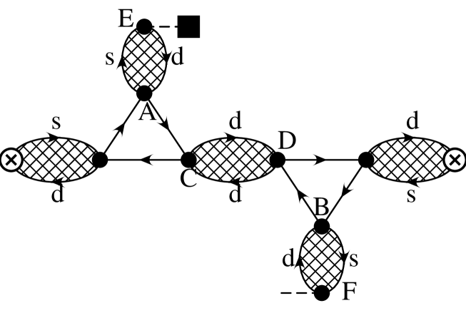
Figure 15: A leading $1/N_{c}$ contribution to the nonfactorizable part of $\Pi_{\Delta S=2}(q^{2})$ in the NJL model. The crosshatched areas are the full two-point functions as discussed in subsection 3.1. Point E and F are connected via $\Gamma_{\Delta S=2}$.

We now evaluate all contributions numerically to the two-point function of Eq. (329). The results for several input values are in table 2.

Table 2: Results for $B_{K}$ and $\hat{B}_{K}$ in the ENJL model.

$\mu$ (GeV)	$B_{K}^{\chi}(\mu)$	$\hat{B}{}_{K}^{\chi}$	$B_{K}^{m}(\mu)$	$B_{K}^{a}(\mu)$	$\hat{B}_{K}^{m}$	$B_{K}^{\rm eq}(\mu)$	$\hat{B}_{K}^{\rm eq}$
0.3	0.68	0.50	0.74	0.50	0.55	0.74	0.55
0.5	0.59	0.59	0.71	$-$0.44	0.71	0.72	0.72
0.7	0.53	0.58	0.69	$-$2	0.75	0.68	0.75
0.9	0.48	0.55	0.66	$-$3	0.76	0.65	0.75
1.1	0.45	0.54	0.64	$-$4	0.76	0.64	0.76

We have studied three cases, namely, the chiral case, $m_{d}=m_{s}=0$, the case with SU(3) symmetry breaking $m_{s}=83~{}{\rm MeV}\neq m_{d}=3~{}{\rm MeV}$ and the case with $m_{s}=m_{d}=43~{}{\rm MeV}$. The other parameters are $G_{S}=1.216$, $\Lambda_{\chi}=1.16~{}{\rm GeV}$ and $G_{V}=0$. The latter simplifies the calculation by about an order of magnitude. Preliminary results for the $G_{V}\neq 0$ case have the same qualitative conclusion[60] but typically somewhat lower values of $B_{K}$ and less good matching.

The procedure we have followed to analyze the numerical results is the following. We fit the ratio between the correction and the leading $1/N_{c}$ result for a fixed scale $\mu$ to $a/q^{2}+b+cq^{2}$ which always gives a very good fit ($a$, $b$ and $c$ are $\mu$ dependent). Once we have this fit we can extrapolate our $B_{K}$ form factor (remember that we have calculated it for Euclidean $q^{2}$) to the physical $B_{K}$, i.e. to $q^{2}=m_{K}^{2}\approx 0,0.13~{}{\rm GeV}^{2}$ (chiral,other cases).

Let us first treat the chiral or massless quarks case. Here a nontrivial check on the results is that the diagrams have a behaviour which sums to $1/q^{2}$, i.e. $a$ should be zero. The individual contributions do not have this behaviour. $b$ is the relevant contribution to $B_{K}$ since $m_{K}^{2}|_{\chi}=0$. The first three columns in table 2 are $\mu$, $B_{K}^{\chi}(\mu)$ and $\hat{B}_{K}^{\chi}=B_{K}(\mu)\alpha_{S}(\mu)^{a_{+}}$ with $a_{+}=-2/9$ and $\Lambda^{(3)}_{\overline{MS}}=250$ MeV. The hatted quantity is the scale independent quantity. Good matching is obtained if this value is stable within a range of $\mu$.

In the second case ($m_{s}\neq m_{d}$), because the chiral symmetry is broken, there is a possibility for contributions to $B_{K}(q^{2})$ that are not proportional to $q^{2}$, i.e. $a\neq 0$. In fact a CHPT calculation predicts precisely the presence of this type of terms[60]. For small values of $q^{2}$ the part due to $a$ dominates even though it is only a small correction when extrapolating to the physical $B_{K}^{m}$ at $q^{2}=m_{K}^{2}$. This can be found in column 4. The fifth column is the form factor $B_{K}^{a}$ for $q^{2}=-0.001$ GeV² where the correction due to the $a$ term is sizeable. Notice the difference between these two columns. This same feature should be visible in the lattice calculations as soon as they are done with different quark masses. The invariant $\hat{B}_{K}^{m}$ for this case is in column 6.

In the the last case, i.e. $m_{d}=m_{s}$, which is similar to the present lattice QCD calculations, the fit gives $a=0$ to a good precision and the value of $B_{K}^{\rm eq}$ extracted is rather independent of $q^{2}$. The invariant $\hat{B}_{K}^{\rm eq}$ in this case is in column 8.

In view of the results of [13, 10, 54] we expect to get a good prediction for the effects of non-zero and different current quark masses. We see those and find a significant change due to both:

$$\hat{B}_{K}^{m}(m_{K}^{2}\approx 0.13~{}{\rm GeV}^{2})\approx 1.35\,\hat{B}_{K}^{\chi}(m_{K}^{2}=0)$$ (333)

for scales $\mu\approx(0.7\sim 1.1)~{}{\rm GeV}$. For the extrapolation to the kaon pole the difference between the masses has a much smaller effect than the fact that they were non-zero. In order to compute $B_{K}$ in the general case a careful extrapolation to the poles was needed. The final correction to the $B_{K}$ parameter compared to its leading value of $3/4$ turns out to be rather small.

12 Conclusions

In this Physics Reports an overview of the results and the methods of references [13, 53, 61, 58, 54, 59] was given. There have also been several short versions given in talks and lectures[66, 65, 63, 64]. The main conclusion is that it is possible to use constituent chiral quark models and in particular the extended Nambu-Jona-Lasinio models to obtain results in the hadronic sector. The method underlying most of the results reviewed here allows for a clean separation of cut-off effects and consequences of the general structure of the model. This was especially clear in the case of the low-energy expansion, section 8 and the two-point functions, section 9. It also allowed for a discussion of the anomaly in the presence of extra pointlike quark interactions, section 7.

In the case of 3 and higher point functions the number of free functions in the general approach rapidly grows but still some general features are visible by the reduction to the basic one-loop functions.

The results also allowed the derivation of relations that are valid in a large class of Nambu-Jona-Lasinio like models. In particular the one with the inclusion of gluonic corrections. In fact the final results are rather insensitive to the inclusion of these extra effects precisely because the success of the ENJL model rests to a large extent on the relations we have derived here. These are also well satisfied by the hadronic experimental quantities we have tried to explain with this approach.

Especially the presence of several of the short-distance constraints from QCD in the ENJL model makes it a prime candidate for trying to estimate semi-analytically hadronic matrix elements. This has been done at present for the $\pi^{+}-\pi^{0}$ mass difference and the $B_{K}$ parameter. Both results have been reviewed here shortly.

In conclusion the simple extended nambu-Jona-Lasinio model provides us with a compact way to describe low-energy hadronic physics and understand a large body of experimental results. It also provides a framework to systematically explore effects due to explicit chiral symmetry breaking beyond chiral perturbation theory as shown here in the discussion about the $B_{K}$ parameter.

Appendix A Derivation of the Ward identities

In this appendix we generalize the proof in the appendix of ref. [53] to the case with nonzero current quark masses. There a proof was given of all relevant identities in terms of the heat kernel expansion (for an excellent recent review and definitions see ref. [45]) and some of them in terms of the Ward identities as well. Here those which can be derived directly from the Ward identities can also be derived from the heat kernel expansion but since they involve different masses they require a resummation of different terms. For these the direct derivation of the Ward identities is actually simpler. Only for the additional relations will we give the heat kernel derivation.

At the one-loop level we use as Lagrangian the one in eq. (13) (with the same definitions as there)

$${}{\cal L}_{\rm ENJL}=\overline{q}{\cal D}{q}$$ (A.1)

where $\cal D$ contains the couplings to the external fields $l_{\mu},r_{\mu},s$ and $p$ as well as the effects of the four-quark terms in ${\cal L}^{\rm S,P}_{\rm NJL}$ and ${\cal L}^{\rm V,A}_{\rm NJL}$ on the quark currents at the one-loop level. In particular it contains the constituent quark masses, $M_{i}$. However, we shall keep the notation $l_{\mu},r_{\mu},s$ and $p$ to denote the quark current sources in the presence of these four-quark NJL operators. The one-loop current identities derived from this Lagrangian are

$${}\partial^{\mu}V^{ij}_{\mu} = -i\left(M_{i}-M_{j}\right)S^{ij}$$

$$\partial^{\mu}A^{ij}_{\mu} = \left(M_{i}+M_{j}\right)P^{ij}\ .$$ (A.2)

When the whole series of constituent quark bubbles are summed these identities are satisfied changing constituent quark masses by current quark masses. In addition we use the equal time commutation relations for fermions

$${}\left\{q^{i{\dagger}}_{\alpha}(x),q^{j}_{\beta}(y)\right\}_{x^{0}=y^{0}}=i\delta_{\alpha\beta}\delta_{ij}\delta^{3}({\bf x}-{\bf y})\ .$$ (A.3)

Here $\alpha$ and $\beta$ are Dirac indices and $\bf x$ means the spatial components of $x$. Multiplying the two-point functions with $iq_{\mu}$ is equivalent to taking a derivative of the exponential under the integrals in eqs. (216) to (219). By partial integration we then get several terms, those due to the time ordering which leads to equal time commutators and those where the derivative hits one of the currents. The first type are evaluated using eq. (A.3) and the second type are related to other two-point functions using eq. (A). This then leads to the expressions (237) to (238).

The derivation of the other two identities is slightly more complicated. The effective action of the Lagrangian in eq. (A.1) can be obtained in Euclidean space as a heat kernel expansion (see ref. [45]). The coefficients of this expansion are the so-called Seeley-DeWitt coefficients, they are constructed out of the two quantities $E$ and $R_{\mu\nu}$. These are defined as

$${}{\cal D}^{\dagger}{\cal D} \equiv -\nabla_{\mu}\nabla^{\mu}+E+\overline{M}^{2}\ ,$$

$$R_{\mu\nu} \equiv \left[\nabla_{\mu},\nabla_{\nu}\right]\ ,$$

$$\nabla_{\mu}\# \equiv \partial_{\mu}\#-i[v_{\mu},\#]-i[a_{\mu}\gamma_{5},\#]\,.$$ (A.4)

If in eq. (A.1) the Dirac operator $\cal D$ contains couplings to gluons these should not be taken into account in eq. (A). The relevant heat kernel expansion in that case will have different coefficients depending on vacuum expectation values of gluonic operators, but will still be constructed out of the quantities in eq. (A) (depending now also on the gluon field). The quantity $\overline{M}$ is the mass that is used in the heat kernel expansion. The operator $\cal D$ is

$$i\gamma^{\mu}(\partial_{\mu}-iv_{\mu}-ia_{\mu}\gamma_{5})-{\cal M}-s+ip\gamma_{5}\ .$$ (A.5)

Here ${\cal M}={\rm diag}(m_{u},m_{d},m_{s})$ is the current quark mass matrix and we allow for spontaneous chiral symmetry breaking solution $\langle 0|s(x)|0\rangle\neq 0$. For the terms relevant to two-point functions we have

$${}R_{\mu\nu} = -i(v_{\mu\nu}+a_{\mu\nu}\gamma_{5})\,,$$

$${\rm and}\hskip 56.9055pt$$

$$E = -\frac{i}{2}\sigma^{\mu\nu}R_{\mu\nu}+i\gamma^{\mu}{\rm d}_{\mu}\left(M+s+ip\gamma_{5}\right)$$

$$- \gamma^{\mu}\left\{a_{\mu}\gamma_{5},M+s-ip\gamma_{5}\right\}+\left\{M,s\right\}-i\left[M,p\right]\gamma_{5}+s^{2}+p^{2}$$

$$+ M^{2}-\overline{M}^{2}\ ,$$

$${\rm with}$$

$$v^{\mu\nu} \equiv \partial^{\mu}v^{\nu}-\partial^{\nu}v^{\mu}-i[v^{\mu},v^{\nu}]\,,$$

$$a^{\mu\nu} \equiv \partial^{\mu}a^{\nu}-\partial^{\nu}a^{\mu}-i[a^{\mu},a^{\nu}]\,,$$

$${\rm d}^{\mu}\# \equiv \partial^{\mu}\#-i[v^{\mu},\#]\,.$$ (A.6)

The main difference with ref. [53] is the occurrence of the last line in the expression for $E$ in (A). We shall call this last line $E_{0}$. In this equation, $M\equiv{\rm diag}(M_{u},M_{d},M_{s})$, the diagonal matrix of the constituent quark masses defined in eq. (20). Notice that the scalar field here has been shifted and we have now $\langle 0|s(x)|0\rangle=0$ (though we use the same notation for it). When $G_{S}\to 0$ in eq. (20) then ${\overline{M}}\to 0$ and $M\to{\cal M}$. Let us now systematically go through all possible types of terms in the expansion. We shall not discuss the mixed two-point functions here since we only want to prove eqs. (241)-(242).

In the heat kernel expansion, those terms containing two factors $R_{\mu\nu}$ only contribute to the transverse parts, $\overline{\Pi}^{(1)}_{V,A}$ and in the same way. Their contributions hence obviously satisfy eqs. (241)-(242). Similarly, one factor $R_{\mu\nu}$ requires the presence of two covariant derivatives $\nabla_{\mu}$. By commuting derivatives (the extra terms only contribute to three and higher point functions) and partial integration these can be brought next to each other so they convert into a second factor $R_{\mu\nu}$. This brings us back to the previous case. Intervening $E$’s can only contribute via $E_{0}$ but these do not spoil the above argument. The first term in $E$, namely $\sigma_{\mu\nu}R^{\mu\nu}$, requires a 2nd $\sigma_{\mu\nu}R^{\mu\nu}$ because otherwise the trace over Dirac indices vanishes. These also behave like terms with two factors $R^{\mu\nu}$. Therefore, in the remainder we are only concerned with $E$ without this first term.

$E$ can also directly contribute to the scalar and pseudoscalar two-point function in the same way via $s^{2}+p^{2}$. Extra factors $E$ become again $E_{0}$ and extra derivatives also respect the relation (242). The most complicated case is where both fields come from a different $E$. This contributes in the form $E_{0}^{n}EE_{0}^{m}\partial^{2i}E$. These contribute to all form factors in the form $M_{i}^{n}M_{j}^{m}q^{2i}$ times the coefficients listed in Table 3.

Function	Contribution
$\overline{\Pi}_{S}$	$-q^{2}+(M_{i}+M_{j})^{2}$
$\overline{\Pi}_{P}$	$-q^{2}+(M_{i}-M_{j})^{2}$
$\overline{\Pi}^{(0)}_{A}$	$(M_{i}+M_{j})^{2}/q^{2}$
$\overline{\Pi}^{(1)}_{A}$	$-(M_{i}+M_{j})^{2}/q^{2}$
$\overline{\Pi}^{(0)}_{V}$	$(M_{i}-M_{j})^{2}/q^{2}$
$\overline{\Pi}^{(1)}_{V}$	$-(M_{i}-M_{j})^{2}/q^{2}$

Table 3: The contribution of terms of the type $E^{m+n+2}$ to the two-point functions.

These coefficients obviously satisfy the relations (241)-(242). The last type of terms is where the external fields come out of a derivative. We do not consider the mixed case here, so both the fields have to come out of a derivative due to the $\gamma_{\mu}$ that is necessarily present in the $E$ that would be a candidate for the external field. So there are those where the external fields are contained in two factors $\nabla_{\mu}$. If the indices of these are different, then there need to be at least two extra derivatives present that will produce a $q_{\mu}q_{\nu}$. This contributes equally to $\overline{\Pi}^{(0)}_{V}$ and $\overline{\Pi}^{(0)}_{A}$. If the indices are equal, it will contribute proportional to $g_{\mu\nu}$ and thus to the vector and axial-vector equally with $\overline{\Pi}^{(0+1)}_{V,A}=0$. This completes the proof of the identities (241)-(242).

Now it remains to prove that these contributions will never produce a pole in $\overline{\Pi}^{(0+1)}$ at $q^{2}=0$. Terms that contain two factors $R_{\mu\nu}$ contain two factors of momenta and hence do not. Terms with one factor $R_{\mu\nu}$ can be brought in the form with two so do not produce a pole either. From Table 3 there is no contribution from that type of terms to $\overline{\Pi}^{(0+1)}_{V,A}$. Then those with external fields from $\nabla_{\mu}$ with different derivatives necessarily contain extra factors $q_{\mu}q_{\nu}$ so do not contribute to a possible pole at $q^{2}=0$ and the last type of terms does not contribute to $\overline{\Pi}^{(0+1)}_{V,A}$ as shown above. This completes the proof.

Appendix B Explicit expressions for the barred two-point functions

Here we shall give the one-constituent-quark-loop expression for the two-point functions defined in eqs. (216)-(221) in the presence of current quark masses. These two-point functions are denoted in the text as the $\overline{\Pi}$ ones. They fulfil the same Ward identities as the full-ones in eqs. (237)-(240) changing the current quark masses there by the constituent quark ones. In addition, they also satisfy the Ward identities in eqs. (241)-(242). Using these identities one can see that there are only two independent functions out of $\overline{\Pi}^{(1)}_{V}$, $\overline{\Pi}^{(0)}_{V}$, $\overline{\Pi}^{(1)}_{A}$, $\overline{\Pi}^{(0)}_{A}$, $\overline{\Pi}_{S}^{M}$ $\overline{\Pi}_{P}^{M}$, $\overline{\Pi}_{S}$ and $\overline{\Pi}_{P}$. We shall take $\overline{\Pi}_{P}^{M}$ and $\overline{\Pi}^{(1)}_{V}+\overline{\Pi}^{(0)}_{V}$ as these functions. The explicit expressions are

$${}\left(\overline{\Pi}^{(1)}_{V}+\overline{\Pi}^{(0)}_{V}\right)(Q^{2})_{ij} = \frac{\displaystyle N_{c}}{\displaystyle 16\pi^{2}}\,8\,{\displaystyle\int^{1}_{0}}{\rm d}x\,x(1-x)\Gamma(0,x_{ij})\,,$$ (B.1)

$${}{\overline{\Pi}}_{P}^{M}(Q^{2})_{ij} = \frac{\displaystyle N_{c}}{\displaystyle 16\pi^{2}}\,4{\displaystyle\int^{1}_{0}}{\rm d}x(M_{i}x+M_{j}(1-x))\Gamma(0,x_{ij})\,,$$ (B.2)

where

$$x_{ij} \equiv \frac{\displaystyle M_{i}^{2}x+M_{j}^{2}(1-x)+Q^{2}x(1-x)}{\displaystyle\Lambda_{\chi}^{2}}\,.$$ (B.3)

One can obtain all the others one-loop two-point functions in function of these two by using the Ward identities mentioned above. For instance, for the $\overline{\Pi}^{(0)}_{V}$ one gets

$$\begin{array}[]{l}\displaystyle{}{\overline{\Pi}}^{(0)}_{V}(Q^{2})_{ij}=-\frac{\displaystyle\left(M_{i}-M_{j}\right)^{2}}{\displaystyle M_{i}+M_{j}}\,\frac{\displaystyle\overline{\Pi}^{M}_{P}(Q^{2})_{ij}}{\displaystyle Q^{2}(Q^{2}+(M_{i}-M_{j})^{2})}\\ \hskip 14.22636pt\times\left\{\left(M_{i}+M_{j}\right)^{2}+g_{A}(Q^{2})_{ij}m_{ij}^{2}(Q^{2})\left(1-\left(\frac{\displaystyle m_{i}-m_{j}}{\displaystyle m_{i}+m_{j}}\right)\left(\frac{\displaystyle M_{i}+M_{j}}{\displaystyle M_{i}-M_{j}}\right)\right)+Q^{2}\right\}\,.\\ \end{array}$$

Appendix C Explicit expression for the one-loop form factor $\overline{\Pi}^{+}_{\mu}(p_{1},p_{2})$

Here we shall give the one-constituent-quark-loop expression for the three-point function $\overline{\Pi}^{+}_{\mu}(p_{1},p_{2})$ defined in eq. (288). We shall give it for $M_{i}=M_{k}=M_{m}$. The explicit expression is (remember that we have $j=m$),

$${}\overline{\Pi}^{+\mu}(p_{1},p_{2}) =$$

$$- \frac{\displaystyle 1}{\displaystyle 2M_{i}}\Bigg{\{}\overline{\Pi}_{P}^{M}(-p_{1}^{2})_{ii}\,$$

$$+ \frac{\displaystyle p_{1}\cdot p_{2}}{\displaystyle p_{1}^{2}p_{2}^{2}-(p_{1}\cdot p_{2})^{2}}\,\left[p_{2}^{2}\left(\overline{\Pi}^{M}_{P}(-p_{2}^{2})_{ii}-\overline{\Pi}_{P}^{M}(-q^{2})_{ii}\right)\right.$$

$$+ \left.(p_{1}\cdot p_{2})\left(\overline{\Pi}_{P}^{M}(-p_{1}^{2})_{ii}-\overline{\Pi}_{P}^{M}(-q^{2})_{ii}\right)\right]$$

$$+ \frac{\displaystyle 2}{\displaystyle M_{i}}I_{3}(p_{1}^{2},p_{2}^{2},q^{2})p_{2}^{2}\left[1+(p_{1}\cdot p_{2})\frac{\displaystyle p_{1}^{2}+(p_{1}\cdot p_{2})}{\displaystyle p_{1}^{2}p_{2}^{2}-(p_{1}\cdot p_{2})^{2}}\right]\Bigg{\}}p_{1}^{\mu}$$

$$+ (p_{1}\leftrightarrow-p_{2})\,.$$

Where the two-point function $\overline{\Pi}^{M}_{P}(-p^{2})$ was given in appendix B and the function $I_{3}(p_{1}^{2},p_{2}^{2},q^{2})$ is

$$I_{3}(p_{1}^{2},p_{2}^{2},q^{2}) = \frac{\displaystyle N_{c}}{\displaystyle 16\pi^{2}}2M_{i}^{2}{\displaystyle\int^{1}_{0}}{\rm d}xx{\displaystyle\int^{1}_{0}}{\rm d}y\frac{\displaystyle\Gamma(1,M^{2}(x,y)/\Lambda_{\chi}^{2})}{\displaystyle M^{2}(x,y)}\,$$ (C.2)

with

$$M^{2}(x,y) \equiv$$

$$M_{i}^{2}-p_{1}^{2}(1-x)-p_{2}^{2}x(1-y)+(p_{1}(1-x)-p_{2}x(1-y))^{2}\,.$$

References

• [1] H. Fritzsch, M. Gell-Mann and H. Leutwyler, Phys. Lett. 47B (1974) 365; see e.g. P. Pascual and R. Tarrach, QCD: Renormalization for the practitioner, Lecture Notes in Physics, Springer Verlag, Vol. 194, Berlin, Germany, 1984.
• [2] S. Sharpe, Phenomenology from the lattice, lectures at TASI 94, UW/PT 94-15.
• [3] The DA$\Phi$NE Physics Handbook, eds. L. Maiani, G. Pancheri and N. Paver, INFN, Frascati 1992. A new edition is scheduled to appear in 1995.
• [4] See e.g. : L. Reinders, H. Rubinstein and S. Yazaki, Phys. Rep. 127 (1985) 1; S. Narison, QCD Spectral Sum Rules, World Scientific, Singapore, 1989.
• [5] J.Β Donoghue, E.Β Golowich and B.Β Holstein, Dynamics of the Standard Model, Cambridge University Press, Cambridge, 1992.
• [6] A. Manohar and H. Georgi, Nucl. Phys. B234 (1984) 189.
• [7] J. Bijnens and E. de Rafael, Phys. Lett. B273 (1991) 483.
• [8] D. Espriu, E. de Rafael and J. Taron, Nucl. Phys. B345 (1990) 22.
• [9] Y. Nambu and G. Jona-Lasinio, Phys. Rev. 122 (1961) 345.
• [10] T. Hatsuda and T. Kunihiro, Phys. Rep. 247 (1994) 221.
• [11] R. Cahill, Nucl. Phys. A543 (1992) 63c.
• [12] G. ’t Hooft, Nucl. Phys. B72 (1974) 461, B75 (1974) 461; E.Β Witten, Nucl. Phys. B160 (179) 57.
• [13] J. Bijnens, Ch. Bruno and E. de Rafael, Nucl. Phys. B390 (1993) 501.
• [14] H. Kleinert, Phys. Lett. 59B (1975) 163; 62B (1976) 429.
• [15] For a review of this work see M.K. Volkov, Part. and Nuclei, 24 (1993) 81.
• [16] A. Dhar and S. Wadia, Phys. Rev. Lett. 52 (1984) 959.; A. Dhar, R. Shankar and S. Wadia, Phys. Rev. D31 (1985) 3256.; S.R. Wadia, Prog. Theor. Phys. Suppl. 86 (1986) 26.
• [17] D. Ebert and M. Volkov, Z. Phys. C16 (1983) 205.
• [18] N. Karchev and A. Slavnov, Acta Physica Austriaca Suppl. XXV (1983) 357; Theor. Math. Phys. 65 (1986) 1099.
• [19] M. Volkov, Annal. Phys. 157 (1984) 282.
• [20] A. Dhar and S. Wadia, Phys. Rev. Lett. 52 (1984) 959.
• [21] D. Dyakonov and V. Petrov, Nucl. Phys. B245 (1984) 259.
• [22] D. Dyakonov and V. Petrov, Sov. Phys. JETP 62 (1985) 204, 431.
• [23] D. Ebert, Z. Phys. C28 (1985) 483.
• [24] R. Cahill and C. Roberts, Phys. Rev. D32 (1985) 2418.
• [25] A.A. Andrianov and Y. Novozhilov, Phys. Lett. B153 (1985) 422.
• [26] D. McKay and H. Munczek, Phys. Rev. D32 (1985) 266.
• [27] P. Simic, Phys. Rev. Lett. 55 (1985) 40.
• [28] P. Simic, Phys. Rev. D34 (1986) 1903.
• [29] A.A. Andrianov, Phys. Lett. B157 (1985) 425.
• [30] A.A. Andrianov, V.A. Andrianov, V.Yu. Novozhilov and Yu.V. Novozhilov, Lett. Math. Phys. 11 (1986) 217.
• [31] D. Ebert and H. Reinhardt, Phys. Lett. B173 (1986) 453.
• [32] D. Ebert and H. Reinhardt, Nucl. Phys. B271 (1986) 188.
• [33] A.A. Belkov, D. Ebert and V.N. Pervushin, Phys. Lett. B193 (1987) 315.
• [34] D. Dyakonov and V. Petrov, Nucl. Phys. B272 (1986) 457.
• [35] R.D. Ball, in Proc. Workshop on Skyrmions and Anomalies, Mogillany, Poland, 1987 (World Scientific, Singapore, 1988).
• [36] T.H. Hansson, M. Prakash and I. Zahed, Nucl. Phys. B335 (1990) 67.
• [37] E. Ruiz Arriola, Phys. Lett. B253 (1991) 430.
• [38] W. Weise, Hadrons in the NJL model, (Lectures given at Center for Theoretical Physics, Seoul National Univ., Seoul, Korea; September 1992) Regensburg preprint TPR-93-2.
• [39] S. Klimt et al., Nucl. Phys. A516 (1990) 429.
• [40] M. Lutz and W. Weise, Nucl. Phys. A518 (1990) 156.
• [41] D. Ebert and M. Volkov, Phys. Lett. B272 (1991) 86.
• [42] A.A. Khan et al., Spectroscopy and Renormalization groupl flow in the NJL model, FUB-HEP-93-14, hep-lat/9401012; K. Bitar and P. Vranas, Phys. Lett. B327 (1994) 101, Phys. Rev. D50 (1994) 3406.
• [43] J. Wess and B. Zumino, Phys. Lett. 37B (1971) 95;
E. Witten, Nucl. Phys. B223 (1983) 422.
• [44] A. Manohar and G. Moore, Nucl. Phys. B243 (1984) 55, there were several more around the same time, see the references in [45].
• [45] R.D. Ball, Phys. Rep. 182 (1989) 1.
• [46] R.I. Nepomechie, Ann. Phys. (NY) 158 (1984) 67.
• [47] J. Balog, Phys. Lett. 149 (1984) 197.
• [48] A.A. Andrianov and L. Bonora, Nucl. Phys. B233 (1984) 232.
• [49] J. Zuk, Z. Phys. C29 (1985) 303.
• [50] A. Pich and E. de Rafael, Nucl. Phys. B358 (1991) 311.
• [51] E. de Rafael, in Proc. LP-HEP 91 Conference, Geneva, 1991.
• [52] J. Bijnens, Nucl. Phys. B367 (1991) 709.
• [53] J. Bijnens, E. de Rafael and H. Zheng, Z. Phys. C62 (1994) 437.
• [54] J. Bijnens and J. Prades, Z. Phys. C64 (1994) 475.
• [55] U.Β Vogl et al., Nucl. Phys. A516 (1990) 156.
• [56] L.S. Celenza et al., Axial-vector isovector hadronic current correlator in a NJL model, Brooklyn preprint, BCCNT-93-093-236 and references therein.
• [57] V.Β Bernard et al., Phys. Lett. B324 (1994) 201.
• [58] J. Bijnens and J. Prades, Phys. Lett. B320 (1994) 130.
• [59] J.Β Bijnens and J.Β Prades,Phys. Lett. B342 (1995) 331.
• [60] J. Bijnens and J. Prades, The $B_{K}$-Parameter in the $1/N_{c}$ Expansion, NORDITA-95/11 N,P.
• [61] J. Prades, Z. Phys. C63 (1994) 491.
• [62] E. de Rafael, Phys. Lett. B322 (1994) 239.
• [63] E. de Rafael, presented at the International Conference on Highh-Energy Physics, Dallas, texas, August 1992.
• [64] E. de Rafael, presented at Hadron93, Como, Italy, June 1993, CPT-93/P.2967, hep-ph 9312327.
• [65] J. Bijnens, Introduction to the Extended Nambu-Jona-Lasinio model, to appear in the second edition of [3], NORDITA 94/27 N,P, hep-ph 9406425.
• [66] J. Bijnens, Effective Lagrangians for light quarks, 7th Adriatic meeting on particle physics, NORDITA 94/65 N,P, hep-ph/9411420, to be published in the proceedings.
• [67] J. Bijnens and J. Prades, 2 and 3-point functions in the ENJL model, presented at QCD94, Montpellier, July 1994, NORDITA 94/43 N,P, hep-ph/9409231.
• [68] J. Gasser and H. leutwyler, Ann. Phys. 158 (1984) 142.
• [69] J. Gasser and H. Leutwyler, Nucl. Phys. B250 (1985) 465.
• [70] K. Yamawaki and V.I. Zakharov, Extended Nambu-Jona-Lasinio model vs QCD sum rules, UM-TH94-19, hep-ph/9406373.
• [71] See e.g., Yu. Kalinowski et al., Sov. J. Nuc. Phys. 49 (1989) 1059, V.N. Pervushin, Nucl. Phys. B(proc. Suppl.)15 (1990) 197.
• [72] A.A. Andrianov et al., Phys. Lett. B328 (1994) 401.
• [73] E. Pallante and R. Petronzio, The Quark-Resonance Model, ROM2F-94-32, hep-ph/9408232.
• [74] E. Witten, Nucl. Phys. B160 (1979) 57, B156 (1979) 269; G. Veneziano, Nucl. Phys. B159 (1979) 269; P. di Vecchia and G. Veneziano, Nucl. Phys. B171 (1980) 253; E. Witten, Ann. of Phys. 128 (1980) 363; C. Rosenzweig, J. Schechter and C.G. Trahern, Phys. Rev. D21 (1980) 3388.
• [75] S. Coleman and E. Witten, Phys. Rev. Lett. 45 (1980) 100.
• [76] See, e.g., S. Gottlieb et al., Phys. Rev. D35 (1987) 3972.
• [77] J. Bijnens, J. Prades and E. deΒ Rafael, Light Quark masses in QCD, NORDITA 94/62 N,P, CPT-PE3079, hep-ph/9411285, to be published in Phys. Lett. B.
• [78] H. Leutwyler, Nucl. Phys. B (Proc. Suppl.) 7A (1989) 42.
• [79] J.Gasser, in Proc. LP-HEP 91 Conference, Geneva, 1991.
• [80] A. Pich, in Proc. LP-HEP 91 Conference, Geneva, 1991.
• [81] G. Ecker, Chiral Perturbation Theory, UWThPh-1994-49, hep-ph/9501357.
• [82] J. Bijnens, Nucl. Phys. B337 (1990) 635;
J. Donoghue, J. Gasser, B. Holstein and C. Riggenbach, Phys. Rev. D43 (1991) 127;
J. Bijnens, G. Colangelo and J. Gasser, Nucl. Phys. B427 (1994) 427.
• [83] S. Coleman, J. Wess and B. Zumino, Phys. Rev. 177 (1969) 2237;
C. Callan and S. Coleman, Phys. Rev. 177 (1969) 2247.
• [84] G. Ecker, J. Gasser, A. Pich and E. de Rafael, Nucl. Phys. B321 (1989) 311.
• [85] G. Ecker, J. Gasser, H. Leutwyler, A. Pich and E. de Rafael, Phys. Lett. B223 (1989) 425.
• [86] U.-G. Meissner, Phys. Rep. 161 (1988) 213 and references therein.
• [87] M. Bando, T. Kugo and K. Yamawaki, Phys. Rep. 164 (1988) 217 and references therein.
• [88] S. Weinberg, Phys. Rev. 166 (1968) 1568, Sect. VII.
• [89] E. Pallante and R. Petronzio, Nucl. Phys. B396 (1993) 205.
• [90] S. Peris and E. de Rafael, Phys. Lett. B309 (1993) 389; W. Broniowski et al., Phys. Rev. Lett. 71 (1993) 1787.
• [91] E. Ruiz-Arriola and L.L. Salcedo, Phys. Lett. B316 (1993) 148.
• [92] Y. Brihaye, N.K. Pak and P. Rossi, Nucl. Phys. B254 (1985) 71.
• [93] W.A. Bardeen, Phys. Rev. 184 (1969) 1848.
• [94] K. Fujikawa, Phys. Rev. Lett. 42 (1979) 1195; Phys. Rev. D21 (1980) 2848.
• [95] W.A. Bardeen and B. Zumino, Nucl. Phys. B244 (1984) 421.
• [96] H. Leutwyler, Phys. Lett. B152 (1985) 78.
• [97] T. Fujiwara et al., Prog. Theor. Phys. 73 (1985) 926.
• [98] J. Bijnens, Int. J. Mod. Phys. A8 (1993) 3045.
• [99] M. Wakamatsu, Ann. of Phys. 193 (1989) 287.
• [100] S. Weinberg, Phys. Rev. Lett. 18 (1967) 507.
• [101] M. Praczalowicz and G. Valencia, Nucl. Phys. B341 (1990) 22.
• [102] M. Froissart, Phys. Rev. 123 (1961) 1053.
• [103] H. Leutwyler and M.A. Shifman, Nucl. Phys. B343 (1990) 369.
• [104] M.A. Shifman, A.I. Vainshtein and V.I. Zakharov, Nucl. Phys. 147 (1979) 385, 448.
• [105] H. Fearing and S. Scherer, Extension of the CHPT meson lagrangian to order $p^{6}$, TRIUMF TRI-PP-94-68, hep-ph/9408346.
• [106] E.G. Floratos, S. Narison and E. de Rafael, Nucl. Phys. B155 (1979) 115.
• [107] P. Pascual and E. de Rafael, Z. Phys. C12 (1982) 127; S. Narison, Z. Phys. C14 (1982) 263.
• [108] M. Gell-Mann, R. Oakes and B. Renner, Phys. Rev. 175 (1968) 2195.
• [109] Ll. Ametller et al., Nucl. Phys. B228 (1983) 301; A. Pich and J. BernabΓ©u, Z. Phys. C22 (1984) 197
• [110] S.L. Adler and W.A. Bardeen, Phys. Rev. 182 (1969) 1517
• [111] K. Kawarabayashi and M. Suzuki, Phys. Rev. Lett.16 (1966) 255; Riazuddin and Fayyazuddin, Phys. Rev. 147 (1966) 1071.
• [112] CELLO Colaboration, H.-J. Behrend et al., Z. Phys. C49 (1991) 401.
• [113] J. Bijnens, A. Bramon and F. Cornet, Z. Phys. C46 (1990) 599; J. Bijnens, Int. J. Mod. Phys. A8 (1993) 3045.
• [114] J.-M. GΓ©rard, Acta Physica Polonica B21 (1990) 257.
• [115] W.A.Β Bardeen et al., Phys. Rev. Lett. 62 (1989) 1343.
• [116] T. Das et al., Phys. Rev. Lett. 18 (1967) 759.
• [117] J.Β Donoghue and E.Β Golowich, Phys. Rev. D49 (1994) 1513.
• [118] W.A. Bardeen, A. Buras and J.-M. GΓ©rard, Phys. Lett. B211 (1988) 371.
• [119] Proceedings of the Ringberg Workshop on Hadronic Matrix Elements and Weak Decays, Ringberg, Germany, april 1988, eds. A.J. Buras, J.-M. GΓ©rard and W. Huber, Nucl. Phys. B(Proc. Suppl.) 7A (1989)
• [120] S.R. Sharpe, Nucl. Phys. B(Proc. Suppl.) 34 (1994) 403;
N. Ishizuka et al., Phys. Rev. Lett. 71 (1993) 24.
• [121] A. Pich and E. de Rafael, Phys. Lett. B163 (1985) 198; K.G. Chetyrkin et al., Phys. Lett. B174 (1986) 104; R. Decker, Nucl. Phys. B277 (1986) 661, in [119]; N. BiliΔ‡ et al., Z. Phys. C39 (1988) 351; J. Prades et al., Z. Phys. C51 (1991) 287; L.J. Reinders and S. Yazaki, Nucl. Phys. B288 (1987) 789.