CERN-TH/95-26 UM-TH-95-3 hep-ph/9502300 February 1995

Resummation of $(\beta_{0}\alpha_{s})^{n}$ Corrections in QCD: Techniques and Applications to the $\tau$ Hadronic Width and the Heavy Quark Pole Mass

Patricia Ball¹, M. Beneke² and V.M. Braun³

¹CERN, Theory Division, CH–1211 Genève 23, Switzerland
²Randall Laboratory of Physics, University of Michigan, Ann Arbor, Michigan 48109, USA
³DESY, Notkestraße 85, D–22603 Hamburg, Germany

Abstract:
We propose to resum exactly any number of one-loop vacuum polarization insertions into the scale of the coupling of lowest order radiative corrections. This makes maximal use of the information contained in one-loop perturbative corrections combined with the one-loop running of the effective coupling and provides a natural extension of the familiar BLM scale-fixing prescription to all orders in the perturbation theory. It is suggested that the remaining radiative corrections should be reduced after resummation. In this paper we implement this resummation by a dispersion technique and indicate a possible generalization to incorporate two-loop evolution. We investigate in some detail higher order perturbative corrections to the $\tau$ decay width and the pole mass of a heavy quark. We find that these corrections tend to reduce $\alpha_{s}(m_{\tau})$ determined from $\tau$ decays by approximately 10% and increase the difference between the bottom pole and $\overline{\rm MS}$-renormalized mass by 30%.

1 Introduction

During the past decade QCD has turned from qualitative descriptions to quantitative predictions for the strong interactions. The influx of more accurate experimental data represents a constant stimulus to improve theoretical predictions. While an understanding of confinement remains as evasive as ever, these predictions rely on the validity of nonperturbative factorization in processes governed by a large momentum scale. This allows to isolate the presently uncalculable infrared dynamics in a set of universal parameters or functions. One is then led to the conclusion that relations of physical quantities can be calculated in perturbation theory. For certain observables, such as those derived from totally inclusive processes with no hadrons in the initial state, one obtains parameter-free predictions (except for the strong coupling) to logarithmic accuracy in the hard scale.

Much effort has been invested in the computation of higher order QCD radiative corrections. For a few observables for which quark masses are unimportant, second order corrections in the strong coupling $\alpha_{s}$ are known. Third order expressions exist for hadroproduction in $e^{+}e^{-}$-annihilation and $\tau$-lepton decays and for the Gross-Llewellyn-Smith and Bjorken sum rule in deep inelastic scattering. On the other hand, observables involving quark masses, for example decay widths of hadrons containing a heavy quark, are known only to first order. In most cases, the extension of present results is not simply a question of algebraic complexity and algorithms for handling it. The existing calculations have exploited presently known techniques to the frontier beyond which new methods need to be designed, a task which might not be completed soon. In this situation it is interesting to explore possible sources of systematically large corrections in higher orders, which, once identified, might then be taken into account exactly to all orders. In doing so, one may hope to reduce the uncertainty due to ignorance of exact higher order coefficients.

Resummations of this type are familiar and necessary for many problems involving disparate mass scales. Large perturbative corrections in higher orders are associated with a logarithm of the ratio of these scales and can often be summed with renormalization group techniques, which allow to obtain the dominant power of that logarithm to all orders by one-loop calculations. Although in practice it is not always clear whether the logarithms dominate the constant pieces – in particular, since the coefficients of logarithms grow geometrically with order of $\alpha_{s}$, whereas the constants grow factorially –, such a resummation is controlled by an “external” parameter (the logarithm of two scales) that can be varied, at least in fictitious limits. For the problem at hand, we assume that such renormalization group improvement has already been done or consider observables that depend only on a single scale. We are thus interested in systematically large contributions to constant terms with no external scale at our disposal. 1

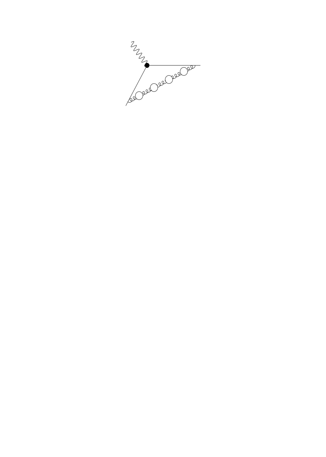
Figure 1: A typical diagram with multiple fermion loop insertions into the lowest order correction to a generic physical quantity.

The estimation of constant terms of yet uncalculated coefficients, which is closely related to the problem of scale- and scheme-setting for truncated perturbative expansions, is often thought to attempt the impossible. While indeed for any particular observable it is impossible to assess with rigour the quality of a certain scale-setting prescription, some prescriptions may be supported by general physical arguments and turn out to be closer to exact results a posteriori. The most distinguished prescription of this kind has been formulated by Brodsky, Lepage and Mackenzie [1]. Observing that in QED all scale-dependence of the coupling results from photon vacuum polarization, they suggested that the effect of fermion loop insertions into a photon line in higher orders be absorbed into the scale of the coupling of a given order and proposed to apply this criterion to QCD as well. In practical applications, this suggestion has mainly been realized in second order in $\alpha_{s}$. To this accuracy, only a single fermion loop insertion needs to be calculated and the relevant contribution can be traced by its dependence on the number of light fermions $N_{f}$. In general, at order $\alpha_{s}^{n+1}$, the effect of one-loop evolution of the coupling can still be obtained by the highest power of $N_{f}$ in the flavour-dependence of coefficients. The highest power of $N_{f}$ originates solely from diagrams with $n$ fermion loop insertions, such as in Fig. 1, which are much easier to calculate than flavour-independent terms. In QCD, the identification of contributions related to one-loop renormalization of the coupling implies that the coefficient of the highest power in $N_{f}$ should in fact not multiply $N_{f}$ to some power, but the combination $N_{f}-33/2$, as it appears in the Gell-Mann-Low function to leading order. Computing diagrams as in Fig. 1 and then replacing $N_{f}$ by $N_{f}-33/2$, one takes into account partial contributions from other diagrams, which are much harder to evaluate exactly (the precise identification of these contributions with particular diagrams is not straightforward and gauge-dependent). It turns out that in all cases where comparison with exact second order results is possible, this replacement approximates the exact coefficient amazingly well in the $\overline{\rm MS}$-scheme [2]. In what follows we shall refer as “Naive Nonabelianization” (NNA) [3] to the hypothesis that a substantial part of higher order radiative corrections can be accounted for by running of the coupling, in the sense of substitution of $N_{f}\rightarrow N_{f}-33/2$ in the term with the highest power of $N_{f}$. We should mention that BLM scale-setting and NNA are technically identical and the distinction is rather a matter of interpretation: The BLM scale-setting by its physical motivation does not necessarily claim that genuine higher order corrections missed by the above substitution should be small, whereas NNA assumes this stronger assertion.

This paper is concerned with an exposition of details of the recent proposal [4] of two of us to extend the BLM procedure to higher orders and, in particular, to sum all contributions associated with one-loop running of the coupling. We emphasize that this procedure has repeatedly been suggested in the past [1, 5], but has apparently not been pursued to the point of practical implementation. A summation similar to, but technically different from [4] was also presented in [6]. We believe that this resummation is useful, because the effect of evolution of the coupling is a systematic source of potentially large perturbative coefficients. In such a situation it is advantageous to incorporate this effect in theoretical predictions even if it transcends a fixed-order perturbative approximation.

To become definite, we use the following convention for the QCD $\beta$-function:

$$\mu^{2}\frac{d\alpha_{s}}{d\mu^{2}} = \beta(\alpha_{s})=\beta_{0}\alpha_{s}^{2}+\beta_{1}\alpha_{s}^{3}+\ldots\,;$$

$$\beta_{0} = -\frac{1}{4\pi}\left(11-\frac{2}{3}N_{f}\right)\,,\hskip 14.22636pt\beta_{1}=-\frac{1}{(4\pi)^{2}}\left(102-\frac{38}{3}N_{f}\right)\,.$$ (1.1)

For a generic physical observable $R$ (which for the sake of illustration we assume to depend only on a single, large scale $Q$), we may eliminate the $N_{f}$-dependence in radiative corrections in favour of the $\beta$-function coefficients $\beta_{0}$, $\beta_{1}$ etc. For now (and most parts of this paper) we restrict ourselves to one-loop running, induced by $\beta_{0}$. The (truncated) perturbative expansion of $R$ is written as

$$R-R_{tree} = \sum_{n=0}^{N}[r_{n0}+r_{n1}N_{f}+\ldots+r_{nn}N_{f}^{n}]\alpha_{s}(Q)^{n+1}$$ (1.2)

$$= r_{0}\alpha_{s}(Q)\sum_{n=0}^{N}\left[\delta_{n}+d_{n}(-\beta_{0})^{n}\right]\alpha_{s}(Q)^{n}\,,$$

where

$$d_{n}=(-6\pi)^{n}\frac{r_{nn}}{r_{0}}\,.$$ (1.3)

Let us stress again that $d_{n}$ is unambiguously determined by diagrams with $n$ insertions of fermion bubbles as in Fig. 1 and only $\delta_{n}$ requires a true $n+1$-loop calculation. The $\delta_{n}$ ($n\geq 2$) could be further separated into contributions from two-loop evolution and the effect of one-loop evolution on the genuine two-loop corrections (see [7] for $\delta_{2}$). We introduce

$$M_{N}(-\beta_{0}\alpha(Q))=1+\sum_{n=1}^{N}d_{n}(-\beta_{0}\alpha(Q))^{n}$$ (1.4)

as a measure of how much the lowest order correction is modified by summing $N$ one-loop vacuum polarization insertions. To make an explicit connection to BLM scale-setting, we define

$$\alpha_{s}(Q^{*}_{N})=\alpha_{s}(Q)\,M_{N}(-\beta_{0}\alpha_{s}(Q))\,$$ (1.5)

absorbing the effect of vacuum polarization in the scale $Q_{N}^{*}$ of the coupling. For $N=\infty$, $\alpha_{s}(Q^{*})$ ($Q^{*}\equiv Q^{*}_{\infty}$) is transparently interpreted as the running coupling averaged over the lowest order corrections. Isolating the integration over gluon virtuality in the lowest-order diagram, we may write

$$r_{0}\alpha_{s}(Q)=\alpha_{s}(Q)\int\mbox{d}^{4}k\,F(k,Q)\,\frac{1}{k^{2}}.$$ (1.6)

Then

$$r_{0}\alpha_{s}(Q^{*})=\frac{r_{0}\alpha_{s}(Q)}{1-\beta_{0}\alpha_{s}(Q)\ln({Q^{*}}^{2}/Q^{2})}=\int\mbox{d}^{4}k\,F(k,Q)\,\frac{\alpha_{s}\left(k\exp[C/2]\right)}{k^{2}},$$ (1.7)

where $C$ is a the scheme-dependent subtraction constant for the fermion loop. The difference between the leading-order BLM scale $Q_{1}^{*}$ and $Q^{*}$ is precisely the difference between averaging the running coupling itself, or the logarithm of its argument, over the lowest-order diagram. The values of $Q^{*}$ and $Q^{*}_{N}$ for $N>1$ depend on the value of $\alpha_{s}(Q)$. Such a dependence is intrinsic to any generalization of the BLM prescription beyond leading-order and has previously been noted in [8, 7]. As a result we may express any physical quantity as

$$R-R_{tree}=r_{0}\left(\alpha(Q)M_{\infty}(-\beta_{0}\alpha_{s}(Q))+\sum_{n=1}^{\infty}\delta_{n}\alpha_{s}(Q)^{n+1}\right)\,.$$ (1.8)

Separating radiative corrections in this way and summing a partial set of them into $M_{\infty}(-\beta_{0}\alpha_{s})$ can be motivated in different ways. First of all, as already mentioned, this procedure is supported empirically at the two-loop level. Provided the three-loop coefficient is sizeable, one might again expect that a significant portion of it can already be accounted for by $M_{2}(-\beta_{0}\alpha_{s})$ and, in higher orders, by $M_{N}(-\beta_{0}\alpha_{s})$.

It must be noted that such a statement depends on the choice of scheme and, since the $\delta_{n}$ depend on $N_{f}$ for $n>1$, also on $N_{f}$ for a given scheme. Although $Q^{*}$ is defined such that $\alpha_{s}(Q^{*})$ is scheme-independent if one consistently uses the one-loop $\beta$-function, an arbitrary $N_{f}$-independent finite renormalization can always ruin the supposed dominance of $\beta_{0}^{n}\alpha_{s}^{n+1}$-terms by implying a definition of the coupling that leads to anomalously large values of the remaining terms $\delta_{n}$. This remark applies of course to any partial resummation, whether it is based on a systematic (external) parameter or not as in the case at hand. In this respect a resummation utilizing one-loop running is similar to resummation of $\pi^{2}$’s that arise from analytic continuation from the space-like to the time-like region of, for instance, the Sudakov form factor [9] or the coupling as in $e^{+}e^{-}$-annihilation or $\tau$ decays [10], and, in fact, comprises the resummation for $\tau$ decays as a special case. Since empirically the $\beta_{0}$-term dominates second order radiative corrections for many observables in the $\overline{\rm MS}$ scheme, one would not expect the resummation of $\beta_{0}\alpha_{s}^{n+1}$-terms to be numerically useful in schemes that differ from $\overline{\rm MS}$ by a redefinition of the coupling that changes significantly the relative importance of flavour-dependent and flavour-independent terms.

The dominance of $\beta_{0}^{n}\alpha_{s}^{n+1}$-terms is lended further support from the behaviour of perturbative coefficients in large orders (renormalons). It is precisely the effect of vacuum polarization, which leads to the expectation that in sufficiently large orders, the coefficients should indeed have the form

$$r_{n}\sim K\,(a\beta_{0})^{n}n!n^{b}\,.$$ (1.9)

The series is thus divergent and, provided it is asymptotic at all, cannot approximate the true result to any desired accuracy, even if the exact coefficients could be computed to arbitrary order. The evaluation of diagrams as in Fig. 1 provides some insight into this ultimate limitation of perturbative QCD and into the approach to the asymptotic limit. In this paper, however, we are not so much interested in large orders and effects suppressed by powers of the hard scale $Q$. Summation of effects associated with one-loop running of the coupling should prove useful in intermediate orders (say, $n=2-6$), when perturbation theory is still reliable. It is amusing to speculate whether the empirical dominance of $\beta_{0}$ at the two-loop level indicates that one is already close to the asymptotic behaviour. The latter is derived from a saddle point expansion and the large contribution arises from internal momenta either much smaller or much larger than the external scale $Q$. Proximity to the asymptotic behaviour – if true – would indicate that the distribution of internal momenta is already well-approximated by a Gaussian even though the main contribution to the Feynman integral is not from small or large momenta.

The consideration of large orders provides also useful guidance to the limitations that arise from the restriction to one-loop evolution effects. As a matter of fact, diagrams associated with one-loop evolution do not provide the correct constants $b$ and $K$ in the large-$n$ behaviour. At large $n$, the effect of two-loop evolution on a single gluon line and one-loop evolution on two gluon lines becomes equally important and should eventually be taken into account. In practical applications, we will often find that the series has to be truncated due to its divergence at rather low $n$. Thus, many diagrams which are required to establish the formal large-$n$ behaviour never become relevant. Moreover, provided $\delta_{1}$ is already not large, one should also expect that vacuum polarization insertions into two gluon lines will remain comparatively small.

Let us repeat that the resummation of $\beta_{0}^{n}\alpha_{s}^{n+1}$-terms can only be judged a posteriori and can fail to provide a good estimate of higher order corrections for any particular quantity. Even in this case, we believe that this resummation is physically motivated and that it is appropriate to absorb this particular class of higher order corrections into the scale of the coupling in lowest order. Application of BLM scale-setting to leading order (absorbing the contribution from one fermion loop) yields $Q_{1}^{*}=Qe^{-d_{1}/2}$. Upon re-expansion of $\alpha_{s}(Q_{1}^{*})$ to one-loop accuracy for the $\beta$-function, this pretends a geometric growth $d_{n}^{\rm BLM}=d_{1}^{n}$ to be compared with the factorial growth of the exact coefficients. Resummation to all orders corrects for this discrepancy by adjusting $Q^{*}_{\infty}$ such that the expansion of $\alpha_{s}(Q^{*}_{\infty})$ gives the correct values of $d_{n}$. Thus to the accuracy of one-loop evolution the result of resummation is equivalently expressed as $\alpha_{s}(Q)M_{\infty}(-\beta_{0}\alpha_{s})$ and we often prefer this form of presentation. It is no longer equivalent to $\alpha(Q^{*}_{\infty})$, if one adopts two-loop accuracy for $\alpha_{s}$. Since for large $n$ the true $d_{n}$ will always outgrow $d_{1}^{n}$, one might conclude that the usual BLM scale-setting underestimates higher order radiative corrections. In practice, the effect is often just the opposite: The most important contributions come from intermediate $n$ and it turns out that in many cases $d_{1}$ is comparatively large ($Q_{1}^{*}$ is small), so that $d_{1}^{n}>d_{n}$ in this region. The usual BLM scale-setting therefore typically overestimates the size of radiative corrections associated with one-loop running.

The remainder of the paper is organized as follows: In Sect. 2 we develop in detail the technique to implement the resummation. We use a dispersion technique to reduce the problem to a one-dimensional integral over lowest order radiative corrections computed with finite gluon mass which is suitable to numerical evaluation. Thus compared to the complications of a complete higher order calculation, this resummation can be performed with little computational expense. Compared to a similar implementation of the standard BLM scale-setting [12], the computation of higher order coefficients $d_{n}$ comes with no additional expense at all. It is convenient to introduce the Borel transform as a generating function of higher order radiative corrections. The principal value definition of the Borel integral serves as a starting point for the summation of the series within a certain accuracy, indicated by the presence of infrared renormalons. We shall also see that this definition requires all kinematic invariants to be large compared to $\Lambda_{\rm QCD}$, reflecting the inapplicability of perturbation theory as a starting point for summation, if this requirement is not met. In this Section we also generalize the results of [4] to quantities with anomalous dimension and include quarks with finite masses in the loops.

In Sect. 3 we apply the resummation to the hadronic width of the $\tau$ lepton and find a 10% decrease of $\alpha_{s}(m_{\tau})$ due to four- and higher loop corrections. We discuss the possibility of $1/m_{\tau}^{2}$-corrections in the light of our resummation. In general we prefer to be agnostic about power corrections and stick to perturbation theory. An exception to this rule is that we do not want to introduce power corrections in conflict with the operator product expansion in euclidian space without good reasons (which we do not have). Under this assumption we show that principal value resummation does not introduce $1/m_{\tau}^{2}$-terms to the decay width, provided the coupling is chosen appropriately. Sect. 4 contains a detailed discussion of the resummation of $(-\beta_{0})^{n}\alpha_{s}^{n+1}$-terms for the pole mass of a heavy quark. We combine the resummation with the exact two-loop result to give an estimate of the difference between the pole mass and the $\overline{\rm MS}$-renormalized mass. We keep finite quark masses inside loops which allows to trace the origin of large coefficients to the relevant regions of internal momentum.

In Sect. 5 we formulate one possible extension of our resummation to incorporate partially the effect of two-loop running resulting in $\beta_{1}\beta_{0}^{n-2}$-corrections. This extension is again guided by the flavour-dependence of coefficients and can be considered as an extension of recent work by Brodsky and Lu [7]. The size of corrections is illustrated for the vector correlation function relevant to $\tau$ decays and for the pole mass of a heavy quark. Sect. 6 contains conclusions. Three Appendices deal with technical issues: In Appendix A we derive a simple expression for subtractions needed for logarithmically ultraviolet divergent quantities and collect the details of results presented in Sect. 2. Appendix B contains analytic formulae for the lowest order radiative corrections to $R_{e^{+}e^{-}}$ and hadronic $\tau$ decays with finite gluon mass. In Appendix C we list exact results for some abelian five-loop diagrams to the vector correlation function.

In a companion paper [13] we shall discuss the implications of resummation for heavy quark decays and the determination of $|V_{bc}|$.

2 Techniques

The aim of this Section is to develop a systematic approach to the calculation of diagrams with an arbitrary number of fermion loop insertions, such as in Fig. 1. We assume a generic physical (short-distance) quantity $R$ and a renormalization scheme that does not introduce an artificial $N_{f}$ dependence, such as $\overline{\rm MS}$. It is also assumed that lowest order radiative corrections to $R$ do not involve the gluon self-coupling. Subtracting the tree-level contribution, we are left with the (truncated) perturbative expansion

$$R-R_{tree}=\sum_{n=0}^{N}r_{n}\alpha_{s}^{n+1}\,.$$ (2.1)

The coefficients $r_{n}$ are polynomials in $N_{f}$ ,

$$r_{n}=r_{n0}+r_{n1}N_{f}+\ldots+r_{nn}N_{f}^{n},$$ (2.2)

and we will calculate the coefficients $r_{nn}$, which originate from $n$ fermion loop insertions into the lowest-order diagram. We then write

$$r_{n}=r_{0}\left[\delta_{n}+(-\beta_{0})^{n}d_{n}\right],$$ (2.3)

where $d_{n}=(-6\pi)^{n}r_{nn}/r_{0}$ absorbs the term with the largest power of $N_{f}$. The effect of one-loop evolution of the coupling on lowest order radiative corrections is then entirely contained in the $d_{n}$ and in the remainder of the paper we will consider the $\delta_{n}$ as corrections to the approximation of “Naive Nonabelianization”. As a measure of how much the lowest order radiative correction is modified by including $N$ vacuum polarization insertions, we define

$$M_{N}(-\beta_{0}\alpha_{s}) \equiv 1+\sum_{n=1}^{N}d_{n}(-\beta_{0}\alpha_{s})^{n}\,,$$

$$M_{\infty}(-\beta_{0}\alpha_{s}) \equiv M_{N\to\infty}(-\beta_{0}\alpha_{s})\,.$$ (2.4)

Taken literally, the limit $N\rightarrow\infty$ does not exist, because the series diverges. It will be interpreted in the sense of Eq. (2.8) below. For further use, we introduce the shorthand notation

$$a_{s}(\mu)=-\beta_{0}\alpha_{s}(\mu)\,,$$ (2.5)

where $\mu$ is the normalization scale, which often will be suppressed for brevity. In this Section we are concerned only with technical aspects of the calculation of $M_{N}(a_{s})$ and $M_{\infty}(a_{s})$.

2.1 Borel transform vs. finite gluon mass

A convenient way to deal with diagrams with multiple loop insertions is to calculate the Borel transform

$$B[R](u)\equiv\sum_{n}\frac{r_{n}}{n!}(-\beta_{0})^{-n}u^{n}\,,$$ (2.6)

which can be used as a generating function for the fixed-order coefficients [14]:

$$r_{n}=(-\beta_{0})^{n}\frac{d^{n}}{du^{n}}B[R](u)_{|_{u=0}}\,.$$ (2.7)

Another advantage of presenting the results in form of the Borel transform is that the result for the sum of all diagrams can easily be recovered by the integral representation

$$r_{0}M_{\infty}(a_{s})=\frac{1}{a_{s}}\int_{0}^{\infty}du\,e^{-u/a_{s}}B[R](u)\,,$$ (2.8)

where the integration goes over positive values of the Borel parameter $u$. Note that we define the Borel parameter $u$ with an additional factor $(-\beta_{0})$ compared to the conventional definition. In fact, Eq. (2.8) requires some explanation: As it stands the integral is not defined, because the Borel transform generally has singularities on the integration path, known as infrared renormalons. We shall adopt a definition of the integral based on deforming the contour above or below the real axis or on a principal value prescription. These prescriptions are not unique and their difference, which is exponentially small in the coupling, must be considered as an uncertainty which can not be removed within perturbation theory. This will be discussed in more detail. A second question concerns the existence of the principal value integral and the behaviour of the Borel transform at $u=\infty$. If we consider a physical quantity that depends only on a single scale $Q$, then, to one-loop running accuracy, renormalization group invariance entails that the Borel transform can be written as $(\mu^{2}/Q^{2})^{u}$ times a $Q$- and $\mu$-independent function $F(u)$. Combining the factor $(\mu^{2}/Q^{2})^{u}$ with $e^{-u/a_{s}(\mu)}$ in Eq. (2.8), we deduce that the principal value integral exists, provided that $Q^{2}$ is sufficiently large compared to $\Lambda_{\rm QCD}^{2}$ and $F(u)$ does not increase faster than any exponential as $u$ approaches positive infinity. Since the second property is satisfied in all examples which we shall meet (and we may conjecture that this is generally true for the Borel transform computed from higher order corrections due to vacuum polarization), we shall assume in general that all kinematic invariants on which $R$ depends explicitly are sufficiently large compared to $\Lambda_{\rm QCD}^{2}$ (to be precise, the difference of two invariants is also an invariant). This is not an additional assumption needed to take the Borel integral. Without it perturbative methods are not applicable and there is no perturbation theory to start with. In particular, we do not know whether the Borel transform, which is useful in connection with short-distance expansions, can serve as a bona fide starting point to summation in the strong coupling regime.

In simple cases the Borel transform can be calculated directly. This is due to the fact that the evaluation of diagrams with multiple fermion bubble insertions in Landau gauge corresponds to the evaluation of the lowest-order diagram with the effective propagator

$$D^{AB}(k)=i\delta^{AB}\frac{k_{\mu}k_{\nu}-k^{2}g_{\mu\nu}}{k^{4}}\frac{1}{1+\Pi(k^{2})}\,,$$ (2.9)

where

$$\Pi(k^{2})=a_{s}\ln\left(-\frac{k^{2}}{\mu^{2}}e^{C}\right)$$ (2.10)

and $C$ is a scheme-dependent finite renormalization constant. In the $\overline{\rm MS}$-scheme $C=-5/3$, in the V-scheme [1] $C=0$.

For a chain of fermion loops contributing to a physical amplidude with euclidian external momenta, one can separate the integration over the gluon momenta to write it as

$$r_{0}\alpha_{s}(\mu)M_{\infty}(a_{s})=\int d^{4}k\,F(k,Q)\frac{1}{k^{2}}\frac{\alpha_{s}(\mu)}{1+\Pi(k^{2})}\,,$$ (2.11)

where the transverse projector that appears in the gluon propagator in Landau gauge is assumed to be included in the function $F(k,Q)$ and $Q$ stands for a collection of kinematic invariants.

A crucial simplification arises since for diagrams with only one fermion bubble chain the Borel transformation applies to the expansion in $\alpha_{s}$ of the propagator in Eq. (2.9) itself, rather than to the set of diagrams as a whole. The effective (Borel-transformed) gluon propagator is [14]:

$$B[\alpha_{s}D_{\mu\nu}^{AB}(k)](u)=i\delta^{AB}\left(\frac{e^{C}}{\mu^{2}}\right)^{-u}\frac{k_{\mu}k_{\nu}-k^{2}g_{\mu\nu}}{(-k^{2})^{2+u}}\,.$$ (2.12)

Thus, the task of calculating the Borel transform of Feynman diagrams with bubble insertions reduces to the calculation of the leading-order diagram with the usual gluon propagator raised to an arbitrary power, which is familiar from analytic regularization [15]. This trick suffices to derive an expression for the Borel transform of the polarization operator with light quarks [14, 16, 17], of the heavy quark self-energy [17] and several more complicated cases in connection with heavy quark expansions, which can be found in [17, 18, 19, 3].

However, in most phenomenologically interesting cases an analytic expression for the Borel transform is difficult to obtain, especially for observables involving more than one scale. Even if the exact Borel transform is obtainable, taking $n$ derivatives to evaluate fixed-order coefficients (see Eq. (2.7)) may turn out to be a complicated task. In this paper we shall work out a different technique, which extracts the desired information on higher orders from the lowest-order diagrams, calculated with a finite gluon mass [4, 12]. Calculations of one-loop diagrams with finite gauge boson mass have become routine for electroweak radiative corrections, which allows to hope that this technique is generally applicable to a wide range of observables in QCD. In this way one obtains a concise integral representation for the Borel transform.

For a while let us restrict our discussion to euclidian quantities, which are not sensitive to the gluon self-coupling to leading order. Call $r_{0}(\lambda^{2})$ the leading-order radiative correction calculated with finite gluon mass $\lambda$ and $r_{0}\equiv r_{0}(0)$. To be precise, we define $r_{0}(\lambda^{2})$ as the sum of all Feynman diagrams to leading order, which in general may be ultraviolet divergent and need to be renormalized. In this Section we restrict our discussion to cases where no explicit renormalization is needed, which is the case, e.g. for the derivative of the polarization operator in Eq. (3.1), or transition amplitudes related to heavy quark decays with on-shell mass renormalization. It is easy to show that this assumption is equivalent to the requirement that $r_{0}(\lambda^{2})$ vanishes as $\lambda^{2}\to\infty$. Equally, in the case of Borel representation for the diagrams with fermion bubbles, we assume that fermion loops are renormalized, and no additional explicit renormalization is necessary. This assumption can easily be relaxed. A detailed discussion of renormalization is given in Appendix A, where we work out the missing overall subtractions for the general case.

We keep the standard gauge-fixing and work with the propagator

$$-i\delta^{AB}\frac{1}{k^{2}-\lambda^{2}+i\epsilon}\left[g_{\mu\nu}-(1-\xi)\frac{k_{\mu}k_{\nu}}{k^{2}-\xi\lambda^{2}+i\epsilon}\right]\,.$$ (2.13)

The relation to the Borel transform of the massless propagator in Eq. (2.12) (in Landau gauge, $\xi=0$, or Feynman gauge, $\xi=1$) is established by an (inverse) Mellin representation

$$\frac{1}{k^{2}-\lambda^{2}}=\frac{1}{2\pi i}\,\frac{1}{k^{2}}\!\!\!\int\limits_{-1/2-i\infty}^{-1/2+i\infty}\!\!\!\!\!\mbox{d}u\,\Gamma(-u)\Gamma(1+u)\left(-\frac{\lambda^{2}}{k^{2}}\right)^{u}\,.$$ (2.14)

Writing down the leading-order radiative correction with non-vanishing gluon mass $\lambda$ (in Landau gauge) as

$$r_{0}(\lambda^{2})=\int d^{4}k\,F(k,Q)\frac{1}{k^{2}-\lambda^{2}}\,.$$ (2.15)

and comparing to Eq. (2.11), one finds the identity [20]

$$r_{0}(\lambda)\,=\,\frac{1}{2\pi i}\!\!\!\int\limits_{-1/2-i\infty}^{-1/2+i\infty}\!\!\!\!\!\mbox{d}u\,\Gamma(-u)\Gamma(1+u)\left(\frac{\lambda^{2}}{\mu^{2}}e^{C}\right)^{u}\,B[R](u)$$ (2.16)

Taking the inverse, we get [4]

$$B[R](u) = -\frac{\sin(\pi u)}{\pi}\int_{0}^{\infty}\frac{d\lambda^{2}}{\lambda^{2}}\,\left(\frac{\lambda^{2}}{\mu^{2}}e^{C}\right)^{-u}\left[r_{0}(\lambda^{2})-r_{0}(0)\right]$$ (2.17)

$$= -\frac{\sin(\pi u)}{\pi u}\int_{0}^{\infty}d\lambda^{2}\,\left(\frac{\lambda^{2}}{\mu^{2}}e^{C}\right)^{-u}r^{\prime}_{0}(\lambda^{2})$$

where $r^{\prime}_{0}(\lambda^{2})=(d/d\lambda^{2})r_{0}(\lambda^{2})$. If $r_{0}(\lambda^{2})\sim\lambda^{2a}$ for small $\lambda^{2}$, the first line exists, when $0<u<a$. The second line provides the analytic continuation to an interval about $u=0$, so that derivatives at zero can be taken. Thus fixed-order coefficients $r_{n}$ can be expressed in terms of the integrals

$$J_{k}\equiv\int_{0}^{\infty}d\lambda^{2}\,\ln^{k}(\lambda^{2}/\mu^{2})\,r^{\prime}_{0}(\lambda^{2})\qquad k\leq n\,.$$ (2.18)

For instance (cf. Eqs. (2.3) and (2.7)),

$$d_{0} = \frac{1}{r_{0}}\left[-J_{0}\right]=\,1$$

$$d_{1} = \frac{1}{r_{0}}\left[J_{1}+CJ_{0}\right]$$

$$d_{2} = \frac{1}{r_{0}}\left[-J_{2}-2CJ_{1}-\left(C^{2}-\frac{\pi^{2}}{3}\right)J_{0}\right]$$ (2.19)

$$d_{3} = \frac{1}{r_{0}}\left[J_{3}+3CJ_{2}+(3C^{2}-\pi^{2})J_{1}+(C^{3}-C\pi^{2})J_{0}\right]$$

etc. and $r_{n}=r_{0}\,(-\beta_{0})^{n}d_{n}$. $r_{1}$ coincides with the result of Smith and Voloshin [12] (who use a scheme with $C=0$), integrating of their expression by parts.

Next, we evaluate the Borel integral in Eq. (2.8) to obtain a compact answer for the sum of diagrams with fermion bubble insertions to arbitrary order, up to the ambiguities caused by renormalons as mentioned below Eq. (2.8). For the following derivation we assume that the Borel integral is defined with a contour slightly above the positive real axis. We also recall that this integral exists, if all kinematic invariants are large compared to $\Lambda_{\rm QCD}^{2}$, which we assume. To find a representation for the so-defined sum in terms of an integral over $\lambda^{2}$, one needs to insert Eq. (2.17) in Eq. (2.8) and take the $u$-integral explicitly. The $u$-integration is elementary, but the interchange of orders of integration in $u$ and $\lambda^{2}$ can not be done immediately, because the $\lambda^{2}$-integral in Eq. (2.17) is not defined for all $u$ on the integration path. It is convenient to use the first representation in Eq. (2.17) and write it as

$$r_{0}M_{\infty}(a_{s}) = -\frac{1}{2\pi i}\int_{0}^{\infty}du\,e^{-u/a_{s}}\int_{0}^{\infty}\frac{d\lambda^{2}}{\lambda^{2}}\,\left(\frac{\lambda^{2}e^{-i\pi}}{\mu^{2}}e^{C}\right)^{-u}\left[r_{0}(\lambda^{2})-r_{0}(0)\right]$$ (2.20)

$$+\,\frac{1}{2\pi i}\int_{0}^{\infty}du\,e^{-u/a_{s}}\int_{0}^{\infty}\frac{d\lambda^{2}}{\lambda^{2}}\,\left(\frac{\lambda^{2}e^{i\pi}}{\mu^{2}}e^{C}\right)^{-u}\left[r_{0}(\lambda^{2})-r_{0}(0)\right]$$

The integration over $u$ in the first of the two terms above can easily be taken, rotating the contour to the positive imaginary axis. The quarter-circle at infinity does not contribute, because of the behaviour of the Borel-transform at infinity as discussed above. The $\lambda^{2}$-integral exists for positive imaginary $u$ and the order of integrations can be interchanged. The $u$-integral in the second term would equally easily be taken by rotating the contour to the negative imaginary axis, but the infrared renormalon singularities on the real axis obstruct this deformation. It can only be done at the price of picking up the residues from the infinite number of poles. A more elegant solution is to rotate first the integration contour over $\lambda^{2}$ to the second sheet: $\lambda^{2}\to\lambda^{2}e^{-i(\pi+\epsilon)}$. Here we note that for euclidian quantities, there are no singularities of the $\lambda^{2}$-integrand in the lower complex plane. Next, the $u$-integration can again be performed by rotation to the positive imaginary axis, as above. This integration gives

$$\int_{0}^{i\infty}du\,\exp\{-u[1/a_{s}+\ln(|\lambda^{2}|/\mu^{2}e^{C})]-i\epsilon\}=\frac{a_{s}}{1+a_{s}\ln(|\lambda^{2}|/\mu^{2}e^{C})-i\epsilon}$$ (2.21)

and introduces a pole singularity, located at

$$\lambda_{L}^{2}=-\mu^{2}\exp[-1/a_{s}-C]\,,$$ (2.22)

which is simply the position of the Landau pole in the running coupling (in the V-scheme). Now one can rotate the $\lambda^{2}$-integral back from the second sheet to the real positive axis. In this way one encounters the pole in Eq. (2.21), whose residue has to be added. Collecting all the terms, we get after some algebra:

$$r_{0}M_{\infty}(a_{s})=-\!\int_{0}^{\infty}\frac{d\lambda^{2}}{\lambda^{2}}\frac{a_{s}}{|1+a_{s}\ln(-\lambda^{2}/\mu^{2}e^{C})|^{2}}\left[r_{0}(\lambda^{2})\!-\!r_{0}(0)\right]+\frac{1}{a_{s}}\left[r_{0}(\lambda_{L}^{2}\!-i\epsilon)\!-\!r_{0}(0)\right]$$ (2.23)

where the $i\epsilon$ prescription corresponds to defining the Borel integral above the real axis: The contours are rotated in the opposite directions if the Borel integral is defined below the real axis, with the only modification that the sign of the $i\epsilon$-prescription is reversed in the result. Finally, integrating by parts in the first term, we obtain

$$r_{0}a_{s}(\mu)M_{\infty}(a_{s}(\mu))=\int_{0}^{\infty}d\lambda^{2}\,\Phi(\lambda^{2})\,r^{\prime}_{0}(\lambda^{2})+[r_{0}(\lambda_{L}^{2}-i\epsilon)-r_{0}(0)]$$ (2.24)

where

$$\Phi(\lambda^{2})=-\frac{1}{\pi}\arctan\left[\frac{a_{s}(\mu)\pi}{1+a_{s}(\mu)\ln(\lambda^{2}/\mu^{2}e^{C})}\right]-\,\Theta(-\lambda_{L}^{2}-\lambda^{2})\,,$$ (2.25)

which coincides with the result of [4], obtained by a different method. Note that the term with the $\Theta$-function exactly cancels the jump of the $\arctan$ at $\lambda^{2}=-\lambda_{L}^{2}$.

Eq. (2.24) presents the desired answer for the sum of diagrams with any number of fermion bubbles in terms of an integral over the gluon mass. This relation is one of the main technical tools which we suggest in this paper, and we discuss its structure in detail.

Figure 2: One-loop running coupling in the V-scheme, $C=0$, (broken line) and effective coupling $-\Phi(\lambda^{2})$ (solid line) as functions of $\lambda^{2}/\Lambda_{V}^{2}$ .

First, notice that Eq. (2.24) has a very intuitive and simple interpretation: The quantity $r^{\prime}_{0}(\lambda^{2})$ (with certain reservations) can be considered as the contribution to the integral from gluons of virtuality of order $\lambda^{2}$, and the function $-\Phi(\lambda^{2})$ can be understood as an effective charge. At large scales, $-\Phi(\lambda^{2})$ essentially coincides with $\alpha_{V}(\lambda)$, the QCD coupling in the V-scheme [1], but in distinction to it remains finite at small $\lambda^{2}$, see Fig. 2. The absence of a Landau pole in this effective coupling implies that the integral is a well-defined number and the fact that we have started with the expression in Eq. (2.8) that is ill-defined due to infrared renormalon singularities (equivalently, attempted to sum a non-Borel summable series) is isolated in the Landau pole contribution $r_{0}(\lambda_{L}^{2})$. Whenever infrared renormalons are present, $r_{0}(\lambda^{2})$ develops a cut at negative $\lambda^{2}$. The real part of the above expression for the bubble sum coincides with the principal value of the Borel integral and, in particular, coincides with the Borel sum, when it exists. The imaginary part provided by $r_{0}(\lambda_{L}^{2})$ coincides with the the imaginary part of the Borel integral, when the contour is deformed above (or below) the positive real axis. We therefore adopt the real part of Eq. (2.24) as a definition of $M_{\infty}(a_{s})$, and consider the imaginary part (divided by $\pi$) as an estimate of the intrinsic uncertainty from summing a (non-Borel summable) divergent series without any additional nonperturbative input. Note that this imaginary part is proportional to a power of $\lambda^{2}_{L}/Q^{2}\sim\exp(-1/a_{s}(Q))$ and therefore is suppressed by powers of $\Lambda_{\rm QCD}/Q$.

Second, notice that the result in Eq. (2.24) is manifestly scale- and scheme-invariant, provided the running of the coupling is consistently implemented with the one-loop $\beta$-function: $a_{s}(\mu_{1})=a_{s}(\mu_{2})/(1+a_{s}(\mu_{2})\ln(\mu_{1}^{2}/\mu_{2}^{2}))$. In particular, $\alpha_{s}(Q^{*})$ is formally independent of the finite renormalization $C$ for the fermion loop. To be precise, in schemes that do not introduce artificial flavour dependence, the coefficients of the expansion that relates the couplings in two different schemes have itself an expansion of the type of Eq. (2.2). Within the restriction to fermion loops with subsequent restoration of $\beta_{0}$ one must again keep only the highest power of $N_{f}$ in these coefficients. If couplings are related in this way, the numerical value for $\alpha_{s}(Q^{*})=\alpha_{s}(Q)M_{\infty}(a_{s}(Q))$ is scheme-independent.

In practice, working with the full QCD $\beta$-function one introduces a scheme-dependence in higher orders in $1/N_{f}$ similarly as usually with higher orders in $\alpha_{s}(Q)$. The quality of the NNA as compared to exact coefficients depends on the numerical magnitude of terms that are formally suppressed by powers of $N_{f}$ (or $\beta_{0}$) and therefore depends on the scheme. Since empirically the success of NNA in low orders is observed in the $\overline{\rm MS}$ scheme, we cannot expect it to hold in schemes that differ from $\overline{\rm MS}$ by terms that are formally of higher order but numerically large. Thus, although the resummation accounts exactly for the contribution of fermion loops in any scheme, we believe that its phenomenological relevance is tied to the $\overline{\rm MS}$ scheme, or others that are “reasonable” in the above sense.

Third, we remark that Eq. (2.24) applies without modification to quantities like inclusive decay rates, which can be obtained starting from a suitable amplitude in euclidian space and taking the total imaginary part upon analytic continuation to Minkowski space. The structure of the $\lambda^{2}$-integral remains unaffected, and it is only the quantity $r^{\prime}_{0}(\lambda^{2})$ that should be substituted by the corresponding decay rate calculated with finite gluon mass (For heavy quark decays, no explicit renormalization is needed, when the decay rates are expressed in terms of pole masses.). Similarly, Eq. (2.24) is applicable to various semi-inclusive quantities, with the only formal restriction that a weight-function chosen to specify the final state does not resolve quark-antiquark pairs in fermion bubbles, that is, their phase space must be completely integrated. It is not applicable to quantities like hadronic event shapes.

The derivation of Eq. (2.24) is only slightly modified, when $r_{0}(\lambda^{2})$ represents a physical cross section. In this case, $r_{0}(\lambda^{2})$ is written as a sum of virtual and real gluon emission, where real gluon emission occurs only when $\lambda^{2}$ is below a certain threshold $\lambda_{T}(Q)^{2}$,

$$r_{0}(\lambda^{2})=r_{virt}(\lambda^{2})+r_{real}(\lambda^{2})\,\Theta(\lambda_{T}(Q)^{2}-\lambda^{2})\,.$$ (2.26)

When all kinematic invariants, represented by $Q$, are large compared to $\Lambda_{\rm QCD}^{2}$, the same is true for $\lambda_{T}(Q)^{2}$. It is simple to show that Eq. (2.17) holds unmodified for the Borel transform of a cross section with Eq. (2.26). When deriving Eq. (2.24) one splits the $\lambda^{2}$-integral in Eq. (2.17) at $\lambda_{T}(Q)^{2}$. The contribution from 0 to $\lambda_{T}(Q)^{2}$ can be treated in the same way as before (adding and subtracting a contribution from a semicircle with radius $\lambda_{T}(Q)^{2}$). For the contribution from $\lambda_{T}(Q)^{2}$ to infinity, one may interchange the order of $\lambda^{2}$- and $u$-integrals directly, since the first exists for all $u$. Then, the $u$-integral can be taken, since $\lambda_{T}(Q)^{2}$ is large compared to $\Lambda_{\rm QCD}^{2}$ (and therefore larger than $-\lambda_{L}^{2}$). After the $u$-integral is taken, we combine both pieces. The final result is identical to Eq. (2.24).

We should also mention that the Borel transform of physical cross sections generically contains a factor $\sin\pi u$, which seems to obstruct the rotation of the $u$-integral to the imaginary axis. Closer inspection of Eq. (2.20) shows that the two separate $\lambda^{2}$-integrals there correspond in fact to the Borel transform of

$$e^{\pm i\pi u}\,\frac{B[R](u)}{\sin\pi u}\,,$$ (2.27)

which is sufficient to guarantee convergence at the imaginary $u$ relevant to the two terms in Eq. (2.20).

2.2 Quantities involving renormalization

So far the derivation was restricted to quantities, where the lowest order radiative correction $r_{0}$ is ultraviolet (and infrared) finite. Then, in diagrams involving insertion of fermion loops into the gluon line, counterterms are needed only for the fermion loop subdiagrams, but no overall subtraction for the diagram itself (after summation of all diagrams that contribute to $r_{n}$) is required. We consider now the more general case, that the quantity $R(Q)$ has an anomalous dimension. One can still use Eq. (2.9), but the resulting Borel transform is singular at $u=0$. This singularity is compensated by adding a function $S_{R}(u)$, which accounts for the missing counterterms. The function $S_{R}(u)$ in the $\overline{\rm MS}$ scheme is given in Eq. (A.7).

When expressed in terms of the lowest order radiative correction with non-zero gluon mass, the necessity of additional subtractions is reflected in a divergence of the $\lambda^{2}$-integral at large $\lambda^{2}$ for $u=0$ in the second line of Eq. (2.17), since $r_{0}(\lambda^{2})$ grows logarithmically at large $\lambda^{2}$ (We assume a logarithmic ultraviolet divergence.). The additional counterterms not associated with fermion loop insertions amount to the subtraction of the leading term in the large-$\lambda^{2}$ expansion of $r_{0}(\lambda^{2})$ and to the addition of some scheme specific contributions. In the $\overline{\rm MS}$ scheme, Eqs. (2.17) and (2.24) are replaced by ($C=-5/3)$

$$B[R](u) = -\frac{\sin\pi u}{\pi u}\int\limits_{0}^{\infty}d\lambda^{2}\left(\frac{\lambda^{2}}{\mu^{2}}e^{C}\right)^{-u}\left[r_{0}^{\prime}(\lambda^{2})-\frac{r_{\infty}}{\lambda^{2}}\,\Theta(\lambda^{2}-\mu^{2}e^{-C})\right]$$ (2.28)

$$\,+\frac{1}{u}\left(\tilde{G}_{0}(u)-r_{\infty}\,\frac{\sin\pi u}{\pi u}\right)\,,$$

and

$$r_{0}a_{s}M_{\infty}(a_{s}) = \int_{0}^{\infty}d\lambda^{2}\,\Phi(\lambda^{2})\,\left(r^{\prime}_{0}(\lambda^{2})-\frac{r_{\infty}}{\lambda^{2}}\,\Theta(\lambda^{2}-\mu^{2}e^{-C})\right)+[r_{0}(\lambda_{L}^{2})-r_{0}(0)]$$ (2.29)

$$\,+\int\limits_{0}^{\,a_{s}}\frac{du}{u}\left(G_{0}(u)-r_{\infty}\right)+r_{\infty}\left[\frac{\arctan(\pi a_{s})}{\pi a_{s}}+\frac{1}{2}\ln\left(1+\pi^{2}a_{s}^{2}\right)-1\right]\,.$$

Here, as always, $a_{s}=a_{s}(\mu)$. The derivation of this result together with the definition of all new quantities that appear in the above equation is given in Appendix A. In particular, $G_{0}(u)$ is essentially the anomalous dimension of $R$ (to leading order in $1/N_{f}$).

2.3 Quarks with finite masses

In practical applications it can be important to trace the number of active fermion flavours, which may effectively decrease in high orders because important integration regions shift towards decreasing momenta, if the series is dominated by infrared renormalons in large or intermediate orders. Thus, it is worthwhile to generalize the above technique to include massive quarks in fermion loops. For definiteness, we shall consider here the case of one massive, and $N_{f}-1$ exactly massless flavours. The generalization to several massive flavours is then obvious. $\beta_{0}$ is to be taken with $N_{f}$ flavours, including the massive one, since we have in mind a situation, where the quark mass is non-zero, but smaller than the external momenta $Q$. We study the decoupling of quarks with finite masses in higher orders on a particular example in Sect. 4.

The vacuum polarization $\Pi(k^{2})$ in Eq. (2.9) includes summation over flavours. With one massive quark of mass $m$, it is modified to

$$\Pi(k^{2}) = a_{s}\Big{[}\ln(-k^{2}/\mu^{2})+C-\Delta(k^{2},m^{2})\Big{]}\,,$$

$$\Delta(k^{2},m^{2}) = \frac{1}{6\pi\beta_{0}}\int_{0}^{\infty}\frac{ds}{s-k^{2}}\big{[}\rho(s,m^{2})-1\big{]}\,,$$ (2.30)

where

$$\rho(s,m^{2})=\left(1+\frac{2m^{2}}{s}\right)\sqrt{1-\frac{4m^{2}}{s}}\,\Theta(s-4m^{2})\,.$$ (2.31)

Performing the integral gives

$$\Delta(k^{2},m^{2}) = \frac{1}{6\pi\beta_{0}}\left\{\ln\left(\frac{-k^{2}}{m^{2}}\right)+\frac{4m^{2}}{k^{2}}-\sqrt{1-\frac{4m^{2}}{k^{2}}}\left(1+\frac{2m^{2}}{k^{2}}\right)\right.$$ (2.32)

$${}\left.\times\left[\ln\left(\frac{-k^{2}}{m^{2}}\right)+\ln\left[\frac{1}{2}\left(1-\frac{2m^{2}}{k^{2}}+\sqrt{1-\frac{4m^{2}}{k^{2}}}\right)\right]\right]\right\}\,.$$

To derive the expression for the sum of fermion loop insertions, we follow the method of [4, 12] and substitute the effective propagator $(1+\Pi(k^{2}))^{-1}$ in Eq. (2.11) by the dispersion relation

$$\frac{1}{1+\Pi(k^{2})}=\frac{1}{\pi}\int_{0}^{\infty}d\lambda^{2}\,\frac{1}{k^{2}-\lambda^{2}}\frac{{\rm Im}\,\Pi(\lambda^{2})}{|1+\Pi(\lambda^{2})|^{2}}+\frac{1}{k^{2}-\lambda_{L}^{2}}\frac{1}{\Pi^{\prime}(\lambda_{L}^{2})}$$ (2.33)

where $\Pi^{\prime}(\lambda^{2})\equiv d/d\lambda^{2}\Pi(\lambda^{2})$ and $\lambda_{L}^{2}<0$ is the solution of

$$1+\Pi(\lambda^{2}_{L})=0$$ (2.34)

provided it exists. If no solution exists, the second term in Eq. (2.33) is absent. We now use

$$\frac{1}{\pi}\mbox{\rm Im}\,\Pi(\lambda^{2})=-a_{s}\left[1+\frac{1}{6\pi\beta_{0}}(\rho(\lambda^{2},m^{2})-1)\right]$$ (2.35)

and write

$$\frac{1}{k^{2}-\lambda^{2}}=\frac{1}{\lambda^{2}}\left(\frac{k^{2}}{k^{2}-\lambda^{2}}-1\right)\,.$$ (2.36)

Interchanging the order of integrations in $k$ and $\lambda^{2}$, we arrive at

$$r_{0}M_{\infty}(a_{s})=-a_{s}\int_{-\infty}^{\infty}\frac{d\lambda^{2}}{\lambda^{2}}\frac{r_{0}(\lambda^{2})-r_{0}(0)}{|1+\Pi(\lambda^{2})|^{2}}\left[1+\frac{1}{6\pi\beta_{0}}(\rho(\lambda^{2},m^{2})-1)\right]+\frac{r_{0}(\lambda^{2}_{L})-r_{0}(0)}{\lambda_{L}^{2}\Pi^{\prime}(\lambda_{L}^{2})}$$ (2.37)

which coincides with Eq. (2.23) in the limit $m\to 0$.

A representation of the Borel transform which allows the calculation of fixed-order perturbative coefficients is obtained in a similar way. Starting from Eq. (2.11), one only needs

$$\mbox{Im}\,B\left[\frac{\alpha_{s}}{1+\Pi(\lambda^{2})}\right](u)=\mbox{Im}\,e^{-u\Pi(\lambda^{2})/a_{s}}=e^{-u\mbox{\scriptsize\rm Re}\Pi(\lambda^{2})/a_{s}}\sin\left[-u\mbox{Im}\Pi(\lambda^{2})/a_{s}\right]\,.$$ (2.38)

Then we proceed as in the massless case and get

$$B[R](u) = -\frac{1}{\pi}\int_{0}^{\infty}\frac{d\lambda^{2}}{\lambda^{2}}\,\left[r_{0}(\lambda^{2})-r_{0}(0)\right]\sin\Big{\{}u\pi\Big{[}1+\frac{1}{6\pi\beta_{0}}(\rho(\lambda^{2},m^{2})-1)\Big{]}\Big{\}}$$ (2.39)

$${}\times\left(\frac{\lambda^{2}}{\mu^{2}}e^{C}\right)^{-u}\exp\left\{u\mbox{Re}\Delta(\lambda^{2},m^{2})\right\}\,.$$

For $m^{2}=0$ we recover the old result in Eq. (2.17). To avoid possible bad behaviour at $\lambda^{2}\to\infty$ and to separate the mass dependence, we add and subtract the expression for $m^{2}=0$. Defining

$$T(u,\lambda^{2},m^{2})=\sin\Big{\{}u\pi\Big{[}1+\frac{1}{6\pi\beta_{0}}(\rho(\lambda^{2},m^{2})-1)\Big{]}\Big{\}}\left(\frac{\lambda^{2}}{\mu^{2}}e^{C}\right)^{-u}\exp\left\{u\mbox{Re}\Delta(\lambda^{2},m^{2})\right\}\,,$$ (2.40)

we obtain, finally

$$B[R](u) = -\frac{\sin(\pi u)}{\pi u}\int_{0}^{\infty}d\lambda^{2}\,\left(\frac{\lambda^{2}}{\mu^{2}}e^{C}\right)^{-u}r^{\prime}_{0}(\lambda^{2})$$ (2.41)

$${}-\frac{1}{\pi}\int_{0}^{\infty}\frac{d\lambda^{2}}{\lambda^{2}}\,\left[r_{0}(\lambda^{2})-r_{0}(0)\right]\Big{[}T(u,\lambda^{2},m^{2})-T(u,\lambda^{2},0)\Big{]}\,.$$

The second line gives the correction due to finite quark masses inside loops. We derived this result for quantities that do not need renormalization. However, in the $\overline{\rm MS}$ scheme subtractions are mass-independent. Therefore, only the first term in Eq. (2.41) is affected by subtractions, and in precisely the same way as for $m^{2}=0$ (cf. Sect. 2.2).

We should point out that Eq. (2.37) for the sum of fermion loops has been derived through a dispersion relation. For massless quarks, comparison of the derivation of Eq. (2.24) with the one in [4] shows that the result obtained by a dispersion relation coincides with the principal value prescription of the Borel integral. We do not offer such an equivalence for massive quarks and there is reason to doubt that it is true in minimal subtraction schemes for the fermion loops. To illustrate this, suppose there were only a single massive particle inside loops, which produces a negative contribution to the $\beta$-function. For any finite value of the mass of this particle, the vacuum polarization behaves as $k^{2}/m^{2}$ at very small virtuality $k$. Therefore the factorial growth of coefficients from the infrared region of integration is eliminated at very large order. There are no infrared renormalon poles and therefore no ambiguity in the Borel transform (though it may be sharply peaked at those values, where singularities appear as $m$ approaches zero). On the other hand $1/(1+\Pi(k^{2}))$ does have a pole in the euclidian, when $m$ is smaller than a critical value and $\Pi(k^{2})$ is defined by minimal subtraction. This leads to an ambiguity in the second term in Eq. (2.37). The critical value is of order $\Lambda_{\rm QCD}$ and the discrepancy will be noticeable only for such small quark masses. However, for quark masses of order $\Lambda_{\rm QCD}$, the quark mass must be considered as an infrared regulator and one can no longer straightforwardly identify an infrared parameter, such as the gluon condensate, with non-analytic terms in a finite gluon mass. As is well-known, the gluon condensate must be redefined to absorb the non-analyticities in light quark masses as well. This is indicated by the highly singular behaviour of the Borel transform as the quark mass goes to zero. In our practical application the mentioned discrepancy is numerically irrelevant, and we do not pursue this point further. Notice that such a difficulty does not appear in finite order perturbative coefficients, derived from Eq. (2.41), and affects only the Landau pole term, in which we are mainly interested as a measure of intrinsic uncertainty.

2.4 Renormalon ambiguities and extended Bloch-Nordsieck cancellations

We want to emphasize the close relation of renormalon singularities to non-analytic terms in the expansion of lowest-order radiative corrections in powers of the gluon mass [20]. A formal relation between singularities in the Borel plane and non-analytic terms in $\lambda^{2}$ is established by Eq. (2.16). Each non-analytic term proportional to $(\sqrt{\lambda^{2}})^{2n+1}$ in the expansion of $r_{0}(\lambda^{2})$ at small $\lambda^{2}$ is in one-to-one correspondence to a single-pole singularity of $B[R](u)$ at positive half-integers $u=n+1/2$. Each non-analytic term proportional to $\lambda^{2n}\ln\lambda^{2}$ corresponds to a single pole at positive integer $u=n$. Likewise, non-analytic terms in the expansion at large $\lambda^{2}$ of type $\sqrt{\lambda^{2}}^{(-2n-1)}$ or $\lambda^{-2n}\ln\lambda^{2}$ correspond to a single-pole singularities of the Borel transform at negative $u=-n-1/2$ and $u=-n$, respectively. For double or higher poles, higher powers of $\ln\lambda^{2}$ appear.

We recall that through the presence of singularities for real positive values of the Borel parameter the perturbation series signals its deficiency: Explicit non-perturbative corrections must be added to make the full answer unambiguous. In fact, the infrared renormalon problem is just one manifestation of a generally accepted wisdom: Perturbative calculations are only reliable if the essential integration regions include momenta much larger than $\Lambda_{\rm QCD}$. The above relation between infrared renormalons and non-analytic terms in the expansion in powers of the infrared regulator like the gluon mass is thus natural and expected. A comment is necessary, however, to explain why only non-analytic terms in the expansion at small $\lambda^{2}$ are related to the infrared behaviour, and simple power-like terms, $\lambda^{2n}$, are not.

A small gluon mass $\lambda^{2}\sim\Lambda_{\rm QCD}^{2}$ not only eliminates contributions of small momenta $k^{2}\sim\Lambda_{\rm QCD}^{2}$, but also modifies the gluon propagator at virtualities of order $k^{2}\sim Q^{2}$. In this region of momenta $1/(k^{2}-\lambda^{2})$ can be expanded and produces (infrared insensitive) corrections of the form $\lambda^{2}/k^{2}\sim\lambda^{2}/Q^{2}$. In perturbative calculations these terms are unimportant, since the corrections are suppressed by powers of $Q^{2}$. Hence the common practice to use the finite gluon mass as an IR regulator in calculations of various QCD observables. The famous Bloch-Nordsieck cancellations guarantee that terms proportional to $\ln\lambda^{2}$, which appear at intermediate steps of the calculation, cancel in final answers for inclusive quantities. Calculations aiming at power-like accuracy must trace accurately the fate of power-like terms in the gluon mass. Since analytic terms $\lambda^{2n}$ come entirely from the expansion of the gluon propagator at large virtualities of order $Q^{2}$, they disappear when the regulator is removed. Only non-analytic terms are related to the infrared behaviour, and indicate the failure of perturbation theory to account for this region properly. Thus, tracing non-analytic terms in the expansion of leading-order radiative correction at small gluon masses, one can trace the sensitivity of particular quantities to the IR region, and, in particular, judge upon existence of non-perturbative corrections suppressed by particular powers of $Q^{2}$.

Stated otherwise, the absence of particular power-suppressed corrections in physical quantities can be understood as an extension of the Bloch-Nordsieck cancellations. For example, the fact that in Wilson’s operator product expansion for the correlation function $\Pi(Q^{2})$ the $1/Q^{2}$-corrections are absent, corresponds in this language to the cancellation of corrections of order $\lambda^{2}\ln\lambda^{2}$ in the correlation function. Note once more that analytic terms proportional to $\lambda^{2}$ do not necessarily cancel, and in fact they are present in a quantity, closely related to $\Pi(Q^{2})$, the $\tau$-lepton hadronic width, see below. In turn, the existence of a gluon condensate contribution, $\langle G^{2}\rangle/Q^{4}$, implies that contributions of order $\lambda^{4}\ln\lambda^{2}$ do not cancel.

3 Hadronic $\tau$ decays

In this Section we apply the summation of one-loop running coupling effects developed above to observables related by analyticity to the correlation function of vector (axial-vector) currents

$$\Pi_{\mu\nu}(q)=(q_{\mu}q_{\nu}-q^{2}g_{\mu\nu})\,\Pi(Q^{2})=i\int\mbox{d}^{4}x\,e^{iqx}\,\langle 0|T\{j_{\mu}^{\dagger}(x)j_{\nu}(0)\}|0\rangle\,,\qquad Q^{2}=-q^{2}\,.$$ (3.1)

Quantities of prime physical interest related to $\Pi(Q^{2})$ are the cross section of $e^{+}e^{-}$ annihilation

$$R_{e^{+}e^{-}}(s)\equiv\frac{\Gamma(e^{+}e^{-}\to{\rm hadrons})}{\Gamma(e^{+}e^{-}\to\mu^{+}\mu^{-})}=12\pi\mbox{Im}\,\Pi_{V}(s)$$ (3.2)

(neglecting $Z$-boson exchange) and the $\tau$-lepton total hadronic width

$$R_{\tau} \equiv \frac{\Gamma(\tau^{-}\to\nu_{\tau}+{\rm hadrons})}{\Gamma(\tau^{-}\to\nu_{\tau}e^{-}\bar{\nu}_{e})}$$

$$= 12\pi\int\limits_{0}^{m_{\tau}^{2}}\frac{ds}{m_{\tau}^{2}}\left(1-\frac{s}{m_{\tau}^{2}}\right)^{2}\left[\left(1+2\frac{s}{m_{\tau}^{2}}\right)\mbox{Im}\,\Pi^{(1)}(s)+\mbox{Im}\,\Pi^{(0)}(s)\right]\,,$$

where $s=q^{2}$ and we introduced the decomposition

$$\Pi^{\mu\nu}_{V/A}(q)=\left(q_{\mu}q_{\nu}-g_{\mu\nu}q^{2}\right)\Pi^{(1)}_{V/A}(q^{2})+q_{\mu}q_{\nu}\Pi^{(0)}_{V/A}(q^{2})$$ (3.4)

for the vector and axial-vector correlation function and defined $\Pi^{(i)}(s)=\Pi^{(i)}_{V}(s)+\Pi^{(i)}_{A}(s)$. For the purpose of our discussion we neglect the strange quark mass and omit the overall CKM factor $|V_{ud}|^{2}+|V_{us}|^{2}\approx 1$.

The exact (nonperturbative) correlation functions should be analytic in the complex $s$-plane cut along the positive axis. Exploiting this property, we may transform Eq. (3) into [21]

$$R_{\tau}=6\pi i\int\limits_{|s|=m_{\tau}^{2}}\frac{ds}{m_{\tau}^{2}}\left(1-\frac{s}{m_{\tau}^{2}}\right)^{2}\left[\left(1+2\frac{s}{m_{\tau}^{2}}\right)\Pi^{(1)}(s)+\Pi^{(0)}(s)\right]\,.$$ (3.5)

The same analytic property holds to any finite order in perturbation theory in $\alpha_{s}(\mu)$ (although the discontinuity is arbitrarily wrong at small $s$). Eqs. (3) and (3.5) are equivalent if the correlation functions are substituted either by the exact values or finite order perturbative expansions. In addition, in perturbation theory, the vector and axial-vector contributions coincide. The equivalence of Eqs. (3) and (3.5) does not hold in renormalization group improved perturbation theory or after fermion loop summation. This will be discussed extensively below.

In what follows we concentrate on $\tau$ decays, which despite the low energy scale involved, are considered to provide one of the most reliable determinations of the QCD coupling [22]. The state-of-the-art perturbative calculations yield [23] in the $\overline{\rm MS}$ scheme:

$$R_{\tau} = 3\Bigg{[}1+\left(\frac{\alpha_{s}(m_{\tau}^{2})}{\pi}\right)+\left(\frac{\alpha_{s}(m_{\tau}^{2})}{\pi}\right)^{2}(6.3399-0.3792N_{f})$$ (3.6)

$${}+\left(\frac{\alpha_{s}(m_{\tau}^{2})}{\pi}\right)^{3}(48.5832-7.8795N_{f}+0.1579N_{f}^{2})\Bigg{]}+O(\alpha_{s}^{4})\,.$$

The leading non-perturbative corrections due to contributions of local operators of dimension 6 have been estimated [21, 22] and turn out to be small, below 1% compared to the tree-level unity in brackets above. Thus, the principal uncertainty of the determination of $\alpha_{s}$ from the $\tau$ hadronic width comes from unknown higher-order terms in the perturbative expansion.

The purpose of this Section is twofold: We analyze summation of $(-\beta_{0}\alpha_{s})^{n}$ perturbative corrections and conclude – with certain caveats – that the cumulative effect of higher order corrections beyond order $\alpha_{s}^{3}$ is somewhat larger than the exact order $\alpha_{s}^{3}$-correction. Resummation of vacuum polarization reduces the value of $\alpha_{s}(m_{\tau})$ extracted from $\tau$ decays by about 10%. Second, we endeavour to clarify and speculate on a conceptual point: Several authors [24, 25, 22] considered (with different conclusions) the possibility that power corrections proportional to $1/m_{\tau}^{2}$ may creep into $R_{\tau}$ from various sources (summation of large orders in perturbation theory – infrared and ultraviolet renormalons –, freezing of a physical coupling in the infrared, violations of duality), whose absence in the approach reviewed above is crucial to ascertain its power for the determination of $\alpha_{s}$. We elaborate on two aspects, which are sometimes omitted from the discussion: The necessity to define a coupling parameter to power-like (in $1/m_{\tau}$) accuracy and the distinction between hypothetical $1/m_{\tau}^{2}$-corrections to the OPE of correlation functions in the euclidian and to the $\tau$ decay width itself.

3.1 Higher orders in $(-\beta_{0})\,\alpha_{s}$

To start with, let us demonstrate that Naive Nonabelianization provides indeed an excellent approximation in low orders. The NNA approximation is obtained from Eq. (3.6) keeping the term with the leading power of $N_{f}$ only, and restoring the full $\beta_{0}$ by the substitution $N_{f}\to N_{f}-33/2$. The result is

$$R_{\tau}^{NNA} = 3\Bigg{[}1+\left(\frac{\alpha_{s}(m_{\tau}^{2})}{\pi}\right)+\left(\frac{\alpha_{s}(m_{\tau}^{2})}{\pi}\right)^{2}(6.2568-0.3792N_{f})$$ (3.7)

$${}+\left(\frac{\alpha_{s}(m_{\tau}^{2})}{\pi}\right)^{3}(42.9883-5.2107N_{f}+0.1579N_{f}^{2})\Bigg{]}+O(\alpha_{s}^{4})\,.$$

The accuracy is impressive: For the practical case $N_{f}=3$ NNA predicts a coefficient $28.7773$ for the $(\alpha_{s}/\pi)^{3}$ correction, to be compared to the exact coefficient $26.3658$. We should mention, however, that this coincidence is also slightly misleading, since a substantial part of the exact coefficient is from a combination of $\beta$-function coefficients and lower order coefficients of the correlation function $\Pi(s)$ and results from contour integration in Eq. (3.5).

To estimate higher orders, we recall that for the polarization operator, Eq. (3.1), an analytic expression is available for the Borel transform of the sum of diagrams with fermion loop insertions [14, 16, 26, 17]. To get rid of an (irrelevant) overall subtraction, it is convenient to take one derivative with respect to $Q^{2}$ and to consider

$$D(Q^{2})\equiv Q^{2}\frac{d\Pi(Q^{2})}{dQ^{2}}\,.$$ (3.8)

Then (the simple representation quoted here is adapted from [16], see [26, 17])

$$B\big{[}D(Q^{2})\big{]}(u)\,=\,\frac{8}{3\pi^{3}}\left(\frac{Q^{2}}{\mu^{2}}e^{C}\right)^{-u}\frac{u}{1-(1-u)^{2}}\sum_{k=2}^{\infty}\frac{(-1)^{k}k}{(k^{2}-(1-u)^{2})^{2}}$$ (3.9)

and [26]

$$B\big{[}R_{\tau}\big{]}(u)\,=\,12\pi^{2}B\big{[}D(Q^{2})\big{]}(u)\sin(\pi u)\left[\frac{1}{\pi u}+\frac{2}{\pi(1-u)}-\frac{2}{\pi(3-u)}+\frac{1}{\pi(4-u)}\right]$$ (3.10)

$$\begin{array}[]{|l||c|c|c||c|c|}\hline\cr n&d_{n}^{\tau,\overline{\rm MS}}&d_{n}^{\tau,V}&M_{n}^{\tau,\overline{\rm MS}}&d_{n}^{D,\overline{\rm MS}}&M_{n}^{\tau,LDP}\\ \hline\cr\hline\cr 0&1&1&1&1&1.329\\ 1&2.2751&0.6084&1.521&0.6918&1.578\\ 2&5.6848&0.8788&1.819&3.1035&1.855\\ 3&13.754&-0.3395&1.984&2.1800&1.898\\ 4&35.147&3.7796&2.081&30.740&2.027\\ 5&84.407&-14.680&2.134&-34.534&2.000\\ 6&248.83&99.483&2.170&759.74&2.094\\ 7&525.38&-664.00&2.187&-3691.4&2.041\\ 8&3036.0&5400.06&2.210&42251&2.042\\ \hline\cr\end{array}$$

Table 1: Coefficients for $n$ fermion loop insertions into one-loop radiative corrections for the $\tau$-lepton hadronic width and partial sums of the perturbation theory for $\alpha_{s}(m_{\tau})=0.32$ [$a_{s}(m_{\tau})=0.229$]. See text.

Taking derivatives of $B\big{[}R_{\tau}\big{]}(u)$ (see Eq. (2.7)) it is easy to evaluate fixed-order perturbative coefficients. In Table 1, second to fourth column, we give values for the coefficients $d_{n}$ defined in Eq. (2.3) for $n\leq 8$ in the $\overline{\rm MS}$- and V-scheme ($C=-5/3$ and $C=0$), and partial sums of the perturbative series $M_{n}(a_{s}(m_{\tau}))$ in the $\overline{\rm MS}$-scheme, defined in Eq. (2), for $\alpha_{s}^{\overline{\rm MS}}(m_{\tau})=0.32$ [22] and taking $N_{f}=3$ massless flavours.

3 Truncating the expansion of $R_{\tau}$ at its minimal term, one deduces from the fourth column of Table 1 that the effect of summation of $(-\beta_{0}\alpha_{s}(m_{\tau}))^{n}$-corrections increases the leading order correction by factor $M_{7}^{\tau,\overline{\rm MS}}(0.229)\simeq 2.19$, which is to be compared with 1.803, obtained from the exact coefficients up to order $\alpha_{s}^{3}$. The value of $M_{7}^{\tau,\overline{\rm MS}}(a_{s})$ from the truncated series is in good agreement with the result of resummation,

$$M_{\infty}^{\tau,\overline{\rm MS}}(0.229)=2.233\,.$$ (3.11)

Taken at face value, higher order vacuum polarization effects lead to a significant increase of radiative corrections beyond the $\alpha_{s}^{3}$-approximation. The cumulative effect amounts to somewhat more than the $\alpha_{s}^{3}$-correction itself.

Before we discuss its impact on the determination of $\alpha_{s}$, we note that it has become customary not to use a fixed order approximation for $R_{\tau}$, but to employ the approach of Le Diberder and Pich (LDP) [10], who resum exactly the effect of the running coupling along the circle in the complex plane, but not on $Q^{2}d\Pi/dQ^{2}$ itself. This resummation is motivated by the observation that evolution along the circle generates a series of large higher order corrections, which is convergent, but only barely so at the actual value of $\alpha_{s}(m_{\tau})$. The resummation of Le Diberder and Pich (restricted to one-loop running of the coupling) is automatically included in our resumation, since the running coupling is not expanded in $\alpha_{s}(m_{\tau})$ in the derivation of Eq. (2.24). It is yet instructive to apply the procedure of [10] to fixed order approximations for $Q^{2}d\Pi/dQ^{2}$. The successive approximations for $R_{\tau}$ are then given by

$$M_{N}^{\tau,LDP}(a_{s}(m_{\tau})) \equiv \sum_{n=0}^{N}d_{n}^{D}\,A_{n}(a_{s}(m_{\tau}))\,a_{s}(m_{\tau})^{n}$$ (3.12)

$$A_{n}(a_{s}(m_{\tau})) = \int\limits_{|s|=m_{\tau}^{2}}\frac{ds}{s}\left(1-2\frac{s}{m_{\tau}^{2}}+2\frac{s^{3}}{m_{\tau}^{6}}-\frac{s^{4}}{m_{\tau}^{8}}\right)\frac{1}{[1+a_{s}(m_{\tau})\ln(-s/m_{\tau}^{2})]^{n+1}}\,,$$

where $d_{n}^{D}$ are the expansion coefficients of $Q^{2}d\Pi/dQ^{2}$, defined as in Eq. (2.3). $M_{N}^{\tau,LDP}(a_{s}(m_{\tau}))$ and $d_{n}^{D,\overline{\rm MS}}$ are given in the last two columns of Table 1. From this we would conclude from truncation of the series that $M_{\infty}^{\tau,\overline{\rm MS}}$ is about 2.05 or even less since the coefficient $d_{2}^{D,\overline{\rm MS}}=3.10$ is almost a factor three larger than the exact $\alpha_{s}^{3}$-coefficient 1.26 for $Q^{2}d\Pi/dQ^{2}$, which indicates that keeping vacuum polarization alone is not a good approximation for $Q^{2}d\Pi/dQ^{2}$ beyond order $\alpha_{s}^{2}$.

The difference between $M_{\infty}^{\tau,\overline{\rm MS}}(0.229)=2.233$ and 2.05 can be explained by the different weight of infrared and ultraviolet regions of internal momenta for $R_{\tau}$ as compared to $Q^{2}d\Pi/dQ^{2}$. Since the $A_{n}$ in Eq. (3.12) are positive numbers of order one, the behaviour of $M_{N}^{\tau,LDP}(a_{s}(m_{\tau}))$ as function of $N$ is controlled by the series for $Q^{2}d\Pi/dQ^{2}$. The point is that the series for this quantity becomes dominated by ultraviolet regions of integration much earlier than $R_{\tau}$ itself, for which the contour integral suppresses the ultraviolet renormalon singularities as well as their residues. For instance, the ratio of the contribution of the leading infrared renormalon pole and the leading ultraviolet renormalon pole to the coefficients of the expansion for $R_{\tau}$ at order $n+1$ is given by

$$e^{20/3}\,\frac{20}{9}\left(\frac{1}{3}\right)^{n}n$$ (3.13)

and the crossover to the asymptotically expected ultraviolet renormalon dominance takes place at $n\approx 8-9$. For $Q^{2}d\Pi/dQ^{2}$ we obtain instead

$$e^{5}\,\frac{2}{3}\left(\frac{1}{2}\right)^{n}\frac{1}{n}$$ (3.14)

with crossover at $n\approx 4-5$, which is indeed confirmed by the coefficients for $d_{n}^{D,\overline{\rm MS}}$ given in Table 1. The problem with the onset of ultraviolet renormalon dominance is that then one is forced to construct the analytic continuation of the Borel transform in order to overcome the formal $1/m_{\tau}^{2}$-uncertainty, associated with the truncation of the series due to ultraviolet renormalons. Since for $\alpha_{s}=0.32$ this onset of divergence is expected at $n\sim 1/a_{s}\sim 4-5$, we see that, in the $\overline{\rm MS}$ scheme, the resummation of Le Diberder and Pich can not be continued beyond $n\approx 5$ without running into this $1/m_{\tau}^{2}$-uncertainty. It is the suppression of ultraviolet regions of integration that allows a fixed-order approximation of $R_{\tau}$ itself to higher $n$ than five, which explains the proximity of $M_{7}^{\tau,\overline{\rm MS}}(0.229)$ from truncation to 2.233 in this case. Recall that after resummation, there is no uncertainty left due to ultraviolet renormalons, because the sign-alternating behaviour is summable.

Let us turn to the determination of $\alpha_{s}$. We may write the (normalized) hadronic $\tau$ decay width as

$$R_{\tau}=3\,(|V_{ud}|^{2}+|V_{us}|^{2})\,S_{EW}\left\{1+\delta^{(0)}+\delta_{EW}+\delta_{p}\right\}\,,$$ (3.15)

where $S_{EW}$ and $\delta_{EW}$ are electroweak corrections, $\delta^{(0)}$ is the perturbative QCD correction (with quark masses set to zero) and $\delta_{p}$ denotes power suppressed corrections in $1/m_{\tau}^{2}$, including quark mass and condensate terms. We have borrowed the values for $S_{EW}$, $\delta_{EW}$ and $\delta_{p}$ from [21, 22]. To a very good approximation we can neglect the variation of $\delta_{p}$ with $\alpha_{s}$ and we have evaluated it at $\alpha_{s}(m_{\tau})=0.32$. Then the experimental value $R_{\tau}=3.56\pm 0.03$ (quoted from [22]), obtained from an average of branching ratio and lifetime measurements translates into a constant experimental value

$$\delta^{(0)}_{exp}=0.183\pm 0.010$$ (3.16)

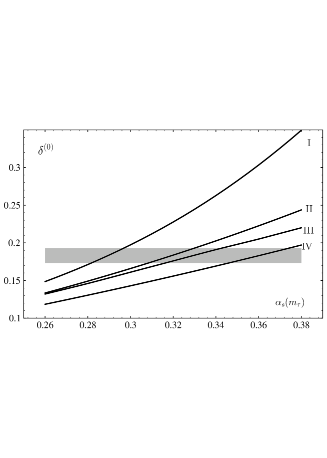
Figure 3: Perturbative corrections to the $\tau$ hadronic width. I: After resummation of one-loop running effects; II: Exact order $\alpha_{s}^{3}$-approximation; III: Exact order $\alpha_{s}^{3}$-approximation including the resummation of running coupling effects along a circle in the complex plane (taken from Pich); IV: Exact order $\alpha_{s}^{2}$-approximation for comparison. The shaded bar gives the experimental value with experimental errors only.

for the perturbative QCD corrections. In Fig. 3 we have plotted the prediction for $\delta^{(0)}$ as a function of $\alpha_{s}(m_{\tau})$ after resummation of one-loop running effects (recall for $R_{\tau}$ the exact $\alpha_{s}^{2}$- and $\alpha_{s}^{3}$-coefficients are very well approximated by one-loop running) as compared to the $\alpha_{s}^{2}$- and $\alpha_{s}^{3}$-approximation as well as the $\alpha_{s}^{3}$-approximation, including the resummation of [10]. We conclude that resummation of one-loop running reduces the central value for $\alpha_{s}(m_{\tau})$ by approximately 10% to

$$\alpha_{s}(m_{\tau})=0.29\,.$$ (3.17)

There is some difficulty in assigning an error to this value, which is related to the extent to which one trusts the restriction to one-loop running effects as a good estimate of higher order coefficients, not known exactly at present. In view of the fact that one-loop running overestimates the coefficient $d_{2}$ of $Q^{2}d\Pi/dQ^{2}$, one might consider $M_{\infty}^{\tau,\overline{\rm MS}}(a_{s})$ as an upper estimate for the effect of higher order perturbative corrections and the quoted value for $\alpha_{s}(m_{\tau})$ as a lower estimate for the central value. On the other hand, we shall see in Sect. 5.2, that a partial inclusion of two-loop running points towards even a lower value of $\alpha_{s}(m_{\tau})$. It seems safe to conclude that higher order corrections add up constructively and a cumulative effect is most likely to shift $\alpha_{s}(m_{\tau})$ towards the above value. Optimistically, one could even hope for a reduction of the theoretical uncertainty from the unknown residual perturbative corrections. A conservative evaluation would not exclude the entire region from 0.27 to 0.34 for $\alpha_{s}$ at the scale $m_{\tau}$. The lower bound reflects experimental and other than perturbative theoretical uncertainties and the upper bound follows from an analysis that takes into account only the completely known perturbative corrections up to cubic order.

The implications of the expected ultraviolet renormalon dominance for $R_{\tau}$ in large orders, which we have briefly touched upon above, have recently been investigated in Ref. [27], whose authors use conformal mapping techniques to construct the analytic continuation of the Borel transform beyond its radius of convergence set by the first ultraviolet renormalon. As noted in [27], such a technique is not particularly successful, when the series is not already close to the asymptotic ultraviolet renormalon behaviour (which is not the case for $R_{\tau}$ and $Q^{2}d\Pi/dQ^{2}$ up to cubic order), because then the intricate cancellations necessary to push the ultraviolet renormalon further away from the origin of the (conformally mapped) Borel plane than the first IR renormalon do not take place. The variation of results obtained from different mapping functions can then be considered analogous to the variations induced by different choices of renormalization schemes and as in the latter case it is difficult to decide to what extent such a (in principle arbitrary) variation should be considered as a theoretical error. Based on the evidence presented above, we believe that ultraviolet renormalons are sufficiently suppressed in fixed-order perturbative approximations to $R_{\tau}$ (but potentially not to $Q^{2}d\Pi/dQ^{2}$) to be safely ignored at present.

3.2 $(\Lambda_{\rm QCD}/m_{\tau})^{2}$-corrections

In this Subsection we investigate whether resummation of perturbative corrections can introduce power corrections, which elude the operator product expansion. We will exclude from the discussion the effect of renormalons, which have received main attention in this context [28, 11, 29, 14, 30, 27, 22]. As far as evidence from explicit calculations is available, infrared renormalons are in correspondence with condensates in the OPE as expected. There is no indication for explicit power corrections of dimension two from this source, which could turn out to be numerically significant. The effect of the dominant ultraviolet renormalon divergence is taken into account automatically by the error estimate due to unknown higher order perturbative corrections. After resummation it disappears completely in principle, although in practice this is not simple to implement [27] without approximations (like large $\beta_{0}$). It is also conceptually important to distinguish the statement that $1/Q^{2}$-corrections are absent in the OPE of correlation functions at euclidian momenta from that that $1/m_{\tau}^{2}$-corrections are absent in $R_{\tau}$. Validity of the first needs not imply the second, though the second will hardly be true without the first.

3.2.1 Definition of the coupling

Our first point of concern is the definition of the coupling parameter inherent to perturbative expansions and therefore to their resummations. To emphasize that this question is not connected with the minkowskian nature of $R_{\tau}$, we work with the derivative of the correlation function $D(Q^{2})$ rather than with $R_{\tau}$ itself.

Let us first take a closer look at the Borel sum (to be definite, let us assume a principal value prescription throughout this subsection, which corresponds to taking the real part of $r_{0}(\lambda_{L}^{2})$) in the representation as an integral over finite gluon mass in the large-$\beta_{0}$ (NNA) approximation. Let us denote the two terms on the right hand side of Eq. (2.24) by $I(\alpha_{s})$ for the integral and $L(\alpha_{s})$ for the contribution from the Landau pole in the dispersion relation for the running coupling (using the technique of Sect. 2.3 or [4]). The leading (two-loop) radiative correction with finite $\lambda$ can be obtained from the Borel transform by a Mellin transformation, see Eq. (2.16). Taking the integral analytically can be difficult, but for our present purpose we are interested only in the coefficients in the small-$\lambda^{2}$ expansion. This expansion can be obtained easily, since particular terms proportional to $(\lambda^{2}/m_{\tau}^{2})^{n}$ (modulo logarithms) correspond to contributions from singularities of the integrand in the right $u$-plane at $u=n$. For example, to pick up the term of order $\lambda^{2}/m_{\tau}^{2}$ one can evaluate the integrand in Eq. (2.16) at $u=1$, except for $\Gamma(-u)$. For the $D$-function defined in Eq. (3.8) we obtain

$$4\pi^{2}D(Q^{2},\lambda^{2}) = 1+\frac{\alpha_{s}}{\pi}\Bigg{\{}1-\left[\frac{32}{3}-8\zeta(3)\right]\frac{\lambda^{2}}{Q^{2}}-\left[2\ln(Q^{2}/\lambda^{2})+\frac{20}{3}-8\zeta(3)\right]\frac{\lambda^{4}}{Q^{4}}$$ (3.18)

$${}+O\left(\lambda^{6}\ln^{2}\lambda^{2}/Q^{2}\right)\Bigg{\}}\,.$$

The presence of quadratic terms, $\lambda^{2}/Q^{2}$, is not in conflict with the operator product expansion, since such terms come from the region of large momenta: As emphasized in Sect. 2.4, only non-analytic terms in the small $\lambda^{2}$-expansion can unambiguously be identified with infared contributions. The leading non-analytic term is proportional to $\lambda^{4}\ln\lambda^{2}$ and produces a correction proportional to $1/Q^{4}$, which can be related to the contribution of the gluon condensate [31] in the OPE. This contribution agrees with the calculation of the gluon condensate with finite gluon mass in [32], after the corresponding Wilson coefficient is extracted. (The difference in the constant $20/3$ arises, because we consider the derivative of $\Pi(Q^{2})$.).

The presence of a $\lambda^{2}/Q^{2}$-correction in Eq. (3.18) implies that the Landau-pole contribution in Eq. (2.24) is

$$L(\alpha_{s}(Q))\propto\exp\left(\frac{1}{\beta_{0}\alpha_{s}(Q)}\right)\propto\frac{\Lambda_{\rm QCD}^{2}}{Q^{2}}\,.$$ (3.19)

Numerically, this term is quite substantial. Taking $\alpha_{s}(Q)=0.32$ (which corresponds to $Q\simeq m_{\tau}$), separation of the two terms in Eq. (2.24) for $D(Q^{2})$ amounts to

$$M_{\infty}^{D}(0.229)=1.48=\mbox{integral over gluon mass}+0.31\,.$$ (3.20)

Note that $L(\alpha_{s})$ has identically vanishing perturbative expansion. Thus, without any additional information, keeping $I(\alpha_{s})$ alone in Eq. (2.24) provides an equally legitimate summation of the original series, which differs from Borel summation by terms of order $1/Q^{2}$, which are not related to renormalons or any particular regime of small or large momenta. We conclude, at this stage, that statements about power corrections are meaningful only with respect to particular summation prescriptions.

Physically, dropping the contribution $L(\alpha_{s})$ is equivalent to dropping the Landau pole contribution to the dispersion relation for the running coupling which can be interpreted as a redefinition of the coupling, such that the new coupling has no Landau pole. Since Borel summation in our limit of large $\beta_{0}$ coincides (in the V-scheme, $C$=0) with averaging the running coupling $\alpha_{s}(k)=\alpha_{s}(Q)/(1-\beta_{0}\alpha_{s}(Q)\ln(k^{2}/Q^{2}))$, it is readily seen from Eq. (2.33) that neglecting $L(\alpha_{s})$ corresponds to averaging with a coupling $\alpha^{\rm eff}_{s}(Q)$, related to $\alpha_{s}(Q)$ by

$$\alpha^{\rm eff}_{s}(Q)=\alpha_{s}(Q)-\frac{\lambda_{L}^{2}}{\beta_{0}(Q^{2}+\lambda_{L}^{2})}=\alpha_{s}(Q)-\frac{1}{\beta_{0}}\,e^{1/(\beta_{0}\alpha_{s}(Q))}+O\left(e^{2/(\beta_{0}\alpha_{s}(Q))}\right)\,.$$ (3.21)

This coupling has no Landau pole and freezes to a finite value as $Q^{2}$ approaches zero. However, it has $1/Q^{2}$-corrections to its evolution and correspondingly to the $\beta$-function:

$$\beta^{\rm eff}(\alpha_{s}^{\rm eff})=\beta_{0}(\alpha_{s}^{\rm eff})^{2}+\left(\frac{1}{\beta_{0}}+2\alpha_{s}^{\rm eff}\right)e^{1/(\beta_{0}\alpha_{s}^{\rm eff})}+O\left(e^{2/(\beta_{0}\alpha_{s}^{\rm eff})}\right)$$ (3.22)

Note that the absence of a Landau pole in $\alpha_{s}^{\rm eff}$ is seen only after summation of an infinite number of power corrections in $1/Q^{2}$ (exponentially small terms in $\alpha_{s}(Q)$) in Eq. (3.21). Further, the coefficients of perturbative expansions of any quantity are the same whether one uses $\alpha_{s}(Q)$ or $\alpha_{s}^{\rm eff}(Q)$ and diverge although the average

$$\int d^{4}k\,F(k,Q)\frac{\alpha^{\rm eff}_{s}(k)}{k^{2}}\sim I(\alpha_{s}(Q))$$ (3.23)

has no Landau pole ambiguities. We emphasize once more that averaging one-loop radiative corrections with this freezing coupling differs from Borel summation of the series in $\alpha_{s}(Q)$ (which gives $I(\alpha_{s}(Q))+L(\alpha_{s}(Q))$ by $1/Q^{2}$-terms. So does Borel summation of the identical series in $\alpha^{\rm eff}_{s}(Q)$, because the couplings differ by such terms. We shall argue that couplings like $\alpha_{s}^{\rm eff}(Q)$ obscure the relation to the operator product expansion in the sense that explicit $1/Q^{2}$-terms must be added to the resummed result (such as $L(\alpha_{s}(Q)$), had one used $\alpha_{s}^{\rm eff}(Q)$) in order to cancel spurious $1/Q^{2}$-effects in the large $Q^{2}$-expansion of the resummed result. This remark applies identically to a freezing coupling of type $1/(-\beta_{0}\ln(c+Q^{2}/\Lambda^{2}))$ and thus to the procedure of [6], where such a coupling has been used to estimate the size of infrared contributions for quantities related to heavy quark expansions.

We will now try to make precise the statement that $1/Q^{2}$-terms should be absent in the OPE. In order to talk about power corrections we have to attach some meaning to the divergent perturbative expansion at leading order in $1/Q^{2}$. A natural (though one might still ask whether it is justified to prefer Borel summation-type schemes to any other) definition apparently is

$$\left|D(Q^{2})_{\rm exact}-BS[D(\alpha_{s}(Q))_{\rm pert}]\right|\sim O\left(\frac{1}{Q^{4}}\right)\,,$$ (3.24)

where $BS[D(\alpha_{s}(Q))_{\rm pert}]$ denotes the Borel integral (with principal value prescription) of the perturbative expansion of $D$ in some $\alpha_{s}(Q)$. However, this statement is still ambiguous, because it implies knowledge of the $Q^{2}$-dependence in the coupling, which is arbitrary to a large extent. Moreover, it is not sufficient to appeal to the usual ambiguities in the choice of perturbative renormalization schemes, since the coupling and its evolution must be specified to power-like accuracy. We can bypass this point, noting that QCD with massless fermions has only a single free parameter. Since we are discussing asymptotic expansions in a dimensionful parameter $1/Q^{2}$, it seems most natural to choose a physical mass scale as this parameter, say $m_{\rho}^{2}$. This is especially natural in the context of lattice definitions of QCD, where one would trade the bare coupling for $m_{\rho}^{2}$. Then, if the operator product expansion exists nonperturbatively, this suggests the existence of a double expansion in $1/\ln(Q^{2}/m_{\rho}^{2})$ and $m_{\rho}^{2}/Q^{2}$ at large $Q^{2}$ and the interpretation of the statement that there are no $1/Q^{2}$ terms could be

$$\left|D(Q^{2})_{\rm exact}-BS[D(Q^{2})_{\rm pert}]\right|\leq K(\delta,R)\left(\frac{m_{\rho}^{2}}{cQ^{2}}\right)^{2}\,.$$ (3.25)

Here $BS[D(Q^{2})_{\rm pert}]$ denotes the Borel sum (with principal value prescription) of the leading term in the expansion of $D(Q^{2})$ at large $Q^{2}$, which is an infinite series in $1/\ln(cQ^{2}/m_{\rho}^{2})$, where $c$ is a constant to be specified later. The constant $K(\delta,R)$ depends on the opening angle $\delta$ and radius $R$ of the sector in the complex $1/Q^{2}$-plane, where Eq. (3.25) is supposed to hold. In general, $K(\delta,R)$ will neither be continuous nor bounded as a function of these two parameters. In particular, one can not expect a uniform bound in the entire cut plane. In the limit $\delta\rightarrow\pi$, this is related to violations of duality. We stress that as far as mathematical rigour is concerned, the validity of Eq. (3.25) must be regarded as purely hypothetical. We wish to present it as a mathematical formulation of the assumption that the operator product expansion holds at euclidian momenta (i.e. $\delta>0$) and no $1/Q^{2}$-terms are present in the asymptotic expansion. We note that the condition Eq. (3.25) is stronger than the condition that long-distance contributions can be factorized into condensates, which does not exclude the presence of power-like corrections, in particular $1/Q^{2}$, to coefficient functions, in particular of the unit operator, from short distances.

After we have chosen $m_{\rho}$ as the fundamental parameter of QCD, we may define the coupling by its beta-function and an overall scale. We define (again, to leading-$\beta_{0}$ accuracy)

$$\alpha_{s}(Q)=\frac{1}{-\beta_{0}\ln(cQ^{2}/m_{\rho}^{2})}\equiv\frac{1}{-\beta_{0}\ln(Q^{2}/\Lambda_{V}^{2})}\,,$$ (3.26)

where we have fixed $c$ by matching the large $Q^{2}$ behaviour with the $V$-scheme. It is easy to see that Eq. (3.25) implies Eq. (3.24) with this coupling, which by definition has no power-like evolution. This implication is not valid for couplings, that incorporate $1/Q^{2}$-dependence in their running. It is in this sense that we believe the use of freezing couplings is hazardous. If Eq. (3.25) is correct, then the use of Borel summation for perturbative series expressed in terms of such a coupling, or averaging lowest order radiative corrections with such a running coupling, necessitates the addition of explicit $1/Q^{2}$-corrections simply to cancel such corrections hidden in the definition of the coupling.

In practice, in one way or another, one relates physical quantities and an unphysical coupling like Eq. (3.26) might be considered as an intermediate concept only. However, the importance of being definite with the evolution of the coupling to power-like accuracy is not diminished by the use of physical couplings. To give a somewhat constructed example: If one expressed $R_{e^{+}e^{-}}$ as an expansion in the effective coupling, defined by QCD corrections to the Gross-Llewellyn-Smith sum rule, one would expect $1/Q^{2}$-corrections to this perturbative relation, which are imported from the definition of the coupling.

3.2.2 Analyticity and the Landau pole

After renormalization group improvement, perturbative expansions are plagued by the Landau pole. This unphysical singularity is endemic not only to perturbative expansions, but to the operator product expansion, truncated to any finite order. It requires some care in defining resummations for quantities like $R_{\tau}$, which are related to euclidian quantities by analyticity. For the purpose of illustration, we shall restrict ourselves to the approximation, where $\beta(\alpha_{s})=\beta_{0}\alpha_{s}^{2}$ and adopt the V-scheme, $C=0$, in all explicit formulas. Then, ignoring an irrelevant $Q^{2}$-independent subtraction, we can write the Borel sum (with principal value prescription, as usual) as

$$BS[\Pi](Q^{2}) \equiv \frac{1}{-\beta_{0}}\int\limits_{0}^{\infty}du\,e^{-u/(-\beta_{0}\alpha_{s}(\mu))}B[\Pi](u,Q^{2}/\mu^{2})=\frac{1}{-\beta_{0}}\int\limits_{0}^{\infty}du\left(\frac{\Lambda_{V}^{2}}{Q^{2}}\right)^{u}F(u)$$ (3.27)

$$= BS[\Pi]_{<}(Q^{2},u_{0})+BS[\Pi]_{>}(Q^{2},u_{0})\,,$$

where we use $\alpha_{s}(Q)=1/(-\beta_{0}\ln(Q^{2}/\Lambda^{2}_{V}))$ and $F(u)$ is $Q^{2}$-independent. In the second line, we have defined two new functions by splitting the Borel integral into two regions from 0 to $u_{0}$ and $u_{0}$ to $\infty$. From the explicit form in Eq. (3.9), we deduce that, for any (positive) $u_{0}$, $BS[\Pi]_{<}(Q^{2},u_{0})$ is analytic in the $Q^{2}$-plane cut along the negative axis. On the other hand the $u$-integral in $BS[\Pi](Q^{2})$ diverges, when $Q^{2}<\Lambda_{V}^{2}$ and $Q^{2}=\Lambda^{2}_{V}$ is a singular point. We say that $BS[\Pi](Q^{2})$ has a Landau pole, though, in general, $Q^{2}=\Lambda^{2}_{V}$ will rather be a branch point.

Notice, since in practice one truncates the operator product expansion at operators of some dimension $d$, it is perfectly consistent to replace $BS[\Pi](Q^{2})$ by $BS[\Pi]_{<}(Q^{2},u_{0})$, provided we choose $u_{0}>d/2+1$, since the difference is bounded by

$$\left|BS[\Pi](Q^{2})-BS[\Pi]_{<}(Q^{2},u_{0})\right|<\tilde{K}(R)\left(\frac{\Lambda_{V}^{2}}{Q^{2}}\right)^{u_{0}}$$ (3.28)

and vanishes faster than other corrections neglected in the truncation of the OPE. In this case, the bound can be established in a cut circle of radius $R$ in the $1/Q^{2}$-plane. Again, it will not be possible to establish uniform bounds, since typically $\tilde{K}(R)\sim 1/\ln(R\Lambda_{V}^{2})$. Thus, although for fixed $Q^{2}>1/R$, the difference can be made vanish faster than any desired power of $\Lambda_{V}^{2}/Q^{2}$ by increasing $u_{0}$, at fixed $u_{0}$ the bound may become arbitrarily weak as $Q^{2}$ approaches $\Lambda_{V}^{2}$. Still, we conclude that the presence or absence of a Landau pole in resummed results is related to the behaviour of the Borel integral at infinity and is thus an effect that formally vanishes faster than any power of $1/Q^{2}$.

Consider now the two different representations for the tau decay width, Eqs. (3) and (3.5), in this light. We use equality of vector and axial-vector correlators in perturbation theory and abbreviate the weight function by $w(s/m_{\tau}^{2})$. Then

$$R_{\tau}^{\mbox{{\tiny eq.(\ref{rep1})}}}=24\pi\int\limits_{0}^{m_{\tau}^{2}}\frac{ds}{m_{\tau}^{2}}\,w\!\left(\frac{s}{m_{\tau}^{2}}\right)\,\frac{1}{2i}\mbox{disc}\,BS[\Pi](s)\,,$$ (3.29)

$$R_{\tau}^{\mbox{{\tiny eq.(\ref{rep2})}}}=12\pi i\int\limits_{|s|=m_{\tau}^{2}}\frac{ds}{m_{\tau}^{2}}\,w\!\left(\frac{s}{m_{\tau}^{2}}\right)\,BS[\Pi](s)\,.$$ (3.30)

Note that in both cases summation is carried out inside the $s$-integral. The following considerations can easily be extended to the situation, where summation is taken after $s$-integration (and do not lead to any of the differences observed below). We define $R_{\tau,<}^{\mbox{{\tiny eq.(\ref{rep1})}}}(u_{0})$ and $R_{\tau,<}^{\mbox{{\tiny eq.(\ref{rep2})}}}(u_{0})$ by the replacement of $BS[\Pi](s)$ by $BS[\Pi]_{<}(s,u_{0})$. Using the analyticity properties discussed above as well as $m_{\tau}^{2}>\Lambda_{V}^{2}$, it is straightforward to find

$$R_{\tau}^{\mbox{{\tiny eq.(\ref{rep2})}}}-R_{\tau,<}^{\mbox{{\tiny eq.(\ref{rep2})}}}(u_{0})\sim\left(\frac{\Lambda_{V}^{2}}{m_{\tau}^{2}}\right)^{u_{0}}\qquad R_{\tau,<}^{\mbox{{\tiny eq.(\ref{rep1})}}}(u_{0})=R_{\tau,<}^{\mbox{{\tiny eq.(\ref{rep2})}}}(u_{0})\,,$$ (3.31)

but

$$R_{\tau}^{\mbox{{\tiny eq.(\ref{rep1})}}}-R_{\tau}^{\mbox{{\tiny eq.(\ref{rep2})}}}=-12\pi i\int\limits_{C}\frac{ds}{m_{\tau}^{2}}\,w\!\left(\frac{s}{m_{\tau}^{2}}\right)\,BS[\Pi]_{>}(s,u_{0})\,,$$ (3.32)

where the contour $C$ runs along a circle of radius $\Lambda_{V}^{2}$ around $s=-\Lambda_{V}^{2}$. Against appearances, the right hand side is independent of $u_{0}$. Of course, one can not take $u_{0}$ to infinity inside the integral and conclude that it is zero. $BS[\Pi]_{>}(s,u_{0})$ has a pole or branch point at $s=-\Lambda_{V}^{2}$ and we find

$$R_{\tau}^{\mbox{{\tiny eq.(\ref{rep1})}}}-R_{\tau}^{\mbox{{\tiny eq.(\ref{rep2})}}}\sim\frac{\Lambda_{V}^{2}}{m_{\tau}^{2}}$$ (3.33)

and similarly

$$R_{\tau}^{\mbox{{\tiny eq.(\ref{rep1})}}}-R_{\tau,<}^{\mbox{{\tiny eq.(\ref{rep1})}}}(u_{0})\sim\frac{\Lambda_{V}^{2}}{m_{\tau}^{2}}\,.$$ (3.34)

Since Eq. (3.28) is not valid for $s<\Lambda_{V}^{2}$, this result should not surprise. The difference in Eq. (3.33) arises, because the resummation introduces (or preserves) the Landau pole singularity, which is in conflict with the analytic properties of the exact correlation function, that have been assumed to derive Eq. (3.5) from Eq. (3).

Should one conclude then that resummations of perturbative corrections are ambiguous by terms of order $1/m_{\tau}^{2}$, even if there are no $1/Q^{2}$ terms in the OPE at euclidian momenta in the strong sense of Eq. (3.25)? Do we have evidence for power corrections not captured by the OPE, since they originate from $u=\infty$ in the Borel integral? The answer is no. A positive answer would be warranted, if there were no reason to prefer the prescription Eq. (3.29) to Eq. (3.30) or vice versa, while only the second can be used. The reason is that the region $|s|<\Lambda_{V}^{2}$ can not be penetrated to any finite order in the short distance expansion ($1/Q^{2}$-expansion). Since all summation prescriptions of perturbative expansions are formulated within the context of the short-distance expansion, they can not be applied to $|s|<\Lambda_{V}^{2}$, unless the summation of this expansion itself is understood. This discards Eq. (3.29) as a legitimate summation. One must first use the analyticity properties of the exact correlation functions to deform the contour outside the region $|s|<\Lambda_{V}^{2}$, before an attempt at summing perturbative expansions can be made, which privileges Eq. (3.5) as the starting point. A different way to express this fact is to observe that the principal value Borel integral is defined for $|s|<\Lambda_{V}^{2}$ only in the sense of analytic continuation, but cannot be used as a numerical approximation since all power corrections in the operator product expansion are of the same order of magnitude in this region. It is only when all these are taken into account that the Landau pole vanishes in physical observables.

To conclude this Section, let us mention that a relation between analyticity in $s$ and behaviour of the Borel integral at infinity has been noted in a very different and much more physical context in [33]. The presence of resonances and multiple thresholds on the physical axis was observed to be in conflict with Borel summation. In this case, the restoration of the correct analytic properties should also be understood in connection with summing the OPE itself [35]. A much more elaborate argument has been presented in [36], where the presence of resonances was connected with the divergence of OPE, which also offers a way to understand the concept of duality and its limitations. If the OPE is by itself only an asymptotic expansion, it is quite possible that its application is limited to a finite phase range in the complex $s$-plane around the negative $s$-axis. We believe that this possibility should be taken seriously, since it might imply the presence of $1/s_{0}$-corrections in finite averages up to $s_{0}$ of the discontinuity along the physical axis (for $R_{\tau}$, $s_{0}=m_{\tau}^{2}$). Unfortunately, we do not know how to substantiate or disprove such a statement theoretically.

4 The pole mass of a heavy quark

Although on-shell quarks do not exist and there is presumably no natural nonperturbative definition of a pole mass of a quark, the pole mass has proven useful as an auxiliary concept in applications of perturbative QCD to heavy quark physics, where physically the quark is expected to be close to its would-be mass-shell. Still, the relation between the pole mass and an off-shell renormalized mass is known to have large perturbative coefficients from small loop momenta, at least in high orders of perturbation theory [17, 37]. Since neither quark mass definition is physical, this might appear as an irrelevant problem. However, the behaviour of perturbative expansions of quantities involving quark masses change accordingly with the quark mass definition used and in general one expects coefficients to be significantly reduced, when the pole mass is abandoned in favour of an off-shell renormalized mass [37, 20], such as $\overline{\rm MS}$. In the latter case, it is quite well-known that the exact two-loop coefficient [38] in the relation to the pole mass is substantial and one might wonder whether this is coincidental.

In this Section we apply resummation and NNA to the difference between the pole and $\overline{\rm MS}$ mass. Apart from its practical interest, we also use this quantity to illustrate certain features of higher order perturbative corrections, when the masses of fermions in loops are finite. The reader interested only in results may jump directly to Sect. 4.3, where our best estimate is presented. In this Section $\alpha_{s}(\mu)$ always refers to the $\overline{\rm MS}$ coupling.

4.1 Preliminaries

To begin with, let us quote the exact two-loop result from [38]:

$$\frac{\delta m}{m}\equiv\frac{m_{\rm pole}-m_{\overline{\rm MS}}(m_{\overline{\rm MS}})}{m_{\overline{\rm MS}}(m_{\overline{\rm MS}})}=\frac{4}{3}\frac{\alpha_{s}(m_{\overline{\rm MS}})}{\pi}\left[1+\left(4.68\,(-\beta_{0}^{N_{f}})-\left\{\begin{array}[]{c}0.89\\ 0.91\end{array}\right\}\right)\alpha_{s}(m_{\overline{\rm MS}})\right]$$ (4.1)

The upper entry in curly brackets refers to the calculation with $N_{f}$ massless quarks and a quark of mass $m$ in loops, the lower entry to the situation, where the quark flavour of mass $m$ is excluded from loops. The superscript on $\beta_{0}$ indicates the value of $N_{f}$ to be taken for the $\beta$-function. Since $(-\beta_{0}^{N_{f}})\sim 2/3$ for cases of interest, $N_{f}=3,4$, we note that keeping the term proportional to $\beta_{0}^{N_{f}}$ alone provides indeed a reasonable approximation within $30-40\%$ of the exact coefficient.

Note that above we have normalized $m_{\overline{\rm MS}}$ at the scale $m_{\overline{\rm MS}}$, since we prefer to eliminate $m_{\rm pole}$ in all places. When Eq. (4.1) is expressed in terms of the $\overline{\rm MS}$ mass normalized at $m_{\rm pole}$,

$$\frac{m_{\rm pole}-m_{\overline{\rm MS}}(m_{\rm pole})}{m_{\overline{\rm MS}}(m_{\rm pole})}=\frac{4}{3}\frac{\alpha_{s}(m_{\rm pole})}{\pi}\left[1+\left(4.68\,(-\beta_{0}^{N_{f}})-\left\{\begin{array}[]{c}0.25\\ 0.28\end{array}\right\}\right)\alpha_{s}(m_{\rm pole})\right]\,$$ (4.2)

the approximation of keeping only the term proportional to $\beta_{0}^{N_{f}}$ is significantly improved. This ambiguity is in fact a source of trouble within the BLM and our extended prescription. For $\delta m$ additional renormalization scheme and scale dependence is present from the definition of the quark mass parameter, whereas the BLM method by construction deals only with the scale-dependence of the coupling. Although the calculation of fermion loop insertions and subsequent restoration of $\beta_{0}$ also provides the anomalous dimension of the quark mass within the same approximation, the scheme ambiguity in the size of neglected genuine two-loop corrections is amplified by this additional source of scheme-dependence. If $\mu_{1}^{2}-\mu_{2}^{2}\sim O(\alpha_{s})$, then the difference $m_{\overline{\rm MS}}(\mu_{1})-m_{\overline{\rm MS}}(\mu_{2})$ must be neglected in the approximation of large $\beta_{0}$, although it can be sizeable, if the coefficient of $\alpha_{s}$ in $\mu_{1}^{2}-\mu_{2}^{2}$ is so. In the following, we will work with Eq. (4.1), whenever relevant.

Let us first consider the (excellent) approximation, that the quark flavour of mass $m$ is neglected in loops. All other $N_{f}$ quarks are massless. In this case the relevant $\beta$-function coefficient is $\beta_{0}^{N_{f}}$ and an exact expression for the Borel transform of the mass shift exists [17]:

$$B\left[\delta m/m\right](u)=\frac{1}{3\pi}\left[e^{5u/3}\,6(1-u)\frac{\Gamma(u)\Gamma(1-2u)}{\Gamma(3-u)}+\frac{\tilde{G}_{0}(u)}{u}\right]$$ (4.3)

$\tilde{G}_{0}(u)$ is defined in the following way (see Appendix A): If $g_{n}$ are the expansion coefficients of $G_{0}(u)$ in $u$, then $\tilde{G}_{0}(u)$ has expansion coefficients $g_{n}/n!$. $G_{0}(u)$ can be calculated with the methods of Appendix A and is found to be

$$G_{0}(u)=-\frac{1}{3}(3+2u)\frac{\Gamma(4+2u)}{\Gamma(1-u)\Gamma^{2}(2+u)\Gamma(3+u)}\,.$$ (4.4)

Higher order perturbative corrections with fermion loop insertions into the one-loop diagram can then be computed according to Eq. (2.7). Equivalently, one can start from Eq. (2.28) with the input of the one-loop mass shift with finite gluon mass, given by ($x\equiv\lambda^{2}/m^{2}$)

$$r_{0}(\lambda^{2}) = \frac{1}{3\pi}\Bigg{[}4+x-\frac{x^{2}}{2}\ln x-\frac{\sqrt{x}(8+2x-x^{2})}{\sqrt{4-x}}\Bigg{\{}\arctan\left[\frac{2-x}{\sqrt{x(4-x)}}\right]+$$ (4.5)

$$\,\arctan\left[\frac{\sqrt{x}}{\sqrt{4-x}}\right]\Bigg{\}}\Bigg{]}=\frac{4}{3\pi}\left[1+\frac{\pi}{2}\sqrt{x}+\frac{3}{4}x+O\left(x^{3/2}\right)\right]\,.$$

We define coefficients $d_{n}$ as in Sect. 2 by

$$\frac{\delta m}{m}=\frac{4}{3}\frac{\alpha_{s}(m)}{\pi}\left[1+\sum_{n=1}^{\infty}d_{n}\,(-\beta_{0}^{N_{f}}\alpha_{s}(m))^{n}\right]\,.$$ (4.6)

They are listed in Table 2. Higher order perturbative corrections grow very rapidly, as expected from the dominant asymptotic behaviour from the pole at $u=1/2$ in Eq. (4.3),

$$d_{n}\stackrel{{\scriptstyle n\gg 1}}{{=}}e^{5/6}\,2^{n}n!\,.$$ (4.7)

$$\begin{array}[]{|c||c|c|c|}\hline\cr n&d_{n}&M_{n}\,[\mbox{c-quark}]&M_{n}\,[\mbox{b-quark}]\\ \hline\cr\hline\cr 0&1&1&1\\ 1&4.6861511&2.176&1.623\\ 2&17.622650&3.286&1.935\\ 3&109.85885&5.024&2.193\\ 4&873.92393&8.492&2.467\\ 5&8839.6860&17.30&2.835\\ 6&105814.28&43.76&3.420\\ 7&1484968.4&137.0&4.514\\ 8&237407365&511.0&6.838\\ \hline\cr\infty&-&1.712\pm 0.608&2.041\pm 0.201\\ \hline\cr m^{*}_{1}&-&0.096\,m_{c}&0.096\,m_{b}\\ m^{*}_{\infty}&-&0.437\,m_{c}&0.147\,m_{b}\\ \hline\cr\end{array}$$

Table 2: Higher order perturbative corrections to the difference between the pole and $\overline{\rm MS}$ mass from $n$ fermion loop insertions. The second and third columns give partial sums and summations for the charm quark ($a_{s}=-\beta_{0}^{(3)}\alpha_{s}(m_{c})=0.251$) and bottom quark ($a_{s}=-\beta_{0}^{(4)}\alpha_{s}(m_{b})=0.133$). In the latter case, the c-quark is treated as massless inside loops.

This asymptotic formula is in fact a very good approximation (within 5%) to the exact coefficient $d_{n}$ for all $n\geq 1$, which seems to imply that the saddle point approximation of the loop momentum distribution inherent to deriving the asymptotic behaviour is a very good substitute for the exact distribution, even if the width of the Gaussian is not small. Given that genuine two-loop corrections are rather small compared to $d_{1}$, it can be asserted that the exact two-loop coefficient is already dominated by the first infrared renormalon at $u=1/2$. Evidently, this observation is scheme-dependent and we do not know why the $\overline{\rm MS}$ scheme is preferred. Let us note, however, that a similar coincidence can not be expected and indeed does not happen (see Sect. 3) for quantities, whose asymptotic behaviour is dominated by ultraviolet renormalons, like $R_{e^{+}e^{-}}$ or $R_{\tau}$, since with $C=-5/3$ in the $\overline{\rm MS}$ scheme, the leading ultraviolet singularity at $u=-1$ is suppressed compared to the leading infrared singularity at $u=2$ by a factor $e^{-5}\approx 7\cdot 10^{-3}$. Therefore the latter is expected to dominate in intermediate orders [35] (if there is any regularity at all) and it might not be an accident, that exact low order coefficients are indeed of same sign for these quantities.

Table 2 also shows how the one-loop radiative correction to the pole mass is modified by inclusion of a finite number of fermion loops and by summation according to Eq. (2.29). We have taken $\alpha_{s}(m_{b})=0.2$ and $\alpha_{s}(m_{c})=0.35$. Recall that the sum corresponds to a principal value prescription for the Borel integral. The errors quoted correspond to the imaginary part of the Borel integral, when it is defined by deforming the contour into the complex plane. The imaginary part can be taken as an estimate of inherent uncertainty of perturbative relations. We have actually divided this imaginary part by $\pi$, which upon inspection we find closer to, but somewhat smaller than the naive estimate of uncertainty by the minimal term of the series. A more conservative estimate would be to enlarge these errors by a factor of two. The BLM scales in Table 2 are defined by (cf. Eq.(1.5))

$$m^{*}_{1}=m\,\exp\left[-\frac{1}{2a_{s}}(M_{1}(a_{s})-1)\right]\,,\qquad m^{*}_{\infty}=m\,\exp\left[-\frac{1}{2a_{s}}\left(1-\frac{1}{M(a_{s})}\right)\right]\,.$$ (4.8)

The uncertainty in $M_{\infty}(a_{s})$ translates into an uncertainty of the BLM scale $m^{*}_{\infty}$ by the previous equation. We want to point out that the usual BLM scale $m^{*}_{1}$, which uses only $d_{1}$ as input is smaller than $m^{*}_{\infty}$ although all higher orders $d_{n}$ add up positively. The reason is that $\alpha_{s}(m^{*}_{1})$ upon re-expanding in terms of $\alpha_{s}(m)$ implies $d_{n}^{\rm BLM}=d_{1}^{n}$. For the charm and bottom quark mass the most important effect comes from $n=1,2$. But since $d_{1}$ is rather large, $d^{\rm BLM}_{2}=d_{1}^{2}\approx 21.9>17.6=d_{2}$, and the usual BLM prescription overestimates the size of radiative corrections. This behaviour is quite generic to quantities dominated by scales below a few GeV and with a leading infrared renormalon at $u=1/2$.

4.2 Effect of internal quark masses

Before proceeding to realistic charm and bottom quarks we want to illustrate the effect of finite quark masses inside loops on the coefficients of diagrams with quark loop insertions in the toy example of the mass shift due to a single quark flavour with mass $m_{i}$ in loops. The “heavy” quark of mass $m$ is again excluded from loops.

The factorially large contribution from small and large loop momenta can be traced to the logarithmic behaviour of the vacuum polarization for a massless particle at very small and very large virtuality. In the case of small virtuality, the large coefficient arises from momenta $k\sim me^{-n}\ll m$. For a massive quark the logarithmic behaviour is cut off, because at very small momenta its vacuum polarization is proportional to $k^{2}/m_{i}^{2}$. Thus, no matter how small the quark mass, the factorially large contribution should be eliminated when $n$ is such that $me^{-n}<m_{i}$. There are no infrared renormalon singularities in the Borel transform in the absence of massless particles. This expectation is verified in Fig. 4, where we have plotted the ratio of the coefficient $d_{n}(m_{i})$, computed with internal mass $m_{i}$, and $d_{n}(0)$ for the massless case as in Table 2 as a function of the number of loops $n$ for various ratios of $m_{i}/m$. Since $m_{i}$ serves effectively as an infrared cutoff, Fig. 4 provides some information on what proportion of the coefficient $d_{n}(0)$ originates from low momentum regions. Note that low momentum means low momentum compared to $m$ and not $\Lambda_{\rm QCD}$. Eventually, as $n$ becomes large, coefficients will be dominated by large momentum for any $m_{i}$ and the asymptotic behaviour of Eq. (4.7) is replaced by a sign-alternating behaviour due the leading ultraviolet renormalon

Figure 4: Ratio $d_{n}(m_{i})/d_{n}(0)$ for different values of internal quark masses $m_{i}$ as a function of the number of fermion loop insertions. The value of $m_{i}^{2}/m^{2}$ is indicated to the right of each curve.

$$d_{n}(m_{i})\stackrel{{\scriptstyle n\gg 1}}{{=}}\left[-1+\frac{9}{2}\frac{m_{i}^{2}}{m^{2}}\right]e^{-5/3}\,(-1)^{n}n!\,.$$ (4.9)

We find that for $m_{i}^{2}/m^{2}\geq 0.1$, this asymptotic behaviour practically coincides with the exact coefficient for $n>6$.

The presence of mass dependence in the coefficient of ultraviolet renormalons requires some explanation. The singularity of the Borel transform at $u=-1$, which is responsible for Eq. (4.9), is due to the presence of a $1/k^{6}$-term in the expansion of the Feynman integrand for the one-loop mass-shift at large $k$:

$$\delta m\sim\alpha_{s}\,m\int d^{4}k\left(\frac{a}{k^{4}}+b\frac{m^{2}}{k^{6}}+\ldots\right)$$ (4.10)

The $1/k^{4}$-term creates a logarithmic ultraviolet divergence, which is subtracted by minimal subtraction. The effect of the Borel transformed gluon propagator (with fermion loop insertions) amounts to insertion of (see Sect. 2.3)

$$\exp(-u\Pi(k^{2})/a_{s})=\left(-\frac{m^{2}}{k^{2}}e^{-C}\right)^{\!u}\left[1+6u\frac{m_{i}^{2}}{k^{2}}+O\left(\frac{m_{i}^{4}}{k^{4}}\right)\right]$$ (4.11)

into the integrand. The pole at $u=-1$ arises, because close to $u=-1$ the $1/k^{6}$-term is converted into a logarithmically divergent term. But when $m_{i}$ is not zero a second contribution of order $1/k^{6}$ arises, when $a/k^{4}$ combines with the first mass correction in Eq. (4.11). This term accounts for the mass-dependence of ultraviolet renormalons in minimal subtraction schemes. Had one chosen a renormalization prescription, which subtracts the $a/k^{4}$-term inside the integrand, that mass-dependence would be absent for the first ultraviolet renormalon at $u=-1$, but still present in coefficients of singularities at $u=-2,-3\ldots$.

4.3 Charm and bottom pole masses

For realistic charm and bottom quarks, the numerical results of Sect. 4.1 need to be amended in two respects: The quark, whose mass shift is considered, should also be taken into account in loops. This effect is tiny, but we include it for completeness. More interesting is the effect of finite charm mass on the bottom pole mass, because the charm mass might be larger than the typical loop momentum already in low orders. If so, it would seem more appropriate to use $\beta_{0}^{(3)}$ rather than $\beta_{0}^{(4)}$, when restoring the QCD $\beta$-function coefficient from the calculation of fermion loops. Strictly speaking, changing the mass of one flavour is a negligible effect in the formal large-$\beta_{0}$ limit (i.e. large-$N_{f}$), and should be discarded in a consistent approximation. In realiter the effect is numerically noticeable and we prefer to include it as a calculable correction, keeping in mind its size as an uncertainty in our approach.

To gain some understanding of the numerical results to follow, we trace the decoupling of internal charm loops for the bottom pole mass in more detail. For this purpose, we ignore again the bottom quark in loops. When the order of perturbation theory is sufficiently large, internal integrations are dominated by momenta much smaller than $m_{c}$. Let us denote coefficients including charm loops by $d_{n}^{[3+1]}(m_{c})\,(-\beta_{0}^{(4)})^{n}$ and those without charm loops by $d_{n}^{[3]}\,(-\beta_{0}^{(3)})^{n}$. Then one might expect

$$d_{n}^{[3+1]}(m_{c})\,\left(-\beta_{0}^{(4)}\right)^{n}\alpha_{s}(m_{b})^{n+1}\approx d_{n}^{[3]}\,\left(-\beta_{0}^{(3)}\right)^{n}\alpha_{s}(m_{b})^{n+1}$$ (4.12)

if $n$ is sufficiently large up to corrections suppressed by a power of the typical internal momentum divided by $m_{c}$. This is not quite correct, because there is no manifest decoupling in the $\overline{\rm MS}$ scheme. In the limit that we consider only the contribution from small $\lambda^{2}$, appropriate for sufficiently large $n$, the Borel transform including the massive charm in Eq. (2.37) reduces to

$$B\left[\frac{\delta m}{m}\right](u)=\exp\!\left(\frac{u}{6\pi\beta_{0}^{(4)}}\ln\frac{\mu^{2}}{m_{c}^{2}}\right)\!\left(-\frac{1}{\pi}\right)\sin\!\left(\frac{u\beta_{0}^{(3)}}{\beta_{0}^{(4)}}\right)\!\!\int\limits_{0}^{\infty}\frac{d\lambda^{2}}{\lambda^{2}}\,(r_{0}(\lambda^{2})-r_{0}(0))\!\left(\frac{\lambda^{2}}{\mu^{2}e^{5/3}}\right)^{\!\!u\beta_{0}^{(3)}/\beta_{0}^{(4)}}$$ (4.13)

up to power corrections. If the first factor were absent, this Borel transform would coincide with the one for purely massless flavours up to a rescaling of $u$ which is just what is necessary to obtain Eq. (4.12) from Eq. (2.7). The first factor is present, because the vacuum polarization for charm has been renormalized in the $\overline{\rm MS}$ scheme and not by zero momentum subtraction, which would lead to manifest decoupling. The difference can be accomodated by a change of the coupling constant. This is most easily seen by combining the extra exponential factor with the exponential in the Borel integral, Eq. (2.8). We deduce that (up to power corrections in the typical loop momentum divided by $m_{c}$)

$$d_{n}^{[3+1]}(m_{c})\,\left(-\beta_{0}^{(4)}\right)^{n}\alpha_{s}^{(4)}(m_{b})^{n+1}\approx d_{n}^{[3]}\,\left(-\beta_{0}^{(3)}\right)^{n}\alpha_{s}^{(3)}(m_{b})^{n+1}\,,$$ (4.14)

where the two couplings are related by

$$\frac{1}{\alpha_{s}^{(3)}(\mu)}=\frac{1}{\alpha_{s}^{(4)}(\mu)}+\frac{1}{6\pi}\,\ln\frac{\mu^{2}}{m_{c}^{2}}\,.$$ (4.15)

Alternatively, we can simply replace $u$ in the extra exponential factor in Eq. (4.13) by the location of the closest infrared pole of the Borel transform, $u=1/2$, and obtain 3,4

$$d_{n}^{[3+1]}(m_{c})\,\left(-\beta_{0}^{(4)}\right)^{n}\alpha_{s}(m_{b})^{n+1}\approx\exp\left(\frac{1}{12\pi\beta_{0}^{(4)}}\ln\frac{m_{b}^{2}}{m_{c}^{2}}\right)d_{n}^{[3]}\,\left(-\beta_{0}^{(3)}\right)^{n}\alpha_{s}(m_{b})^{n+1}\,,$$ (4.16)

which is equivalent to Eq. (4.14) for large $n$.

$$\begin{array}[]{|c||c|c|c|c|}\hline\cr n&d_{n}^{[3]}&d_{n}^{[3+1]}&d_{n}^{[3]}\,(\beta_{0}^{(3)}/\beta_{0}^{(4)})^{n}&M_{n}^{[3+1]}\\ \hline\cr\hline\cr 0&1&1&1&1\\ 1&4.6862&5.0984&5.0613&2.183\\ 2&17.623&20.514&20.555&3.291\\ 3&109.86&138.58&138.38&5.021\\ 4&873.92&1188.3&1189.0&8.470\\ \hline\cr\infty&-&-&-&1.720\pm 0.608\\ \hline\cr m^{*}_{1}&-&-&-&0.078\,m_{c}\\ m^{*}_{\infty}&-&-&-&0.406\,m_{c}\\ \hline\cr\end{array}$$

Table 3: Perturbative corrections to the pole charm quark mass with (column 3) and without (column 2) charm inside loops. For comparison, column 4 gives coefficients in the limit that all internal masses are large compared to the typical loop momentum. The last column updates the modification of one-loop corrections due to coefficients $d_{n}^{[3+1]}$.

$$\begin{array}[]{|c||c|c|c|c|}\hline\cr n&d_{n}^{[3]}&d_{n}^{[3+2]}&K\,d_{n}^{[3]}\,(\beta_{0}^{(3)}/\beta_{0}^{(5)})^{n}&M_{n}^{[3+2]}\\ \hline\cr\hline\cr 0&1&1&1&1\\ 1&4.6862&5.3093&4.9774&1.648\\ 2&17.623&22.720&21.975&1.986\\ 3&109.86&159.69&160.82&2.276\\ 4&873.92&1.5\cdot 10^{3}&1502.0&2.601\\ \hline\cr\infty&-&-&-&2.099\pm 0.224\\ \hline\cr m^{*}_{1}&-&-&-&0.064\,m_{b}\\ m^{*}_{\infty}&-&-&-&0.117\,m_{b}\\ \hline\cr\end{array}$$

Table 4: Coefficients as in the previous table, where $d_{n}^{[3+2]}$ now includes charm and bottom masses with $m_{c}^{2}/m_{b}^{2}=0.1$. $K=\exp(1/(12\pi\beta_{0}^{(5)})\ln(m_{b}^{2}/m_{c}^{2}))\approx 0.9$.

Numerical values for corrections to the charm pole mass and the bottom pole mass, including the charm and bottom masses in loops, are given in Tables 3 and 4. For the bottom pole mass, the result depends only on the ratio $m_{c}/m_{b}$ and we used $m_{c}^{2}/m_{b}^{2}=0.1$. For comparison coefficients according to Eq. (4.16) are given. The last column in both tables displays the modification of the one-loop mass shift by running coupling effects. Note that at the charm scale, the perturbative series has to be truncated already at second order. The lower rows give the result of summation according to Eq. (2.37) and the corresponding BLM scales, Eq. (4.8). Two technical observations are in order: First, as mentioned in Section 2, the sum as defined by Eq. (2.37) does not exactly coincide with the principal value of the Borel integral. The difference is tiny for the value of masses considered here and does not affect our conclusions which are based on the behaviour of perturbation theory in low and intermediate orders. Second, for the bottom quark the BLM scale is defined without taking into account the charm threshold in the running coupling.

The difference between the pole mass and the $\overline{\rm MS}$-renormalized mass (normalized at $m_{\overline{\rm MS}}$) for bottom quarks can now be written as

$$\frac{\delta m_{b}}{m_{b}}=\frac{4}{3}\frac{\alpha_{s}(m_{b})}{\pi}\left[M_{\infty}^{[3+2]}(-\beta_{0}^{(5)}\alpha_{s}(m_{b}))-0.91\alpha_{s}(m_{b})+\mbox{higher orders}\right]\,,$$ (4.17)

where the second term in square brackets accounts for the genuine gluonic two-loop corrections, cf. Eq. (4.1). Unknown higher order corrections include genuine three- and higher loop corrections, vacuum polarization insertions into two-loop corrections as well as effects of two-loop running on lowest order radiative corrections. Numerically, for $\alpha_{s}(m_{b})=0.2$, we find

$$\frac{\delta m_{b}}{m_{b}}=(16.3\pm 2.9\pm 1.5)\%\,.$$ (4.18)

Compared to the two-loop expression, the estimate obtained from NNA increases the mass shift from about $12\%$ to $16\%$. The second error reflects our estimate of unknown higher order corrections, which we allow to be as large as the genuine two-loop corrections. The first error, which dominates the total uncertainty, represents an estimate of the ultimate accuracy of $\delta m_{b}/m_{b}$ due to the divergence of the perturbative series. It can not be reduced by calculating higher orders (but of course refined – the numerical value we quote has been obtained by increasing the uncertainty of $M_{\infty}^{[3+2]}(a_{s})$ in Table 4 by 50%, upon which it is close to the minimal term of the series at $n\approx 2-3$). In absolute values, the intrinsic uncertainty of $\delta m_{b}$ and therefore of the pole mass of the bottom quark ranges between $100$ and $150\,$MeV. The above errors do not include an uncertainty in $\alpha_{s}(m_{b})$, which has been fixed to 0.2.

All results were given in terms of $m_{\overline{\rm MS}}(m_{\overline{\rm MS}})$. To run to a different renormalization point $\mu$, one should use the anomalous dimension to the same large-$\beta_{0}$ approximation. In the $\overline{\rm MS}$-scheme it is given by

$$\gamma_{m}(\alpha_{s})\equiv-\frac{\mu^{2}}{m}\frac{dm(\mu)}{d\mu^{2}}=-\frac{\alpha_{s}}{3\pi}\,G_{0}(-\beta_{0}\alpha_{s})$$ (4.19)

with $G_{0}$ as in Eq. (4.4) in agreement with [39]. Thus, in this approximation

$$m(\mu)=m(m)\,\exp\left(\,\,\int\limits_{\alpha_{s}(m)}^{\alpha_{s}(\mu)}\frac{d\alpha_{s}}{3\pi\beta_{0}\alpha_{s}}\,G_{0}(-\beta_{0}\alpha_{s})\right)\,.$$ (4.20)

To the approximation considered, one may replace the exponential by the first two terms of its expansion. In practice, it might be better to consider the approximation as an approximation to the exponent and to keep the exponential.

5 Scale-setting at next-to-leading order

So far we have been discussing a scale-setting procedure that utilizes only one-loop evolution of the strong coupling. At the same number of loops, where this procedure extends the familiar scheme of Brodsky, Lepage and Mackenzie, one also encounters diagrams associated with two-loop evolution, which are not suppressed compared to insertions of single fermion loops by any small parameter. This Section is devoted to the possibility of and difficulty in extending the scale-setting to next-to-leading order (NLO). The precise meaning of NLO in this context is illustrated in Fig. 5: For any process, we will calculate the class of higher order corrections, generated by substituting the gluon (photon) propagator in lowest order by the chains of Fig. 5a (this was done in previous Sections) and Fig. 5b. In the abelian theory, the results are exact, while in the nonabelian theory, one must again define how to restore the coefficients $\beta_{0}$ and $\beta_{1}$ of the nonabelian $\beta$-function. Let us note that as in the case of one-loop running this extension is heuristically motivated by the behaviour of perturbation theory in large orders. Two-loop running is known [40, 11] to modify the strength of renormalon singularities from poles to branch points involving the ratio $\beta_{1}/\beta_{0}^{2}$. The class of diagrams in Fig. 5b is expected to dominate at large $n$ over one-loop running by a factor $\beta_{1}/\beta_{0}^{2}\ln n$ and is the first in a series of multiple two-loop insertions that exponentiate to produce an enhancement factor $n^{-\beta_{1}/\beta_{0}^{2}}$. We are thus again led by the expectation that a class of systematically large corrections can be identified and calculated. Consider a physical quantity, with perturbative expansion written as

$$R-R_{tree}=\sum_{n=0}r_{n}\alpha_{s}(Q)^{n+1}\,,\qquad r_{n}=r_{n0}+r_{n1}N_{f}+\ldots r_{nn}N_{f}^{n}\,,$$ (5.1)

assuming for simplicity that $R$ depends only on a single scale $Q$, which is equal to the renormalization scale, such that the $r_{n}$ are numerical coefficients.

Since the scale-setting prescription is derived from QED (that is, its fictitious version with $N_{f}$ massless fermions), it is useful to consider first the abelian analogue of $R$. Due to the Ward identity, the evolution of the coupling in the abelian theory is generated by radiative corrections to the photon propagator. It is then natural to define the scale of the coupling at each order in perturbation theory by replacing each photon propagator $1/k^{2}$ by the full propagator $1/(k^{2}(1+\Pi(k^{2}))$ and absorbing the effect of integrating loops with full propagators into the normalization of the coupling constant to the order where the corresponding skeleton diagram appears. In this way, one is led to a modified expansion [1]

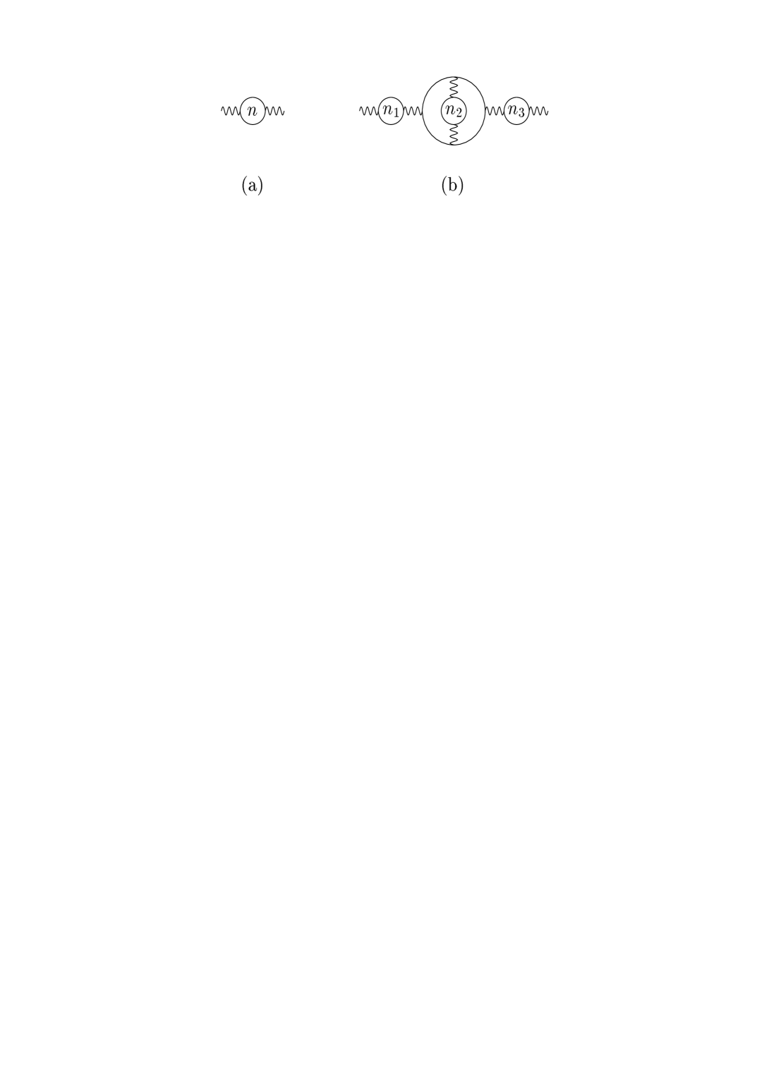
Figure 5: QED-like diagrams incorporating evolution of the coupling to leading (a) and next-to-leading order (b). A circle with letter $m$ denotes a chain of $m$ fermion loops. At order $\alpha^{k+1}$, the relevant diagrams are specified by $n=k$ and $n_{1}+n_{2}+n_{3}=k-2$. At NLO, the diagrams, where the $n_{2}$-chain forms a self-energy-type insertion, are not depicted.

$$R-R_{tree}=r_{0}\left[\alpha_{s}(Q^{*})+\delta_{1}\alpha_{s}(Q^{**})^{2}\ldots\right]\,.$$ (5.2)

Specifically, the scale of the coupling at order $\alpha_{s}$ is determined by the replacement

$$\alpha_{R}(Q)\rightarrow\alpha_{V}(k)\equiv\frac{\alpha_{R}(Q)}{1+\Pi_{R}(k^{2}/Q^{2},\alpha_{R}(Q))}$$ (5.3)

inside the loop-integration over $k$, where $k$ is the momentum of the virtual photon. We have attached a subscript $R$ to quantities that depend on the choice of the renormalization scheme $R$. On the right hand side we notice that $\alpha_{V}(Q)$ is the effective coupling, defined by the potential between two static sources in momentum space,

$$V(Q)=-\frac{4\pi\alpha_{V}(Q)}{Q^{2}}\,,$$ (5.4)

which defines the V-scheme [1]. Thus, in any scheme $R$, the scale $Q_{R}^{*}$ is given by averaging the lowest order radiative corrections to the quantity $R$ with the running coupling in the V-scheme, $\alpha_{V}(k)$, and not with $\alpha_{R}(k)$. By construction $\alpha_{R}(Q_{R}^{*})$ is scheme-independent. The choice of $\alpha_{V}(k)$ to average the loop momentum distribution is physically appropriate, because the photon exchanged between static sources at distance $r$ has momentum $k\sim 1/r$. Therefore it is in this scheme that $\alpha(k)$ can be interpreted as the effective coupling of a virtual photon of momentum $k$.

With this remark one is prepared to adopt the same definition in the nonabelian theory. $Q^{*}$ is defined as [5]

$$r_{0}\alpha_{R}(Q^{*})\equiv\int d^{4}k\,F(k,Q)\,\frac{\alpha_{V}(k)}{k^{2}}\,,$$ (5.5)

where $F(k,Q)$ is the integrand of the lowest order radiative correction and $C_{F}4\pi\alpha_{V}(k)/k^{2}$ the potential between two static colour sources in momentum space, given by a Wilson loop. The Wilson loop is nonperturbatively well-defined (up to a distance-independent contribution) and the above integral could be evaluated without any ambiguity. In the following, we will use it only perturbatively, in the sense of an expansion of $\alpha_{V}(k)$ in $\alpha_{V}(Q)$. This restriction is not only self-imposed. Power corrections to the static potential might be different and in particular larger than those to the quantity $R$, in which case one would not like to use Eq. (5.5) with power-like accuracy. Let us also note that one-loop gauge boson exchange exponentiates exactly in the abelian Wilson loop but not in the nonabelian case. Therefore re-expressing $\alpha_{V}(Q)$ in terms of some other $\alpha_{R}(Q)$ inevitably involves contributions to the Wilson loop with more than one gluon exchanged.

The exact (perturbative) evaluation of Eq. (5.5) is impossible even in the abelian theory. One has to resort to some truncation of (a) the $\beta$-function in the $V$-scheme, needed to relate $\alpha_{V}(k)$ to $\alpha_{V}(Q)$ and (b) the relation between the coupling in the V-scheme and some other scheme $R$, if one wishes to express the result in terms of $\alpha_{R}$. To leading order, the $\beta$-function has been replaced by $\beta_{0}\alpha^{2}$. After expansion of $\alpha(k)$ in $\alpha(Q)$, this corresponds to the diagrams of Fig. 5a in QED. In this section we discuss a truncation, which is guided by the subleading $N_{f}$-dependence of coefficients and incorporates the set of diagrams depicted in Fig. 5b in addition to those in Fig. 5a. Let us first consider $n_{1}=n_{3}=0$ in Fig. 5b. The diagram with $n_{2}=0$ gives $\beta_{1}\alpha^{3}$ to the abelian $\beta$-function. For $n_{2}>0$, these diagrams give contributions to higher order coefficients to the $\beta$-function. Again in QED, this contribution can be written as $b_{n_{2}+1}(-\beta_{1})(-\beta_{0})^{n_{2}}$ with a $N_{f}$-independent number $b_{n_{2}}$. When expanding $\alpha_{V}(k)$ as

$$\alpha_{V}(k)=\exp\left[\ln\frac{k^{2}}{Q^{2}}\,\beta_{V}(\alpha^{\prime})\frac{d}{d\alpha^{\prime}}\right]\alpha^{\prime}_{\big{|}\alpha^{\prime}=\alpha_{V}(Q)}\,,$$ (5.6)

the diagrams of Fig. 5 are recovered by using

$$\beta_{V}(\alpha)=\beta_{0}\alpha^{2}+\beta_{1}\sum_{n=1}^{\infty}b_{n}(-\beta_{0})^{n-1}\alpha^{n+2}\,,$$ (5.7)

but keeping only terms with at most one power of $\beta_{1}$. A different truncation could be imagined, where the $\beta$-function is kept only up to $\beta_{1}\alpha^{3}$ but all powers of $\beta_{1}$ are taken into account in the expansion of Eq. (5.6). The difference to the previous truncation appears first at order $\alpha^{5}$.

The transition to the nonabelian theory is arguably uniquely achieved at leading order by replacing the abelian $\beta_{0}$ by its nonabelian value. At NLO one has to make a choice which is less compulsory: Calculate the insertions of the diagrams of Fig. 5b and express them as $c_{n}(-\beta_{1})(-\beta_{0})^{n-2}\alpha(Q)^{n+1}$ in QED. Then replace $\beta_{0}$ and $\beta_{1}$ by their nonabelian values. In effect this implies substitution of the true $\beta$-function in the V-scheme by Eq. (5.7). We can now write the perturbative coefficients of the quantity $R$ as

$$r_{n}=r_{n0}+\ldots r_{nn-1}N_{f}^{n-1}+r_{nn}N_{f}^{n}\equiv r_{0}\left[\delta_{n}-\beta_{1}(-\beta_{0})^{n-2}c_{n}+(-\beta_{0})^{n}d_{n}\right]\qquad n\geq 2\,,$$ (5.8)

where, according to the prescription, the last two terms are absorbed into $Q^{*}$. Both sets of coefficients $c_{n}$ and $d_{n}$ are computed from abelian diagrams. Note that $d_{n}$ is constructed as to eliminate the highest power of $N_{f}$. On the other hand, to NLO, the remainder $\delta_{n}$ still contains subleading flavour dependence, $N_{f}^{n-1}$, which arises from insertion of fermion loops into diagrams with two gluon lines as well as the effective three-gluon coupling generated by attaching three gluons to a fermion loop.

Before turning to the calculation of $c_{n}$, we want to illustrate the prescription at order $\alpha_{s}^{3}$. Up to this order, the expansion of $R$ in a certain scheme with coupling $\alpha_{s}$ can be written as

$$R-R_{tree}=r_{0}\left[\alpha_{s}(Q)+\left\{\delta_{1}+(-\beta_{0})d_{1}\right\}\alpha_{s}(Q)^{2}+\left\{\delta_{2}-\beta_{1}c_{1}+(-\beta_{0})^{2}d_{2}\right\}\alpha_{s}(Q)^{3}\right]\,.$$ (5.9)

From Eq. (5.5) we obtain

$$\alpha_{s}(Q^{*})=\alpha_{V}(Q)+(-\beta_{0})d_{1}\alpha_{V}(Q)^{2}+\left\{(-\beta_{1})d_{1}+(-\beta_{0})^{2}d_{2}\right\}\alpha_{V}(Q)^{3}$$ (5.10)

where the (scheme-dependent) $d_{n}$ are computed as in Section 2 from diagrams with fermion loop insertions. By comparison we find that in the V-scheme ($\alpha_{s}(Q)=\alpha_{V}(Q)$) $c_{1}=d_{1}$. The remaining linear $N_{f}$-dependence in $\delta_{2}$ can then be absorbed into a scale $Q^{**}$ of the $\alpha_{s}^{2}$-correction [7]. Notice, however, that while $Q^{*}$ is defined without knowledge of the exact $\alpha_{s}^{3}$-coefficient, the definition of $Q^{**}$ in the nonabelian theory requires the exact $\alpha_{s}^{3}$-result.

To obtain the scale $Q^{*}$ as an expansion in the coupling different from the V-scheme, one has to relate the couplings to the same accuracy and expand $\alpha_{V}(Q)$ in, say, $\alpha_{\overline{\rm MS}}(Q)$ in the same form as Eq. (5.9):

$$\alpha_{V}(Q) = \alpha_{\overline{\rm MS}}(Q)+\left\{\gamma_{1}+(-\beta_{0})\left(-\frac{5}{3}\right)\right\}\alpha_{\overline{\rm MS}}(Q)^{2}$$ (5.11)

$$\,+\left\{\gamma_{2}-\beta_{1}\left(-\frac{55}{12}+4\zeta(3)\right)+(-\beta_{0})^{2}\frac{25}{9}\right\}\alpha_{\overline{\rm MS}}(Q)^{3}$$

One can then determine $c_{1}$ in the $\overline{\rm MS}$ scheme. Once $d_{1}$, $d_{2}$ and $c_{1}$ are determined, $Q^{*}_{2}$ to $\alpha_{s}^{3}$-accuracy is given by

$$Q^{*}_{2}=Q\,e^{-d_{1}/2}\left(1+\left\{(-\beta_{0})b_{1}+\tilde{b}_{1}\frac{\beta_{1}}{\beta_{0}}\right\}\alpha_{s}(Q)\right)\,.$$ (5.12)

$b_{1}$ and $\tilde{b}_{1}$ are uniquely determined by the condition

$$\alpha_{s}(Q^{*}_{2}) = \alpha_{s}(Q)+(-\beta_{0})d_{1}\alpha(Q)^{2}+\left\{(-\beta_{0})^{2}(d_{1}^{2}-2b_{1})-(d_{1}-2\tilde{b}_{1})\beta_{1}\right\}\alpha_{s}(Q)^{3}+\ldots$$ (5.13)

$$\equiv \alpha_{s}(Q)+(-\beta_{0})d_{1}\alpha(Q)^{2}+\left\{(-\beta_{0})^{2}d_{2}-\beta_{1}c_{1}\right\}\alpha_{s}(Q)^{3}\,,$$

which specifies that the diagrams of Fig. 5 relevant at order $\alpha_{s}^{3}$ are absorbed into $Q^{*}_{2}$ in any scheme. In the V-scheme $\tilde{b}_{1}=0$, but in general $\tilde{b}_{1}$ is non-zero.

In the V-scheme the prescription outlined here coincides exactly with the one by Brodsky and Lu [7]. When $Q^{*}_{2}$ is defined in other schemes, we suspect that $Q^{*}$ defined in [7] does not absorb the QED diagrams of Fig. 5b and part of the flavour-dependence from these diagrams is hidden in $Q^{**}$, since $\tilde{b}_{1}$ is always zero in [7].

When we compute $c_{n}$ in the following Section, rather than using the V-scheme in intermediate steps, we will perform the average of Eq. (5.5) directly in an arbitrary scheme by replacing $\alpha_{V}(k)$ with the appropriately truncated form of Eq. (5.3).

5.1 Abelian diagrams at NLO

We now evaluate the perturbative coefficients generated by inserting the chains of Fig. 5 into the gluon (photon) line which appears in lowest order radiative corrections to an observable $R$. In this subsection $\beta_{0}$ and $\beta_{1}$ refer to their abelian values: $\beta_{0}=N_{f}/(3\pi)$ and $\beta_{1}=N_{f}/(4\pi^{2})$. These chains have previously been considered for particular quantities: The muon anomalous magnetic moment [16] and the self-energy of a static quark [41]. Because vacuum polarization insertions are universal, the results can easily be adapted to the general case. The vacuum polarization to the present approximation is given by the diagrams with $n=1$ and $n_{1},n_{3}=0$ in Fig. 5 ($Q^{2}$ is euclidian):

$$\Pi\left(\frac{Q^{2}}{\mu^{2}},\alpha(\mu)\right)=-\beta_{0}\alpha(\mu)\left[\ln\frac{Q^{2}}{\mu^{2}}+C\right]+\beta_{1}\Pi_{1}\left(\frac{Q^{2}}{\mu^{2}},\alpha(\mu)\right)$$ (5.14)

When $\alpha_{V}(k)$ is expanded inside the integrand of Eq. (5.5), the result is expressed in terms of coefficients of the vacuum polarization and averages of $\ln^{n}(k^{2}/Q^{2})$ in the lowest order radiative correction $F(k,Q)$, which have already been evaluated through the insertion of the diagrams of Fig. 5a. Therefore, since $\Pi_{1}$ is known, the extension to incorporate Fig. 5b is merely a combinatorical problem. To organize the combinatorics, it is convenient to introduce the Borel transform. First, we define the leading order and next-to-leading order Borel transform as the result of insertion of diagrams with a single chain (Fig. 5a) and the sum of both diagrams in the Fig. 5. From Eq. (2.6) and Eq. (5.8):

$$B_{\rm LO}[R](u) \equiv r_{0}\sum_{n=0}^{\infty}\frac{d_{n}}{n!}u^{n}$$

$$B_{\rm NLO}[R](u) \equiv r_{0}\sum_{n=0}^{\infty}\frac{d_{n}^{\rm NLO}}{n!}u^{n}\qquad d_{n}^{\rm NLO}=d_{n}-\frac{\beta_{1}}{\beta_{0}^{2}}c_{n}\quad(n\geq 2)$$ (5.15)

and $d_{n}^{\rm NLO}=d_{n}$ for $n=0,1$. After Borel transformation of Eq. (5.5), the truncation of $\alpha_{V}(k)$ discussed above corresponds to insertion of

$$B\left[\frac{\alpha(Q)}{1+\Pi(k^{2}/Q^{2},\alpha(Q))}\right](u)=\left(\frac{k^{2}}{Q^{2}}e^{C}\right)^{-u}-\frac{\beta_{1}}{\beta_{0}^{2}}\int\limits_{0}^{u}dv\,v\left(\frac{k^{2}}{Q^{2}}e^{C}\right)^{-v}B\left[\frac{\Pi_{1}}{\alpha}\right](u-v)$$ (5.16)

into Eq. (5.5) instead of the complete $\alpha_{V}(k)$. On the right hand side, we have neglected multiple insertions of $\Pi_{1}$. The Borel transform of $\Pi_{1}/\alpha$ can be represented as

$$B\left[\frac{\Pi_{1}}{\alpha}\right](u)=\left(\frac{k^{2}}{Q^{2}}\right)^{-u}F(u)-G(u)\,,$$ (5.17)

where $F(u)$ is a scheme-independent function that can be obtained from Eq. (3.9) by integration with respect to $Q^{2}$:

$$F(u)=\frac{32}{3}\frac{1}{1-(1-u)^{2}}\sum_{k=2}^{\infty}\frac{(-1)^{k}k}{(k^{2}-(1-u)^{2})^{2}}\equiv\sum_{n=-1}^{\infty}f_{n}u^{n}$$ (5.18)

$G(u)$ is a scheme-dependent integration constant. One can use the renormalization group equation obeyed by the photon vacuum polarization to relate the expansion coefficients of $G(u)$ to those of the $\beta$-function in the chosen scheme. The precise relation is as follows: Let us write the highest power of $\beta_{n}$ as

$$\beta_{n\big{|}N_{f}^{n}}\equiv b_{n}\beta_{1}(-\beta_{0})^{n-1}\,.$$ (5.19)

Then

$$G(u)=\sum_{n=0}^{\infty}\frac{b_{n+1}}{n!}u^{n-1}\,,\qquad g_{n}=\frac{b_{n+2}}{(n+1)!}\,.$$ (5.20)

With these preliminaries, we insert Eq. (5.16) into Eq. (5.5) and obtain

$$B_{\rm NLO}[R](u) = B_{\rm LO}[R](u)-\frac{\beta_{1}}{\beta_{0}^{2}}\int\limits_{0}^{u}\frac{dv\,v}{u-v}\left(B_{\rm LO}[R](u)-B_{\rm LO}[R](v)\right)$$ (5.21)

$$\,-\frac{\beta_{1}}{\beta_{0}^{2}}\int\limits_{0}^{u}dv\,v\left(B_{\rm LO}[R](u)F_{\rm reg}(u-v)-B_{\rm LO}[R](v)G_{\rm reg}(u-v)\right)\,,$$

where $F_{\rm reg}(u)$ and $G_{\rm reg}(u)$ are defined by removing the pole at $u=0$: $F_{\rm reg}(u)\equiv F(u)-1/u$, $G_{\rm reg}(u)\equiv G(u)-1/u$.

The coefficients $d_{n}^{\rm NLO}$ are given by

$$d_{n}^{\rm NLO}=\frac{1}{r_{0}}\frac{d^{n}}{du^{n}}B_{\rm NLO}[R](u)_{|_{u=0}}\,.$$ (5.22)

Taking the derivatives of Eq. (5.21) we obtain (for $n\geq 2$)

$$d^{\rm NLO}_{n} = d_{n}-\frac{\beta_{1}}{\beta_{0}^{2}}n\,(\psi(n+1)-\psi(2))\,d_{n-1}$$ (5.25)

$$\,-\frac{\beta_{1}}{\beta_{0}^{2}}\sum_{k=0}^{n-2}\left[\left(\begin{array}[]{c}n\\ k\end{array}\right)f_{n-2-k}-(k+1)g_{n-2-k}\right](n-2-k)!\,d_{k}\,,$$

where $\psi(x)$ is the logarithmic derivative of the $\Gamma$-function. Note that for large $n$ the second term on the right side indeed dominates the first one by a factor $\beta_{1}/\beta_{0}^{2}\ln n$. With correspondingly changed conventions, this equation agrees with the corresponding one in [16]. The expansion coefficients of $F(u)$ are given by [16]

$$f_{n}=-\frac{2}{3}(n+2)\left[-2n-2-\frac{n+7}{2^{n+3}}+\frac{16}{n+2}\sum_{k=1}^{\left[\frac{n+3}{2}\right]}k(1-2^{-2k})(1-2^{2k-n-3})\zeta(2k+1)\right]\,,$$ (5.26)

where $\zeta(k)=\sum_{n=1}^{\infty}n^{-k}$ and $[..]$ denotes the integer part of the number in brackets. The coefficients $g_{n}$ depend on the scheme employed for the definition of $\alpha$. In the $\overline{\rm MS}$ scheme, we can use the $\beta$-function to the approximation required here from [39, 16]. We then find

$$g_{n}^{\overline{\rm MS}}=\frac{1}{(n+1)!(n+2)!}\frac{d^{n+1}}{du^{n+1}}\left[\frac{(1-u)(1+2u)(3+2u)\Gamma(4+2u)}{9\Gamma(2+u)^{2}\Gamma(3+u)\Gamma(1-u)}\right]_{\big{|}u=0}\,.$$ (5.27)

In the $V$-scheme, we have

$$g_{n}^{V}=f_{n}\,.$$ (5.28)

7,7,7 The simplest way to see this is that in this scheme by definition $\Pi(1,\alpha_{V}(Q))=0$. Then the expansion of the integrand in Eq. (5.5) has only non-zero powers of $\ln(k^{2}/Q^{2})$ and $d_{0}$ can not appear in Eq. (5.25).

5.2 Numerical analysis

The transition to QCD according to the prescription formulated above is performed by replacing $\beta_{1}/\beta_{0}^{2}$ in Eq. (5.25) by its QCD value. Note that contrary to $d_{n}$ the NLO coefficient depends explicitly on the number of flavours. In this Subsection, rather then presenting values for the BLM scale $Q^{*}$ to NLO accuracy, we give the perturbative coefficients in low orders generated by expansion of of $\alpha_{s}(Q^{*})$ in the $\overline{\rm MS}$-coupling, that is the coefficients $d_{n}^{\rm NLO}$ and $M^{\rm NLO}_{n}(-\beta_{0}\alpha_{s})$, defined in complete analogy with $M_{n}(-\beta_{0}\alpha_{s})$. To compare the coefficients obtained from keeping only vacuum polarization with the exact ones, if available, we shall also define $d_{n}^{\rm exact}$ as the exact coefficient, divided by $(-\beta_{0})^{n}$. Numerical values for the difference between pole and $\overline{\rm MS}$ mass are shown in Table 7, and for the derivative of the hadronic vacuum polarization $Q^{2}d\Pi/dQ^{2}$ and the $\tau$ decay width in Tables 7 and 7.

$$\begin{array}[]{|c||c|c|c|c|}\hline\cr n&d_{n}&d_{n}^{\rm NLO}&M_{n}\,[\mbox{b-quark}]&M_{n}^{\rm NLO}\,[\mbox{b-quark}]\\ \hline\cr\hline\cr 0&1&1&1&1\\ 1&4.68615&4.68615&1.623&1.623\\ 2&17.6227&19.6884&1.935&1.972\\ 3&109.859&127.529&2.193&2.272\\ 4&873.924&1138.28&2.467&2.628\\ 5&8839.69&12085.6&2.835&3.131\\ \hline\cr\end{array}$$

Table 5: Comparison of leading order and next-to-leading order coefficients for the difference of pole and $\overline{\rm MS}$ mass, where quark masses inside loops are neglected and loops containing the heavy quark are excluded (cf. Sect. 4). The comparison of the modification of lowest order radiative corrections is for $\alpha_{s}(m_{b})=0.2$, relevant to bottom quarks.

$$\begin{array}[]{|c||c|c|c||c|c|c|}\hline\cr n&d_{n}&d^{\rm NLO}_{n}&d_{n}^{\rm exact}&M_{n}&M^{\rm NLO}_{n}&M^{\rm exact}_{n}\\ \hline\cr\hline\cr 0&1&1&1&1&1&1\\ 1&0.691772&0.691772&0.728809&1.158&1.158&1.167\\ 2&3.10345&2.31417&1.25847&1.321&1.271&1.233\\ 3&2.18004&7.40378&-&1.347&1.360&-\\ 4&30.7398&18.4580&-&1.432&1.411&-\\ 5&-34.5336&146.293&-&1.410&1.503&-\\ \hline\cr\end{array}$$

Table 6: Comparison of leading order, next-to-leading order and exact coefficients of $Q^{2}d\Pi(Q)/dQ^{2}$. The NLO and exact values are given for $N_{f}=3$ and the partial sums $M_{n}$ for $\alpha_{s}=0.32$. Exact values, when available, include genuine higher order corrections.

$$\begin{array}[]{|c||c|c|c||c|c|c|}\hline\cr n&d_{n}&d^{\rm NLO}_{n}&d_{n}^{\rm exact}&M_{n}&M^{\rm NLO}_{n}&M^{\rm exact}_{n}\\ \hline\cr\hline\cr 0&1&1&1&1&1&1\\ 1&2.27511&2.27511&2.31213&1.521&1.521&1.529\\ 2&5.68475&5.98780&5.20806&1.819&1.835&1.803\\ 3&13.7536&18.1248&-&1.984&2.053&-\\ 4&35.1470&54.7939&-&2.081&2.203&-\\ 5&84.4066&178.897&-&2.134&2.316&-\\ \hline\cr\end{array}$$

Table 7: Same as in the previous table for the perturbative expansion of the $\tau$ hadronic width ($\alpha_{s}(m_{\tau})=0.32$).

The main conclusion for the radiative mass shift is that the effect of two-loop running remains small up to the order, at which the series has to be truncated. It leads to a less then 5% additional increase of the one-loop radiative correction, which can be neglected in view of the uncertainties that have been discussed in Sect. 4. This is reassuring, because it supports the suggestion that the mass shift is to a large extent given by one-loop running effects, although it must be borne in mind that by incorporating two-loop running one does not gain control over genuine two- and higher loop corrections.

On the other hand, the effect of two-loop running is very large for the derivative of the vacuum polarization and the efficiency of extending the BLM prescription beyond leading order can be doubted in this case. Although the inclusion of two-loop running improves the estimate of $d_{2}$ as compared to the exact coefficient $d_{2}$ (Table 7), for $n>3$ the effect of two-loop running is exceedingly large and this improvement might as well be accidental.

It is interesting to observe that for the $\tau$ hadronic width itself (Table 7), such irregularities do not occur, which is in qualitative agreement with the conclusion of Sect. 3.1 that the perturbative expansion of $R_{\tau}$ has a smoother behaviour in intermediate orders of perturbation theory than $Q^{2}d\Pi/dQ^{2}$. The relative importance of two-loop running increases with $n$ as expected from the asymptotic $\ln n$-enhancement. Though smooth, the effect of two-loop running is significant for $R_{\tau}$ and points towards an even further increase of the cumulative effect of higher order perturbative corrections and consequently a further decrease of $\alpha_{s}(m_{\tau})$ from $R_{\tau}$.

In Appendix C, we give exact results for the five-loop diagrams that enter the calculation of $d_{3}^{\rm NLO}$ for $Q^{2}d\Pi/dQ^{2}$.

6 Conclusions

In this paper we have shown how to deal with higher order vacuum polarization insertions into radiative corrections to observables in QCD. This enterprise has been motivated by the fact that these higher order corrections often lead to disturbingly large coefficients in the perturbative expansion. This trend is systematic, but since it can be identified, we suggest to calculate these corrections and separate them from the remaining ones. The behaviour of the remaining series should then be improved. Even if the remaining corrections turn out not to be small, the summation of vacuum polarization insertions can be motivated as a physical way of scale-setting. In this respect it can be considered as an extension of the scale-setting proposed by Brodsky, Lepage and Mackenzie [1] and Brodsky and Lu [7], as far as two-loop running is concerned. It is worth noting that the familiar BLM scale typically overestimates the size of higher order vacuum polarization insertions. The smallness of this scale needs not necessarily indicate a failure of perturbation theory, unless it is indicative of its divergence already at two-loop order.

We would like to stress the computational ease with which the summation of effects of one-loop running can be performed compared to a genuine higher order calculation. We thus have devoted considerable space to technical aspects, which should allow routine implementation of this summation. The two existing techniques can be summarized as follows: The first one [14, 16, 17, 3] amounts to direct evaluation of the relevant higher order Feynman diagrams. A convenient tool to organize such a calculation is the Borel transform. The result can be obtained as a certain analytically regularized Feynman integral plus – if necessary – a subtraction function that is easily computed directly from a large-mass expansion. This technique has its limits, when applied to processes with several scales or to physical cross sections that are more directly calculated as a sum of real and virtual corrections. In these cases, we have applied a dispersion technique [20, 12, 4] (or, if one starts from the Borel transform, a Mellin transformation) to reduce the problem to calculation of lowest order corrections with finite gluon mass. It is in this representation, that summation (up to an accuracy set by renormalons) is most easily performed. This summation is usually complicated by the need to analytically continue the Borel transform beyond its radius of convergence and to take the (principal value) integral over the Borel parameter. Our Eqs. (2.24) and (2.29) are immediately suited to numerical evaluation. Given this simplicity, the computational expense seems worth the investment even if one could only hope to absorb a higher order radiative correction that has the correct sign compared to the exact one.

In the present paper, we have investigated two quantities in more detail. Higher order $\beta_{0}^{n}\alpha_{s}^{n+1}$-corrections are indeed sizeable for the hadronic decay width of the $\tau$ lepton, when expressed as a series in $\alpha_{s}$. We compared fixed order perturbative approximations to $R_{\tau}$ with those from a partial resummation of running coupling effects due to contour integration [10] and found that in intermediate orders the first one has a smoother behaviour, since potentially large corrections from contour integration conspire with the divergent coefficients of $Q^{2}d\Pi/dQ^{2}$ to produce an effective suppression of ultraviolet renormalons (Table 1). Resummation of all one-loop running coupling effects leads to an approximate 10% decrease of $\alpha_{s}(m_{\tau})$ determined from hadronic $\tau$ decays to a central value of

$$\alpha_{s}(m_{\tau})\simeq 0.29\,.$$ (6.1)

This shift of about one error margin of previous analyses is not caused by a single large next-order coefficient, but by the constructive addition of several higher order coefficients beyond the exactly known coefficient at order $\alpha_{s}^{3}$.

The accurate extraction of $\alpha_{s}$ from $\tau$-decays relies on the absence of $\Lambda_{\rm QCD}^{2}/m_{\tau}^{2}$-corrections. Although from a purely theoretical point of view, the situation with respect to such terms is not conclusive, given that the limitations of duality are only poorly understood, we conclude that effects associated with summation of the divergent perturbative expansion should be excluded as a source of such terms, provided one accepts their absence in the relevant current correlation functions in euclidian space.

For the difference between the pole and $\overline{\rm MS}$-renormalized mass of a heavy quark, we conclude that the large two-loop correction found in [38] is probably not accidental but the first one in a rapidly divergent series of higher order corrections dominated indeed by one-loop running of the coupling. For the charm quark, the divergence is such that the perturbative series can certainly not be improved beyond two-loop order. For the bottom pole mass, our estimate incorporating one-loop running reads

$$\frac{\delta M_{b}}{M_{b}}=(16.3\pm 2.9\pm 1.5)\%\,,$$ (6.2)

which is about 30% larger than the two-loop result without resummation. We expect this difference to be significant in phenomenological applications. The first error quoted is associated with the divergence of the series that relates the two mass definitons and is irreducible. Numerically this error amounts to an uncertainty somewhat larger than 100 MeV for the mass difference, a value in between the estimates initially reported in [37, 17]. Short-distance observables containing quark masses, when expressed in terms of pole masses will generally exhibit large coefficients implanted by the use of this parameter. Thus, although both mass definitions are ultimately unphysical, we expect that the $\overline{\rm MS}$ mass can be determined to better accuracy through perturbative relations.

Finally, let us mention that the calculation of vacuum polarization can never replace an exact calculation. Until this is completed, we find it worthwhile to incorporate the systematic effects exhibited by one-loop running. Surely, the authors are among those who await further exact results with suspense.

Note added. While this paper was written, we were informed by M. Neubert on work of his, which partially overlaps with the present one. We acknowledge exchange of manuscripts and are very grateful for the ensuing discussions which helped to clarify our presentation. We disagree with the conclusion of [42] that the difference of various summation prescriptions for cross sections should be interpreted as a sign and quantification of the failure of the operator product expansion in the physical region. As emphasized in Sect. 3.2, once one abandones Borel-summation type prescriptions, which are distinguished by their relation to the OPE, one can introduce $1/Q^{2}$-differences in euclidian space just as well and there is no discrimination between the euclidian and minkowskian region from the point of view of summation of perturbation theory, given the present state of knowledge.

Acknowledgements. M. B. would like to thank D. Broadhurst and A. Pich for stimulating discussions. M. B. is supported by the Alexander von Humboldt-foundation.

Appendices

Appendix A Subtractions

In general, we will also be interested in ultraviolet divergent quantities. Examples include the difference between the pole mass and the $\overline{\rm MS}$-renormalized quark mass and the correlation function of heavy-light currents in heavy quark effective theory. Denoting a generic quantity by $R(\alpha)$, the renormalized Borel transform has the form

$$B[R](u)=B[R]_{0}(u)+S_{R}(u)\,,$$ (A.1)

where $B[R]_{0}(u)$ is the bare Borel transform, calculated from diagrams without overall subtraction, using the Borel parameter itself as a regulator. This corresponds to analytic regularization [15]. Consequently, the bare Borel transform is singular at the origin (Recall that the perturbative series is generated by derivatives of the Borel transform at the origin.). This singularity is subtracted by the function $S_{R}(u)$, which depends on the renormalization scheme. In minimal subtraction schemes $uS_{R}(u)$ is an entire function (at least for one chain of fermion loops) and – when combined with the appropriate singular piece of $B[R]_{0}(u)$ to be defined below, Eq. (A.1) – $S_{R}(u)$ yields an unambiguous contribution to the bubble sum

$$S_{R}(\alpha)\equiv\left(-\frac{1}{\beta_{0}}\right)\int\limits_{0}^{\infty}du\,e^{-u/(-\beta_{0}\alpha)}\,\Big{(}S_{R}(u)+\mbox{singular term in }B[R]_{0}(u)\Big{)}\,.$$ (A.2)

General expressions for $S_{R}(u)$ in minimal subtraction schemes have been derived in Appendix A of [17]. In this Appendix we outline a simple method to obtain $S_{R}(u)$ and calculate $S_{R}(\alpha)$ in minimal subtraction schemes. An essential simplification comes from the fact that one needs only the dominant large-$\lambda$ behaviour of dimensionally regularized Feynman amplitudes, where $\lambda$ is a mass for the gluon. As an illustration of the technique we calculate the subtractions for the correlation function of two heavy-light currents in heavy quark effective theory.

A.1 Calculation of $S_{R}(\alpha)$

As always we assume that the quantity $R$ has been made dimensionless, is infrared finite and such that the order-$\alpha$ radiative correction comes from gluon exchange. We shall also assume that the corresponding diagrams have one loop and are at most logarithmically ultraviolet divergent. The last assumption is actually unnecessary, see the explicit example in the subsequent subsection. The dimensionally regularized order-$\alpha$ correction can then be represented as

$$r_{0}^{\rm bare}(\epsilon)\,\alpha=\alpha\mu^{2\epsilon}\int d^{d}k\,F(k,Q)\frac{1}{k^{2}}\,.$$ (A.3)

We use $d=4-2\epsilon$ and denote by $Q$ a set of external momenta. For gauge-dependent quantities, we take Landau gauge. The factor $(k_{\mu}k_{\nu}/k^{2}-g_{\mu\nu})$ from the gluon propagator is included in the integrand $F(k,Q)$ and we do not write Lorentz indices explicitly. We define the both, dimensionally and analytically regularized coefficient by

$$\hat{r}_{0}^{\rm bare}(s,\epsilon)\alpha=\alpha\mu^{2\epsilon}\int d^{d}k\,F(k,Q)\frac{1}{k^{2}}\left(-\frac{\mu^{2}}{k^{2}}\right)^{s}\,,$$ (A.4)

where $\mu$ is a subtraction scale. Note that $B[R]_{0}(u)=\hat{r}_{0}^{\rm bare}(u,\epsilon=0)\,e^{-uC}$, see Eq. (2.12).

Insert $n$ fermion loops into the gluon line of all diagrams that generate $r_{0}$. The fermion loop integrations can be done. Each loop gives a factor

$$-\frac{\beta_{0}^{f}}{\epsilon}\frac{6\Gamma(1+\epsilon)\Gamma(2-\epsilon)^{2}}{\Gamma(4-2\epsilon)}\left(-\frac{k^{2}}{4\pi\mu^{2}}\right)^{-\epsilon}\,,$$

where $\beta_{0}^{f}=T/(3\pi)$ is the fermionic contribution to the beta-function ($T=1$ in QED and $T=1/2$ in QCD). Performing the final integration over gluon momentum $k$, the result for the coefficient of order $\alpha^{n+1}$ can be written as

$$r_{n}^{\rm bare}(\epsilon)=\frac{\left(\beta_{0}^{f}\right)^{n}}{(n+1)(-\epsilon)^{n+1}}\,G(-\epsilon,-(n+1)\epsilon)$$ (A.5)

$$G(-\epsilon,-(n+1)\epsilon)=\left((4\pi)^{\epsilon}\frac{6\Gamma(1+\epsilon)\Gamma(2-\epsilon)^{2}}{\Gamma(4-2\epsilon)}\right)^{n}(n+1)(-\epsilon)\,\hat{r}_{0}^{\rm bare}(s=n\epsilon,\epsilon)\,,$$ (A.6)

where Eq. (A.4) has been used. The function $G$ introduced above coincides with the one of Appendix A of [17] [Note that $d=4+2\epsilon$ has been used in [17], which motivates the signs in the arguments of $G$ above.]. To obtain the subtraction function $S_{R}(u)$ in the $\overline{\rm MS}$ scheme, one has to add to $r_{n}^{\rm bare}(\epsilon)$ the diagrams with fermion loops replaced by their $\overline{\rm MS}$ counterterms and then compute the finite part of the sum. For any quantity $R$, the steps of Appendix A in [17] for the self-energy of a heavy quark can be repeated with the general result

$$S_{R}(u)=\frac{\tilde{G}_{0}(u)}{u}\qquad\tilde{G}_{0}(u)=\sum_{n=0}^{\infty}\frac{g_{n}}{n!}u^{n}\,,$$ (A.7)

where $g_{n}$ are the expansion coefficients of

$$G_{0}(-\epsilon)\equiv G(-\epsilon,-(n+1)\epsilon=0)=\sum_{m=0}^{\infty}g_{m}(-\epsilon)^{m}\,.$$ (A.8)

Since $G_{0}$ is related to subtractions, it should be unnecessary to calculate the full diagram, encoded in the function $G$, in order to obtain $G_{0}$. We prove that $G_{0}$ can be deduced from the large-mass expansion of the dimensionally regularized one-loop coefficient $r_{0}^{\rm bare}(\lambda^{2},\epsilon)$ computed with a gluon mass $\lambda$. That is, $1/k^{2}$ in Eq. (A.3) is replaced by $1/(k^{2}-\lambda^{2})$ (in Landau or Feynman gauge). Since the original four-dimensional integral was logarithmically ultraviolet divergent, the asymptotic behaviour at large $\lambda$ is given by

$$r_{0}^{\rm bare}(\lambda^{2},\epsilon)\stackrel{{\scriptstyle\lambda^{2}\rightarrow\infty}}{{=}}-\frac{1}{\epsilon}\,r_{\infty}(\epsilon)\left(\frac{\mu^{2}}{\lambda^{2}}\right)^{\epsilon}\,.$$ (A.9)

This equation defines the $\lambda^{2}$-independent function $r_{\infty}(\epsilon)$. Its value at $\epsilon=0$ is denoted by $r_{\infty}$. By definition

$$G_{0}(-\epsilon)=-\frac{1}{(4\pi)^{\epsilon}}\frac{\Gamma(4-2\epsilon)}{6\Gamma(1+\epsilon)\Gamma(2-\epsilon)^{2}}\,\lim_{s\rightarrow-\epsilon}\,(s+\epsilon)\,\hat{r}_{0}^{\rm bare}(s,\epsilon)\,.$$ (A.10)

To evaluate the limit, we use that $\hat{r}_{0}^{\rm bare}(s,\epsilon)$ is related to the one-loop coefficient with finite gluon mass $r_{0}^{\rm bare}(\lambda^{2},\epsilon)$ by a Mellin transform:

$$\hat{r}_{0}^{\rm bare}(s,\epsilon)=-\frac{\sin\pi s}{\pi}\int\limits_{0}^{\infty}\frac{d\lambda^{2}}{\lambda^{2}}\left(\frac{\lambda^{2}}{\mu^{2}}\right)^{-s}r_{0}^{\rm bare}(\lambda^{2},\epsilon)$$ (A.11)

This represents the analytic continuation of the analogon of Eq. (2.17) into the $u$-interval $]-\epsilon,0[$. Integrating by parts, we get

$$\hat{r}_{0}^{\rm bare}(s,\epsilon)=-\frac{\sin\pi s}{\pi\,(s+\epsilon)}\int\limits_{0}^{\infty}d\lambda^{2}\left(\frac{\lambda^{2}}{\mu^{2}}\right)^{-(s+\epsilon)}\!f^{\prime}(\lambda^{2},\epsilon)\,,$$ (A.12)

where $f(\lambda^{2},\epsilon)$ is defined by dividing $\hat{r}_{0}^{\rm bare}(s,\epsilon)$ by $(\mu^{2}/\lambda^{2})^{\epsilon}$. The limit is now easily taken with the result

$$\lim_{s\rightarrow-\epsilon}\,(s+\epsilon)\,\hat{r}_{0}^{\rm bare}(s,\epsilon)=-\frac{\sin\pi\epsilon}{\pi\epsilon}\,r_{\infty}(\epsilon)\,.$$ (A.13)

This yields the final result

$$G_{0}(u)=\frac{1}{(4\pi)^{-u}}\frac{\Gamma(4+2u)}{6\Gamma(1-u)\Gamma(2+u)^{2}}\,\frac{\sin\pi u}{\pi u}\,r_{\infty}(-u)\,.$$ (A.14)

The computation of the subtraction function has been reduced to calculation of the large mass limit of one-loop corrections with non-zero gluon mass.

Combining Eq. (2.17) for the bare Borel transform with Eq. (A.7), the renormalized Borel transform is given by

$$B[R](u)=-\frac{\sin\pi u}{\pi u}\int\limits_{0}^{\infty}d\lambda^{2}\left(\frac{\lambda^{2}}{\mu^{2}}e^{C}\right)^{-u}r_{0}^{\prime}(\lambda^{2})+\frac{\tilde{G}_{0}(u)}{u}\,.$$ (A.15)

The derivative $r_{0}^{\prime}(\lambda^{2})$ is ultraviolet finite, which allows to put $\epsilon=0$. However, the integral is not yet finite at $u=0$ and the above expression is not suited to take derivatives at $u=0$. Since, by Eq. (A.9), $r_{0}^{\prime}(\lambda^{2})=r_{\infty}/\lambda^{2}$ for large $\lambda^{2}$, we obtain

$$B[R](u) = -\frac{\sin\pi u}{\pi u}\int\limits_{0}^{\infty}d\lambda^{2}\left(\frac{\lambda^{2}}{\mu^{2}}e^{C}\right)^{-u}\left[r_{0}^{\prime}(\lambda^{2})-\frac{r_{\infty}}{\lambda^{2}}\,\Theta(\lambda^{2}-\mu^{2}e^{-C})\right]$$ (A.16)

$$\,+\frac{1}{u}\left(\tilde{G}_{0}(u)-r_{\infty}\,\frac{\sin\pi u}{\pi u}\right)\,.$$

In this form the integral exists for $u=0$ and the second line is finite at $u=0$. We note that this expression is equivalent to, but slightly different from the one given in [4]. In the present form $\mu^{2}$ and $C$ appear only in their natural combination $\mu^{2}e^{-C}$.

To obtain the bubble sum, all steps that lead from Eq. (2.17) to Eq. (2.24) can now be repeated on the first line of Eq. (A.16). The Borel integral of the second line is given by

$$S_{R}(\alpha) \equiv \left(-\frac{1}{\beta_{0}}\right)\int\limits_{0}^{\infty}du\,e^{-u/(-\beta_{0}\alpha)}\,\frac{1}{u}\left(\tilde{G}_{0}(u)-r_{\infty}\,\frac{\sin\pi u}{\pi u}\,e^{-uC}\right)$$

$$= \left(-\frac{1}{\beta_{0}}\right)\int\limits_{0}^{-\beta_{0}\alpha}\frac{du}{u}\left(G_{0}(u)-r_{\infty}\right)-\frac{r_{\infty}}{\beta_{0}}\left[\frac{\arctan(\pi\beta_{0}\alpha)}{\pi\beta_{0}\alpha}+\frac{1}{2}\ln\left(1+\pi^{2}\beta_{0}^{2}\alpha^{2}\right)-1\right]\,.$$

Thus, in case subtractions are required beyond coupling renormalization, Eq. (2.24) is replaced by

$$r_{0}a_{s}M_{\infty}(a_{s}) = \int_{0}^{\infty}d\lambda^{2}\,\Phi(\lambda^{2})\,\left(r^{\prime}_{0}(\lambda^{2})-\frac{r_{\infty}}{\lambda^{2}}\,\Theta(\lambda^{2}-\mu^{2}e^{-C})\right)+[r_{0}(\lambda_{L}^{2})-r_{0}(0)]$$ (A.18)

$$\,+\int\limits_{0}^{\,a_{s}}\frac{du}{u}\left(G_{0}(u)-r_{\infty}\right)+r_{\infty}\left[\frac{\arctan(\pi a_{s})}{\pi a_{s}}+\frac{1}{2}\ln\left(1+\pi^{2}a_{s}^{2}\right)-1\right]\,,$$

with $G_{0}(u)$ given by Eq. (A.14).

A.2 A sample calculation

As a non-trivial example, we calculate the subtraction function for the correlation function of heavy-light currents in heavy quark effective theory,

$$\Pi_{5}(\omega)\,=\,i\int{\mbox{d}}^{4}x\,e^{i\omega(v\cdot x)}\,\langle 0|T\{j_{5}^{\dagger}(x)j_{5}(0)\}|0\rangle\qquad j_{5}(x)=\bar{h}_{v}(x)i\gamma_{5}q(x)\,.$$ (A.19)

The corresponding bare Borel transform has been given in [17]. At first sight the method exposed in the previous subsection appears inapplicable, because the diagrams to be considered have two loops, see Fig. 6, and, because the correlation function is quadratically divergent, one also needs subtractions for the two-loop diagram itself. To eliminate these, we shall consider the third derivative

$$D(\omega)\equiv\omega\,\frac{{\mbox{d}}^{3}\Pi_{5}(\omega)}{{\mbox{d}}\omega^{3}}\,.$$ (A.20)

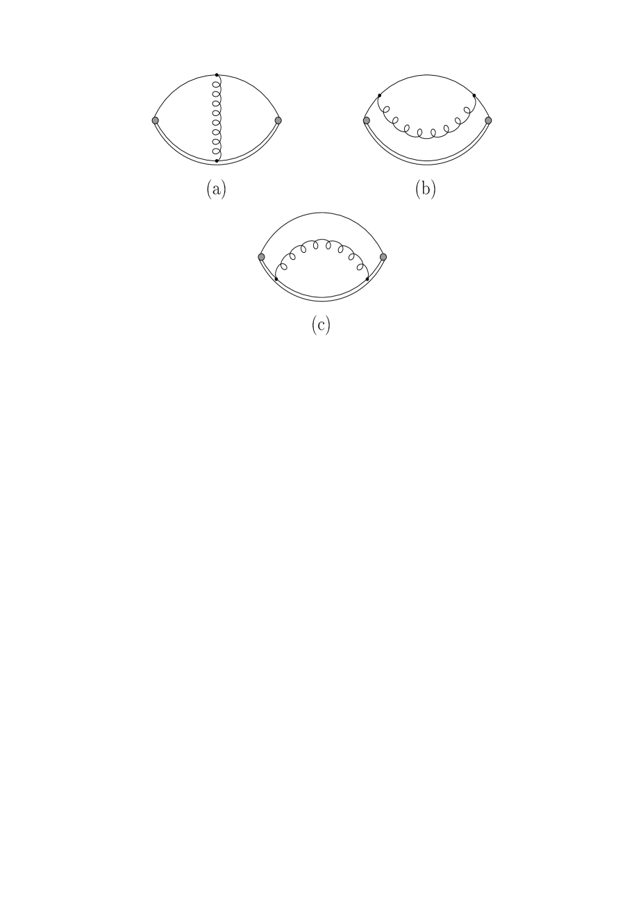
Figure 6: Radiative corrections to the correlation function of heavy-light currents. The shaded circle represents a current insertion with momentum $q$ and the double line denotes a heavy quark propagator.

Then all subtractions originate from divergent one-loop subdiagrams, which are subsequently inserted in the lowest order one-loop diagram for $\Pi_{5}(\omega)$. We remind the reader that the heavy-light current in the effective theory is not conserved. We treat the three diagrams in turn and take Landau gauge.

Let us start with diagram (a) and investigate the one-loop correction to the heavy-light vertex with non-zero gluon mass. The numerator of the corresponding Feynman integrand is proportional to

$$\gamma^{\rho}(\!\not\!q-\!\not\!k)\gamma_{5}v^{\tau}(k^{2}g_{\rho\tau}-k_{\rho}k_{\tau})\,,$$ (A.21)

where $v$ is the velocity of the heavy quark and the momentum assignments to the lines of the diagram are evident. Since the contribution proportional to $\lambda^{-2\epsilon}$ required by Eq. (A.9) comes from $k\sim\lambda\gg q$, we can drop $\not\!\!q$ in the above expression and the integral is simplified to

$$\int\frac{d^{d}k}{(2\pi)^{d}}\frac{\!\not\!v\!\not\!k-v\cdot k}{(q-k)^{2}\,v\cdot(q^{\prime}-k)\,(k^{2}-\lambda^{2})}\,.$$ (A.22)

The corresponding integral with numerator replaced by $k_{\mu}$ has structure $F_{1}v_{\mu}+F_{2}q_{\mu}+F_{3}q_{\mu}^{\prime}$. By dimensional counting, only $F_{1}$ can behave as $\lambda^{-2\epsilon}$ for large $\lambda^{2}$, the other structures being suppressed by powers of $\lambda$. But then the potential term $\lambda^{-2\epsilon}$ is proportional to $\!\not\!v\!\not\!v-v^{2}=0$ and therefore $r_{\infty}(\epsilon)$ vanishes identically for this diagram (This property is specific to Landau gauge.).

For diagram (b) we need the self-energy insertion of a light (massless) quark, given by

$$-C_{F}g^{2}\mu^{2\epsilon}\int\frac{d^{d}k}{(2\pi)^{d}}\frac{\gamma^{\rho}(\!\not\!p-\!\not\!k)\gamma^{\tau}}{(p-k)^{2}(k^{2}-\lambda^{2})}\,\left[g_{\rho\tau}-\frac{k_{\rho}k_{\tau}}{k^{2}}\right]\,,$$ (A.23)

where $p$ is the external momentum for the subdiagram. Again the term involving $\lambda^{-2\epsilon}$ in the large $\lambda^{2}$-expansion comes from $k\sim\lambda\gg p$, which allows to expand the propagator $1/(p-k)^{2}$. The integrand simplifies to

$$\frac{\gamma^{\rho}(\!\not\!p-\!\not\!k)\gamma^{\tau}}{(p-k)^{2}(k^{2}-\lambda^{2})}\,\left[g_{\rho\tau}-\frac{k_{\rho}k_{\tau}}{k^{2}}\right]\longrightarrow\frac{\epsilon\,(3-2\epsilon)}{2-\epsilon}\frac{\!\not\!p}{k^{2}(k^{2}-\lambda^{2})}+O\left(\frac{1}{k^{5}}\right)\,,$$ (A.24)

where the neglected terms do not produce a $\lambda^{-2\epsilon}$ contribution. The result is

$$(-i)\!\not\!p\left(\frac{4\pi\mu^{2}}{\lambda^{2}}\right)^{\epsilon}\frac{C_{F}\alpha}{4\pi}\frac{(3-2\epsilon)\Gamma(1+\epsilon)}{(1-\epsilon)(2-\epsilon)}\,.$$ (A.25)

Integration of the final quark loop is straightforward, and taking three subtractions we obtain

$$G_{0}^{(b)}(u)=\frac{C_{F}N_{c}}{4\pi^{3}}\left[-\frac{u}{6}(3+2u)\frac{\Gamma(4+2u)}{\Gamma(1-u)\Gamma(2+u)^{2}\Gamma(3+u)}\right]\,.$$ (A.26)

Turning to the self-energy of a heavy quark in heavy quark effective theory in diagram (c), we encounter another apparent obstacle to applying the technique of the previous subsection: The subdiagram is linearly ultraviolet divergent, and – at large $\lambda^{2}$ – behaves like $\lambda^{1-2\epsilon}$. The remedy is simply to ignore this term and pick up the term $\lambda^{-2\epsilon}$, since power divergences are discarded in minimal subtraction schemes. The large mass expansion of the heavy quark self-energy is

$$(-i)\frac{1+\!\not\!v}{2}\left(\frac{4\pi\mu^{2}}{\lambda^{2}}\right)^{\epsilon}\frac{C_{F}\alpha}{4\pi}\left[\Gamma\left(\frac{1}{2}\right)\Gamma\left(\epsilon-\frac{1}{2}\right)\,\lambda+\frac{(3-2\epsilon)\Gamma(\epsilon)}{1-\epsilon}\,v\cdot p+O\left(\frac{v\cdot p}{\lambda}\right)\right]\,.$$ (A.27)

Discarding the first term and inserting the remaining one into the quark loop, we get

$$G_{0}^{(c)}(u)=\frac{C_{F}N_{c}}{4\pi^{3}}\left[\frac{1}{6}(3+2u)\frac{\Gamma(4+2u)}{\Gamma(1-u)\Gamma(2+u)^{3}}\right]\,.$$ (A.28)

Adding the contributions from all diagrams, the result is

$$G_{0}(u)=\frac{C_{F}N_{c}}{4\pi^{3}}\left[\frac{1}{3}(3+2u)\frac{\Gamma(4+2u)}{\Gamma(1-u)\Gamma(2+u)^{2}\Gamma(3+u)}\right]\,.$$ (A.29)

Appendix B Radiative corections to $R_{e^{+}e^{-}}$ and $R_{\tau}$ with finite gluon mass

We write the lowest order radiative corrections to the total cross section of $e^{+}e^{-}$ annihilation and the hadronic $\tau$ decay width with finite gluon mass $\lambda$ as

$$R_{e^{+}e^{-}} = 3\left[1+\alpha_{s}(s)\left\{r_{e^{+}e^{-}}^{virt}(y)+\Theta(1-y)\,r_{e^{+}e^{-}}^{real}(y)\right\}\right]\,,$$ (B.1)

$$R_{\tau} = 3\left[1+\alpha_{s}(m_{\tau})\left\{r_{\tau}^{virt}(y)+\Theta(1-y)\,r_{\tau}^{real}(y)\right\}\right]\,,$$ (B.2)

where $y=\lambda^{2}/s$ or $y=\lambda^{2}/m_{\tau}^{2}$, respectively. Quarks are taken as massless. $r^{virt}(y)$ are virtual and $r^{real}(y)$ real gluon emission corrections:

$$r_{e^{+}e^{-}}^{virt}(y) = \frac{2}{3\pi}\Bigg{[}2(1+y)^{2}\Bigg{\{}-\frac{1}{2}\ln^{2}y+\ln y\ln(1+y)+\frac{\pi^{2}}{6}+\mbox{Li}_{2}(-y)\Bigg{\}}$$ (B.3)

$${}-\frac{7}{2}-2y-3\ln y-2y\ln y\Bigg{]}$$

$$r_{e^{+}e^{-}}^{real}(y) = \frac{2}{3\pi}\Bigg{[}2(1+y)^{2}\Bigg{\{}\frac{1}{2}\ln^{2}y-2\ln y\ln(1+y)-\frac{\pi^{2}}{6}-2\mbox{Li}_{2}(-y)\Bigg{\}}$$ (B.4)

$${}+5-5y^{2}+3\ln y+4y\ln y+3y^{2}\ln y\Bigg{]}\,,$$

and

$$r_{\tau}^{virt}(y) = \frac{1}{324\pi}\Bigg{[}-2577+72\pi^{2}+(2392-240\pi^{2})\,y+(828-432\pi^{2})\,y^{2}+144(1-\pi^{2})\,y^{3}$$ (B.5)

$$-24\pi^{2}y^{4}-1332\ln y+(2208+288\pi^{2})\,y\ln y+792y^{2}\ln y+144y^{3}\ln y-216\ln^{2}y$$

$$+720y\ln^{2}y+1296y^{2}\ln^{2}y+432y^{3}\ln^{2}y+72y^{4}\ln^{2}y+864y\ln^{3}y$$

$$+(432-1440y-2592y^{2}-864y^{3}-144y^{4})\,(\ln y\ln(1+y)+\mbox{Li}_{2}(-y))$$

$$+1728y\ln y\,\mbox{Li}_{2}(-y)-3456y\,\mbox{Li}_{3}\left(-\frac{1}{y}\right)\Bigg{]}$$

$$r_{\tau}^{real}(y) = \frac{1}{324\pi}\Bigg{[}2901-72\pi^{2}+(-9736+240\pi^{2}+5184\zeta(3))\,y+(6120+432\pi^{2})\,y^{2}$$ (B.6)

$$+(456+144\pi^{2})\,y^{3}+(259+24\pi^{2})\,y^{4}+1332\ln y-(1776+864\pi^{2})\,y\ln y-4176y^{2}\ln y$$

$$-288y^{3}\ln y+216\ln^{2}y-720y\ln^{2}y-1296y^{2}\ln^{2}y-864y^{3}\ln^{2}y-144y^{4}\ln^{2}y$$

$$-1440y\ln^{3}y+(-864+2880y+5184y^{2}+1728y^{3}+288y^{4})\,(\ln y\ln(1+y)+\mbox{Li}_{2}(-y))$$

$$-3456y\ln y\,\mbox{Li}_{2}(-y)+6912y\,\mbox{Li}_{3}\left(-\frac{1}{y}\right)\Bigg{]}$$

Appendix C Abelian five-loop diagrams to the hadronic vacuum polarization

7

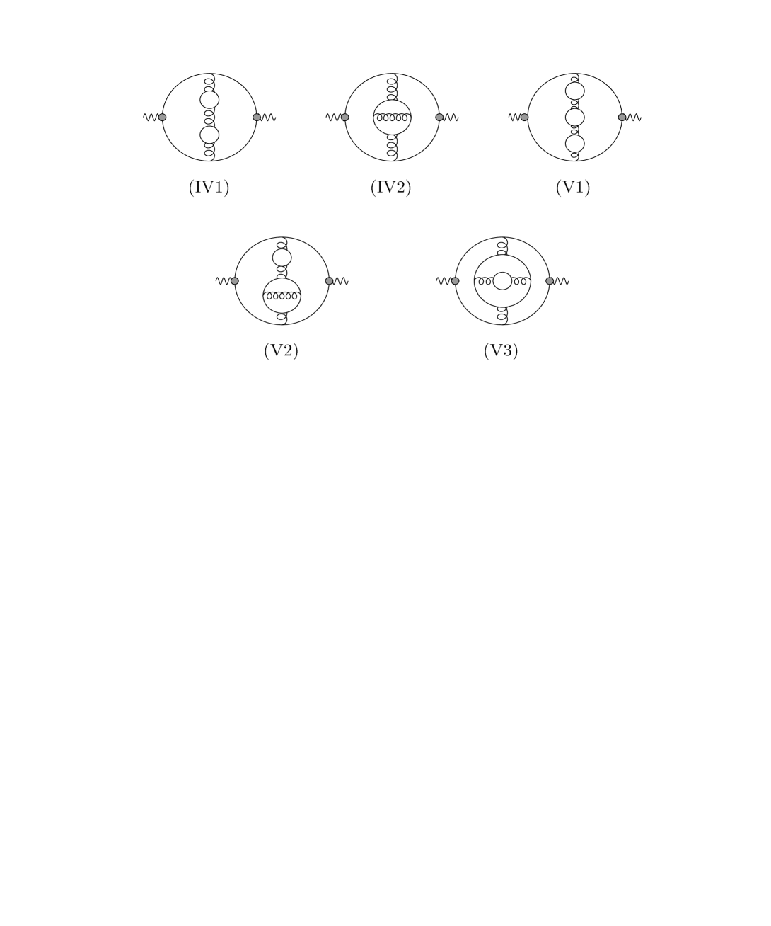
Figure 7: Representative abelian four- and five-loop diagrams for the hadronic vacuum polarization. It is understood that all self-energy type diagrams are added to each class of diagrams.

In this Appendix we collect the abelian five-loop diagrams to the hadronic vacuum polarization that are included in the scale-setting in next-to-leading order as described in Sect. 5. For completeness, we also list the four-loop diagrams. Numerical values are given for

$$Q^{2}\frac{d\Pi(Q^{2})}{dQ^{2}}=\frac{1}{4\pi^{2}}\sum_{n=0}^{\infty}D_{n+1}\left(\frac{\alpha(Q)}{\pi}\right)^{n}\,.$$ (C.1)

The diagrams are shown in Fig. 7. Each diagram shown stands for the class of diagrams obtained, when one adds the diagrams where gluons form self-energy type insertions rather than exchange type topologies. Diagram (V2) also includes the symmetric diagram, where the two inner loops are interchanged. We obtain:

$$D_{4}^{\mbox{\tiny(IV1)}} = C_{F}(TN_{f})^{2}\left[\frac{151}{54}-\frac{19}{9}\zeta(3)\right]$$ (C.2)

$$D_{4}^{\mbox{\tiny(IV2)}} = C_{F}(C_{F}TN_{f})\left[-\frac{101}{64}+\frac{3}{2}\zeta(3)\right]$$ (C.3)

$$D_{5}^{\mbox{\tiny(V1)}} = C_{F}(TN_{f})^{3}\left[-\frac{6131}{972}+\frac{203}{54}\zeta(3)+\frac{5}{3}\zeta(5)\right]$$ (C.4)

$$D_{5}^{\mbox{\tiny(V2)}} = C_{F}(TN_{f})(C_{f}TN_{f})\left[\frac{3571}{576}-\frac{59}{8}\zeta(3)+2\zeta(3)^{2}\right]$$ (C.5)

$$D_{5}^{\mbox{\tiny(V3)}} = C_{F}(TN_{f})(C_{f}TN_{f})\left[\frac{10199}{3456}-\frac{7}{2}\zeta(3)+\zeta(3)^{2}\right]$$ (C.6)

Here $T=1/2$, $C_{F}=4/3$ for $SU(3)$ with fermions in the fundamental representation and $T=1$, $C_{F}=1$ for $U(1)$. The sum of these terms yields $d_{2}^{\rm NLO}$ and $d_{3}^{\rm NLO}$ in QED (after proper normalization).

References

- [1] S. J. Brodsky, G. P. Lepage and P. B. Mackenzie, Phys. Rev. D28 (1983) 228
- [2] D. J. Broadhurst, Talk presented at the Workshop “Advances in non-perturbative and perturbative techniques”, Ringberg, Germany, November 1994
- [3] D. J. Broadhurst and A. G. Grozin, OUT–4102–52 [hep-ph/9410240]
- [4] M. Beneke and V. M. Braun, DESY-94-200 [hep-ph/9411229], to appear in Phys. Lett. B
- [5] G. P. Lepage and P. B. Mackenzie, Phys. Rev. D48 (1993) 2250
- [6] M. Neubert, CERN-TH-7487/94 [hep-ph/9412265]
- [7] S. J. Brodsky and H. J. Lu, SLAC-PUB-6481 [hep-ph/9405218]
- [8] G. Grunberg and A. L. Kataev, Phys. Lett. B279 (1992) 352
- [9] G. Sterman, Nucl. Phys. B281 (1987) 310
- [10] F. Le Diberder and A. Pich, Phys. Lett. B286 (1992) 147
- [11] V. I. Zakharov, Nucl. Phys. B385 (1992) 452
- [12] B. H. Smith and M. B. Voloshin, Phys. Lett. B340 (1994) 176
- [13] P. Ball, M. Beneke and V. M. Braun, in preparation
- [14] M. Beneke, Nucl.Phys. B405 (1993) 424
- [15] E. Speer, J. Math. Phys. 9 (1968) 1404; Generalized Feynman Amplitudes (Princeton Univ. Press, 1969)
- [16] D. J. Broadhurst, Z. Phys. C58 (1993) 339
- [17] M. Beneke and V. M. Braun, Nucl. Phys. B426 (1994) 301
- [18] M. Neubert and C.T. Sachrajda, CERN–TH-7312/94 [hep-ph/9407394]
- [19] M. Luke, A. Manohar and M.J. Savage, UTPT–94-21 [hep-ph/9407407]
- [20] M. Beneke, V. M. Braun and V. I. Zakharov, Phys. Rev. Lett. 73 (1994) 3058
- [21] E. Braaten, S. Narison and A.Pich, Nucl. Phys. B373 (1992) 581
- [22] Recent reviews are given by A. Pich, FTUV–94–71 ( 1994) [hep-ph/9412273] and S. Narison, CERN–TH-7506-94 [hep-ph/9412295]
- [23] S. G. Gorishny, A. L. Kataev and S. A. Larin, Phys. Lett. B259 (1991) 144; L. R. Surguladze and M. A. Samuel, Phys. Rev. Lett. 66 (1991) 560 [Erratum: ibid. 66 (1991) 2416]
- [24] G. Altarelli, in QCD – 20 years later, P. M. Zerwas and H. A. Kastrup (eds.), World Scientific (1993), Vol. 1, p. 172
- [25] C.A. Dominguez, UCT–TP-221-94 [hep-ph/9411331]
- [26] M. Beneke, PhD Thesis, Technische Universität München, 1993
- [27] G. Altarelli, P. Nason and G. Ridolfi, CERN-TH.7537/94 [hep-ph/9501240]
- [28] L. S. Brown and L. G. Yaffe, Phys. Rev. D45 (1992) 398; L. S. Brown, L. G. Yaffe and C. Zhai, Phys. Rev. D46 (1992) 4712
- [29] M. Beneke and V. I. Zakharov, Phys. Rev. Lett. 69 (1992) 2472
- [30] A. Duncan and S. Pernice, Univ. of Pittsburgh preprint, PITT-94-07
- [31] M. A. Shifman, A. I. Vainshtein and V. I. Zakharov, Nucl.Phys. B147 (1979) 385
- [32] V. P. Spiridonov and K. G. Chetyrkin, Sov. J. Nucl. Phys. 47 (1988) 522
- [33] G. ’t Hooft, in The Whys of Subnuclear Physics, Proc. Int. School, Erice, 1977, A. Zichichi (ed.) (Plenum, New York, 1978)
- [34] Ya. I. Azimov, Sov. J. Nucl. Phys. 11 (1970) 115
- [35] M. Beneke, Phys. Lett. B307 (1993) 154
- [36] M. Shifman, in Proc. of “Continuous Advances in QCD” (World Scientific, Singapure), Univ. of Minnesota preprint TPI-MINN-94/17-T [hep-ph/9405246]
- [37] I. Bigi et al., Phys. Rev. D50 (1994) 2234
- [38] N. Gray et al., Z. Phys. C48 (1990) 673
- [39] A. Palanques-Mestre and P. Pascual, Comm. Math. Phys. 95 (1984) 277
- [40] A. H. Mueller, Nucl. Phys. B250 (1985) 327
- [41] M. Beneke, Phys. Lett. B344 (1995) 341
- [42] M. Neubert, CERN preprint CERN-TH.7524/94 [hep-ph/9502264]