TPI–MINN–95–02/T NUC–MINN–95–8/T HEP–MINN–95–1327 hep-ph/9502289 February 1995 Gluon Production from Non-Abelian Weizsäcker-Williams Fields in Nucleus-Nucleus Collisions

Abstract

We consider the collisions of large nuclei using the theory of McLerran and Venugopalan. The two nuclei are ultra-relativistic and sources of non-abelian Weizsäcker-Williams fields. These sources are in the end averaged over all color orientations locally with a Gaussian weight. We show that there is a solution of the equations of motion for the two nucleus scattering problem where the fields are time and rapidity independent before the collision. After the collision the solution depends on proper time, but is independent of rapidity. We show how to extract the produced gluons from the classical evolution of the fields.

1 Introduction

Nucleus-nucleus collisions at ultra-relativistic energy have long been recognized as an environment where hot dense matter is formed [1, 2, 3]. It has been conjectured that in such an environment one might produce and experimentally study a quark-gluon plasma [4]. Theoretical studies of quark-gluon plasma formation have typically assumed some initial conditions at some time after the collision was initiated, and then evolved the matter distributions forwards in time according to the equations of perfect fluid hydrodynamics [3, 5].

While such an approach may work well for the late stages of the collision when the particles are not so energetic, it does not work well for the earliest stages of the collision. In the earliest stages, the quarks and gluons emerge from their quantum mechanical wavefunction and cannot be described as a perfect fluid until at least enough time has passed for there to be scattering.

In the earliest stages of the collision, the quark and gluon interactions should be most energetic. Such scatterings are therefore more easy to experimentally probe as they presumably induce hard experimental signatures which are more easily disentangled from backgrounds due to soft final state processes. During the hydrodynamic expansion, typically the scale of energy in the interaction is softer and more difficult to disentangle from backgrounds.

There has been recent progress in attempting to describe the early evolution of matter produced in nuclear collisions [6]. In the parton cascade model of Geiger and Müller, one takes the experimentally measured distribution functions for quarks and gluons and assumes that they may be treated as an incoherent beam of particles arising from each nucleus. The scattering of partons from partons is computed making reasonable assumptions about quantum coherence and time dilation effects. The system is thereby evolved from very early times in the collision until a later time when hydrodynamics may be applicable. In such a theory, the hard scattering signals are computed and may be compared with experiment.

The parton cascade model while elegant and well motivated, in our opinion still lacks some theoretical underpinning. In particular, the issue of quantum coherence in the initial state is treated phenomenologically, and needs a deeper understanding. This problem has at least two important aspects.

The first and most glaring problem is that the partons arise from a quantum mechanical state. In such a state the uncertainty in momentum, $\Delta p$, times the uncertainty in position, $\Delta x$, is close to saturated,

$$\Delta p\Delta x\sim 1$$ (1)

For example, in the longitudinal momentum distribution of partons, the wee partons have a longitudinal momentum of order of $100$’s of $MeV$. This corresponds to a longitudinal size of order of fractions of a Fermi. On the other hand, in the parton cascade one assumes knowledge of both the position and momentum of the partons, since the partons are described by classical phase space distribution functions. While this should be true later in the collision as the scale of spatial gradients becomes larger, early in the collision it is most certainly violated.

Although in the parton cascade, the assumptions on the initial distributions are plausible, they can at best give a qualitative agreement with precise results which include the effects of coherence, and at worst totally ignore some classes of interference phenomena. For example, one obvious problem is that for a single nucleus, the partons will spread out since they are an incoherent distribution of partons with different momentum. After some time, one therefore no longer has a spatially compact nucleus.

Another class of phenomena which is not fully treated in the parton cascade model is the problem of coherent addition of the color charges of quarks and gluons. Such coherent addition is for example responsible for Debye screening, and presumably magnetic screening, which will serve as a cutoff for divergent transport cross sections in parton-parton processes. In the parton cascade, a low momentum cutoff is introduced by hand, and of course results for many processes depend upon this cutoff.

While the parton cascade may lack precision in many detailed computations, it nevertheless is outstanding for its qualitative predictions. We nevertheless would like to put this model onto firmer foundations, and understand clearly its limits of applicability.

To begin to tackle this problem, one must understand at least some aspects of the quantum mechanical wavefunction of the quarks and gluons in the nuclear wavefunction. In the past, one rarely considered the nuclear wavefunction, and the structure functions for a nucleus were taken as a given quantity. There was no constructive description of how such structure functions arise.

Recent work by McLerran and Venugopalan has given rise to a picture of how the structure functions arise at small x for very large nuclei at ultra-relativistic energy. In this description, the effects of quantum and charge coherence of the partons in the nuclear wavefunction are properly included. The gluons arise from the non-abelian Weizsäcker-Williams fields generated by the color charges of the valence quarks.

In this paper, we will extend the treatment of McLerran and Venugopalan from a description of a single nucleus to the collision of two nuclei. This work is in some sense an extension of early effort which were somewhat ad hoc to describe such collisions by classical fields [8, 9]. We will see that in the region where most of the parton density sits, the gluon distribution function can initially be described by a classical field. These classical fields are to be interpreted as resulting from coherently superimposing large numbers of gluonic quanta. This way the classical description, wherever applicable will automatically incorporate coherence effects.

The gluon field for a single nucleus arising in this way is a non-abelian Weizsäcker-Williams field. At the initiation of the collision, the non-abelian Weizsäcker-Williams fields of the two nuclei play the role of boundary conditions for the time evolution of the gluon field. This classical field eventually evolves into gluon quanta.

The picture we have of the collision is therefore the following. Before the nuclei collide, they are described by valence quarks and their coherent Weizsäcker-Williams fields. These fields are classical in the sense of classical electromagnetic fields, but of course can not be thought of as composed of particle with classical phase space distributions. During the collision, the fields are still classical, but sufficiently strong so that the equations of motion evolve the fields non-linearly with time. As time evolves, the field weakens. When the strength of the gluon field is sufficiently low, the field equations linearize, and the gluon field describes the evolution of weakly interacting classical gluon waves. At this time, the coherent addition of the fields is no longer important, and they should be described by an incoherent distribution of gluons. The parton cascade model may therefore be used.

Prior to this time however, the coherence in the gluon field is essential. The simple fact that the evolution of the gluons is described by a classical field is a consequence of the fact that the gluons are in some locally coherent state. A description in terms of incoherent classical particles is simply not possible.

In the second section, we review the relevant results of computation of the small x structure functions for a single large nucleus. We will attempt to describe the kinematic limits of applicability of this description. We will argue that the Weizsäcker-Williams fields should describe the distribution of gluons in the region of transverse momenta which gives the dominant contribution after integrating over transverse momenta.

In the third section, we set up the problem of nucleus-nucleus scattering. We derive an equation for the time evolution of the gluon field. We relate the results of such a computation to the phase space density of gluon radiation.

In the fourth section, we summarize our results and speculate on their region of validity.

2 Review of the McLerran-Venugopalan Model

In the work of McLerran and Venugopalan [7], it was argued that for very large nuclei, $A^{1/3}\rightarrow\infty$ at small values of Bjorken $x$, $x<<A^{-1/3}$, the quark and gluon distribution functions are computable in a weak coupling limit. This is because the density of partons per unit area defines a dimensionful scale and when

$$\mu^{2}\sim{1\over{\pi R^{2}}}{{dN}\over{dy}}>>\Lambda_{QCD}^{2}$$ (2)

the strong coupling parameter $\alpha_{S}(\mu^{2})$ should become small. Here $y\sim\ln(1/x)$.

In lowest order in a naive weak coupling expansion, it was shown that the gluon distribution function was of the Weizsäcker-Williams form, that is proportional to $1/x$. It was also shown that the $p_{\perp}$ dependence was also of the Weizsäcker-Williams form $dN/d^{2}p_{\perp}\sim 1/p_{\perp}^{2}$ for $\alpha_{S}\mu<<p_{\perp}<<\mu$ where $\mu\sim\Lambda_{QCD}A^{1/6}$

Of course the naive weak coupling expansion may not be strictly valid, since there is the well known Lipatov enhancement of the low x structure functions [10]. This enhancement involves quantum corrections to the lowest order naive weak coupling result, and changes the small x distribution to $1/x^{1+C\alpha_{s}}$. While this behavior is computable in the McLerran-Venugopalan model, its nature is not yet fully understood. We expect however that as far as the local effects on the parton distribution at fixed rapidity, $y\sim\ln(1/x)$, the main effect is to renormalize the charge which generates the Weizsäcker-Williams field.

The charge which generates this field in lowest order in the naive weak coupling expansion is the charge of the valence quarks which are treated in a no recoil approximation. While it may be true that the Lipatov correction might involve new physics, and the picture might change, we will ignore its effects here except to state that we believe it will effectively renormalize the valence quark charge through some x dependent source of charge. To see how this might occur, recall that the strength of the Weizsäcker-Williams distribution is proportional to the amount of charge present at a value of x larger than that of the distribution. We are therefore assuming the main effect of the quantum fluctuations is to generate an excess amount of charge at values of x larger than that at which we measure the parton.

In the work which follow, we will not treat the problems generated by the Lipatov effect. We will instead concentrate on the naive lowest order approximation to the McLerran-Venugopalan model. This will be sufficient to understand many qualitative aspects of nucleus-nucleus collisions, and we hope in the end with small modifications can also be extended to include the effects of the Lipatov enhancement.

In Refs. [7], it was found that to compute the structure functions one simply treated the valence quarks as a source of light cone charge.

Here the valence quarks are being treated as a source of charge moving at the speed of light along the light cone $x^{-}=0$. The source of charge is being treated classically. This approximation as justified so long as the typical transverse momentum scale is

$$p_{\perp}<<\mu$$ (3)

where $\mu$ is proportional to the number of valence quarks per unit area.

At the same time the number of gluon quanta at resolutions with $p_{\perp}<<\mu$ will be sufficiently high to allow for a description of the gluonic degrees of freedom through a classical field.

Within these limits, all one has to do is to formulate and solve the Yang-Mills equations in the presence of the classical current induced by the valence quarks:

$$\left[D_{\mu},F^{\mu\nu}\right] = U[A](x,z(x))\,J^{\nu}(z(x))\,U[A](z(x),x)\qquad.$$ (4)

Here $z(x)=\left.x\right|_{x^{+}=0}$ serves as a reference point used to define “initial values” for the color distribution of the valence quarks

$$J^{\nu}(z(x))=\delta^{\nu+}\delta(x^{-})\rho(x_{\perp})$$ (5)

which then, due to covariant current conservation $\left[D_{\nu},J^{\nu}(x)\right]=0$ evolve along the particles trajectory via parallel transport or link operators $U[A](x,z(x)):={\rm P}\exp-ig\int_{z(x)}^{x}\!\!d{x^{\prime}}^{+}A^{-}({x^{\prime}}^{+},x_{\perp},x^{-}=0)$ connecting the points $x$ and $z(x)$ along the particles trajectory.

Given a solution to the equations of motion, charge density $\rho$ is to be treated as a stochastic variable, and to compute ground state expectation values one must average over all sources with a local Gaussian weight

$$\int[d\rho]\ \exp\left\{-\int d^{2}x_{\perp}{1\over{2\mu^{2}}}\rho(x_{\perp})^{2}\right\}$$ (6)

This Gaussian distribution arose from the approximations used in Ref. [7]. It was argued there that on the transverse resolution scales corresponding to $p_{T}<<\mu$ that the valence quark charges may be treated classically. The exponential factor is the contribution to the phase space density associated with counting the number of states of valence charges for a fixed value of the classical charge. It can be thought of as arising from the following classical picture. Suppose we look in a tube through the nucleus. This tube has a transverse size much less than a Fermi but large enough so that it intersects many nucleons. In this case, there will typically be many valence quarks inside the tube each coming from a different nucleon. The color charge of each quark is therefore uncorrelated with that of any other quark and the color charges will add together in a random walk. This will lead to the above Gaussian distribution.

Physically, the picture one has is the following: The valence quarks are recoilless sources of color charge propagating along the light cone. Their charge can fluctuate from process to process and the averaging over charges corresponds to this fluctuation. The local charge density is therefore a random variable. The reason why such a stochastic source of charge arises is because the transverse resolution scales which we are interested in are small compared to a fermi. On such a scale, when one looks at the nucleus, one sees uncorrelated quarks coming from different nucleons. The source of color charge therefore random walks in color space. The criteria that $p_{\perp}<<\mu$ is the criteria that within each transverse resolution scale, there are many quarks so that the color charge is typically large and can be treated classically.

The solutions of the above Yang-Mills equations can be chosen to be of the form

$$A^{+} = 0$$

$$A^{-} = 0$$

$$A^{i} = \theta(x^{-})\alpha_{i}(x_{\perp})$$ (7)

Here the first line may be interpreted gauge choice. Using light cone gauge $A^{+}=0$ one has direct access to the gluon distribution functions of the parton model. The requirement to have $A^{-}=0$ then could still be implemented as a gauge choice at least along the trajectories of the particles, making use of the residual gauge freedom present in any axial gauge. In this case it turns out that there is a particular solution to the equations of motion which has $A^{-}$ vanishing everywhere. On such a solution the link operators on the right hand side of the Yang-Mills equations drop out entirely and the equations become

$$F^{ij} = 0$$

$$\nabla\cdot\alpha = \rho(x_{\perp})$$ (8)

The solution to these equations is that

$$\alpha_{i}=-{1\over{ig}}U(x_{\perp})\nabla_{i}U^{\dagger}(x_{\perp})$$ (9)

that is a pure two dimensional gauge transform of a the vacuum.

Physically, this solution is also easy to understand. The solution is a gauge transform of vacuum on one side of the sheet of valence charge, and another gauge transform of vacuum on the other side of the sheet. We have chosen the field to be zero on one side of the sheet as an overall gauge choice. (This could be relaxed by an overall gauge transformation). Because of the discontinuity in the fields at the sheet of valence charge, the solution is not a gauge transform of the vacuum fields. Its discontinuity gives the source of valence charge.

Although we have not been successful in explicitly finding the solution to this equation, it is in principle possible to do numerically. Several generic features of the averaging over different sources of charge are possible to infer nevertheless.

For $p_{\perp}\leq\alpha_{S}\mu$, the typical value of the external charge is so large that it is a bad approximation to linearize the gauge transformation and directly compute the field in a naive weak coupling expansion. In this region, the non-linearities of the field equation become important.

In this kinematic region, the shape of the Weizsäcker-Williams distribution changes form, as is shown in Fig. 1.

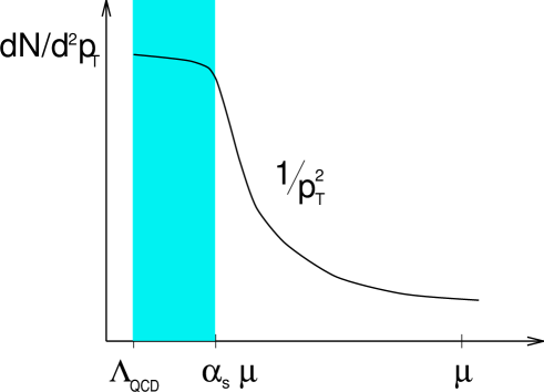
Fig. 1: Weizsäcker-Williams distribution for a single nucleus

The $1/p^{2}_{\perp}$ behavior turns over and goes to a constant. This provides a low momentum cutoff in the number of gluons generated by the distribution. At high momentum, we can compute no further than $p_{\perp}\leq\mu$. The distribution should nevertheless extend beyond this region. In fact the upper momentum cutoff should be determined only by the kinematic limit of the process considered. Strictly speaking the number of Weizsäcker-Williams gluons is infinite, but only logarithmically, and the cutoff will be determined by the process of physical interest.

Suppose we consider the production of gluons in a two nucleus collision. We can naively determine the cutoff in momentum of produced gluons. Lets us assume that we are in the weak coupled perturbative region. The rate must be proportional to the density squared of gluons, so that it must be proportional to $\alpha_{S}^{2}\mu^{4}$. It involves scattering, so their are two more factors of $\alpha_{S}$. Therefore on dimensional grounds, we expect that the probability of making a pair of on mass shell gluons should be of order $\alpha_{S}^{4}\mu^{4}/p_{\perp}^{4}$. This is of order one when $p_{\perp}\sim\alpha\mu$, that is at precisely the place where the fields evolve non-linearly. It cuts off rapidly in $p_{\perp}$, so that the number of produced gluons should be ultraviolet finite.

This example teaches us two things: First that for a physical process there is no ultraviolet divergence and for this process the important contribution for gluon production is at scales less than $\mu$. Second, that the process is strongest in the region where the field is strong. In this region, the field is evolving non-linearly, and the coherence of the field is important. It would therefore be a mistake to assume that the distribution of produced gluons reflects the distribution in the initial nuclei. This is true for gluons with $p_{\perp}\geq\alpha_{S}\mu$, that is ’hard gluons’, but the softer gluons which dominate the production are in a non-linear region.

The appearance of these non-linearities might be qualitatively included in the parton cascade model. However insofar as there is an infrared cutoff dependence in some physical process, the results will be somewhat quantitatively unreliable. Processes without such a cutoff dependence would of course be more reliably computed.

The hope will be in our attempt to compute gluon production is that the classical non-linearities will cutoff the the naive divergence in the production amplitude at small $p_{\perp}$. To see that this is plausible, recall that the single gluon distribution changes its from at small $p_{\perp}$ from $1/p_{\perp}^{2}$ to constant at $p_{\perp}\leq\alpha_{S}\mu$. It is therefore quite plausible that these effects in fact cutoff the singularity at some scale of order $\alpha_{S}\mu$. If this is so, then if $A$ is large enough so that $A^{1/6}>>1$, this cutoff is at a scale much larger than $\Lambda_{QCD}$, and the computation is self-consistent.

3 The Two Nucleus Problem

We now turn to the problem of nucleus-nucleus scattering. We work in the center of mass frame. Both nuclei are at sufficiently high energy so that they can be treated as infinitesimally thin sheets. They are large enough so that these sheets can be taken to be of infinite extent in the transverse direction. We will be interested in describing the production of gluons at typical momentum scales which are $p_{\perp}<<\mu$, but much larger than $200~{}MeV$. In this case the source of color charge can be taken as classical as in the McLerran-Venugopalan model. The charge is of course a stochastic variable which must be integrated over with a Gaussian weight as described in the previous section.

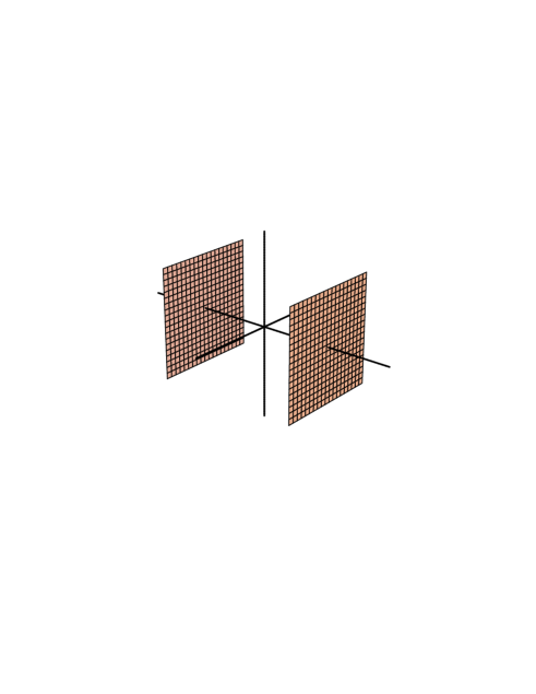
Fig. 2: Two nuclei Lorentz-contracted to infinitely thin sheets before the collision takes place

The sources of color field set up a classical color field. After the collision the color field will begin to evolve in time. Much after the collision, the color field will describe the propagation of free gluons. In this section we will describe how to compute the evolution of the color field, and then how to compute the final state distribution of gluons.

The Yang-Mills equation for the two source problem is

$$\left[D_{\mu},F^{\mu\nu}\right]=J^{\nu}(x)$$ (10)

where

$$J^{+} = \delta(x^{-})\rho_{1}(x_{\perp})$$

$$J^{-} = \delta(x^{+})\rho_{2}(x_{\perp})$$

$$J^{i} = 0$$ (11)

and we have restricted ourselves to work in a gauge where the link operators along the particle trajectories drop out.

Before the collision takes place, we find a solution of the equations of motion to be

$$A^{+} = 0$$

$$A^{-} = 0$$

$$A^{i} = \theta(x^{-})\theta(-x^{+})\alpha^{i}_{1}(x_{\perp})+\theta(x^{+})\theta(-x^{-})\alpha^{i}_{2}(x_{\perp})$$ (12)

This is a solution of the Yang-Mills equations in all of space-time except on or within the forward light cone, as shown in Fig. 3.

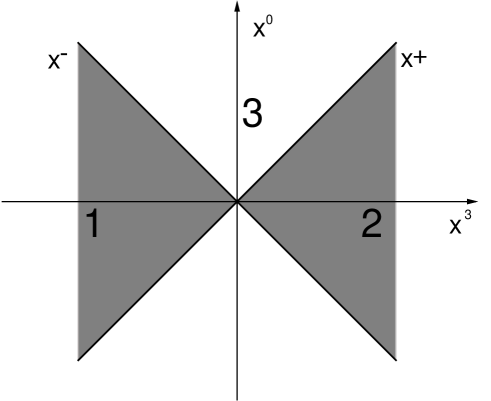
Fig. 3: Regions with different structures of the gauge potential:
In regions 1 and 2 we have the well known one nucleus solutions $\alpha_{1,2}$. While in the backward light cone there the gauge potential is vanishing we have a nontrivial solution in the forward lightcone, region 3

In the forward light cone, we must add in extra pieces in order to have a solution. This will be done below. The two dimensional vector potentials are pure gauges and solve for $t<0$

$$\nabla\cdot\alpha_{1,2}=\rho_{1,2}(x_{\perp})$$ (13)

The physical picture one has of this solution prior to the collision is that the nuclei have zero field in front of them as they approach one another. Behind them the field is pure gauge. Because each nucleus has a different charge density, the gauge is different for each nucleus. This is an exact solution of the equations of motion so long as one is outside the forward light cone, that is in regions which are out of causal contact from the collision event.

The fact that we have a solution of the equations of motion which does not evolve in time before the collision is remarkable. This solves the problem of cascade models that an isolated nucleus composed of partons will spontaneously fall apart. Here the individual nuclei and their parton clouds are static except for their overall center of mass motion.

How do we describe the fields after the collision? Except at the forward light cone, that is, when we are inside or outside the cone, the fields satisfy free field equations. We will look for a Lorentz covariant solution to the equations of motion. We try, for $x^{-}>0$ and $x^{+}>0$

$$A^{+} = x^{+}\alpha(\tau,x_{\perp})$$

$$A^{-} = x^{-}\beta(\tau,x_{\perp})$$

$$A^{i} = \alpha_{3}^{i}(\tau,x_{\perp})$$ (14)

where

$$\tau=\sqrt{t^{2}-z^{2}}=\sqrt{2x^{+}x^{-}}$$ (15)

This solution only depends on the longitudinal boost invariant variable $\tau$ and has no dependence on the space-time rapidity variable

$$\eta={1\over 2}\ln{x^{+}\over x^{-}}$$ (16)

The factors of $x^{+}$ and $x^{-}$ in the definition of the vector potential guarantee that under longitudinal boosts, the vector potential transforms properly.

By making a gauge transformation which is only a function of proper time and $x_{\perp}$,

$$U=U(\tau,x_{\perp})$$ (17)

we see that we can fix

$$\beta(\tau,x_{\perp})=-\alpha(\tau,x_{\perp})$$ (18)

which we shall choose to do. This choice corresponds to a gauge condition

$$x^{+}A^{-}+x^{-}A^{+} = 0$$ (19)

which in turn is consistent with dropping the link-operators in (10).

If such a solution solves the equations of motion an boundary conditions, it will predict that the distribution of partons is boost invariant. It is the generalization therefore of Bjorken’s boost invariant hydrodynamic equations to the equations which generate the initial conditions for the hydrodynamic equations.

As a consequence of the boost invariance of the Yang-Mills equations, the ansatz above solves the equations within the forward light cone. This can be checked explicitly. The equations which result for $\alpha_{3}^{i}$, and $\alpha$, for $x^{+},x^{-}>0$ are

$${1\over\tau^{3}}\partial_{\tau}\tau^{3}\partial_{\tau}\alpha-\left[D^{i},\left[D^{i},\alpha\right]\right] = 0$$

$${1\over\tau}\left[D_{i},\partial_{\tau}\alpha_{3}^{i}\right]+ig\tau\left[\alpha,\partial_{\tau}\alpha\right] = 0$$

$${1\over\tau}\partial_{\tau}\tau\partial_{\tau}\alpha^{i}_{3}-ig\tau^{2}\left[\alpha,\left[D^{i},\alpha\right]\right]-\left[D^{j},F^{ji}\right] = 0$$ (20)

These four equations can be checked to be consistent with on another. From this point on, all vector indices will refer to two dimensional transverse vectors. The longitudinal and time coordinates will be denoted separately.

In intermediate step in deriving the above equations, we computed the field strengths $F^{\mu\nu}$. The results of that computations are

$$F^{+-} = -{1\over\tau}\partial_{\tau}\tau^{2}\alpha$$

$$F^{ij} = \partial^{i}\alpha_{3}^{j}-\partial^{j}\alpha_{3}^{i}-ig\left[\alpha^{i}_{3},\alpha^{j}_{3}\right]$$

$$F^{i\pm} = -x^{\pm}\left({1\over\tau}\partial_{\tau}\alpha^{i}_{3}\mp\left[D^{i},\alpha\right]\right)$$ (21)

The only task which remains is to show that the above solution also satisfies the boundary conditions generated by the sources. For either $x^{-}<0$ or $x^{+}<0$, the ansatz above satisfies the equations trivially. We look first at the equation $\left[D_{\mu},F^{\mu i}\right]=0$. This has a delta function singularity at $x^{-}=x^{+}=0$ which requires that

$$\left.\alpha_{3}^{i}(0,x_{\perp})\right|_{\tau=0}=\alpha_{1}^{i}(x_{\perp})+\alpha_{2}^{i}(x_{\perp})$$ (22)

and there are no further discontinuities in this equation.

Now for $\left[D_{\mu},F^{\mu\pm}\right]=J^{\pm}$, we find that

$$\left.\alpha^{\vphantom{i}}(\tau,x_{\perp})\right|_{\tau=0}=-{ig\over 2}\left[{\alpha_{1}}_{i}(x_{\perp}),\alpha^{i}_{2}(x_{\perp})\right]$$ (23)

These two equations for $J^{\pm}$ reduce to the same boundary condition, and therefore neither $\alpha$ nor $\alpha_{3}^{i}$ are overconstrained, demonstrating once more that our ansatz contains the correct degrees of freedom.

Note that assuming the boundary conditions above, we are implicitly requiring that the solution be regular at $\tau=0$. It is easy to check that the quantities $\alpha$ and $\alpha^{i}_{3}$ can either be regular at the origin or diverge like $\alpha\sim 1/\tau^{2}$ and $\alpha^{i}\sim\ln(\tau)$. These singular solutions will lead to a divergent energy density, and are therefore not allowed.

So with the above two boundary conditions, the solution to the equations of motion are uniquely specified. This solution is remarkable since in spite of the possible asymmetry in the charge on either nuclei, the solution is up to trivial factors rapidity independent. This has amusing phenomenological consequences for the collisions of asymmetric nuclei. The distribution should be flat in rapidity. The height of the central plateau of course depends on the asymmetry in a non-trivial way.

In order to determine the gluon radiation produced by these fields, we must solve them at proper times long after the collision. We expect that the energy density will dissipate and therefore the field strengths will become small. Using the expressions above, we conclude that asymptotically, for large $\tau$,

$$\alpha(\tau,x_{\perp}) \rightarrow V(x_{\perp})\epsilon(\tau,x_{\perp})V^{\dagger}(x_{\perp})$$

$$\alpha^{i}_{3}(\tau,x_{\perp}) \rightarrow V(x_{\perp})\left[\epsilon^{i}(\tau,x_{\perp})-{1\over{ig}}\partial^{i}\right]V^{\dagger}(x_{\perp})$$ (24)

The solution should tend to a small field plus a gauge transformation. The value of this gauge transformation is determined by the field equations and has a non-trivial dependence on the sources. It results from solving the non-linear time evolution equations for the fields.

The equations of motion for the fields in the asymptotic region are linear for $\epsilon$ and $\epsilon^{i}$. The equations are

$${1\over\tau^{3}}\partial_{\tau}\tau^{3}\partial_{\tau}\epsilon-\nabla^{2}\epsilon = 0$$

$${1\over\tau}\partial_{\tau}\tau\partial_{\tau}\epsilon^{i}-\left(\nabla^{2}\delta^{ij}-\nabla^{i}\nabla^{j}\right)\epsilon^{j} = 0$$ (25)

Observe, that $\nabla^{i}\epsilon^{i}$ does not enter the asymptotic equations, so that there are in fact only two dynamical degrees of freedom in the solution, as must be the case.

The solutions to the above equations at asymptotically large $\tau$ are of the form

$$\alpha^{a}(\tau,x_{\perp}) = \int{{d^{2}k_{\perp}}\over{(2\pi)^{2}}}{1\over\sqrt{2\omega}}\left\{a_{1}^{a}(\vec{k}_{\perp}){1\over\tau^{3/2}}e^{ik_{\perp}\cdot x_{\perp}-i\omega\tau}+C.C.\right\}$$

$$\vec{\alpha}^{a,i}(\tau,x_{\perp}) = \int{{d^{2}k_{\perp}}\over{(2\pi)^{2}}}\kappa^{i}{1\over\sqrt{2\omega}}\left\{a_{2}^{a}(k_{\perp}){1\over\tau^{1/2}}e^{ik_{\perp}x_{\perp}-i\omega\tau}+C.C.\right\}$$ (26)

In this equation, the frequency $\omega=\mid k_{\perp}\mid$, and the vector

$$\kappa^{i}=\epsilon^{ij}k^{j}/\omega$$ (27)

The notation $+C.C.$ means to add in the complex conjugate piece.

To derive an expression for the energy density, we recall that $\tau$ is large. Near $z=0$, this implies that the range of $z$ where $\tau\sim t>>z$ that the solutions are $z$ independent. This means they asymptotically have zero $p_{z}$. Now suppose we are at any value of $z$, and $\tau$ is large but $t\sim z$. We can do a longitudinal boost to $z=0$ without changing the solution. Again in this frame the solution has zero $p_{z}$. We see therefore that for the asymptotic solutions that the space time rapidity is one to one correlated with the momentum space rapidity, that is at asymptotic times we find that

$$\eta={1\over 2}\ln(x^{+}/x^{-})=y={1\over 2}\ln(p^{+}/p^{-})$$ (28)

To proceed further, we compute the energy density in the neighborhood of $z=0$. Here asymptotically $\tau=t$. The energy in a box of size $R$ in the transverse direction and $dz$ in the longitudinal direction, with $L<<t$ becomes [13]

$$dE={{dz}\over t}\int{{d^{2}k_{\perp}}\over{(2\pi)^{2}}}\omega\sum_{i,b}\mid a_{i}^{b}(k_{\perp})\mid^{2}$$ (29)

Recalling that $dy=dz/t$, we find that

$${{dE}\over{dyd^{2}k_{\perp}}}={1\over{(2\pi)^{3}}}\omega\sum_{i,b}\mid a_{i}^{b}(k_{\perp})\mid^{2}$$ (30)

and the multiplicity distribution of gluons is

$${{dN}\over{dyd^{2}k_{\perp}}}={1\over\omega}{{dE}\over{dyd^{2}k_{\perp}}}$$ (31)

As we expect for a boost covariant solution, the multiplicity distribution is rapidity invariant.

Finally, we must comment a bit on the characteristic time scale for the dissipation of the non-linearities in the equations for the time dependent Weizsäcker-Williams fields. This is difficult to estimate in general, but scaling arguments should suffice to estimate the time scale. The basic point is that the typical momentum scale in the problem relevant for the formation of most of the gluons is $p_{\perp}\sim\alpha\mu$ which up to logarithms is $p_{\perp}\sim 200MeVA^{1/6}$. The characteristic time scale for the dissipation of the classical non-linearities should therefore be of order $\tau\sim 1/p_{\perp}$. This is in agreement with other estimate of the characteristic formation time for partons, and is in agreement with the model of Geiger and Müller.

4 Summary and Conclusions

We have derived a theory of the formation of gluons which is applicable for small x gluons in the collisions of very large nuclei. We have found that the gluon distributions as measured in deep inelastic scattering undergo an entirely non-trivial evolution in forming gluons which would be the initial conditions for a parton cascade. We have shown how one can compute these initial conditions.

After finding the initial conditions, the subsequent evolution might be described by a combination of the parton cascade and hydrodynamics.

There are many further problems to be addressed in this theory. The equations described above must be numerically solved. This will provide for initial conditions for average head on collisions. In addition it will predict the spectrum of fluctuations from collisions to collision. Perhaps the most interesting problem is to compute the hard particles produced during the early evolution of the distributions so as to find a precise quantitative test of the theory.

References

- [1] J. D. Bjorken, Lecture Series given at International Summer Institute for Theoretical Physics, Current Induced Reactions, Published in Hamburg Theor. Inst. 1975:93 (QCD:I83:1975)
- [2] R. Anishetty, P. Koehler and L. McLerran, Phys. Rev. D22, 2793 (1980).
- [3] J. D. Bjorken, Phys. Rev. D27, 140 (1983).
- [4] For a recent review see Quark Matter ’93, Proceedings of the Tenth International Conference on Ultra-relativistic Nucleus-Nucleus Collisions, Borlange, Sweden, June 20-24 (1993), edited by E. Stenlund, H-A Gustafsson, A. Oskarrson and I. Otterlund, North Holland Publishers.
- [5] G. Baym, B. L. Friman, J. P. Blaizot and M. Soyeur, Nucl. Phys. A407, 541 (1983).
- [6] K. Geiger and B. Müller, Nucl. Phys. B369, 600 (1992); K. Geiger, Phys. Rev. D47, 133 (1993); K. Geiger, Cern Preprint CERN-TH. 7313/94.
- [7] L. McLerran, R. Venugopalan, Phys. Rev. D49 2233 (1994); Phys. Rev. D49 3352 (1994).
- [8] H. Ehtamo, J. Linfors and L. McLerran, Z. Phys. C18, 341 (1983).
- [9] T. S. Biro, H. B. Nielsen and J. Knoll, Nucl. Phys. B245 (1984)
- [10] E. A. Kuraev, L. N. Lipatov and Y. S. Fadin, Zh. Eksp. Teor. Fiz 72, 3 (1977) ( Sov. Phys. JETP 45, 1 (1977)).
- [11] A. H. Mueller, Nucl. Phys. B415 373 (1994).
- [12] L. McLerran, R. Venugopalan, Phys. Rev. D50 2225 (1994).
- [13] J. P. Blaizot and A. Mueller, Nucl. Phys. B289, 847 (1987).